Presented By Dr. Shazzad Hosain Asst. Prof. EECS, NSU Phylogeny

Presented ByDr. Shazzad Hosain

Asst. Prof. EECS, NSU

Phylogeny

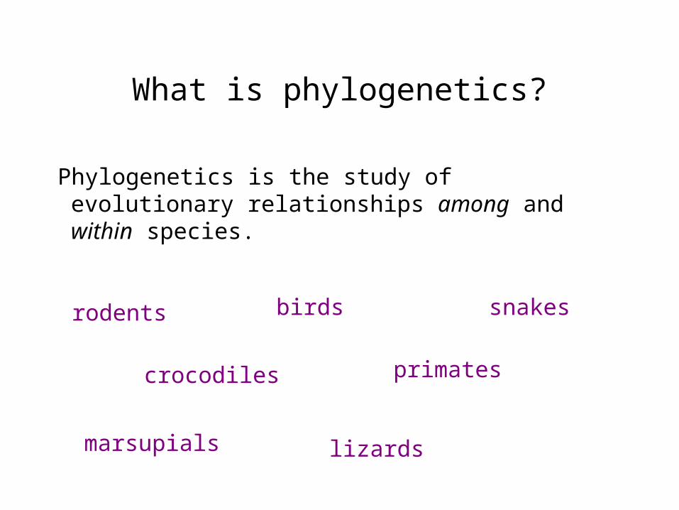
What is phylogenetics?

Phylogenetics is the study of evolutionary relationships among and within species.

crocodiles

birds

lizards

snakesrodents

primates

marsupials

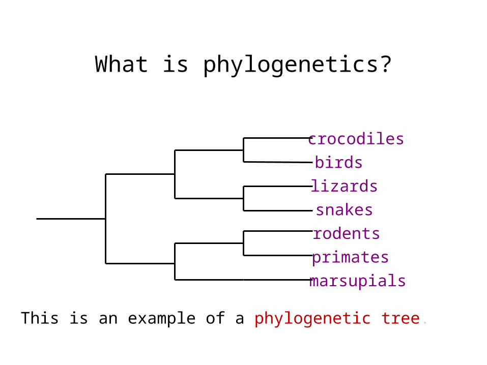
What is phylogenetics?

crocodilesbirdslizardssnakesrodentsprimatesmarsupials

This is an example of a phylogenetic tree.

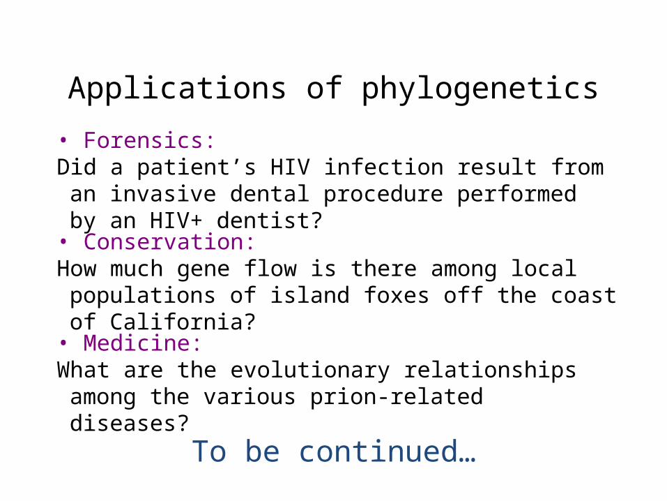
• Forensics:Did a patient’s HIV infection result from an invasive dental

procedure performed by an HIV+ dentist?

Applications of phylogenetics

• Conservation:How much gene flow is there among local populations of island

foxes off the coast of California?

• Medicine:What are the evolutionary relationships among the various

prion-related diseases?

To be continued…

Phylogenetic concepts:Interpreting a Phylogeny

Sequence A

Sequence BSequence C

Sequence D

Sequence E

Time

Which sequence is most closely related to B?

A, because B diverged from A more recently than from any other sequence.

Physical position in tree is not meaningful! Only tree structure matters.

Phylogenetic concepts:Rooted and Unrooted Trees

Time

A

B

C

D

Root =

A B

C D

Root

X

=?

A B

C D

?

? ?

? ?

X

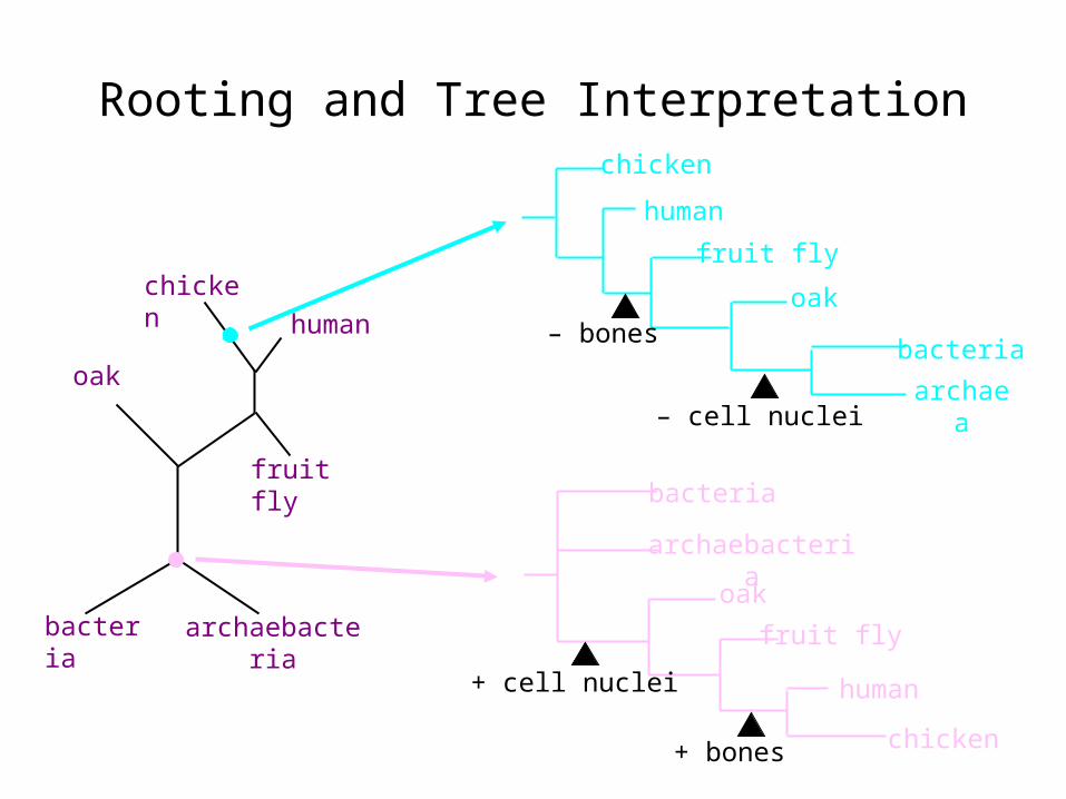
Rooting and Tree Interpretation

bacteria archaebacteria

oak

fruit fly

chickenhuman

bacteria

archaea

oak

fruit fly

chicken

human

bacteria

archaebacteria

oak

fruit fly

chicken

human

– bones

– cell nuclei

+ cell nuclei

+ bones

Rooting Methods

Given an unrooted network of relationships among four species of Carnivora [left], outgroup rooting uses an additional taxon (the outgroup) known from independent evidence to be less closely related to any of the other species (the ingroup) than they are to each other. The root is then placed on the branch between the outgroup and the ingroup. In this case, Lynx is a feloid carnivore in a separate superfamily from the four canoid carnivores. Inclusion of Lynx in the network analysis places it on the internode.This method requires accurate information as to ingroup / outgroup relationships.

Outgroup Rooting a network of relationships

How Many Trees?

Unrooted trees Rooted trees

# sequences

# pairwise distances # trees

# branches

/tree # trees# branches

/tree

3

4

5

6

10

30

N

(assuming bifurcation only)

How Many Trees?

2N - 2(2N - 3)!2N - 2 (N - 2)!

2N - 3(2N - 5)!2N - 3 (N - 3)!

N (N - 1)2

N

584.95 1038578.69 103643530

1834,459,425172,027,0254510

109459105156

8105715105

6155364

433133

# branches/tree# trees

# branches

/tree# trees# pairwise distances

# sequences

Rooted treesUnrooted trees

Tree Properties

Root

UltrametricityAll tips are an equal

distance from the root.X

Y

a

bc d

e

a = b + c + d + e

Root

AdditivityDistance between any two tips equals the total branch

length between them.

X

Ya

b

c de

XY = a + b + c + d + e

In simple scenarios, evolutionary trees are ultrametric and phylograms are additive.

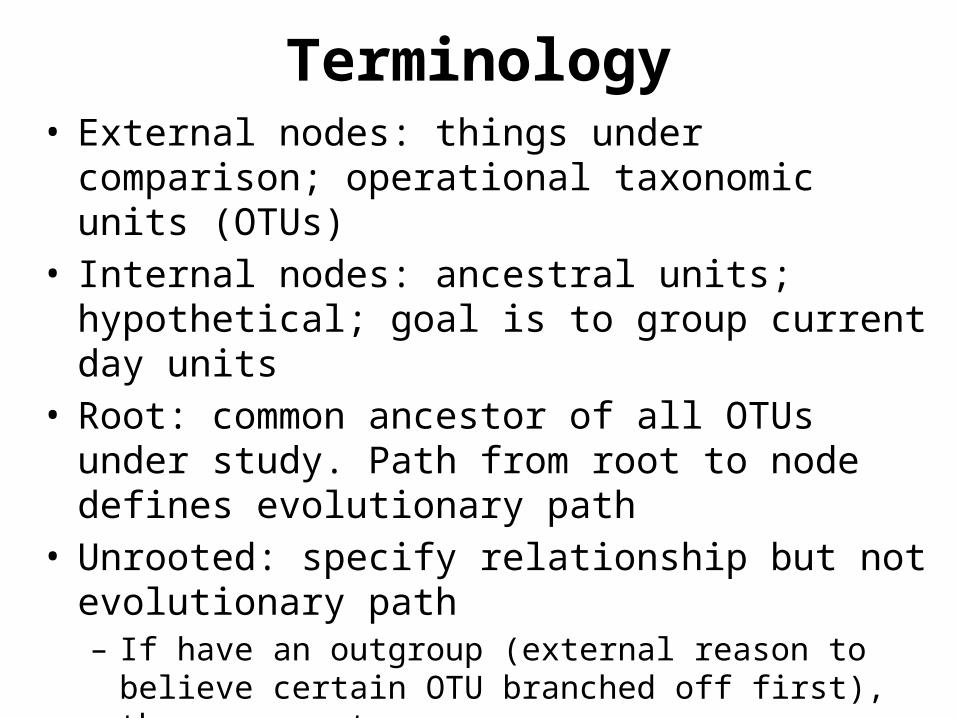
Terminology• External nodes: things under comparison; operational

taxonomic units (OTUs)• Internal nodes: ancestral units; hypothetical; goal is to

group current day units• Root: common ancestor of all OTUs under study. Path

from root to node defines evolutionary path• Unrooted: specify relationship but not evolutionary path

– If have an outgroup (external reason to believe certain OTU branched off first), then can root

• Topology: branching pattern of a tree• Branch length: amount of difference that occurred along

a branch

Phylogeny Applications

• Tree of Life: Analyzing changes that have occurred in evolution of different organisms http://tolweb.org/tree/phylogeny.html

• Phylogenetic relationships among genes can help predict which ones might have similar functions (e.g., ortholog detection)

• Follow changes occurring in rapidly changing species (e.g., HIV virus)

http://tolweb.org/tree/phylogeny.html

Phylogeny Packages

• PHYLIP, Phylogenetic inference package– evolution.genetics.washington.edu/phylip.html– Felsenstein– Free!

• PAUP, phylogenetic analysis using parsimony– paup.csit.fsu.edu– Swofford

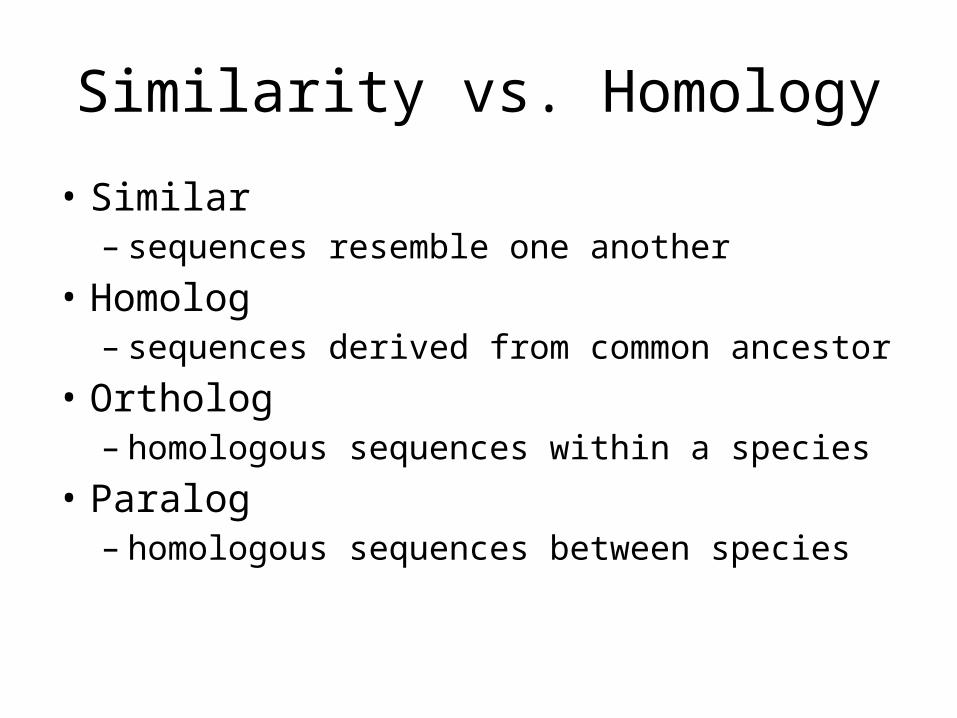
Similarity vs. Homology

• Similar– sequences resemble one another

• Homolog– sequences derived from common ancestor

• Ortholog– homologous sequences within a species

• Paralog– homologous sequences between species

Ortholog vs. Paralog

• Ortholog – genomic variation occurs after speciation – hence can be used for phylogeny of organism

• Paralog – genetic duplication occurs before speciation – hence not suitable for phylogeny of organism

Homoplasy

• Sequence similarity NOT due to common ancestry

• May arise due to parallelism or convergent evolution

• Parallelism or parallel evolution– the development of a similar trait in related, but

distinct, species descending from the same ancestor, but from different clades

• Convergent evolution

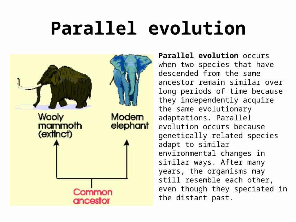
Parallel evolutionParallel evolution occurs when two species that have descended from the same ancestor remain similar over long periods of time because they independently acquire the same evolutionary adaptations. Parallel evolution occurs because genetically related species adapt to similar environmental changes in similar ways. After many years, the organisms may still resemble each other, even though they speciated in the distant past.

Convergent evolutionwhen species from different ancestors colonize the same environment, they may independently acquire the same adaptations. The evolution of species descended from different ancestors to become superficially similar because they are adapting to the same environment is called convergent evolution

Divergent Evolution

Phylogeny of what?

• Organisms– Whole genome phylogeny– Ribosomal RNA (surrogate for whole genome)

• Strains (closely related microbes)• Individual genes (or gene families)• Repetitive DNA sequences• Metabolic pathways• Secondary Structures• Any discrete character(s)• Human languages• Microbial communities

Why compute phylogenetic trees?

• Understand evolutionary history• Map pathogen strain diversity for vaccines• Assist in epidemiology

– Of infectious diseases– Of genetic defects

• Aid in prediction of function of novel genes• Biodiversity studies• Understanding microbial ecologies

Tree Building Exercises

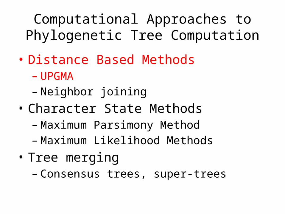
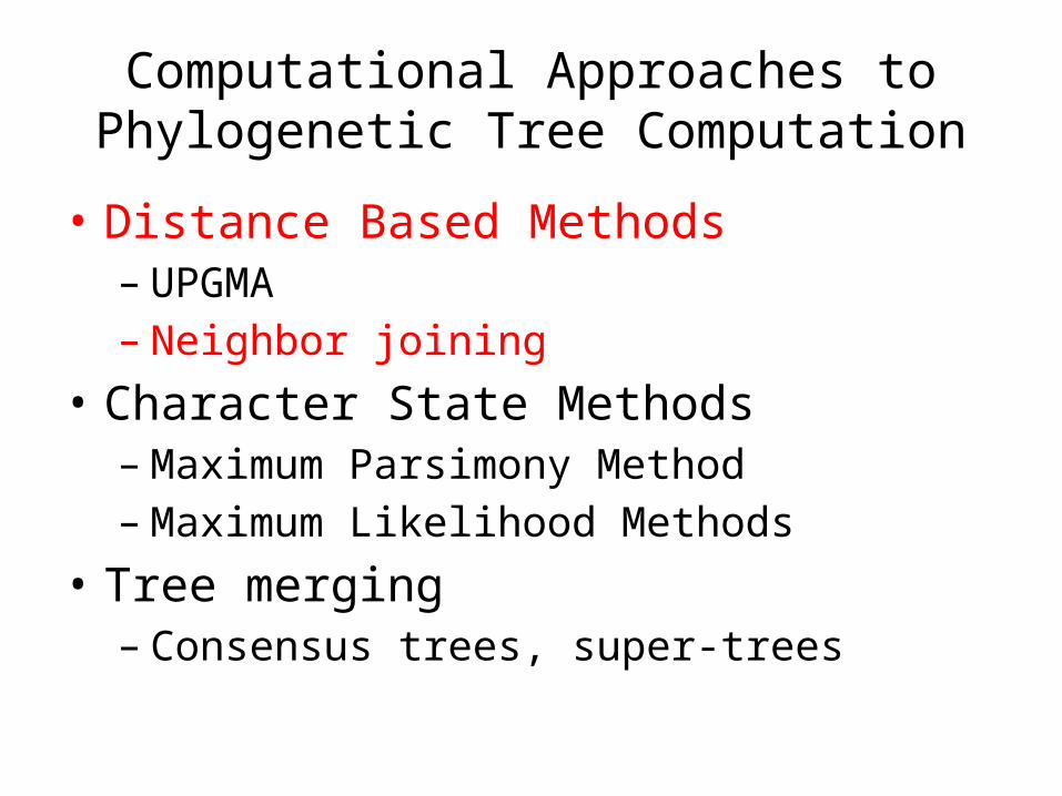
Computational Approaches toPhylogenetic Tree Computation

• Distance Based Methods– UPGMA– Neighbor joining

• Character State Methods– Maximum Parsimony Method– Maximum Likelihood Methods

• Tree merging– Consensus trees, super-trees

What data is used to build trees?

• Traditionally: morphological features (e.g., number of legs, beak shape, etc.)

• Today: Mostly molecular data (e.g., DNA and protein sequences)

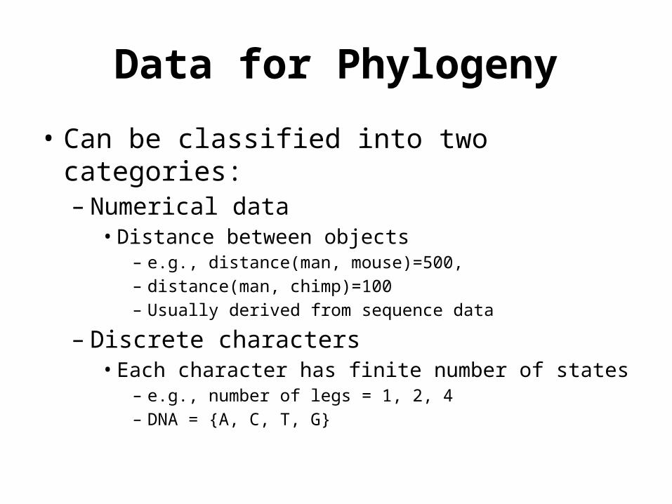
Data for Phylogeny

• Can be classified into two categories:– Numerical data

• Distance between objects– e.g., distance(man, mouse)=500,– distance(man, chimp)=100– Usually derived from sequence data

– Discrete characters• Each character has finite number of states

– e.g., number of legs = 1, 2, 4– DNA = {A, C, T, G}

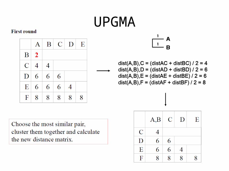
UPGMA

UPGMA

2. Determine the evolutionary distances and build

distance matrix - A simple example

1. AGGCCATGAATTAAGAATAA2. AGCCCATGGATAAAGAGTAA3. AGGACATGAATTAAGAATAA4. AAGCCAAGAATTACGAATAA

Distance Matrix

In this example the evolutionary distance is expressed as the number of nucleotide differences for each sequence pair. For example, sequences 1 and 2 are 20 nucleotides in length and have four differences, corresponding to an evolutionary difference of 4/20 = 0.2.

1 2 3 4

1 - 0.2 0.05 0.15

2 - 0.25 0.4

3 - 0.2

4 -

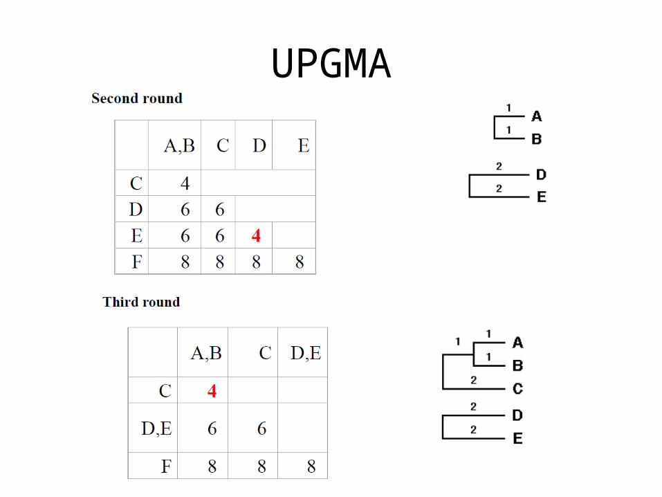
3. Phylogenetic Tree Construction example (UPGMA algorithm)

1. Pick smallest entry Dij

2. Join the two intersecting species and assign branch lengths Dij/2 to each of the nodes

DijBear Raccoon Weasel Seal

Bear - 0.26 0.34 0.29

Raccoon - 0.42 0.44

Weasel - 0.44

Seal -

Bear Raccoon

0.13 0.13

UPMGA (Michener & Sokal 1957)


DijBear Raccoon Weasel Seal

Bear - 0.26 0.34 0.29

Raccoon - 0.42 0.44

Weasel - 0.44

Seal -

3. Compute new distances to the other species using arithmetic means

365.02

44.029.0

2

38.02

42.034.0

2

)(

)(

SRSBBRS

WRWBBRW

DDD

DDD

Bear Raccoon

0.13 0.13


DijBR Weasel Seal

BR - 0.38 0.365

Weasel - 0.44

Seal -

1. Pick smallest entry Dij

2. Join the two intersecting species and assign branch lengths Dij/2 to each of the nodes

Bear Raccoon Seal

0.13

0.1825 0.1825


DijBR Weasel Seal

BR - 0.38 0.365

Weasel - 0.44

Seal -

3. Compute new distances to the other species using arithmetic means

4.03

44.042.034.0

3)(

WSWRWBBRSW

DDDD

Bear Raccoon Seal

0.13

0.1825 0.1825


DijBRS Weasel

BRS - 0.4

Weasel -

1. Pick smallest entry Dij.

2. Join the two intersecting species and assign branch lengths Dij/2 to each of the nodes.

3. Done!

Bear Raccoon Seal Weasel

0.13 0.1825

0.2 0.2

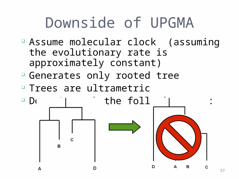
Downside of UPGMA Assume molecular clock (assuming the

evolutionary rate is approximately constant)

Generates only rooted tree Trees are ultrametric Doesn’t work the following case:

37





Neighbor-joining method

Developed in 1987 by Saitou and Nei Works in a similar fashion to UPGMA Still fast – works great for large dataset Doesn’t require the data to be

ultrametric Great for largely varying evolutionary

rates

39

How to construct a tree with Neighbor-joining method?

Step 1: Calculate sum all distance from x and divide by

(leaves – 2) Sx = (sum all Dx) / (leaves - 2)

Step 2: Calculate pair with smallest M

Mij = Distance ij – Si – Sj Step 3:

Create a node U that joins pair with lowest Mij S1U = (Dij / 2) + (Si – Sj) / 2

40

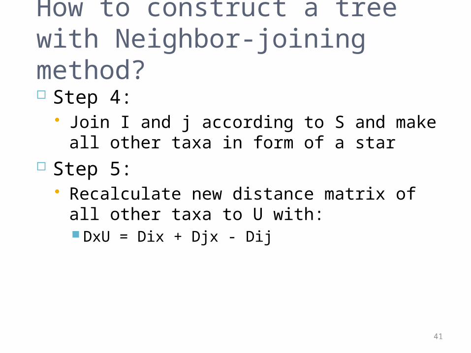
How to construct a tree with Neighbor-joining method? Step 4:

Join I and j according to S and make all other taxa in form of a star

Step 5: Recalculate new distance matrix of all other

taxa to U with: DxU = Dix + Djx - Dij

41

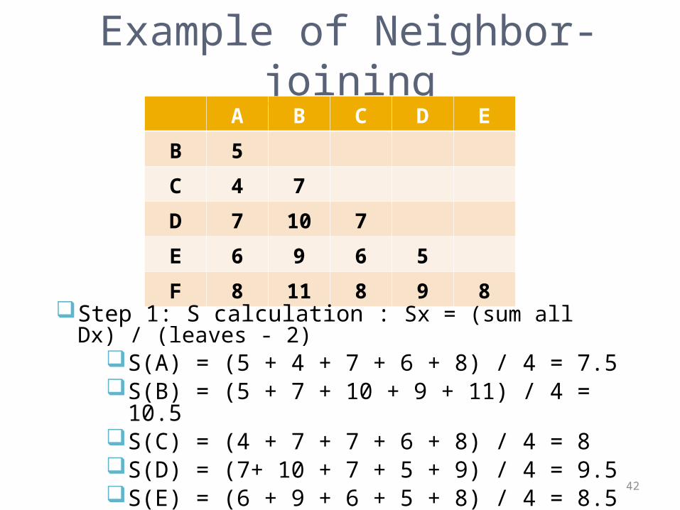
Example of Neighbor-joiningA B C D E

B 5

C 4 7

D 7 10 7

E 6 9 6 5

F 8 11 8 9 8

Step 1: S calculation : Sx = (sum all Dx) / (leaves - 2)

S(A) = (5 + 4 + 7 + 6 + 8) / 4 = 7.5S(B) = (5 + 7 + 10 + 9 + 11) / 4 = 10.5S(C) = (4 + 7 + 7 + 6 + 8) / 4 = 8 S(D) = (7+ 10 + 7 + 5 + 9) / 4 = 9.5 S(E) = (6 + 9 + 6 + 5 + 8) / 4 = 8.5 S(F) = (8 + 11 + 8 + 9 + 8) / 4 = 11

42

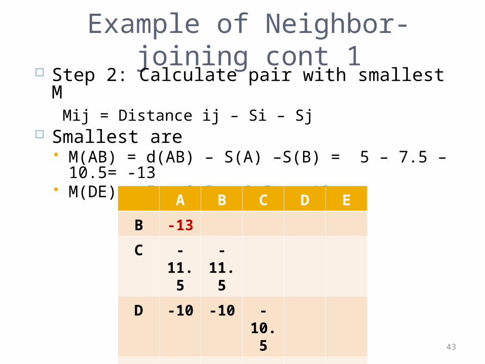
Example of Neighbor-joining cont 1

Step 2: Calculate pair with smallest M Mij = Distance ij – Si – Sj

Smallest are M(AB) = d(AB) – S(A) –S(B) = 5 – 7.5 – 10.5= -

13 M(DE) = 5 – 9.5 – 8.5 = -13

A B C D E

B -13

C -11.5

-11.5

D -10 -10 -10.5

E -10 -10 -10.5

-13

F -10.5

-10.5

-11 -11.5

-11.5

43


Step 3: Create a node US1U = (Dij / 2) + (Si – Sj) / 2

U1 joins A and B: S(AU1) = d(AB) / 2 + (S(A) – S(B)) / 2

= 5 / 2 + (7.5 - 10.5) / 2 = 1 S(BU1) = d(AB) / 2 + (S(B) – S(A)) / 2

= 5 / 2 + (10.5 – 7.5) / 2 = 4

44


Step 4: Join A and B according to S, and make all other taxa in form of a star. Branches in black are unknown length and Branches in red are known length

45


Step5: Calculate new distance matrixDxu = (Dix + Djx – Dij) / 2 d(CU) = (d(AC) + d(BC) - d(AB)) / 2

= (4 + 7 - 5) / 2 =3 d(DU) = d(AD) + d(BD) - d(AB) / 2 = 6

Same as EU and FU Then we get the new distance matrix

U1 C D E

C 3

D 6 7

E 5 6 5

F 7 8 9 846


Repeat 1 to 5 until all branches are done In this example, we will get this at the

end

47

Downside of Neighbor-joining

Generates only one possible tree Generates only unrooted tree

48





50

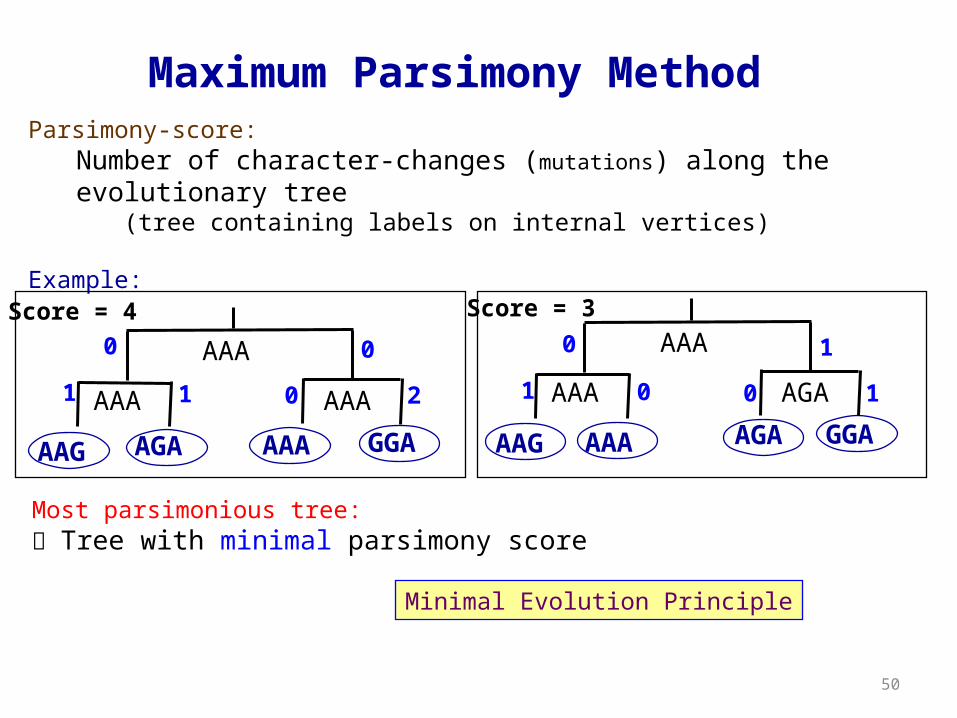
Parsimony-score:Number of character-changes (mutations) along the evolutionary tree

(tree containing labels on internal vertices)

Example:

Maximum Parsimony Method

AGA AAAAAG GGA

1 1 0 2

0 0

1 0 0 1

0 1AAA

AAA AAAAGAAAAAAG GGA

AAA

AAA AGA

Most parsimonious tree: Tree with minimal parsimony score

Score = 4 Score = 3

Minimal Evolution Principle

51

We break the problem into two:

1. Small parsimony: Given the topology find the best assignment to internal nodes

2. Large parsimony: Find the topology which gives best score

Large parsimony is NP-hard We’ll show solution to small parsimony (Fitch and Sankoff’s

algorithms)

Input to small parsimony: tree with character-state assignments to leaves

Example:

Small vs. Large Parsimony

AardvarkBisonChimp Dog Elephant

A: CAGGTAB: CAGACAC: CGGGTAD: TGCACTE: TGCGTA

52

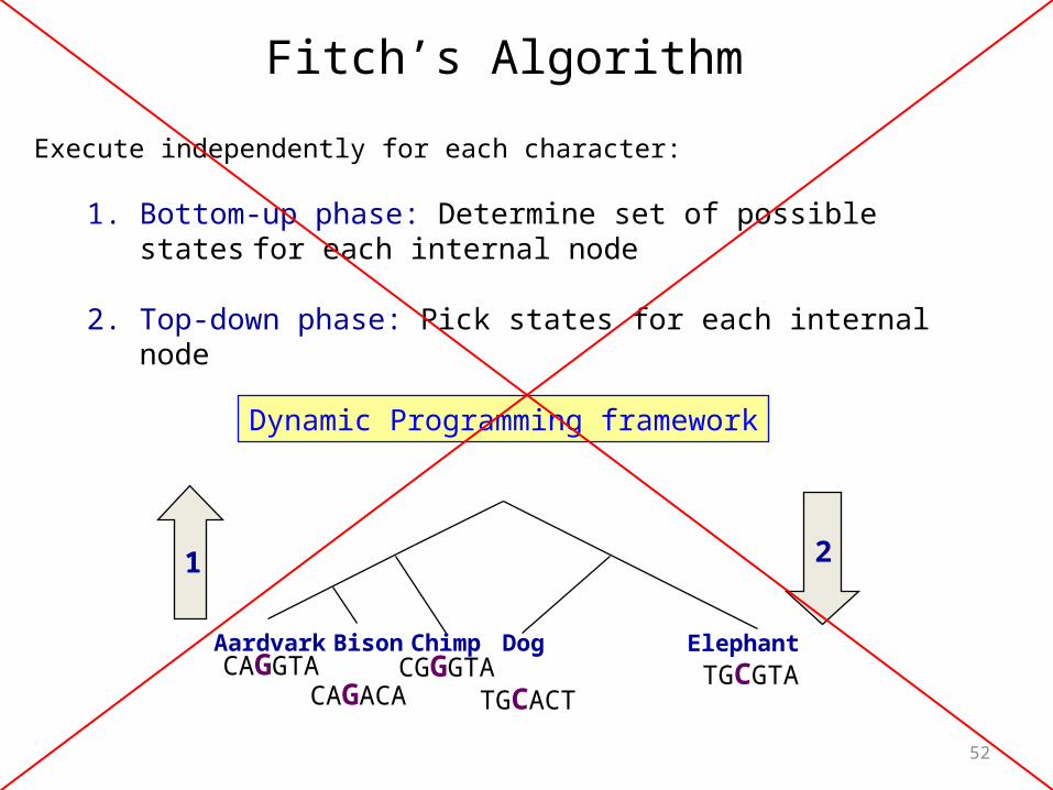
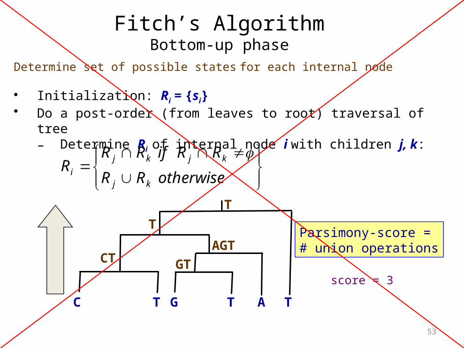
Fitch’s Algorithm

Execute independently for each character:

1. Bottom-up phase: Determine set of possible states for each internal node

2. Top-down phase: Pick states for each internal node

AardvarkBisonChimp Dog Elephant

1 2

CAGGTACAGACA

CGGGTATGCACT

TGCGTA

Dynamic Programming framework

53

Determine set of possible states for each internal node

• Initialization: Ri = {si}• Do a post-order (from leaves to root) traversal of tree

– Determine Ri of internal node i with children j, k:

Fitch’s AlgorithmBottom-up phase

Parsimony-score =# union operations

T

CT

T

C T A

otherwiseRR

RRifRRR

kj

kjkj

i

G T

AGTGT

T

score = 3

54

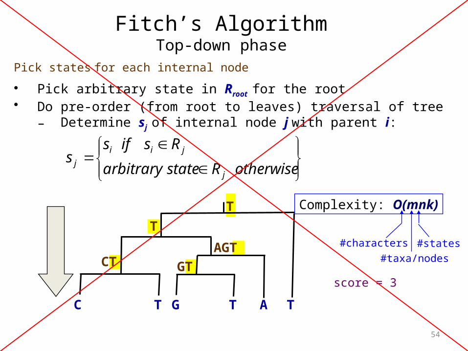
Pick states for each internal node

• Pick arbitrary state in Rroot for the root• Do pre-order (from root to leaves) traversal of tree

– Determine sj of internal node j with parent i:

Fitch’s AlgorithmTop-down phase

T

CT

T

C T AG T

AGTGT

T

otherwiseRstatearbitrary

Rsifss

j

jii

j

Complexity: O(mnk)

#characters#taxa/nodes

#states

score = 3

55

Weighted ParsimonySankoff’s algorithm

• Each mutation a↔b costs differently - S(a,b).

1. Bottom-up phase: Determine Ri(s) – cost of optimal state-assignment for subtree of i, when it is assigned state s.

2. Top-down phase: Pick optimal states for each internal node

Fitch’s algorithm as special case:• Ri – set of states which yield minimal-cost subtree of i

Same as algorithm foroptimal lifted tree alignment

(Tutorial #4)

56

Determine Ri(s) for each internal node

• Initialization: • Do a post-order (from leaves to root) traversal of tree

– Determine Ri of internal node i with children j, k:

Sankoff’s AlgorithmBottom-up phase

C T AG T T

Natural generalizationFor non-binary trees

otherwise

ssifsR i

i

0)(

),'()'(min),'()'(min)( '' ssSsRssSsRsR ksjsi

Remember pointersss’

57

Pick states for each internal node

• Select minimal cost character for root (s minimizing Rroot(s))

• Do pre-order (from root to leaves) traversal of tree:- For internal node j, with parent i, select state that produced minimal cost at i (use pointers kept in 1st stage)

Sankoff’s AlgorithmTop-down phase

C T AG T T

Complexity: O(mnk2)

#characters#taxa/nodes

#states

),'()'(min

),'()'(min)(

'

'

ssSsR

ssSsRsR

ks

jsi

58

Unweighted parsimony:

Sankoff’s algorithm:• Ri(s) - cost of optimal subtree of i, when it is assigned state s

Fitch’s algorithm:• Score(i) - cost of optimal state-assignment for subtree of i • Ri - set of optimal state-assignment for subtree of i

We need to show that:1. Optimal tree assigns node i with state from Ri.

2. Fitch’s bottom-up recursive formula for Ri. is correct:

Fitch’s Algorithmas special case of Sankoff’s algorithm

otherwiseRR

RRifRRR

kj

kjkj

i

otherwise

baifbaS

1

0),(

Check for yourselves

59

Unweighted parsimony:

• Score(i) - cost of optimal state-assignment for subtree of i • Ri - set of optimal state-assignment for subtree of i

We need to show that:1. Optimal tree assigns node i with state from Ri.

• Trivially true for the root• Assume (to the contrary) that in an optimal assignment,

some node – j is assigned sj∉Rj

otherwise

baifbaS

1

0),(

rooti

j sj∉Rj Rj(sj) ≥ Score(j)+1

By switching from sj to some s∊Rj we do not raise the parsimony-score

Why is this not the case for the weighted version?

Parsimony-score is integer

Fitch’s Algorithmas special case of Sankoff’s algorithm





Maximum likelihood

Originally developed for statistics by Ronald Fisher between 1912 and 1922

Therefore, explicit statistical model Uses all the data Tends to outperform parsimony or

distance matrix methods

61

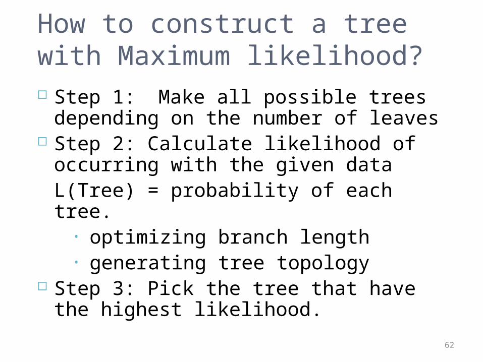
How to construct a treewith Maximum likelihood? Step 1: Make all possible trees

depending on the number of leaves Step 2: Calculate likelihood of occurring

with the given dataL(Tree) = probability of each tree.

• optimizing branch length • generating tree topology

Step 3: Pick the tree that have the highest likelihood.

62

Sounds really great?

Num of leaves

Num of possible trees

3 1

5 15

10 2027025

13 15058768725

20 8200794532637891559375

Maximum likelihood is very expensive and extremely slow to compute

63

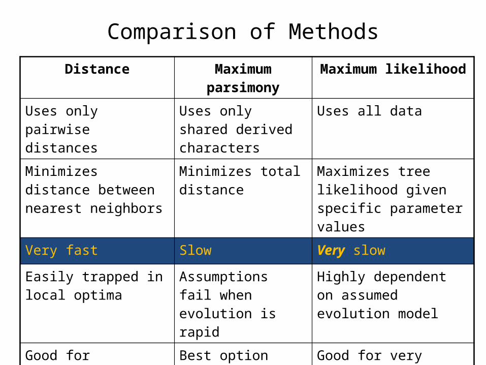
Comparison of MethodsDistance Maximum

parsimonyMaximum likelihood

Uses only pairwise distances

Uses only shared derived characters

Uses all data

Minimizes distance between nearest neighbors

Minimizes total distance

Maximizes tree likelihood given specific parameter values

Very fast Slow Very slow

Easily trapped in local optima

Assumptions fail when evolution is rapid

Highly dependent on assumed evolution model

Good for generating tentative tree, or choosing among multiple trees

Best option when tractable (<30 taxa, homoplasy rare)

Good for very small data sets and for testing trees built using other methods

Methods of evaluating trees

• Bootstrap: resample initial data set with one datum removed and replaced with another member

• Jackknife: resample initial distribution with one datum missing and not replaced

• MCMC: complex, but generates random numbers to produce a desired probability distribution with which to compare model

Phylogeny Flowchart

Difference in Methods

• Maximum-likelihood and parsimony methods have models of evolution

• Distance methods do not necessarily– Useful aspect in some circumstances

• E.g., trees built based on whole genomes, presence or absence of genes

• Religious wars over which methods to use– Most people now believe ML based methods are best: most

sensitive at large evolutionary distances – but also most time-consuming & depend on specific model of evolution used

• Most commonly used packages contain software for all three methods: may want to use more than 1 to have confidence in built tree

Phylip

• URL: http://evolution.genetics.washington.edu/phylip.html• Parsimony

– DNApenny or Protpars

• Distance– Compute distance measure using DNAdist or Protdist– Neighbor (can use NJ or UPGMA)

• ML– DNAml

http://evolution.genetics.washington.edu/phylip.html

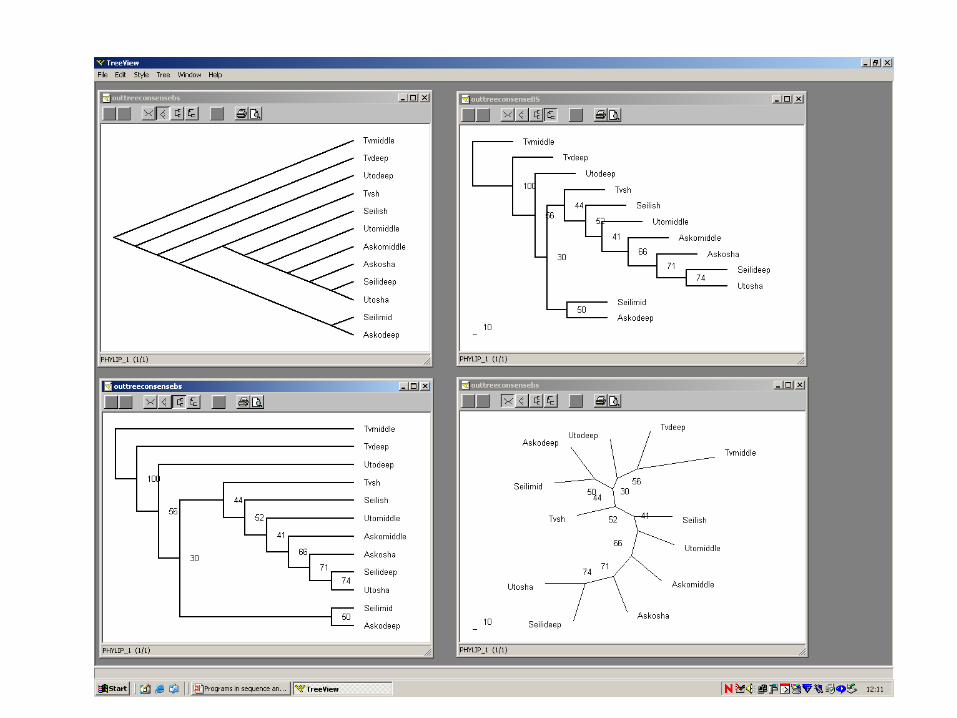
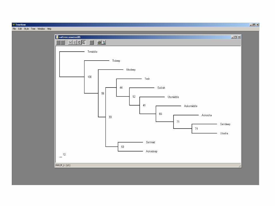
Visualising trees

• Treeview• You can change the graphic presentation of a tree (cladogram,

rectangular cladogram, radial tree, phylogram), but not change the structure of a tree

• http://homopan.wayne.edu/softwares/phoenix/index.html

http://homopan.wayne.edu/softwares/phoenix/index.html

Reference

• Mostly from Web

Documents

Presented By Dr. Shazzad Hosain Asst. Prof. EECS, NSU Phylogeny