The Impact of Climate Change on Maple Syrup Production in Ithaca

Presented By Ashley BellDr. Thomas Pfaff

Spring 2010 Whalen Symposium

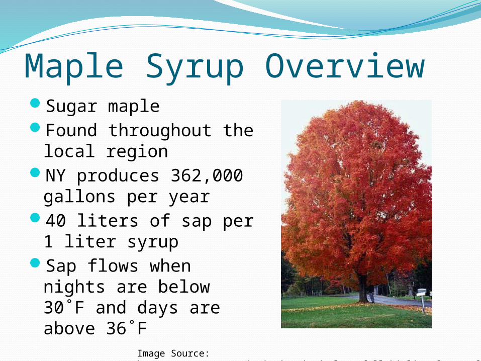
Maple Syrup OverviewSugar mapleFound throughout the local

regionNY produces 362,000 gallons

per year40 liters of sap per 1 liter

syrupSap flows when nights are

below 30˚F and days are above 36˚F

Image Source: http://www.cnr.vt.edu/dendro/dendrology/fall/biglist_frame.cfm

Climate Change Scenarios

Image source: http://sedac.ciesin.columbia.edu/ddc/sres/

A1•Rapid economic growth•Global population increases until midcentury•New and more efficient technology•Emissions increase until 2080

A2•Heterogeneous world•Continuously increasing population•Self reliance and preservation of local identities•Economic development regionally•Slow technology change•Highest emissions in 2100

B1•Sustainable development•Emphasis on global equality•Convergent world•Population peaks midcentury•Introduction of clean energies•Resource efficient technology

B2•Regional sustainability•Emphasis on local solutions to economic, social and environmental sustainability•Continuously increasing population (lower than A2)•Diverse technology change (less rapid than B1)

Current vs. Simulation Emissions

Current CO2 Levels (2010)

826.6 GtC

Project CO2 Levels (2100)

1855.3 GtC

QuestionHow will climate change effect the

maple syrup industry in Ithaca?

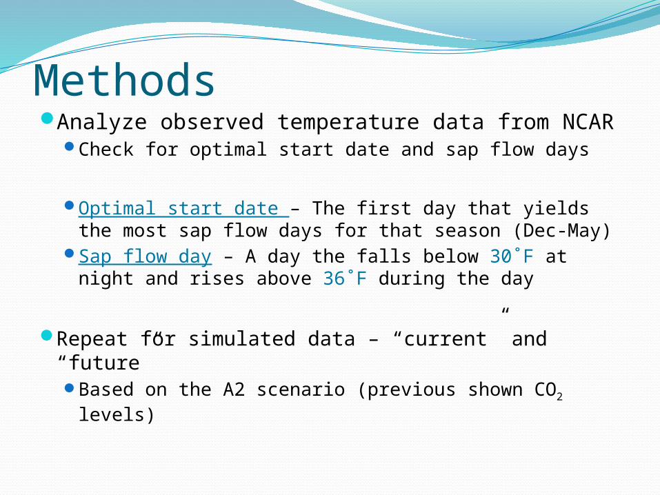
MethodsAnalyze observed temperature data from NCAR

Check for optimal start date and sap flow days

Optimal start date – The first day that yields the most sap flow days for that season (Dec-May)

Sap flow day – A day the falls below 30˚F at night and rises above 36˚F during the day

Repeat for simulated data – “current” and “future”Based on the A2 scenario (previous shown CO2 levels)

Extreme Value DistributionMaximum and minimum data – likely to be skewed Similar to normal – not everything is normal!

Density equation – Normal

Density equation – Extreme Value

Three parameters

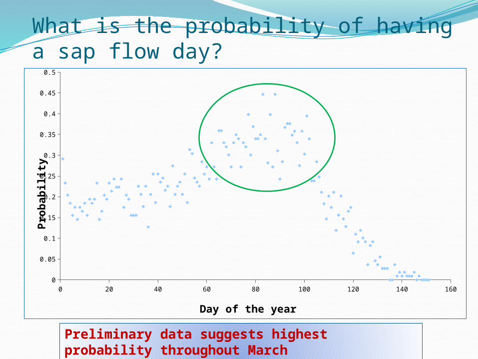
What is the probability of having a sap flow day?

0 20 40 60 80 100 120 140 1600

0.05

0.1

0.15

0.2

0.25

0.3

0.35

0.4

0.45

0.5

Day of the year

Prob

abili

ty

Preliminary data suggests highest probability throughout March

How will the start date change?Probability

Start Date50 100 150 200

Start D ate

0 .01

0 .02

0 .03

0 .04

0 .05P robab il i ty

Projected Density

Current Density

Current Median: 85 ~ Feb 23

Future Median: 77 ~ Feb 15

In the future we expect to need to start 8 days earlier

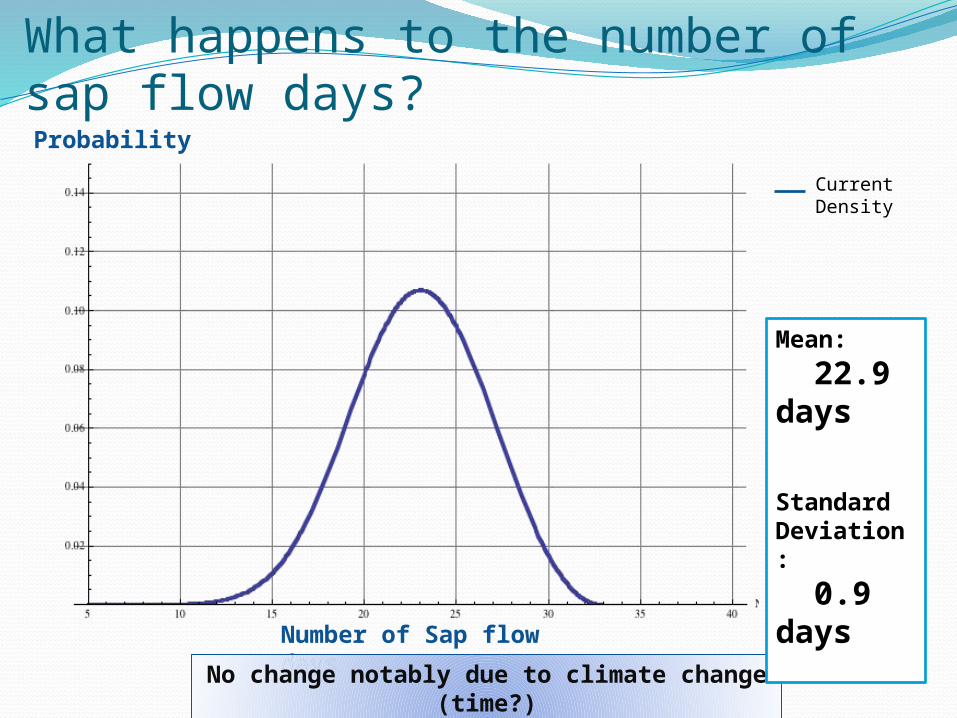
What happens to the number of sap flow days?Probability

Number of Sap flow days

No change notably due to climate change (time?)

Mean:

22.9 days

Standard Deviation:

0.9 days

Current Density

What if we start 10 days late?Probability

Number of Sap flow days

Mean (ontime):

22.9 days

Mean (late):

20.1 days

Loss -12.2%

Loss in sap flow days expected to not change in the future!

…20 days late?Probability

Number of Sap flow days

Current Density

Projected Density

Mean (ontime):

22.9 days

Mean (10 late):

20.1 days

Mean (20 late):

16.3 daysLoss- 28.8%

Mean future (20 late):

16.1 daysLoss – 29.7%

Minimal change in sap flow days from current model

ConclusionsIn the future we expect,

Earlier start date – 8 days earlierMaximum number of sap flow days for a

season (on time) not to changeLoss of of sap flow days

10 late – remain the same as now in future (Loss of 12.2%)

20 late – minimal differences between now and future (Loss of 28.8%)

Questions?