Embed Size (px)
Citation preview

Presented at CEPR-SNB conference on “Exchange Rates and External Adjustment” Zurich August 23-24, 2012
Work in progress, part of the External Balance Assessment (EBA) project of IMF Research
Department
The EBA methodology is a project of the IMF’s Research Department, under the general direction of Olivier Blanchard and Jonathan D. Ostry. The EBA Team comprises Steve Phillips, Luis Catão, Luca Antonio Ricci, Mitali Das, D. Filiz Unsal, Jungjin Lee, Marola Castillo, John Kowalski, and Mauricio Vargas. The EBA Team gratefully acknowledges comments and suggestions received, on various aspects of the project, from Joshua Aizenman, Menzie Chinn, Martin Evans, Joseph Gagnon, Eduardo Lora, Maurice Obstfeld, Dennis Quinn, and Jay Shambaugh, as well from numerous IMF colleagues. This presentation benefitted also from comments from Giuseppe De Arcangelis, Nelson Mark, Peter Pedroni, Dennis Quinn, and Kenneth West, as well as IMF seminar participants (particularly Irineu de Carvalho, Gianmaria Milesi-Ferretti and Rodrigo Valdes). This presentation should not be reported as representing the views of the IMF. The views expressed in this presentation are those of the author(s) and do not necessarily represent those of the IMF or IMF policy.

Outline Institutional context
What is new
FE versus POOL regressions
FE estimation (time dimension)
Econometric issues and methodology
Preliminary results
Misalignments (REER gaps)
Time permitting
Exploring LEVEL REER (Xsection dimension)
Further FE results

IMF: NEW ESR and EBA The IMF has a new pilot External Sector Report
http://www.imf.org/external/np/spr/2012/consult/esr/index.htm
The Research Department provides input via a new External Balance Assessment methodology (pilot, ongoing development) http://www.imf.org/external/np/res/eba/
Focuses on CA/Y, REER, NFA/Y
Previous presentation in this conference by Luis on the CA/Y leg.
This presentation is background work (IN PROGRESS) about the REER leg of EBA
It builds on and improves the previous CGER methodology: IMF OP 261 and Ricci et al. (JMCB, forthcoming) http://www.imf.org/external/pubs/cat/longres.aspx?sk=19582.0

The innovation
More determinants and similar to CA ones
More focus on policies and policy distortions
Include short term focus (business cycle, capital flows)
Positive and normative steps
Assessment based also on policy gaps from policy benchmarks
More transparency in whole process
Publish data, methodology, and final report
Focus also on individual euro countries
Criteria: theory, robustness, consistency across CA/Y and REER regressions

The innovation: more determinants and similar to CA ones In specific models, some determinants affect only REER
or CA Single good model, no REER, yet intertemporal factors
have a channel to affect CA
In static trade models, no TB, no CA, yet tradable/ nontradable stories affect REER (like Balassa-Samuelson, government consumption)
Some variables have direct effect on domestic non traded consumption prices, so CPI-REER, and not necessarily CA (unless via GE effects): Administered prices, VAT, in part also tariffs
In more general models, all variables affect both REER and CA, but to what degree?
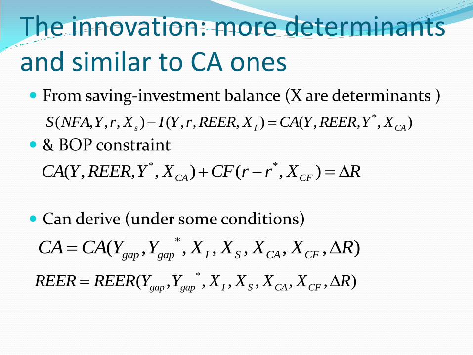
The innovation: more determinants and similar to CA ones From saving-investment balance (X are determinants )
& BOP constraint
Can derive (under some conditions)
*( , , , ) ( , , , ) ( , , , )s I CAS NFA Y r X I Y r REER X CA Y REER Y X
* *( , , , ) ( , )CA CFCA Y REER Y X CF r r X R
*( , , , , , , )gap gap I S CA CFCA CA Y Y X X X X R
*( , , , , , , )gap gap I S CA CFREER REER Y Y X X X X R

Unusual variables in literature, now in EBA Capital controls in REER, CA, and NFA regressions
Christiansen, Prati, Ricci, Tressel (2010 NBER ISOM)
Demographics in REER regressions
Rose, Supaat, and Braude (2009)
Christiansen, Prati, Ricci, Tressel (2010 NBER ISOM)
Reserves accumulation with capital controls in CA regressions
Reinhardt, Ricci, Tressel (2010); Gagnon (2012); Bayoumi et al (2012) show relevance for CA/Y

FE versus POOL regressions Most studies use FE, mainly for two reasons Most common, reliable, official, updated REER
measures are CPI based, so not comparable across countries
FE is quite the econometric standard to avoid (time-invariant) omitted variable bias
Some literature on POOL regression with LEVEL REER uses PWT based RER/REER and usually encompass mainly GDP per capita as a Balassa-Samuelson proxy (the Penn Regression)
But what about LEVEL REER regressions with more determinants?

FE versus POOL: LEVEL can help
Helps with…
Short sample, limited data availability
Structural breaks/large variation
Persistent misalignments, due for example to persistent exchange rate manipulations which are hard to measure.
Slow moving variables (e.g. VAT)
…which imply two problems
Mean REER not representative of mean equilibrium (FE tend to underestimated large persistent misalignments)
Sensitivity of mean REER (and misalignment) to small sample changes
With LEVEL, one observation of a country can be enough (if homogeneous to other countries)!

FE versus POOL: issues with POOL POOLING is GOOD only to the extent time-invariant-
omitted variable bias is limited.
Need sufficient regressors to eliminate (severity of) omitted variable bias.
And often country differences are hard to measure with variables.
NOTE that FE does not help if omitted variable is time-varying (actually FE would try to tilt fitted line to become close to actual)
For example a distortionary policy that is slowly removed over time

FE versus POOL regressions: BOTTOM LINE – 4 EXERCISES We start from (1) FIXED EFFECT panel regressions
Comparability with previous results
Immunity from standard omitted variable bias critique
We explore LEVEL REER and their cross-sectional dimension
(2) Pure cross section on time averages (XS regression)
(3) Extract fixed effects (from panel FE regressions) and regress them on time-averaged determinants, (again XS regression)
(4) POOLED regression (both time and XS dimension)

EXERCISE 1: FIXED EFFECT panel regressions The first step is to estimate the relation between
the REER and the fundamentals
where RER is IMF REER, αi is a vector of country fixed effects, Xit are the fundamentals explaining the real exchange rate, β is the vector of coefficients, and uit is the residual term.
log( )it i it itRER X u

EXERCISE 1: FIXED EFFECT panel regressions Fixed effect OLS coefficients
Standard errors corrected via the Newey-West HAC method, which accounts for heteroskedasticity both within
countries and across countries, as well as serial correlation within countries
OLS coefficients are compatible with stationarity or nonstationarity (but cointegration)
Inference Stationarity: HAC correction
Nonstationarity: cointegration tests

Econometrics and Methodology (In addition to FE/POOL)
Stationarity versus nonstationarity
Endogeneity
Serial correlation, heteroskedasticity, cross-sectional dependence
Dynamics
Heterogeneity
Issues addressed mainly as robustness

E&M: stationarity? Tests of stationarity v/s nonstationarity are inconclusive
Most literature used to find REER nonstationarity in the past
In our sample: standard PUR tests find REER stationary (also in recent IMF work
Cashin et al IMF/WP/09/78)
PUR test based on cross-sectional dependence (CSD) (Pesaran 2007), find REER nonstationary
But CSD should be limited for vars relative to trading partners
OLS COEFFICIENTS are ok in both cases If stationary, HAC corrected standard errors are relevant
In nonstationary, inference is based on cointegration test. Stationary variables do not harm cointegrating relationship
ARDL would need heterogenous dynamics and loose degrees of freedom: only a few variables could be investigated

E&M: endogeneity
In absence of clear instruments, we have two options:
1) lag potentially endogenous variables (in OLS)
2) or instrument variables via 2SLS with lags of endogenous as well as possible instruments (as robustness)

E&M: correcting standard errors
Under the presumption of stationary variables, inference is based on corrected standard errors with the Newey-West HAC method, which accounts for heteroskedasticity—both within countries and across countries—as well as serial correlation within countries.
An alternative correction for cross-sectional dependence (Kraay and Driscoll 1998) does not change much the results (sign that CDS is not serious)

E&M: dynamics homogeneous dynamics generate biased estimates of
long run,
heterogenous dynamics allow only a few variables (as in a country by country regression), while we need many regressors
Robustness: we check homogeneous long run and heterogenous dynamics w/ PMGE, which allows only a few variables. Most robust are:
In long run: health expenditure, capital controls, output gap, financial home bias, terms of trade, growth forecast.
In short run: VIX terms

E&M: heterogeneity
Slope homogeneity is an assumption
in part essential (not enough observations for country by country regressions)
in part addressed via variable construction relative to trading partners
also addressed via interaction terms.
In POOL, several regressors helps addressing the heterogeneity of the constant, and helps us understanding it.

Sample 42 countries
Including the 11 major euro area countries individually
1990-2010
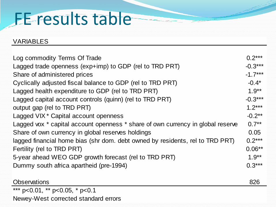
FE results table VARIABLES
Log commodity Terms Of Trade 0.2***
Lagged trade openness (exp+imp) to GDP (rel to TRD PRT) -0.3***
Share of administered prices -1.7***
Cyclically adjusted fiscal balance to GDP (rel to TRD PRT) -0.4*
Lagged health expenditure to GDP (rel to TRD PRT) 1.9**
Lagged capital account controls (quinn) (rel to TRD PRT) -0.3***
output gap (rel to TRD PRT) 1.2***
Lagged VIX * Capital account openness -0.2**
Lagged vox * capital account openness * share of own currency in global reserve 0.7**
Share of own currency in global reserves holdings 0.05
lagged financial home bias (shr dom. debt owned by residents, rel to TRD PRT) 0.2***
Fertility (rel to TRD PRT) 0.06**
5-year ahead WEO GDP growth forecast (rel to TRD PRT) 1.9**
Dummy south africa apartheid (pre-1994) 0.3***
Observations 826
*** p<0.01, ** p<0.05, * p<0.1
Newey-West corrected standard errors

FE results Commodity terms of trade has a positive sign. The size of the
coefficient is somewhat lower than standard literature, in part due to the richer model (other variables such as the fiscal balance may capture part of the effect of commodity prices).
Trade openness (lagged) has a negative sign. Average exports and imports to GDP is a proxy for trade liberalization, which lowers the domestic price of tradable goods, thus depreciating the CPI-based REER. As a change in the exchange rate affects differently the numerator and denominator of openness, this is indicator is lagged.
The share of administered prices has a negative sign (as administered prices are generally imposed to lower prices). Available only for a few transition economies (for the rest it is assumed to be 0). A decrease in the share of administered prices by 1 percent is associated with a 1½ percent appreciation.

FE results General government cyclically adjusted balance to
GDP is negative (in line with positive in the CA regressions): when the balance increases by 1 percentage point of GDP, the REER depreciates by 0.4%.
Health expenditure to GDP (lagged) has a positive sign (consistent with a negative sign in the CA regressions): an increase in health expenditure by 1 percentage point of GDP is associated with a 2 percent appreciation.
Capital account controls (lagged) is negative (consistent with a positive sign in the CA regressions), and with the idea that this variable mainly captures the effect of capital controls on inflows (lower ability to borrow and run current accounts deficits, and a more depreciated exchange rate).

FE results The output gap has a positive coefficient (consistent with
a negative sign in the CA regression): an increase in the output gap by 1 percentage point of GDP is associated with an appreciation somewhat above 1 percent.
VIX/VOX (indicator of global risk aversion), interacted with capital account openness (lagged).
For non reserve currency countries, the effect is negative (depreciation) associated with the need to generate a CA surplus when global risk aversion increases and access to credit becomes more difficult. The effect is stronger the more open the capital account is.
For reserve currency countries the effect is in the opposite direction, and appreciates the currency.

FE results Financial home bias (lagged) has positive sign. It is
calculated as the share of domestic debt owned by residents. Preference for holding domestic assets should appreciate the REER. (Other variables in the regression tend to capture international investor preference for the country assets , which would have the opposite effect on the exchange rate). The variable is lagged, as changes in the exchange rate can affect the indicator purely from a composition effect (foreigners’ share is more likely to be denominated in foreign currency).
Fertility has a positive sign: the higher the fertility rate, the higher the share of inactive population, which is associated with lower net saving, and more appreciated real exchange rates. The work of Rose, Supaat, and Braude (2009) suggests that fertility is the best proxy for demographic factors in real exchange rate regressions.

FE results Forecast GDP growth (5-year ahead) has a positive
coefficient, consistent with the negative coefficient found in the CA regression (faster growth is associated with a weaker current account and a more appreciated real exchange rate).
Dummy for South Africa until 1994, absorbing a significant structural break at the end of the apartheid This has very little effect on results, even for South Africa.

FE results: extensions and robustness Traditional variables
Productivity mainly cross-section
NFA: binding constraint (negative NFA or capital controls)
Government consumption: health exp. chosen for consistency
Fiscal balance captures also opposite confidence factors
Reserve intervention: right sign but not robust
Interaction with:
Capital controls (fertility, output gap)
Exchange rate regime (growth forecast, financial home bias)
Other variables with time pattern
Interest rate differential, financial development,
Other variables with cross-sectional pattern
Institutions, VAT

Misalignments and policy gaps Consider Fit fundamentals, Pit policy variables, and P*it
optimal levels of policy variables
Can decompose REER as:
REER norm policy gap regression residual
Total EBA GAP
Then, adjust residual and Total EBA gap for multilateral consistency, if necessary
log( )it i it itRER X u
log( )it i it it itRER F P u
* *log( ) ( )it i it it it it itRER F P P P u

Misalignments and policy gaps Zero residual does not mean OK
REER may fit perfectly with existing policies, but policies may need to change
Adjusting for policy gaps informs on the level of REER that would prevail in the absence of these policy gaps
A country policy at optimal level does not mean zero policy gap
Note that both Pit and P*it are relative to other countries,
hence, a country may have a policy gap even if its policies are at optimal level (think of fiscal policy now)

Misalignment and policy gaps: multilateral consistency Important to ensure that the weighted average of residuals
are zero in each year (multilateral consistency). To a large extent consistency is achieved via careful
construction of the variables relative to the trading partner weighted average of the same variable.
As standard in CGER (see Occasional Paper 167, Chapter 7), multilateral consistency is then ensured by adjusting each exchange rate residual by the global weighted average of residuals.
The weights are given by the eigenvector associated with the unit eigenvalue of the trade weights matrix.
The necessary adjustment is tiny (less than 1 percent), which indicates proper variable construction and good overall fit.

The road ahead
Further attention to fiscal and reserve intervention
Missing variables?
More policy measures?
Exploring LEVEL regressions


![camille pedroni [camille.pedroni@ulb.ac.be] introduction](https://img.pdfslide.us/doc/110x75/617b63da70d239624d6954ba/camille-pedroni-ulbacbe-introduction-.jpg)