Presentazione di PowerPoint - Politecnico di Milanobascetta.deib.polimi.it/images/3/34/CONTAUT_MEC-Lect11.pdf · 16. Prof. Luca Bascetta ... Consider a 2- d.o.f. planar manipulator

Prof. Luca Bascetta ([email protected])

Politecnico di MilanoDipartimento di Elettronica, Informazione e Bioingegneria

Automatic ControlIndustrial robotics

mailto:[email protected]

Prof. Luca BascettaProf. Luca Bascetta

Industrial robots (I)

The International Organization for Standardization (ISO) gives the following definition of an industrial robot:

“ an automatically controlled,reprogrammable, multipurpose,manipulator programmable in threeor more axes, which may be eitherfixed in place or mobile for use inindustrial automation applications ”

A robot is an electro-mechanicalsystem guided by a control unit, it isnot only mechanics, but electronics,software, control, etc.

2


Industrial robots (II) 3

COMAU Smart NJ 4 90 COMAU C5G

Mechanical chain, actuatorsand sensors

Control unit


Industrial robots (III)

The mechanical chain is constituted by a sequence of links connected by joints.

The first body of the chain is the baseof the robot and is usually fixed to thefloor, a wall or the ceiling.

The last body is the end-effector onwhich the tool to execute the task ismounted.

The mechanical chain is usuallycomposed by six links:• the first three set the position• the last three set the orientationof the end-effector.

4


Industrial robots (IV) 5

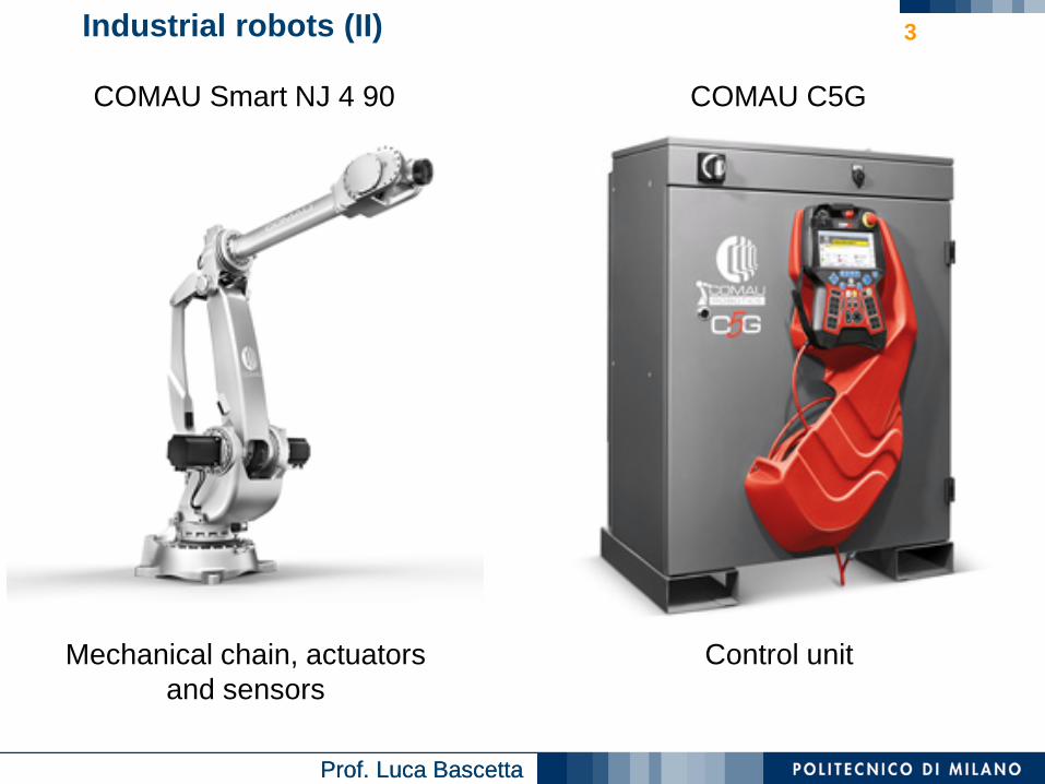
Control unit• MMI• power units• motion planning• control

Teach pendant• programming interface


Industrial robots (V) 6

Small payload robots (from 5 to 16 Kg)


Industrial robots (VI) 7

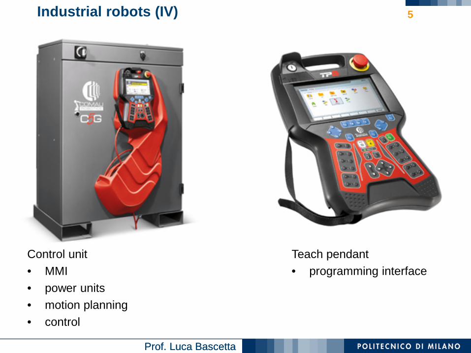
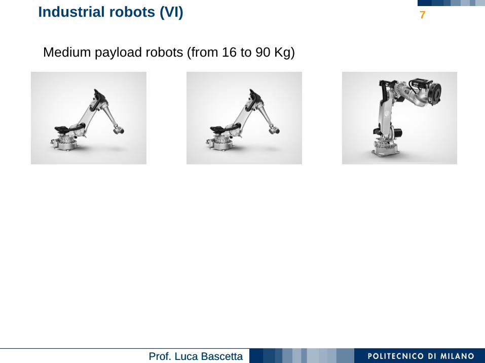
Medium payload robots (from 16 to 90 Kg)


Industrial robots (VII) 8

High payload robots (from 110 to 220 Kg)


Industrial robots (VIII) 9

High speed pick and place robots


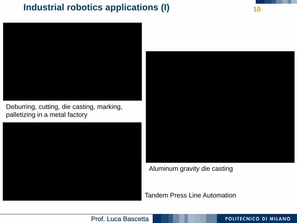
Industrial robotics applications (I) 10

Deburring, cutting, die casting, marking,palletizing in a metal factory

Aluminum gravity die casting

Tandem Press Line Automation


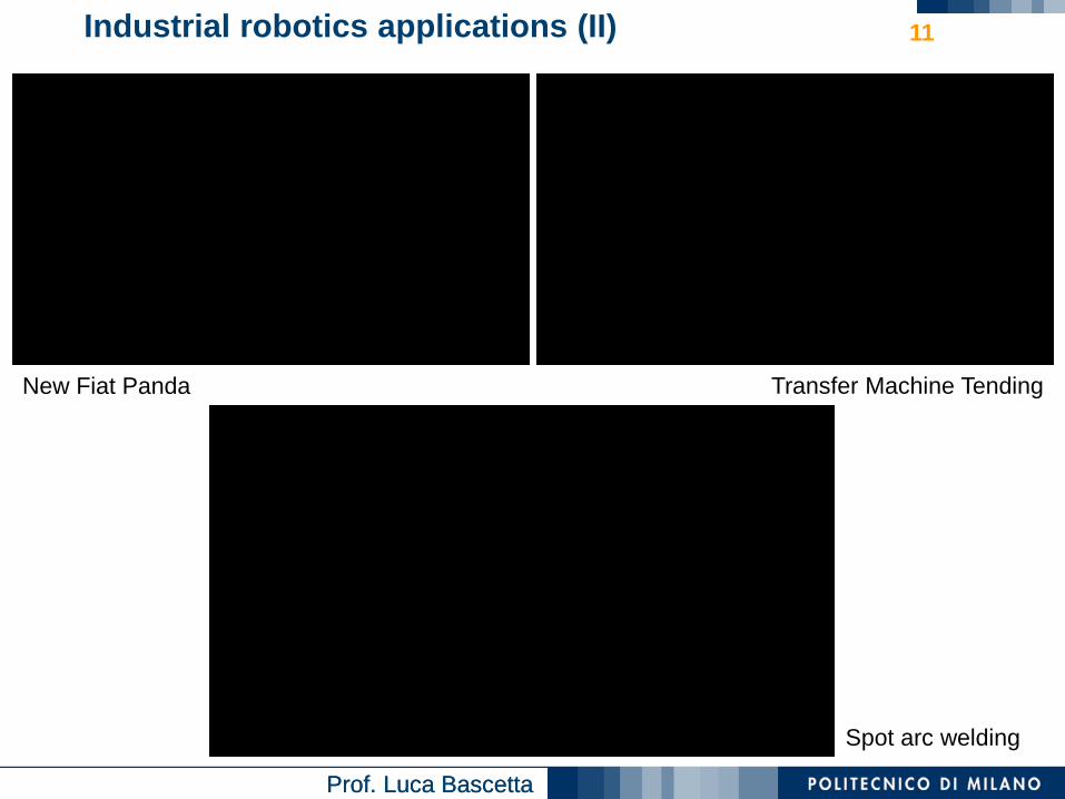
Industrial robotics applications (II) 11

New Fiat Panda Transfer Machine Tending

Spot arc welding


Redundant and dual-arm robots 12

MotomanSIA 10D

Kuka LWR


Motion control and robotics

We will now consider the typical motion control problems of industrial robotics as a case study.

We will concentrate on the following topics:• robot modelling

• kinematics• dynamics

• motion planning• joint space planning• Cartesian space planning

• closed-loop control• decentralized control• centralized control

13


Forward and inverse kinematics (I)

Forward kinematics refers to the problem of computing end-effector position and orientation, given joint positions.

A systematic procedure based on DH parameters and rotation or homogenous matrices can be introduced.

14


Forward and inverse kinematics (II)

Inverse kinematics refers to the problem of computing joint positions, given end-effector position and orientation.

Inverse kinematics is a far more complex problem, it can be solved using ad-hoc algorithms or approximate methods.

15


Forward and inverse kinematics (II)

Differential kinematics refers to the relation between joint velocities and end-effector linear and angular velocities.

For a given robot configuration the relation between joint velocities and end-effector velocities is linear and is represented by the Jacobian matrix.

16


Forward and inverse kinematics – Example

Consider a 2-d.o.f. planar manipulatorForward kinematics

Inverse kinematics

Differential kinematics

17


Manipulator dynamics (I)

Forward dynamics is a relation between joint motor torques and joint (or end-effector) motion (position and velocity).

18


Manipulator dynamics (II)

To devise the dynamic model of a manipulator we can follow two different ways.

Euler-Lagrange method• the manipulator is described as a chain of rigid bodies subject to holonomous

motion constraints• a set of generalized coordinates is selected (joint coordinates)• for each coordinate a Lagrange equation is written

Newton-Euler method• for each rigid body force and momentum balances are

written, considering interaction forces/momenta withother rigid bodies

• a set of computationally efficient recursive relationsis obtained

19


Manipulator dynamics (III)

The dynamic model is described by 𝑛𝑛 second order differential equations.If 𝐪𝐪 is the vector of joint variables we get

Joint torquesGravitational termsCentrifugal and Coriolis termsInertial termsThe inertia matrix 𝐁𝐁 𝐪𝐪 is a symmetric an positive definite matrix

20


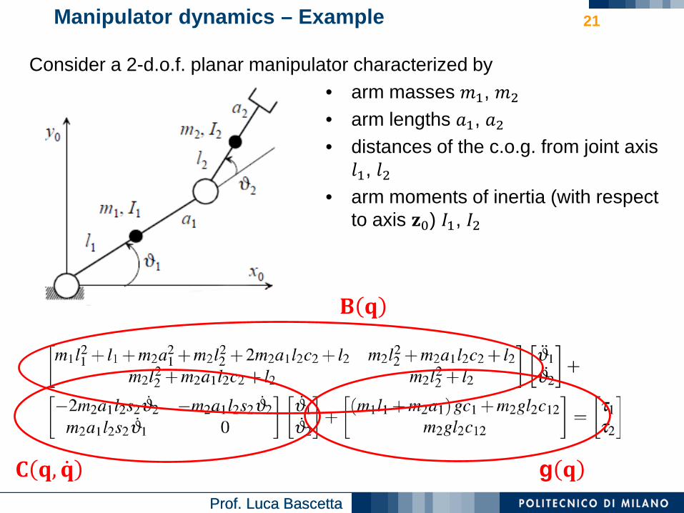
Manipulator dynamics – Example

Consider a 2-d.o.f. planar manipulator characterized by• arm masses 𝑚𝑚1, 𝑚𝑚2

• arm lengths 𝑎𝑎1, 𝑎𝑎2• distances of the c.o.g. from joint axis

𝑙𝑙1, 𝑙𝑙2• arm moments of inertia (with respect

to axis 𝐳𝐳0) 𝐼𝐼1, 𝐼𝐼2

21

𝐁𝐁 𝐪𝐪

𝐂𝐂 𝐪𝐪, �̇�𝐪 g 𝐪𝐪


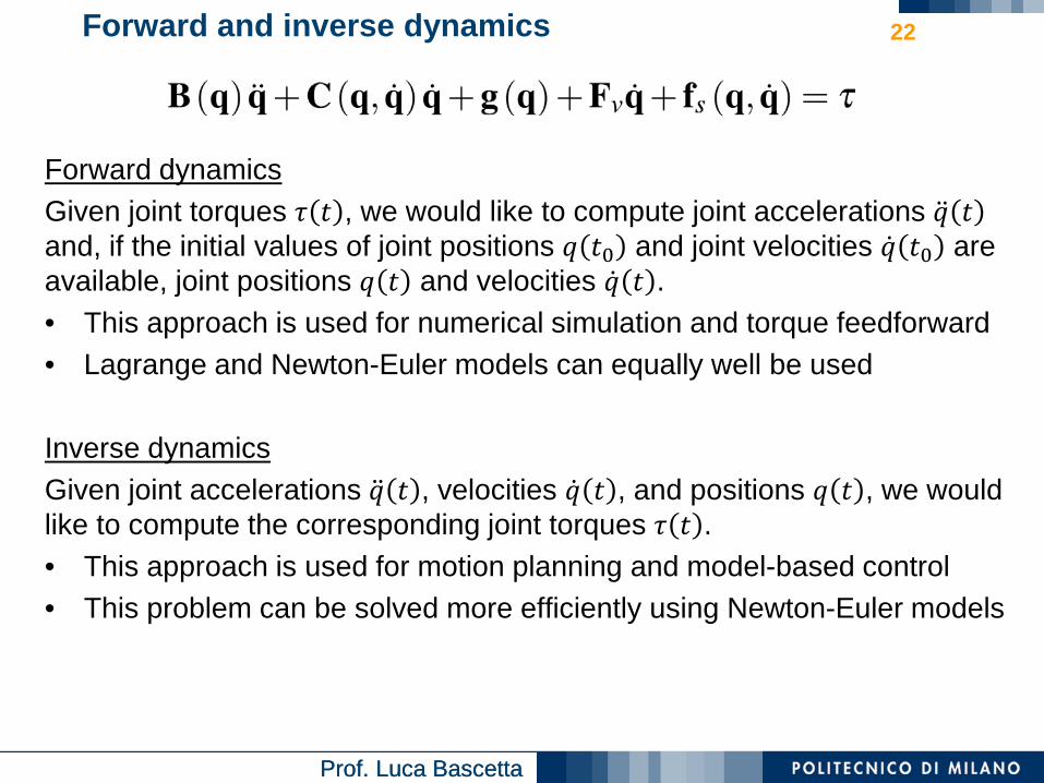
Forward and inverse dynamics

Forward dynamicsGiven joint torques 𝜏𝜏 𝑡𝑡 , we would like to compute joint accelerations �̈�𝑞 𝑡𝑡and, if the initial values of joint positions 𝑞𝑞 𝑡𝑡0 and joint velocities �̇�𝑞 𝑡𝑡0 are available, joint positions 𝑞𝑞 𝑡𝑡 and velocities �̇�𝑞 𝑡𝑡 .• This approach is used for numerical simulation and torque feedforward• Lagrange and Newton-Euler models can equally well be used

Inverse dynamicsGiven joint accelerations �̈�𝑞 𝑡𝑡 , velocities �̇�𝑞 𝑡𝑡 , and positions 𝑞𝑞 𝑡𝑡 , we would like to compute the corresponding joint torques 𝜏𝜏 𝑡𝑡 .• This approach is used for motion planning and model-based control• This problem can be solved more efficiently using Newton-Euler models

22


Motion planning (I)

Let’s first introduce some definitions.

Path, is a sequence of points defining a curve in a given space (joint space, Cartesian space, etc.) a moving object should follow.

Motion law, is a continuous function that defines the relation between time and position of a moving object along the path.

Trajectory, is the path that a moving object follows as a function of time (i.e., it is a path together with a motion law).

Solving a motion planning problem means determining a trajectory that is used as reference signal for position/velocity control loops.A motion planning problem can be solved either in joint space or in Cartesian space.

23


Motion planning (II)

Cartesian space trajectory planning, we determine the path (position and orientation) of the robot end-effector in Cartesian space and the motion law.• It is the most natural way to describe a task• Constraints along the path can be easily taken into account• Singular configurations and redundant degrees of freedom make

Cartesian planning more complex• Inverse kinematics has to be computed online

Joint space trajectory planning, we determine the path in terms of joint coordinates and the motion law.• Singular configurations do not represent a problem• We do not need to compute inverse kinematics online• It is used when the motion in Cartesian space is not of interest (i.e., there

is no coordination among the motion of the joints, or the goal is only to take the arm to a final configuration)

24


Motion planning (III)

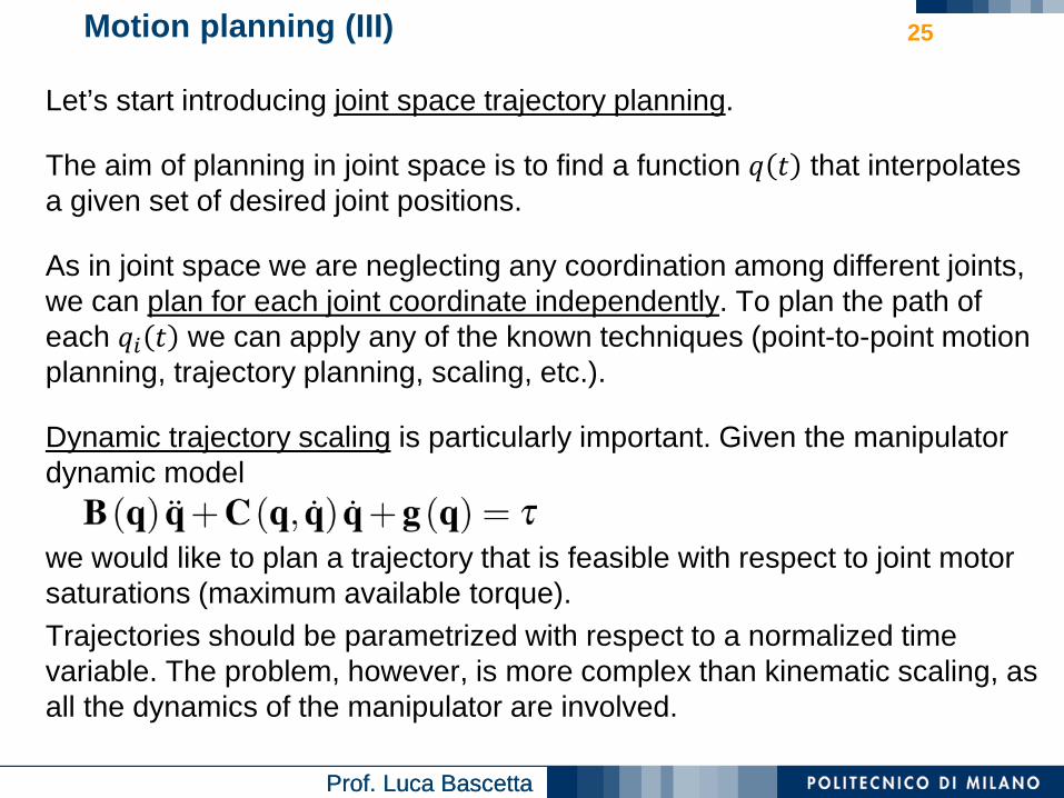
Let’s start introducing joint space trajectory planning.

The aim of planning in joint space is to find a function 𝑞𝑞 𝑡𝑡 that interpolates a given set of desired joint positions.

As in joint space we are neglecting any coordination among different joints, we can plan for each joint coordinate independently. To plan the path of each 𝑞𝑞𝑖𝑖 𝑡𝑡 we can apply any of the known techniques (point-to-point motion planning, trajectory planning, scaling, etc.).

Dynamic trajectory scaling is particularly important. Given the manipulator dynamic model

we would like to plan a trajectory that is feasible with respect to joint motor saturations (maximum available torque).Trajectories should be parametrized with respect to a normalized time variable. The problem, however, is more complex than kinematic scaling, as all the dynamics of the manipulator are involved.

25


Motion planning (IV)

Consider now Cartesian space trajectory planning.

First, we need to introduce a way to specify the path in Cartesian space.Let’s start from the representation of the end-effector position. We can represent the path using a parametric curve, parameterized using the natural coordinate 𝑠𝑠: 𝐩𝐩 = 𝐩𝐩 𝑠𝑠 .

26


Motion planning – Example

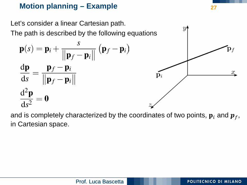
Let’s consider a linear Cartesian path.The path is described by the following equations

and is completely characterized by the coordinates of two points, 𝐩𝐩𝑖𝑖 and 𝒑𝒑𝑓𝑓, in Cartesian space.

27


Motion planning (V)

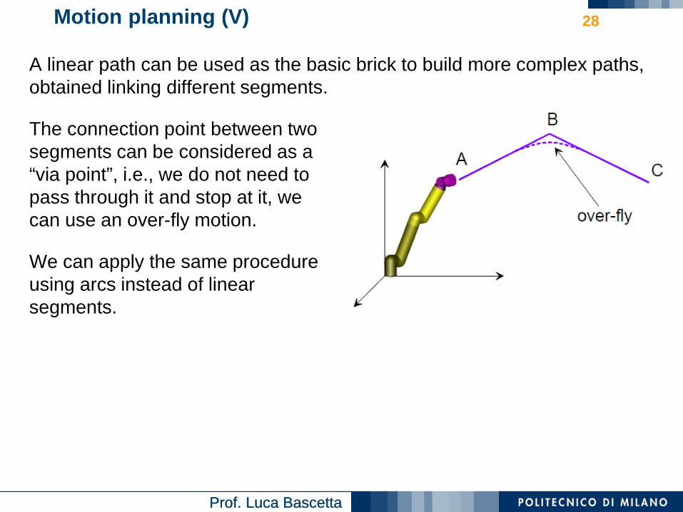
A linear path can be used as the basic brick to build more complex paths, obtained linking different segments.

The connection point between twosegments can be considered as a“via point”, i.e., we do not need topass through it and stop at it, wecan use an over-fly motion.

We can apply the same procedureusing arcs instead of linearsegments.

28


Motion planning (VI)

We have seen how to specify the end-effector position in Cartesian space, using parametric curves. How can we introduce the motion law?

The motion law can be introduced on the natural coordinate 𝑠𝑠 = 𝑠𝑠 𝑡𝑡 .In fact, we have

where �̇�𝑠 is the absolute value of the velocity along the path.As the natural coordinate is a scalar quantity, we can use all the methods introduced to plan the trajectory of a motor (polynomial, harmonic, trapezoidal trajectories).

From a conceptual point of view, the same procedure can be used to plan the end-effector orientation, once a suitable representation of the orientation has been selected.

29


Robot programming

The controller of an industrial robot is equipped with a specific programming language (PDL2 for Comau robots, RAPID for ABB robots, etc.) that can be used to program robot tasks.A software simulator (Robosim Pro for Comau robots, RobotStudio for ABB robots, etc.) is usually available as well, to help off-line programming and testing.There are three basic methods for programming:• teach method, a teach pendant is used to manually drive the robot to the

desired locations and store them. The logic of the program can be generated using the robot programming language

• lead through, the robot is programmedbeing physically moved through the task byan operator, the controller simply recordsthe joint positions at a fixed time intervaland then plays them back

• off-line programming, the robot is programmedusing CAD data and a suitable software

30


Robot programming – Example

This program moves pieces from a feeder to a table or a discard bin, according to some digital input signals.

PROGRAM packVAR

home, feeder, table, discard : POSITIONBEGIN CYCLE

MOVE TO homeOPEN HAND 1WAIT FOR $DIN[1] = ON

-- signals feeder readyMOVE TO feederCLOSE HAND 1IF $DIN[2] = OFF THEN

-- determines if good partMOVE TO table

ELSEMOVE TO discard

ENDIFOPEN HAND 1

-- drop part on table or in binEND pack

31

1 – feeder, 2 – robot, 3 – discard bin, 4 – table


Motion control (I)

Motion control is usually accomplished at joint level using closed-loop control strategies.The following architecture is usually adopted

where• trajectory planning and kinematic inversion are executed offline, or online

with a reduced cycle rate (~100 𝐻𝐻𝐻𝐻)• servo loops are executed online and in real-time with a faster cycle rate

(≥ 1 𝑘𝑘𝐻𝐻𝐻𝐻)

32


Motion control (II)

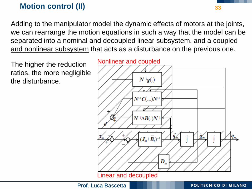
Adding to the manipulator model the dynamic effects of motors at the joints, we can rearrange the motion equations in such a way that the model can be separated into a nominal and decoupled linear subsystem, and a coupled and nonlinear subsystem that acts as a disturbance on the previous one.

The higher the reductionratios, the more negligiblethe disturbance.

33

Nonlinear and coupled

Linear and decoupled


Motion control (III)

Exploiting the previous result, we can develop the independent joint controlstrategy, the most common solution in commercial industrial robots.

We can neglect the coupling effects, considering them as disturbances, and control the manipulator motion with 𝑛𝑛 independent SISO loops.

The design of the control system of each SISO loop can be faced using the techniques we have introduced for the position and velocity control of a servomechanism.

This control architecture is strongly based on the decoupling effect due to the presence of transmissions characterized by high reduction ratios.

Though this is the most common solution in commercial products, in the last decade robot manufacturers have started introducing more complex control architectures.

34


Motion control (IV)

The first improvement to the standard independent joint control architecture was the introduction of a feedforward action based on the manipulator dynamic model.The dynamic model, fed by position, velocity and acceleration references, is used to compute and compensate the disturbances.

The feedforward compensation is usually adopted to compensate only part of the disturbances (gravitational torque and diagonal terms of the inertia matrix).

35


Motion control (V)

Another decentralized control architecture is the PD control with gravity compensation.This control scheme is characterized by two diagonal gain matrices 𝐊𝐊𝑃𝑃 and 𝐊𝐊𝐷𝐷.

It can be shown that with a rigid manipulator and a perfect compensation of gravitational torques, the equilibrium (characterized by zero steady-state error) of the closed-loop system is globally asymptotically stable.

36

Robot model


Motion control (VI)

A centralized architecture, instead, can be devised using the manipulator dynamic model to compensate all the nonlinear couplings between the joints.

37

Robot model


Motion control (VII)

The equations that describe theclosed-loop system are

Assuming a perfect compensation of the nonlinear terms we get

and defining the error 𝐞𝐞 = 𝐪𝐪𝑑𝑑 − 𝐪𝐪

Thanks to the compensation of the nonlinear terms, the PD regulator is designed on a system constituted by 𝑛𝑛 decoupled double integrator systems.The dynamics of the error system can be arbitrarily assigned using PD gains 𝐊𝐊𝑃𝑃 and 𝐊𝐊𝐷𝐷.

38

Robot model

Documents

Presentazione di PowerPoint - Politecnico di Milanobascetta.deib.polimi.it/images/3/34/CONTAUT_MEC-Lect11.pdf · 16. Prof. Luca Bascetta ... Consider a 2- d.o.f. planar manipulator