Embed Size (px)
Citation preview

Presentation ByMichael Tao and Patrick Virtue

Agenda
• History of the problem• Graph cut background• Compute graph cut• Extensions• State of the art• Continued Work
Agenda
• History of the problem• Graph cut background• Compute graph cut• Extensions• State of the art• Continued Work

Image Segmentation : History• Computer Vision Problem Since 1970’s• Two Key Problems: • Edge detection• Image segmentation

Image Segmentation : History• Edge detectors, descriptors• 1980 – Canny Edge Detector• No contours- just edges
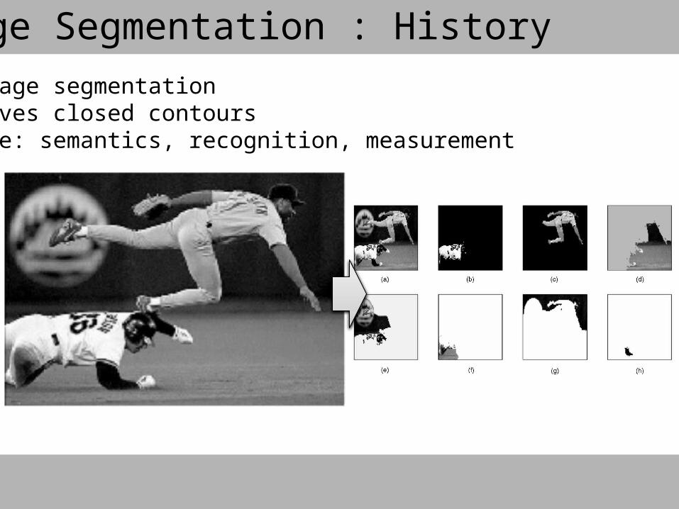
Image Segmentation : History• Image segmentation• Gives closed contours• Use: semantics, recognition, measurement
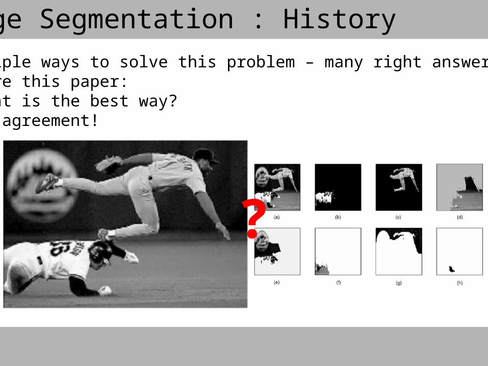
Image Segmentation : History• Multiple ways to solve this problem – many right answers• Before this paper:
- What is the best way?- No agreement!
?

Agenda
• History of the problem• Graph cut background• Compute graph cut• Extensions• State of the art• Continued Work
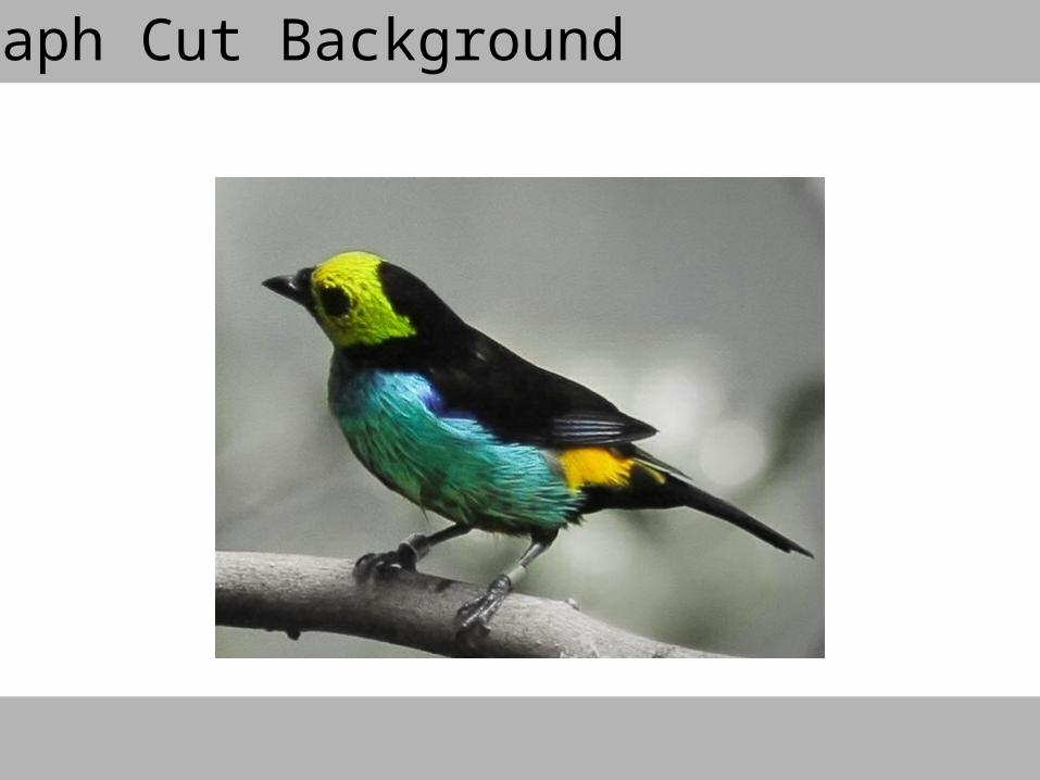
Graph Cut Background
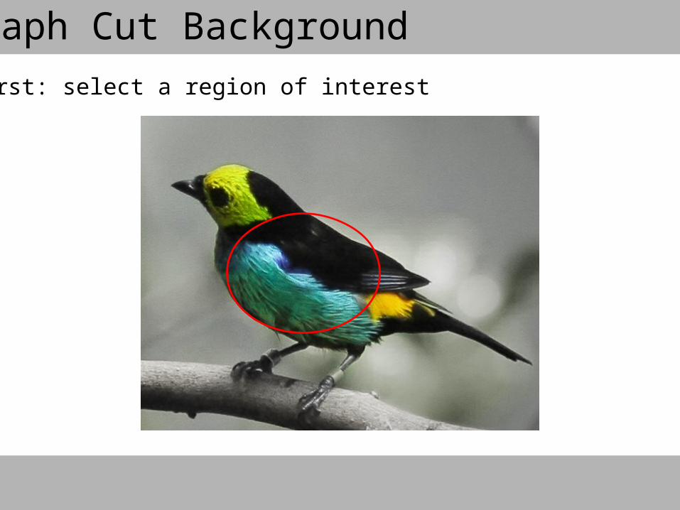
• First: select a region of interest
Graph Cut Background
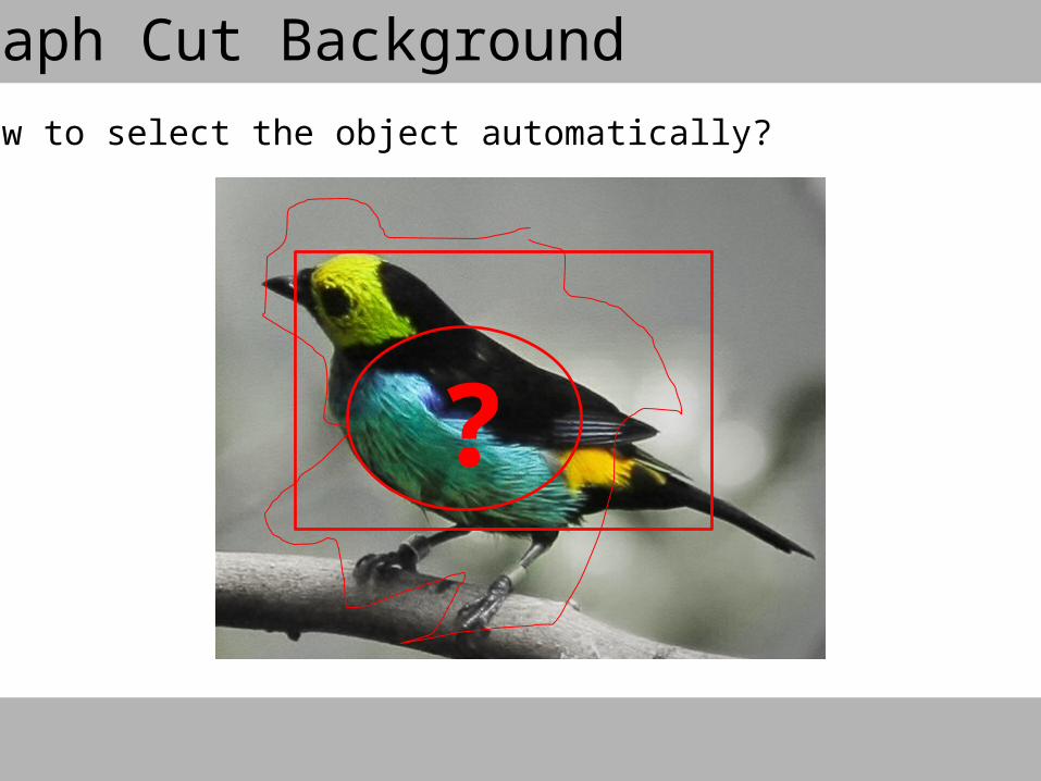
• How to select the object automatically?
?
Graph Cut Background

• We care about two terms: graph and cuts
?
Graph Cut Background
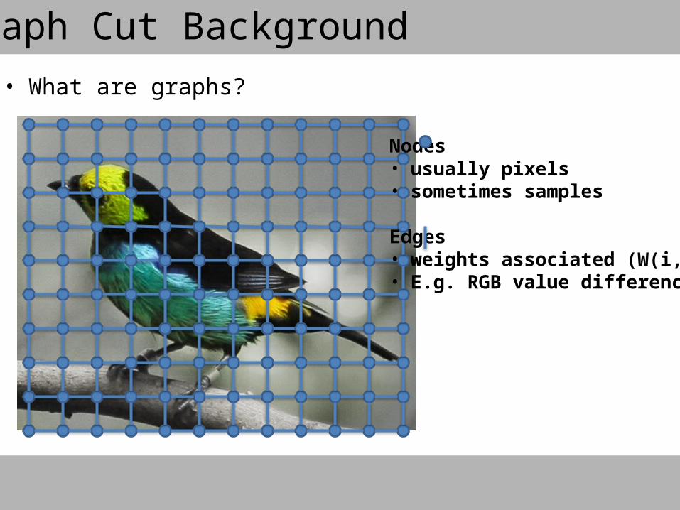
Graph Cut Background• What are graphs?
Nodes• usually pixels• sometimes samples
Edges• weights associated (W(i,j))• E.g. RGB value difference
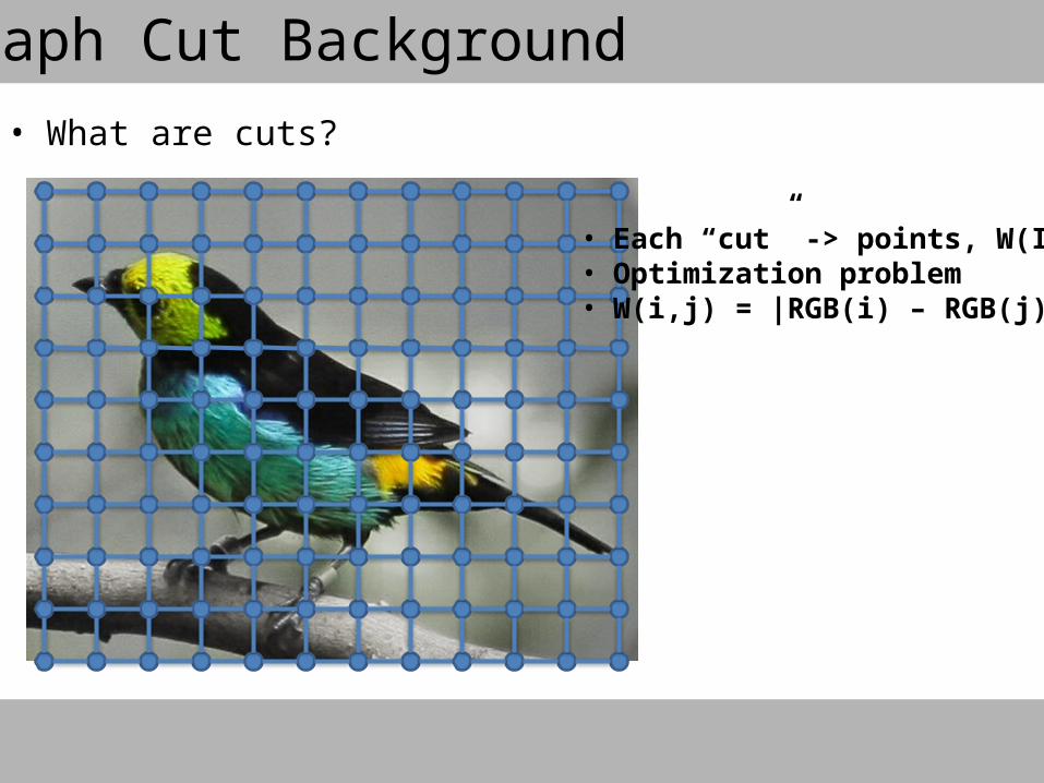
Graph Cut Background• What are cuts?
• Each “cut” -> points, W(I,j)• Optimization problem• W(i,j) = |RGB(i) – RGB(j)|
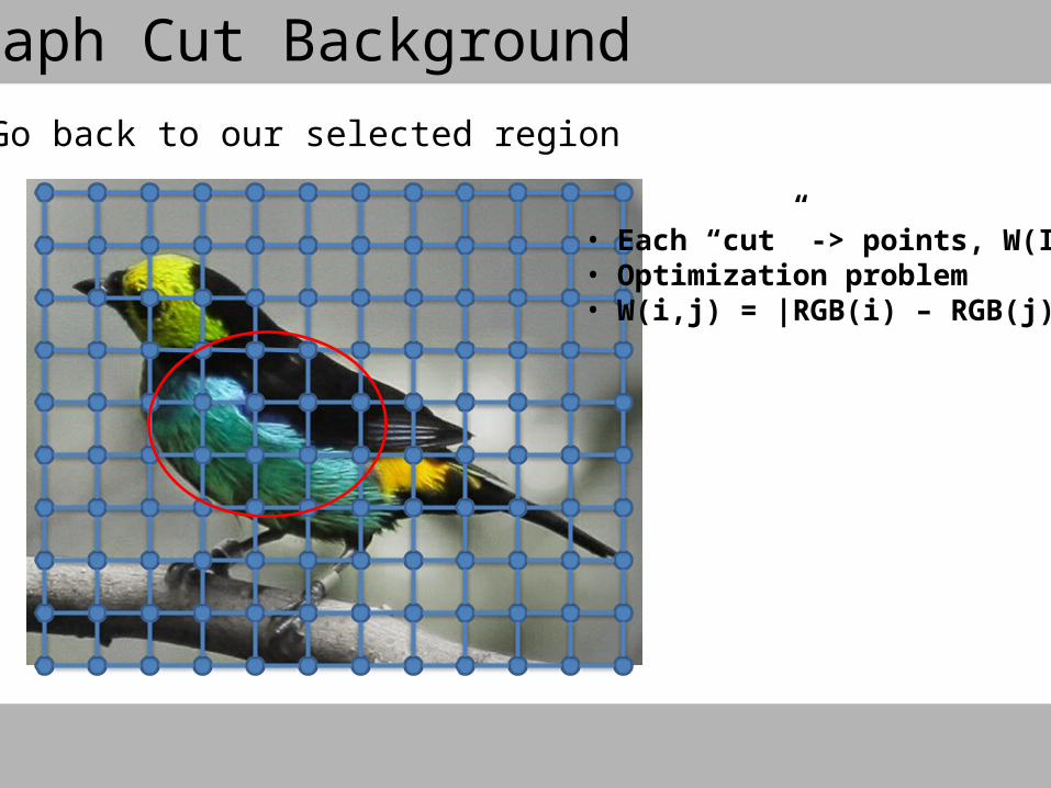
Graph Cut Background• Go back to our selected region
• Each “cut” -> points, W(I,j)• Optimization problem• W(i,j) = |RGB(i) – RGB(j)|
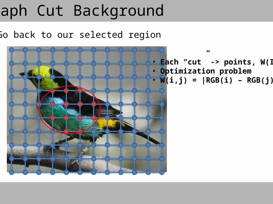
Graph Cut Background• Go back to our selected region
• Each “cut” -> points, W(I,j)• Optimization problem• W(i,j) = |RGB(i) – RGB(j)|

Graph Cut Background• We want highest sum of weights
• Each “cut” -> points, W(I,j)• Optimization problem• W(i,j) = |RGB(i) – RGB(j)|

Graph Cut Background• We want highest sum of weights
• Each “cut” -> points, W(I,j)• Optimization problem• W(i,j) = |RGB(i) – RGB(j)|
These cuts give low pointsW(i,j) = |RGB(i) – RGB(j)|is low
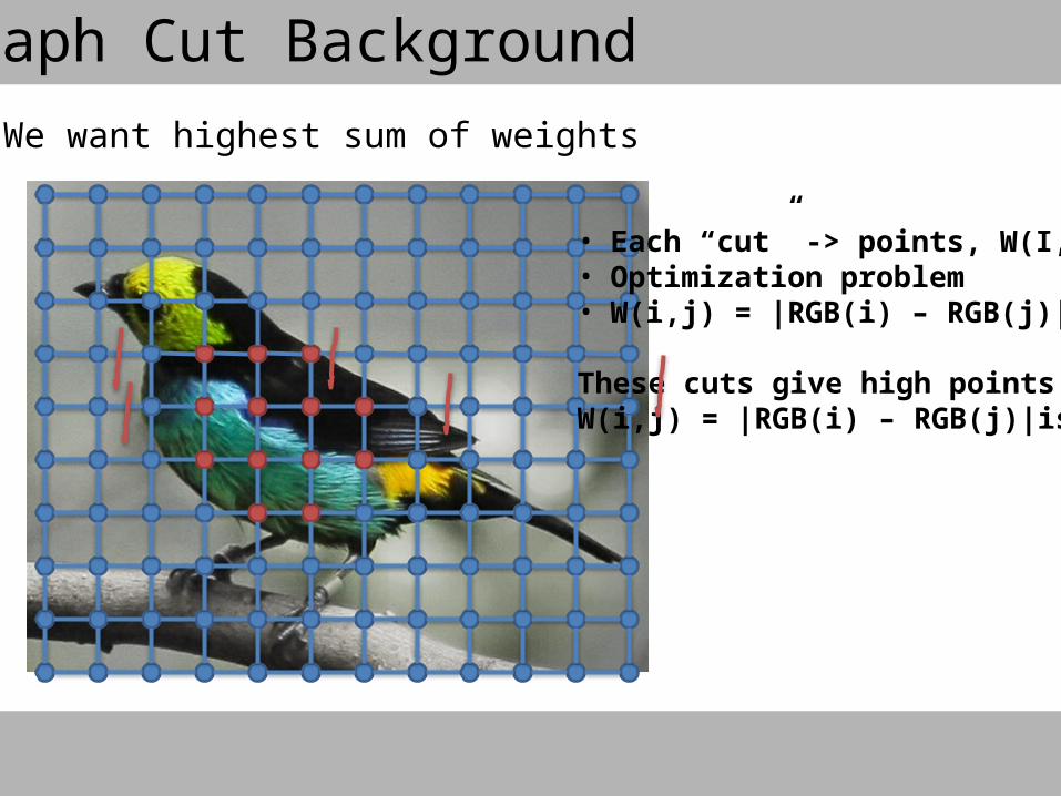
Graph Cut Background• We want highest sum of weights
• Each “cut” -> points, W(I,j)• Optimization problem• W(i,j) = |RGB(i) – RGB(j)|
These cuts give high pointsW(i,j) = |RGB(i) – RGB(j)|is high
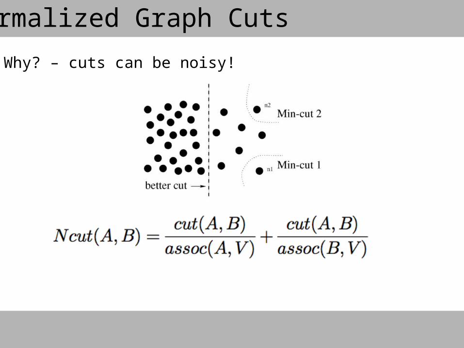
Normalized Graph Cuts
• Why? – cuts can be noisy!
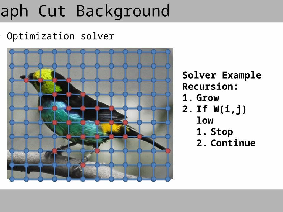
Graph Cut Background• Optimization solver
Solver ExampleRecursion:1. Grow2. If W(i,j) low
1. Stop2. Continue
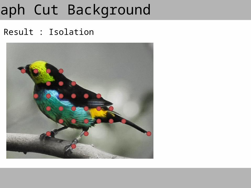
Graph Cut Background• Result : Isolation

Agenda
• History of the problem• Graph cut background• Compute graph cut• Extensions• State of the art• Continued Work
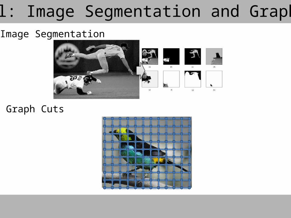
Recall: Image Segmentation and Graph Cuts• Image Segmentation
• Graph Cuts
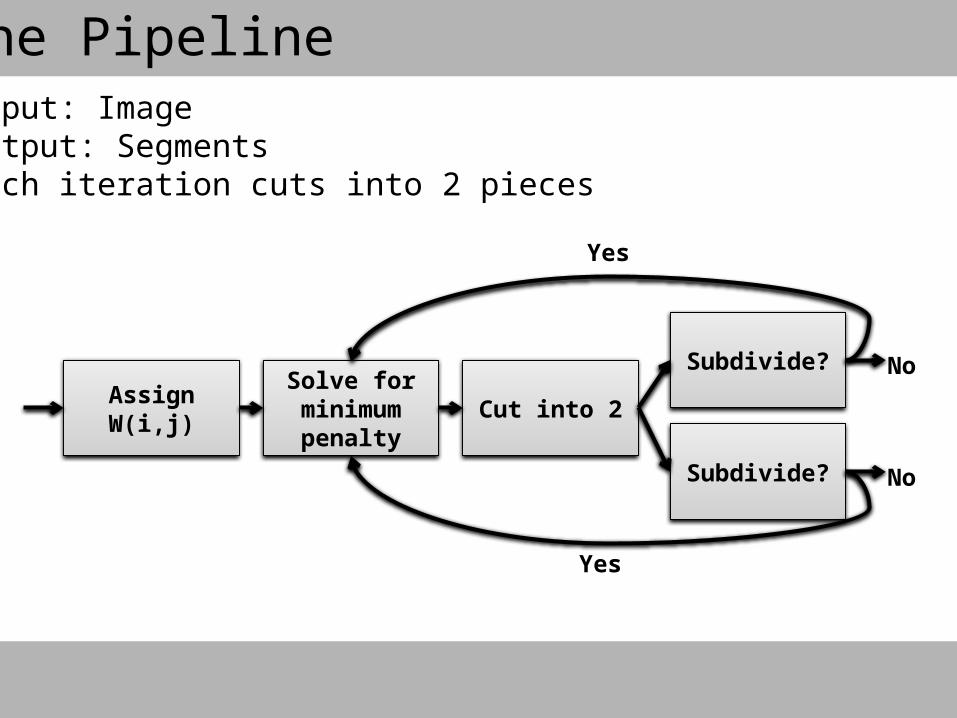
The Pipeline
Assign W(i,j)Solve for minimumpenalty
Cut into 2
Subdivide?
Subdivide?
Yes
Yes
No
No
• Input: Image• Output: Segments• Each iteration cuts into 2 pieces
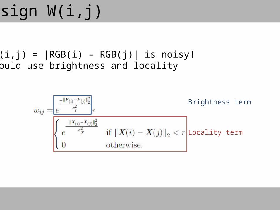
Assign W(i,j)
• W(i,j) = |RGB(i) – RGB(j)| is noisy!• Could use brightness and locality
Brightness term
Locality term

Solve for Minimum Penalty
Summation of edge weights associated with all the points in A
Summation of edge weights associated with the cut
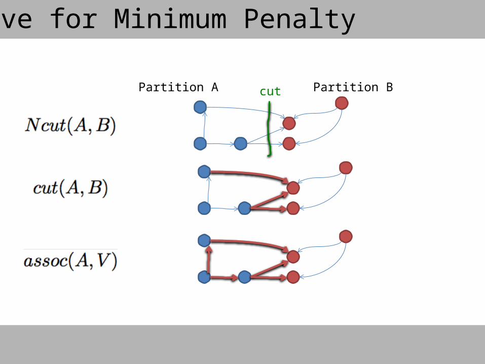
Solve for Minimum Penalty
Partition A Partition Bcut
Solve for Minimum Penalty
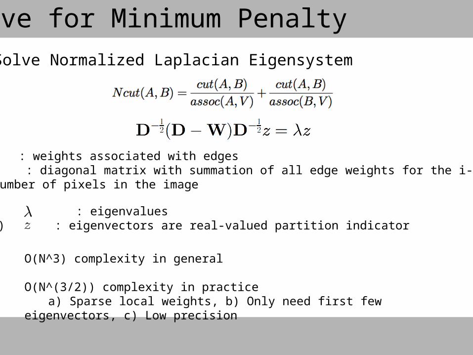
W(N x N) : weights associated with edgesD (N x N) : diagonal matrix with summation of all edge weights for the i-th pixelN : number of pixels in the image
• Solve Normalized Laplacian Eigensystem
O(N^3) complexity in general
O(N^(3/2)) complexity in practicea) Sparse local weights, b) Only need first few eigenvectors, c) Low precision
(N) : eigenvalues (N x N) : eigenvectors are real-valued partition indicator
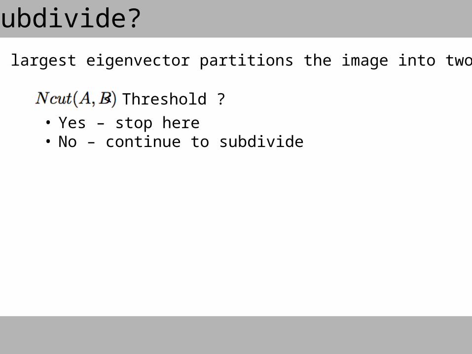
• Second largest eigenvector partitions the image into two regions
•
Subdivide?
< Threshold ?• Yes – stop here• No – continue to subdivide
Agenda
• History of the problem• Graph cut background• Compute graph cut• Extensions• State of the art• Continued Work
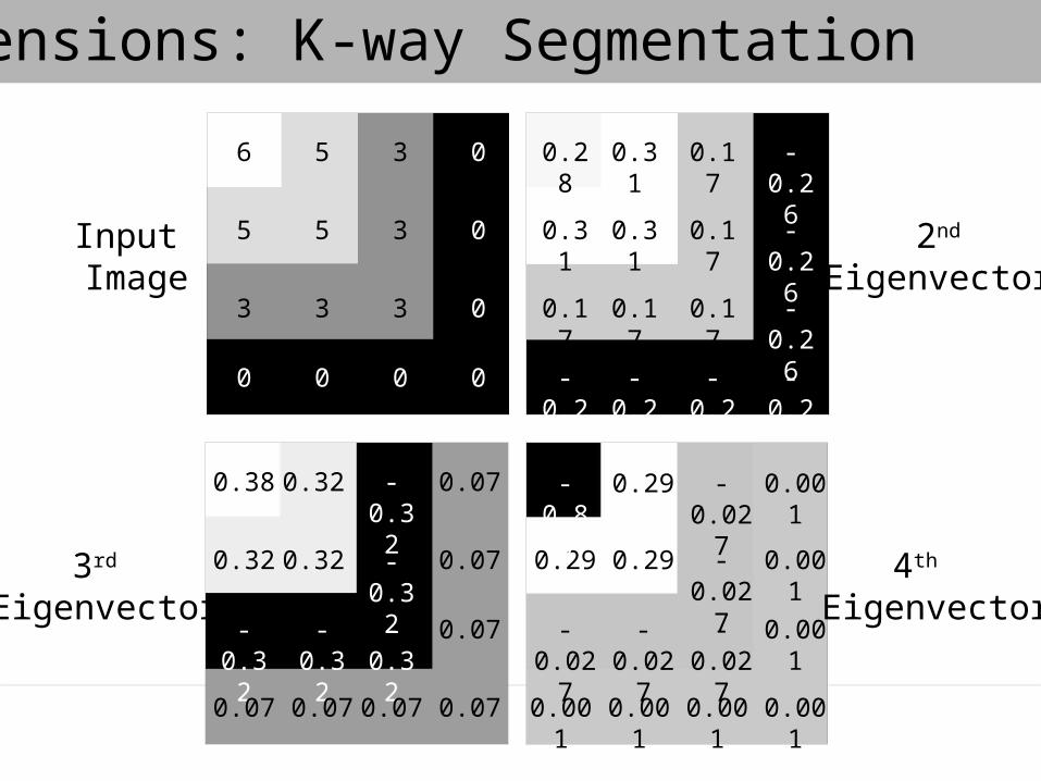
Extensions: K-way Segmentation
6
5 5
5 3
3
333
0
0
0
0000
Input Image
0.28
0.31 0.31
0.31 0.17
0.17
0.170.170.17
-0.26 -0.26 -0.26 -0.26
-0.26
-0.26
-0.26
2nd
Eigenvector
0.001 0.001 0.001 0.001
0.001
0.001
0.001-0.027
-0.027
-0.027
-0.027-0.027
0.29
0.290.29
-0.86
4th Eigenvector
-0.32
-0.32
-0.32-0.32-0.32
0.38
0.32 0.32
0.32 0.07
0.07
0.07
0.070.070.070.07
3rd Eigenvector
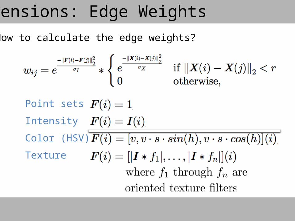
Extensions: Edge Weights• How to calculate the edge weights?
Point sets
Intensity
Color (HSV)
Texture

Agenda
• History of the problem• Graph cut background• Compute graph cut• Extensions• State of the art• Continued Work
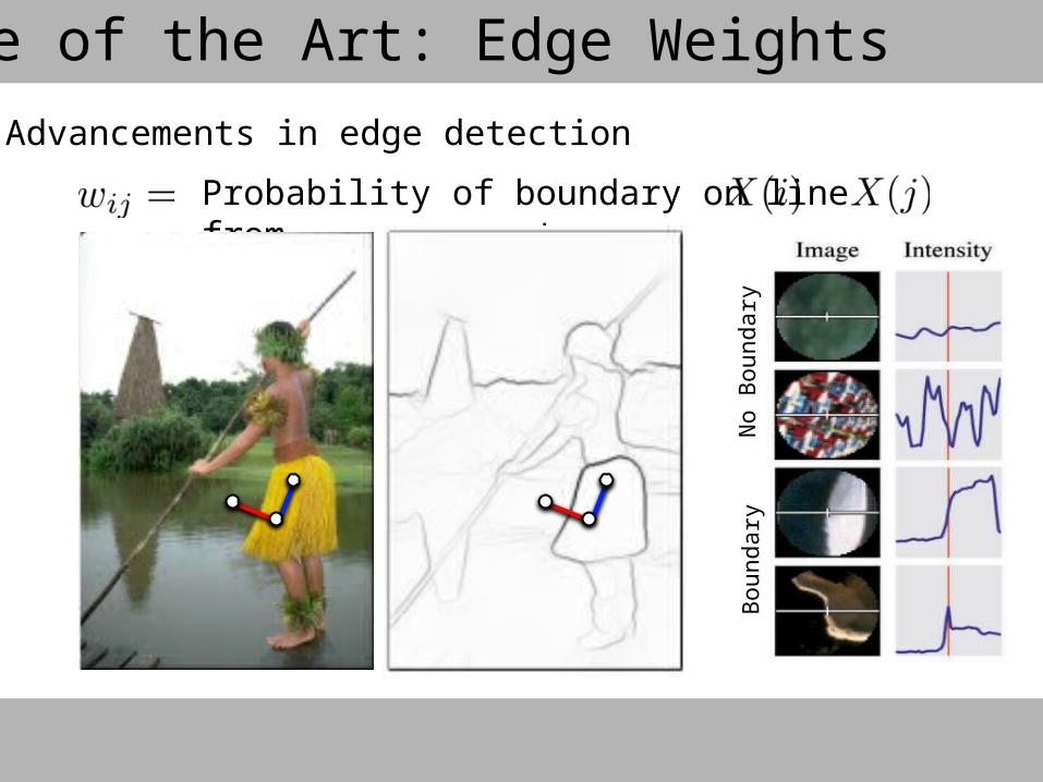
State of the Art: Edge Weights
Probability of boundary on line from to
• Advancements in edge detection
No
Boun
dary
Boun
dary
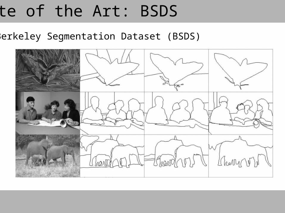
State of the Art: BSDS• Berkeley Segmentation Dataset (BSDS)
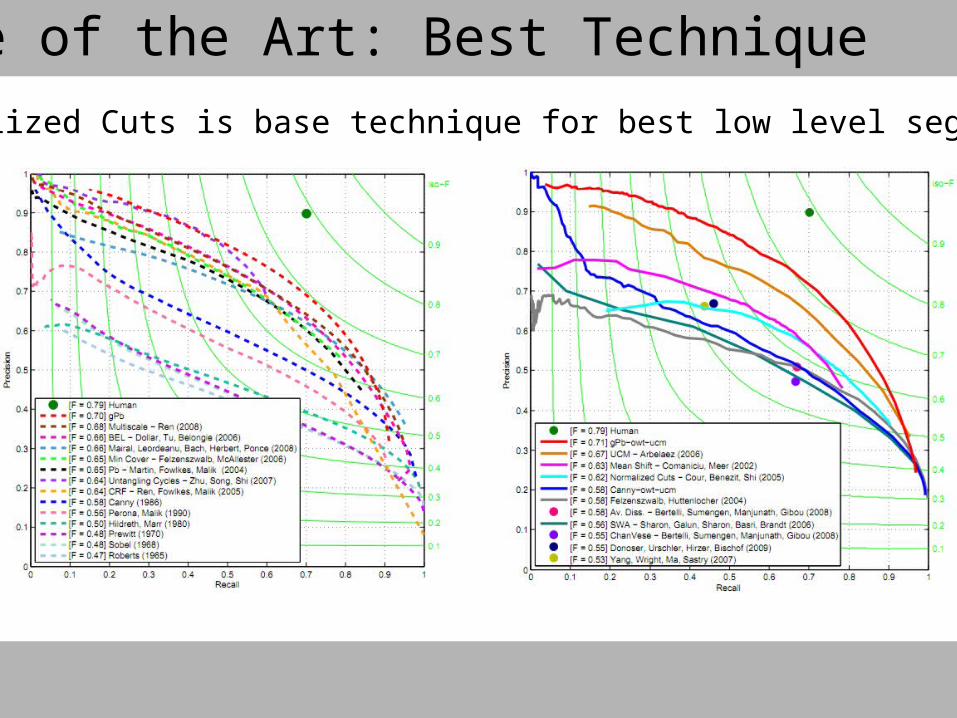
State of the Art: Best Technique• Normalized Cuts is base technique for best low level segmentation

Agenda
• History of the problem• Graph cut background• Compute graph cut• Extensions• State of the art• Continued Work
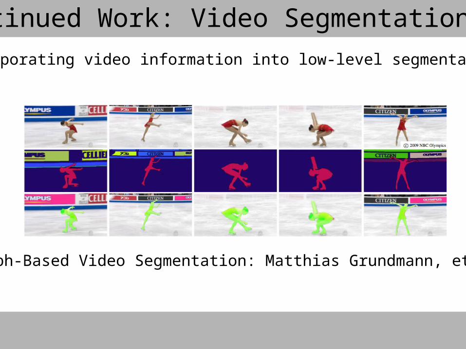
Continued Work: Video Segmentation• Incorporating video information into low-level segmentation
Graph-Based Video Segmentation: Matthias Grundmann, et al

Continued Work: Semantic Segmentation• Incorporating top-down information into low-level segmentation
Interactive Graph Cuts: Yuri Boykov, et al