PREPRINT, ACCEPTED TO SPECIAL ISSUE IEEE TAC, TCAS-I 1

Bistable biological systems: a characterizationthrough local compact input-to-state stability

Madalena Chaves, Thomas Eissing, and Frank Allgower, Member, IEEE

Abstract—Many biological systems have the capacity to operatein two distinct modes, in a stable manner. Typically, the systemcan switch from one stable mode to the other in response to aspecific external input. Mathematically, these bistable systems areusually described by models that exhibit (at least) two distinctstable steady states. On the other hand, to capture biologicalvariability, it seems more natural to associate to each stable modeof operation an appropriate invariant set in the state space ratherthan a single fixed point. A general formulation is proposed in thispaper, which allows freedom in the form of kinetic interactions,and is suitable for establishing conditions on the existence ofone or more disjoint forward-invariant sets for the given system.Stability with respect to each set is studied in terms of a localnotion of input-to-state stability with respect to compact sets.Two well known systems that exhibit bistability are analyzed inthis framework: the lac operon and an apoptosis network. Forthe first example, the question of designing an input that drivesthe system to switch between modes is also considered.

Index Terms—Bistability; Compact input-to-state stability;Biological networks.

I. I NTRODUCTION

B ISTABILITY is a recurrent motif in biology, and thereare many examples of systems which can operate, in

a stable manner, in two very distinct modes. For instance,the well known lac operon in the bacteriaEscherichia coli,a group of genes which are repressed in the presence ofglucose but transcribed in the absence of glucose and presenceof lactose [1], [2]. Another striking example is the phageλvirus, which may exist in either of two states. Under “normal”conditions, this virus can exist in a dormant (lysogentic) state,and survive indefinitely within its host,E. coli. However,under “adverse” conditions, for example after irradiation withultra-violet light [3], the phage can switch to a reproducible(lytic) mode, leading to bacterial lysis (that is, the bacteriaburst). Yet another example is the complex system of cross-talking pathways that regulates the decision of cells to enter theprocess of programmed cell death, also known as apoptosis,as opposed to continuing normal development [4]–[6]. Froma failure in the pro- and anti-apoptotic signaling pathwaysvarious diseases may result, including cancer (where damagedcells that fail to undergo apoptosis, continue to reproduce).

Copyright (c) 2007 IEEE. Personal use of this material is permitted.However, permission to use this material for any other purposes must beobtained from the IEEE by sending an email to pubs-permissions@ieee.org.

M. Chaves is with Project COMORE, INRIA, Centre de recherche deSophia Antipolis, 2004 Route des Lucioles, BP 93, 06902 Sophia Antipolis,France. T. Eissing and F. Allgower are with the Institute for Systems Theoryand Automatic Control, University of Stuttgart, Pfaffenwaldring 9, 70550Stuttgart, Germany. Emails: M. Chaves, mchaves@sophia.inria.fr (correspond-ing author, tel: +33 492 38 50 49, fax: +33 492 38 78 58); T. Eissing,eissing@ist.uni-stuttgart.de; F. Allgower, allgower@ist.uni-stuttgart.de.

Bistable behavior has been experimentally detected at thesingle cell level (for example, thelac operon inE. Coli [2] andthe cell cycle oscillator inXenopus laevis[7]). These beautifulexperiments show that each individual cell can indeed onlyexist in one of two distinct states, and upon stimulation with anappropriate input, a clear jump-like transition is observed, fromone state to another. To understand how each bistable systemworks, many mathematical models have been proposed, but acommon feature is the existence of an appropriate positivefeedback loop (see, for instance, [6], [8] for analysis of acaspase cascade at the heart of apoptosis). A general methodfor multistability in a large class of biological systems isprovided in [9], using the concept of monotone systems. Onthe other hand, at the population level, a graded response toincreasing stimuli is typically observed [2], [10]. This meansthat each cell has its own “threshold”, its own particular pointwhere it will jump from one steady state to the other. Sincethis threshold varies from cell to cell, a population experimentshould reflect the fraction of cells in a given steady state foreach given stimulus concentration.

This introduces a fundamental issue of concern when mod-eling and studying biological systems: the inherent variabil-ity encountered among different “realizations” of the samesystem. Various modeling techniques have been suggestedand used to deal with the problem of variability, and obtainever more realistic descriptions of the biological systems.Just to cite some examples, among many others: stochasticmodels [11], [12], discrete/logical models which provide morequalitative descriptions [13]–[16], and more recently hybridmodels [17], and in particular piecewise linear models [18]–[22]. The system under study, its complexity, and the knowl-edge and experimental data available, often determine themost suitable method for modeling a given system. In thecase of genetic regulatory networks, although exact formsfor the interactions are often not known, the presence (orexpression) of a given protein or mRNA is typically due tothe appropriate combination of presence or absence of anothergroup of species [23].

An alternative approach is proposed here, which providesan intuitive bridge between continuous models and the classof piecewise linear hybrid models. This approach is speciallyattractive for the type of systems whose interactions can bedescribed as combinations of “activation” and “inhibition”functions. These functions will be generally formulated in thesense that, instead of a specific mathematical formula, theyare bounded within appropriate “tubes”. In this context, onemay expect a mathematical model for a bistable biologicalsystem to exhibit two distinct, disjoint, forward-invariant sets

PREPRINT, ACCEPTED TO SPECIAL ISSUE IEEE TAC, TCAS-I 2

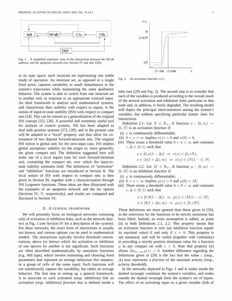
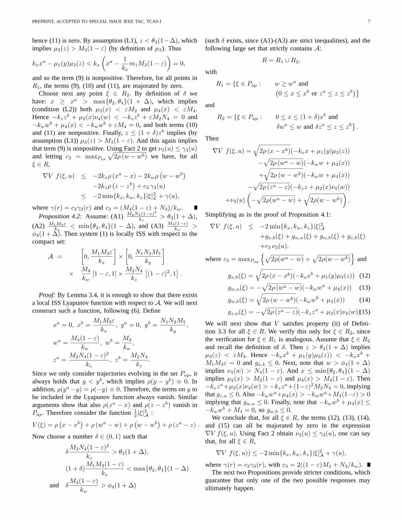
Fig. 1. A simplified schematic view of the interactions between the NFκBpathway and the apoptosis network (see Section IV and also [29]).

in its state space: each invariant set representing one stablemode of operation. An invariant set, as opposed to a singlefixed point, captures variability or small disturbances in thesystem’s trajectories while maintaining the same qualitativebehavior. The system is able to switch from one invariant setto another only in response to an appropriate external input.An ideal framework to analyze such mathematical systems,and characterize their stability with respect to inputs, is thenotion of input-to-state stability (ISS) with respect to compactsets [24]. This can be viewed as a generalization of the originalISS concept [25], [26]. A powerful and extremely useful toolfor analysis of control systems, ISS has been adapted todeal with positive systems [27], [28], and in the present casewill be adapted to a “local” property, and thus allow for co-existence of two disjoint forward-invariant sets. The originalISS notion is global and, for the zero-input case, ISS impliesglobal asymptotic stability (to the origin or, more generally,the given compact set). The definition suggested here willmake use of a local region (one for each forward-invariantset), containing the compact set, over which the input-to-state stability estimates hold. The definitions of “activation”and “inhibition” functions are introduced in Section II. Thelocal notion of ISS with respect to compact sets is thengiven in Section III, together with a characterization throughISS Lyapunov functions. These ideas are then illustrated withthe examples of an apoptosis network and thelac operon(Sections IV, V, respectively), and results are compared anddiscussed in Section VI.

II. A GENERAL FRAMEWORK

We will presently focus on biological networks consistingonly of activation or inhibition links, such as the network depi-tect in Fig. 1 (see Section IV for a description of the system).For these networks, the exact form of interactions is usuallynot known, and various options can be used in mathematicalmodels. The interactions typically involve threshold concen-trations, above (or below) which the activation or inhibitionof one species by another is not significant. Such functionsare often described mathematically by saturation functions(e.g. Hill type), which involve estimating and choosing fixedparameters that represent an average behaviour (for instance,in a group of cells of the same type). Such functions willnot satisfactorily capture the variability, but rather an averagebehavior. The first step in setting up a general framework,is to associate to each activation (resp. inhibition) link anactivation (resp. inhibition) functionthat is defined inside a

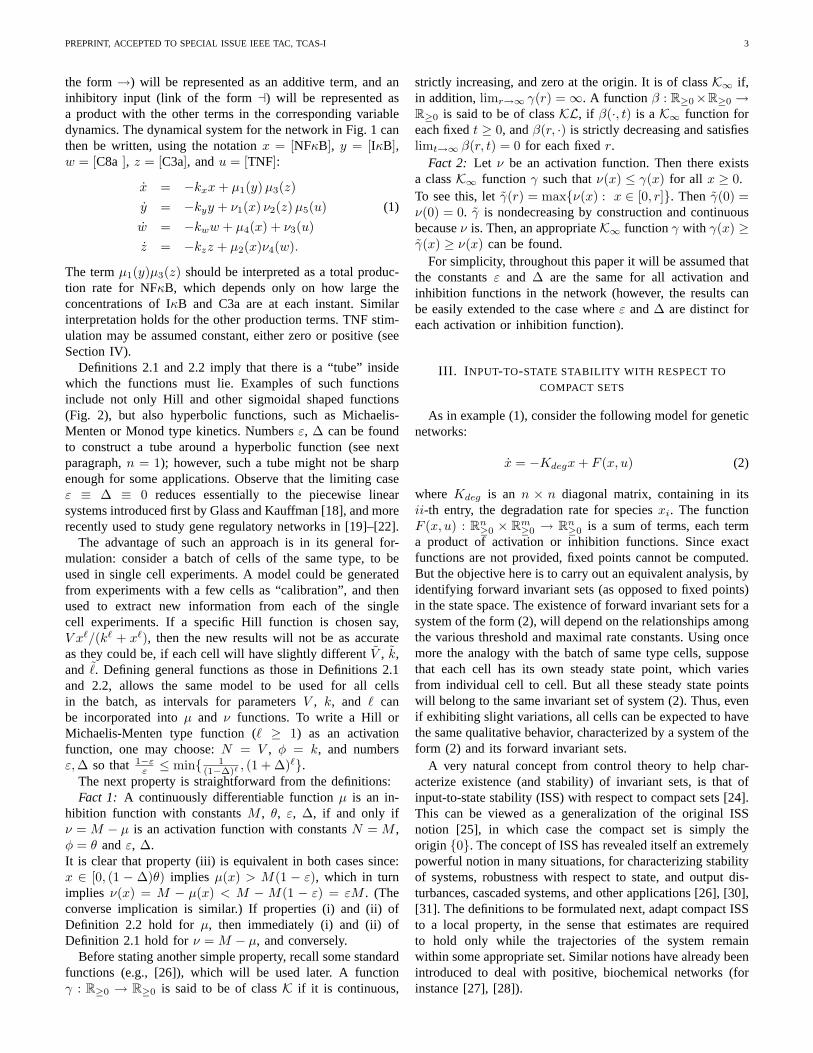
Fig. 2. An activation functionν(x).

tube (see [29] and Fig. 2). The second step is to consider thateach of the variables is produced according to the overall resultof the several activation and inhibition links particular to thatnode and, in addition, is freely degraded. The resulting modelwill depict the principal interconnetions among the system’svariables, but without specifying particular kinetic laws forinteractions.

Definition 2.1: Let N ∈ R+. A function ν : [0,∞) →[0, N ] is anactivation functionif:(i) ν is continuously differentiable;

(ii) 0 < x < ∞ implies ν(x) > 0 andν(0) = 0;(iii) There exists a threshold value0 < φ < ∞ and constants

ε, ∆ ∈ (0, 1) such that

x ∈ [0, φ(1−∆)) ⇒ ν(x) ∈ [0, εN),x ∈ (φ(1 + ∆),∞) ⇒ ν(x) ∈ (N(1− ε), N ].

Definition 2.2: Let M ∈ R+. A function µ : [0,∞) →[0,M ] is an inhibition function if:(i) µ is continuously differentiable;

(ii) 0 < x < ∞ implies µ(x) > 0 andµ(0) = M ;(iii) There exists a threshold value0 < θ < ∞ and constants

ε, ∆ ∈ (0, 1) such that

x ∈ [0, θ(1−∆)) ⇒ µ(x) ∈ (M(1− ε),M ],x ∈ (θ(1 + ∆),∞) ⇒ µ(x) ∈ [0, εM).

These definitions are more general than those given in [29],as the restriction for the functions to be strictly monotone hasbeen lifted. Instead, an extra assumption is added, as point(ii) in both Definitions 2.1, 2.2. This property means thatan activation function is zero (an inhibition function equalsits maximal value) if and only ifx = 0. This property isnot unnatural, and will be useful (together with continuity)in providing a strictly positive minimum value for a functionµ in any compact set withx > 0. Note that property (ii)allows limx→∞ µ(x) = 0. Another difference regarding thedefinitions given in [29] is the fact that the valueε (resp.,∆) now represents afraction of the maximal activity (resp.,activity threshold).

In the networks depicted in Figs. 1 and 4, nodes inside thedashed rectangle constitute the system’s variables, and nodesoutside the dashed rectangle form the system’s set of inputs.The effect of an activating input on a given variable (link of

PREPRINT, ACCEPTED TO SPECIAL ISSUE IEEE TAC, TCAS-I 3

the form→) will be represented as an additive term, and aninhibitory input (link of the forma) will be represented asa product with the other terms in the corresponding variabledynamics. The dynamical system for the network in Fig. 1 canthen be written, using the notationx = [NFκB], y = [IκB],w = [C8a ], z = [C3a], andu = [TNF]:

x = −kxx + µ1(y) µ3(z)y = −kyy + ν1(x) ν2(z) µ5(u) (1)

w = −kww + µ4(x) + ν3(u)z = −kzz + µ2(x)ν4(w).

The termµ1(y)µ3(z) should be interpreted as a total produc-tion rate for NFκB, which depends only on how large theconcentrations of IκB and C3a are at each instant. Similarinterpretation holds for the other production terms. TNF stim-ulation may be assumed constant, either zero or positive (seeSection IV).

Definitions 2.1 and 2.2 imply that there is a “tube” insidewhich the functions must lie. Examples of such functionsinclude not only Hill and other sigmoidal shaped functions(Fig. 2), but also hyperbolic functions, such as Michaelis-Menten or Monod type kinetics. Numbersε, ∆ can be foundto construct a tube around a hyperbolic function (see nextparagraph,n = 1); however, such a tube might not be sharpenough for some applications. Observe that the limiting caseε ≡ ∆ ≡ 0 reduces essentially to the piecewise linearsystems introduced first by Glass and Kauffman [18], and morerecently used to study gene regulatory networks in [19]–[22].

The advantage of such an approach is in its general for-mulation: consider a batch of cells of the same type, to beused in single cell experiments. A model could be generatedfrom experiments with a few cells as “calibration”, and thenused to extract new information from each of the singlecell experiments. If a specific Hill function is chosen say,V x`/(k` + x`), then the new results will not be as accurateas they could be, if each cell will have slightly differentV , k,and ˜. Defining general functions as those in Definitions 2.1and 2.2, allows the same model to be used for all cellsin the batch, as intervals for parametersV , k, and ` canbe incorporated intoµ and ν functions. To write a Hill orMichaelis-Menten type function (` ≥ 1) as an activationfunction, one may choose:N = V , φ = k, and numbersε, ∆ so that 1−ε

ε ≤ min{ 1(1−∆)` , (1 + ∆)`}.

The next property is straightforward from the definitions:Fact 1: A continuously differentiable functionµ is an in-

hibition function with constantsM , θ, ε, ∆, if and only ifν = M − µ is an activation function with constantsN = M ,φ = θ andε, ∆.It is clear that property (iii) is equivalent in both cases since:x ∈ [0, (1 − ∆)θ) implies µ(x) > M(1 − ε), which in turnimplies ν(x) = M − µ(x) < M − M(1 − ε) = εM . (Theconverse implication is similar.) If properties (i) and (ii) ofDefinition 2.2 hold forµ, then immediately (i) and (ii) ofDefinition 2.1 hold forν = M − µ, and conversely.

Before stating another simple property, recall some standardfunctions (e.g., [26]), which will be used later. A functionγ : R≥0 → R≥0 is said to be of classK if it is continuous,

strictly increasing, and zero at the origin. It is of classK∞ if,in addition,limr→∞ γ(r) = ∞. A function β : R≥0×R≥0 →R≥0 is said to be of classKL, if β(·, t) is aK∞ function foreach fixedt ≥ 0, andβ(r, ·) is strictly decreasing and satisfieslimt→∞ β(r, t) = 0 for each fixedr.

Fact 2: Let ν be an activation function. Then there existsa classK∞ function γ such thatν(x) ≤ γ(x) for all x ≥ 0.To see this, letγ(r) = max{ν(x) : x ∈ [0, r]}. Then γ(0) =ν(0) = 0. γ is nondecreasing by construction and continuousbecauseν is. Then, an appropriateK∞ functionγ with γ(x) ≥γ(x) ≥ ν(x) can be found.

For simplicity, throughout this paper it will be assumed thatthe constantsε and ∆ are the same for all activation andinhibition functions in the network (however, the results canbe easily extended to the case whereε and∆ are distinct foreach activation or inhibition function).

III. I NPUT-TO-STATE STABILITY WITH RESPECT TO

COMPACT SETS

As in example (1), consider the following model for geneticnetworks:

x = −Kdegx + F (x, u) (2)

where Kdeg is an n × n diagonal matrix, containing in itsii-th entry, the degradation rate for speciesxi. The functionF (x, u) : Rn

≥0 × Rm≥0 → Rn

≥0 is a sum of terms, each terma product of activation or inhibition functions. Since exactfunctions are not provided, fixed points cannot be computed.But the objective here is to carry out an equivalent analysis, byidentifying forward invariant sets (as opposed to fixed points)in the state space. The existence of forward invariant sets for asystem of the form (2), will depend on the relationships amongthe various threshold and maximal rate constants. Using oncemore the analogy with the batch of same type cells, supposethat each cell has its own steady state point, which variesfrom individual cell to cell. But all these steady state pointswill belong to the same invariant set of system (2). Thus, evenif exhibiting slight variations, all cells can be expected to havethe same qualitative behavior, characterized by a system of theform (2) and its forward invariant sets.

A very natural concept from control theory to help char-acterize existence (and stability) of invariant sets, is that ofinput-to-state stability (ISS) with respect to compact sets [24].This can be viewed as a generalization of the original ISSnotion [25], in which case the compact set is simply theorigin {0}. The concept of ISS has revealed itself an extremelypowerful notion in many situations, for characterizing stabilityof systems, robustness with respect to state, and output dis-turbances, cascaded systems, and other applications [26], [30],[31]. The definitions to be formulated next, adapt compact ISSto a local property, in the sense that estimates are requiredto hold only while the trajectories of the system remainwithin some appropriate set. Similar notions have already beenintroduced to deal with positive, biochemical networks (forinstance [27], [28]).

PREPRINT, ACCEPTED TO SPECIAL ISSUE IEEE TAC, TCAS-I 4

A. Local notions of compact ISS

In the definitions to follow next, for simplicity consider asystem with inputsx = f(x, u), evolving in a setX ⊂ Rn

≥0,wheref(·, u) is continuously differentiable for each fixedu,and define aninput to be a locally Lipschitz functionw :R≥0 → Rm

≥0. Let |u| denote the usual Euclidean norm formatrices and define also:

‖u‖ = ess. sup .{|u(t)| : t ∈ [0,+∞)}.

In the next definition, let0 < Tmax ≤ ∞ and assume thatJx0,w = [0, Tmax) is the interval where the maximal solutionof a systemx = f(x, u), for an initial condtionx0 and inputw, is defined.

Definition 3.1: A setP is forward-invariant for the systemx = f(x, u) if, for each initial statex(0) = x0 ∈ P , and eachinput w(·), the corresponding maximal solutionx(t, x0, w),which is defined on an intervalJx0,w = [0, Tmax), satisfiesx(t, x0, w) ∈ P for all t ∈ Jx0,w. The system isP -forwardcomplete ifP is a forward invariant set for the system and, inaddition,Jx0,w = [0,∞), for eachx(0) = x0 ∈ P and eachinput w(·).

Following [24], letQ be a nonempty compact set ofRn≥0.

Then define the usual point-to-set distance:

|x|Q = inf{|x− q|, q ∈ Q}.

In our examples, as in many biological systems, the setX is aproduct of intervalsΠn

i=1 [0, ai], for finiteai, i = 1, . . . , n. Thecompact sets to be considered will often touch the boundaryof X , for instanceQ = {x ∈ X : 0 ≤ x1 ≤ εa1}, with0 < ε < 1. In this context, we will still say thatQ is containedin the interior ofX . More generally we define:

intXR := {x ∈ R : x ∈ int R or x ∈ ∂R ∩ ∂X} . (3)

Definition 3.2: Assume that the systemx = f(x, u), is X -forward complete. Then the system islocally input-to-statestable with respect to a compact setQ if there exists a setR ⊂ X with Q ⊂ intXR, and functionsβ = βR of classKLandϕ = ϕR of classK∞ such that, for every initial conditionx0 ∈ R and each inputw(·) :

|x(t, x0, w)|Q ≤ β(|x0|Q, t) + ϕ(‖w‖), (4)

for all t ≥ 0 such thatx(s) ∈ R for all s ∈ [0, t].If R = X then the system isglobally input-to-state stable

with respect to the compact setQ.Definition 3.3: A continuously differentiable functionV :

Rn≥0 → R≥0 is a local ISS Lyapunov function with respect to

a compact setQ for the systemx = f(x, u), if:

(i) there exist functionsν1, ν2 ∈ K∞, so that

ν1(|x|Q) ≤ V (x) ≤ ν2(|x|Q)

for all x ∈ Rn≥0.

(ii) there exists a setR ⊂ X with Q ⊂ intXR, and functionsα = αR, γ = γR ∈ K∞ such that

∇V (x) f(x, u) ≤ −α(|x|Q) + γ(|u|)

for everyx ∈ R.

If R = X , then the functionV is a global ISS Lyapunovfunction with respect to the compact setQ for the system.

The local condition means that the ISS estimate will remainvalid as long as the trajectory evolves within the given setR.As in the case of the original definition of an ISS system,the existence of an ISS-Lyapunov function with respect toa compact setQ implies that the system is input-to-statestable with respect to that compact setQ. The proof of thisresult is very similar to the original one, and follows closelythe argument given in [26], hence we do not include it (seealso [27]).

Lemma 3.4:Consider anRn≥0- forward complete system

x = f(x, u). Suppose thatV is a local (resp., global) ISSLyapunov function with respect to the compact setQ ⊂ Rn

≥0.Then, the system is locally (resp., globally) input-to-statestable with respect to the compact setQ. �

If the system is globally ISS with respect to a compact setQ, then this set is said to be0-invariant for the system, thatis the solution of

x = f(x, 0), x(0) = x0 ∈ Q

remains inQ for all t ≥ 0, that is,x(t, x0, 0) ∈ Q wheneverx0 ∈ Q. Furthermore, if a system is globally ISS with respectto Q, then in the caseu(t) ≡ 0, the trajectories globallyasymptotically converge toQ. It is not difficult to check thatthe definition of local compact ISS also implies 0-invarianceof the setQ. One needs only to verify that, whenu(t) ≡ 0 andx0 ∈ Q, the trajectories do not leave the setR. To see this,simply note that (4) together withu(t) ≡ 0 and x0 ∈ Q, infact imply |x(t, x0, w)|Q ≤ 0 for all times. Using Lemma 3.4the following result holds.

Lemma 3.5:If there exists a local ISS Lyapunov functionwith respect to the compact setQ for the systemx = f(x, u),thenQ is a 0-invariant set for the system.

The definition in local terms is useful when there exist two(or more) disjoint 0-invariant sets for the system (as is thecase with bistable systems). In this case, global asymptoticstability to either set (in the caseu ≡ 0) clearly does not makesense, but it is still meaningful to characterize the regions ofstate space (the setR) from where it is possible to eventuallyconverge to one of the sets. In addition, if starting inside oneof the invariant sets, local ISS with respect to a compact setquantifies the magnitude of disturbances allowed before thesystem leaves that set.

B. ISS Lyapunov functions with respect to cubes

For systems of the form (2) and for compact sets whichare products of closed intervals, it is possible to use “piece-wise” quadratic functions to systematically construct an ISSLyapunov function with respect to a given cube. Define thescalar function:

ρ(r) ={

12r2, r ≥ 00, r < 0 .

This function is continuously differentiable and satisfies:

rdρ

dr= r

√2ρ(r) = 2 ρ(r). (5)

PREPRINT, ACCEPTED TO SPECIAL ISSUE IEEE TAC, TCAS-I 5

Now consider a set of the form

Q = [xa1 , xb

1]× · · · × [xan, xb

n].

Then our candidate Lyapunov function will be:

V (x) =12|x|2Q =

n∑i=1

ρ(xai − xi) + ρ(xi − xb

i ). (6)

This is the squared point-to-set distance to a cube-shapedcompact set, and hence one may setν1 = ν2 = V (x) = 1

2 |x|2Q.

Using thisV , and noticing that the functionF (x, u) in (2)is bounded (as a finite sum of products of activation andinhibition functions), it is easy to prove the following result.

Lemma 3.6:DefineFi = maxx,u Fi(x, u) and consider theset

P =[0,

F1

k1

]× · · · ×

[0,

Fn

kn

]. (7)

Then system (2) isP -forward complete.Proof: The function−Kdegx + F (x, u) is continuously dif-ferentiable onRn

≥0 for each fixedu, and locally integrable onRm≥0 for each fixedx ∈ Rn

≥0. For each continuous inputw, andinitial condition x0 ∈ P , let x(t, x0, w) denote the maximalsolution of the initial value problemx(t) = −Kdegx(t) +F (x(t), w(t)), x(0) = x0, and suppose it is defined on aninterval [0, Tmax). Consider now the distance function

V (x) =12|x|2P =

n∑i=1

ρ

(xi −

Fi

ki

),

since the system is defined only for nonnegative coordinates.Then (writingxi = (xi − F /ki) + F /ki)

∇V f(x, u) =n∑

i=1

√2ρ

(xi −

Fi

ki

) (−ki(xi −

Fi

ki))

+n∑

i=1

√2ρ

(xi −

Fi

ki

)(−Fi + Fi(x, u))

≤n∑

i=1

−ki2 ρ

(xi −

Fi

ki

)≤ −2 min

iki |x|2P

because (by definition ofF ) −Fi + Fi(x, u) ≤ 0 for all iand allx, u. It is clear thatV (x(t, x0, w)) is a nonincreasingfunction so, for allt > 0,

|x(t, x0, w)|2P ≤ |x0|2P ,

implying that the trajectory remains bounded for all times,and henceTmax = ∞. By a comparison principle, it alsoholds that:V (x(t, x0, w)) ≤ exp(−c|x(t, x0, w)|2P ) (wherec = 2 mini ki). Therefore, the trajectories of system (2) areasymptotically convergent to the compact setP . Finally, ifthe initial condition isx0 ∈ P , then|x(t, x0, w)|2P ≡ 0 for allt, meaning that system (2) is indeedP -forward complete.

From now on, without loss of generality, we will consideronly trajectories of (2) evolving inP . For system (1) this set

becomes:

Pap =[0,

M1M3

kx

]×

[0,

N1N2M5

ky

]×

[0,

M4 + N3

kw

]×

[0,

M2N4

kz

].

IV. L IFE AND DEATH DECISION IN AN APOPTOSIS

NETWORK

The apoptosis network is responsible for programmed celldeath in response to certain stimuli. Apoptosis enables theorganisms to eliminate unwanted cells and thus prevent, forinstance, replication of damaged cells (see for example [4]).Cancer, as well as other diseases, may develop if the apoptosisnetwork fails to respond in an appropriate manner. At the heartof the apoptosis network is a family of proteins (caspases, eachexisting in a pro-form and an active form), which are activatedin a cascade (for more references see [4] and also [6]). Caspase3 (C3) is a prominent downstream member of this cascade,and it is responsible for the cleavage (and destruction) ofvarious and critical proteins in the cell: thus high abundance ofactive C3 (C3a) typically leads to cell death. Other pathwaysinteract with the apoptosis network, in particular the wellknown Nuclear FactorκB (NFκB) pathway [4]. NFκB isa transcription factor responsible for transcription of variousgenes, including one for its own inhibitor (IκB), and anotherfor an inhibitor of C3a (IAP). Thus, the presence of NFκB (or,more precisely, its transcription products) typically promotessurvival of the cell. While the NFκB pathway can be generallyconsidered an anti-apoptotic pathway, it is often activated inparallel with the pro-apoptotic caspase cascade. A commonsignal is stimulation of extrinsic death receptors, for example,Tumor Necrosis Factor (TNF) activating its receptor TNFR1.TNFR1 activation leads to deactivation of IκB. On the otherhand, TNF activates caspase 8, which in turn activates caspase3, and NFκB also functions as an inhibitor of this step (throughthe activity of FLIP, an inhibitor of caspase 8 activation andIAPs, inhibitors of C3a) [4]. The interaction among pro-and anti-apoptotic modules will influence and fine tune thecellular decision to survive or undergo apoptosis [32]. Thus, inmodel (1) a “living” response corresponds to low concentrationof C3a (and high concentration of NFκB), and conversely an“apoptotic” response corresponds to high concentration of C3a(and low concentration of NFκB).

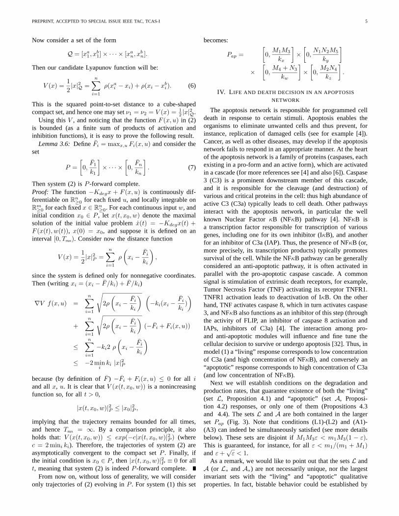
Next we will establish conditions on the degradation andproduction rates, that guarantee existence of both the “living”(set L, Proposition 4.1) and “apoptotic” (setA, Proposi-tion 4.2) responses, or only one of them (Propositions 4.3and 4.4). The setsL andA are both contained in the largerset Pap (Fig. 3). Note that conditions (L1)-(L2) and (A1)-(A3) can indeed be simultaneously satisfied (see more detailsbelow). These sets are disjoint ifM1M3ε < m1M3(1 − ε).This is guaranteed, for instance, for allε < m1/(m1 + M1)andε +

√ε < 1.

As a remark, we would like to point out that the setsL andA (or L∗ andA∗) are not necessarily unique, nor the largestinvariant sets with the “living” and “apoptotic” qualitativeproperties. In fact, bistable behavior could be established by

PREPRINT, ACCEPTED TO SPECIAL ISSUE IEEE TAC, TCAS-I 6

Fig. 3. The “living” (L) and “apoptosis” (A) 0-invariant sets, projected intothe planex = [NFκB], z = [C3a]. Also shown (shaded) is the local setRfor the “living set”.

finding any other suitable pair of disjoint 0-invariant compactsets, sayL and A, with the properties “highx / low w”and “low x / high w”, under different assumptions on theparameters of the network. The goal here is to show thatthe network has the capacity for bistability, by identifyingconditions for which at least one pair of setsL,A co-exist. Or,alternatively, conditions on the parameters for which bistabilityis lost and only one of the sets is invariant.

Recall that system (1) is Pap-forward complete(Lemma 3.6). Define

m1 = min{

µ1(y) : y ∈[0,

N1N2M5

ky

]}, (8)

which is a stricly positive constant, becauseµ1 is continuous,and by property (ii) of Definition 2.2. To simplify notation, letξ = (x, y, w, z)′, and letξ = f(ξ, u) denote system (1).

Proposition 4.1:Assume that (L1)εM2N4kz

< θ3(1 − ∆),and (L2) m1M3(1−ε)

kx> max{θ2, θ4}(1+∆). Then system (1)

is locally ISS with respect to the compact set:

L =[m1M3(1− ε)

kx,M1M3

kx

]×

[0,

N1N2M5

ky

]×

[0,

εM4

kw

]×

[0,

εM2N4

kz

].

Proof: By Lemma 3.4, it is enough to show that there existsa local ISS Lyapunov function with respect toL. We will nextconstruct such a function, following (6). Set

xa =m1M3(1− ε)

kx, xb =

M1M3

kx,

ya = 0, yb =N1N2M5

ky,

wa = 0, wb =εM4

kw, za = 0, zb =

εM2N4

kz.

Since we only consider trajectories evolving in the setPap, italways holds thaty < yb, which impliesρ(y − yb) ≡ 0. Inaddition,ρ(ya−y) = ρ(−y) ≡ 0. Therefore, the terms ony tobe included in the Lyapunov function always vanish. Similar

arguments show that alsoρ(x−xb), ρ(wa−w) andρ(za−z)identically vanish in the state spacePap. Therefore considerthe function:

V (ξ) =12|ξ|2L = ρ (xa − x) + ρ

(w − wb

)+ ρ

(z − zb

).

Now choose a numberδ ∈ (0, 1) such that

(1 + δ)εM2N4

kz< θ3(1−∆) and

δm1M3(1− ε)

kx> max{θ2, θ4}(1 + ∆)

(such δ exists, since (L1)-(L2) are strict inequalities), andconsider the following set which containsL in its interior:

R = R1 ∪R2,

R1 ={ξ ∈ Pap : w ≤ wb and (xa ≤ x ≤ xb or z ≤ zb)

}R2 =

{ξ ∈ Pap : δxa ≤ x ≤ xb andz ≤ (1 + δ)zb

}(see also Fig. 3). Then

∇V f(ξ, u) = −√

2ρ (xa − x)(−kxx + µ1(y)µ3(z))

+√

2ρ (w − wb)(−kww + µ4(x))

+√

2ρ (z − zb)(−kzz + µ2(x)ν4(w))

+ν3(u)√

2ρ (w − wb).

Noting that:

−kxx + µ1(y)µ3(z) = −kx(x− xa)− kxxa + µ1(y)µ3(z)

and that

−√

2ρ (xa − x)(−kx(x− xa)) = −2kxρ (xa − x) ,

and similar expressions for the terms inw and z, one canwrite:

∇V f(ξ, u)≤ −2kx ρ (xa − x)− 2kw ρ

(w − wb

)− 2kz ρ

(z − zb

)+gx(ξ) + gw(ξ) + gz(ξ) + ν3(u)

√2ρ (w − wb),

where

gx(ξ) = −√

2ρ (xa − x)(−kxxa + µ1(y)µ3(z)) (9)

gw(ξ) =√

2ρ (w − wb)(−kwwb + µ4(x)) (10)

gz(ξ) =√

2ρ (z − zb)(−kzzb + µ2(x)ν4(w)). (11)

We will next show that property (ii) of Definition 3.3 holdsfor the setR. To do this, we only need to show thatgx(ξ) +gw(ξ) + gz(ξ) ≤ 0 for all ξ ∈ R. Choose first any pointξ ∈ R1. The inequalityw ≤ wb impliesρ(w−wb) = 0 and theterm (10) is zero. Suppose first thatxa ≤ x ≤ xb. Thenρ(xa−x) = 0 and the term (9) is also zero. By assumption (L2)x > θ2(1 + ∆), which impliesµ2(x) < εM2 (by definitionof an inhibition function), and so−kzz

b + µ2(x)ν4(w) <−kz(zb−εM2N4/kz) = 0. Thus, the term (11) is nonpositive.Suppose now that0 ≤ z ≤ zb. Then ρ(z − zb) = 0 and

PREPRINT, ACCEPTED TO SPECIAL ISSUE IEEE TAC, TCAS-I 7

hence (11) is zero. By assumption (L1),z < θ3(1−∆), whichimplies µ3(z) > M3(1− ε) (by definition ofµ3). Thus

kxxa − µ1(y)µ3(z) < kx

(xa − 1

kxm1M3(1− ε)

)= 0,

and so the term (9) is nonpositive. Therefore, for all points inR1, the terms (9), (10) and (11), are majorated by zero.

Choose next any pointξ ∈ R2. By definition of δ wehave: x ≥ xa > max{θ2, θ4}(1 + ∆), which implies(condition (L2)) both µ2(x) < εM2 and µ4(x) < εM4.Hence−kzz

b + µ2(x)ν4(w) < −kzzb + εM2N4 = 0 and

−kwwb + µ4(x) < −kwwb + εM4 = 0, and both terms (10)and (11) are nonpositive. Finally,z ≤ (1 + δ)zb implies (byassumption (L1))µ3(z) > M3(1− ε). And this again impliesthat term (9) is nonpositive. Using Fact 2 to getν3(u) ≤ γ3(u)and letting c3 = maxPap

√2ρ (w − wb) we have, for all

ξ ∈ R,

∇V f(ξ, u) ≤ −2kxρ (xa − x)− 2kwρ(w − wb

)−2kzρ

(z − zb

)+ c3 γ3(u)

≤ −2 min{kx, kw, kz}|ξ|2L + γ(u),

whereγ(r) = c3γ3(r) andc3 = (M4(1− ε) + N3)/kw.Proposition 4.2:Assume: (A1)M2N4(1−ε)2

kz> θ3(1 + ∆),

(A2) M1M3εkx

< min{θ2, θ4}(1 − ∆), and (A3) M4(1−ε)kw

>φ4(1 + ∆). Then system (1) is locally ISS with respect to thecompact set:

A =[0,

M1M3ε

kx

]×

[0,

N1N2M5

ky

]× M4

kw[1− ε, 1]× M2N4

kz

[(1− ε)2, 1

].

Proof: By Lemma 3.4, it is enough to show that there existsa local ISS Lyapunov function with respect toA. We will nextconstruct such a function, following (6). Define

xa = 0, xb =M1M3ε

kx, ya = 0, yb =

N1N2M5

ky,

wa =M4(1− ε)

kw, wb =

M4

kw,

za =M2N4(1− ε)2

kz, zb =

M2N4

kz.

Since we only consider trajectories evolving in the setPap, italways holds thaty < yb, which impliesρ(y − yb) ≡ 0. Inaddition,ρ(ya−y) = ρ(−y) ≡ 0. Therefore, the terms ony tobe included in the Lyapunov function always vanish. Similararguments show that alsoρ(xa − x) andρ(z − zb) vanish inPap. Therefore consider the function12 |ξ|

2A :

V (ξ) = ρ(x− xb

)+ ρ (wa − w) + ρ

(w − wb

)+ ρ (za − z) .

Now choose a numberδ ∈ (0, 1) such that

δM2N4(1− ε)2

kz> θ3(1 + ∆),

(1 + δ)M1M3(1− ε)

kx< max{θ2, θ4}(1−∆)

and δM4(1− ε)

kw> φ4(1 + ∆)

(suchδ exists, since (A1)-(A3) are strict inequalities), and thefollowing large set that strictly containsA:

R = R1 ∪R2,

with

R1 = {ξ ∈ Pap : w ≥ wa and(0 ≤ x ≤ xb or za ≤ z ≤ zb

)}and

R2 = {ξ ∈ Pap : 0 ≤ x ≤ (1 + δ)xb and

δwa ≤ w andδza ≤ z ≤ zb}

.

Then

∇V f(ξ, u) =√

2ρ (x− xb)(−kxx + µ1(y)µ3(z))

−√

2ρ (wa − w)(−kww + µ4(x))

+√

2ρ (w − wb)(−kww + µ4(x))

−√

2ρ (za − z)(−kzz + µ2(x)ν4(w))

+ν3(u)(−

√2ρ(wa − w) +

√2ρ(w − wb)

).

Simplifying as in the proof of Proposition 4.1:

∇V f(ξ, u) ≤ −2 min{kx, kw, kz}|ξ|2A+gx,b(ξ) + gw,a(ξ) + gw,b(ξ) + gz,b(ξ)+c3 ν3(u),

wherec3 = maxPap

{√2ρ(wa − w) +

√2ρ(w − wb)

}and

gx,b(ξ) =√

2ρ (x− xb)(−kxxb + µ1(y)µ3(z)) (12)

gw,a(ξ) = −√

2ρ (wa − w)(−kwwa + µ4(x)) (13)

gw,b(ξ) =√

2ρ (w − wb)(−kwwb + µ4(x)) (14)

gz,a(ξ) = −√

2ρ (za − z)(−kzza + µ2(x)ν4(w))(15)

We will next show thatV satisfies property (ii) of Defini-tion 3.3 for all ξ ∈ R. We verify this only forξ ∈ R2, sincethe verification forξ ∈ R1 is analogous. Assume thatξ ∈ R2

and recall the definition ofδ. Then z > θ3(1 + ∆) impliesµ3(z) < εM3. Hence−kxxb + µ1(y)µ3(z)) < −kxxb +M1M3ε = 0 and gx,b ≤ 0. Next, note thatw > φ4(1 + ∆)implies ν4(w) > N4(1 − ε). And x ≤ min{θ2, θ4}(1 − ∆)implies µ2(x) > M2(1 − ε) and µ4(x) > M4(1 − ε). Then−kzz

a+µ2(x)ν4(w) > −kzza+(1−ε)2M2N4 = 0, implying

thatgz,a ≤ 0. Also−kwwa+µ4(x) > −kwwa+M4(1−ε) > 0implying thatgw,a ≤ 0. Finally, note that−kwwb + µ4(x) ≤−kwwb + M4 = 0, so gw,b ≤ 0.

We conclude that, for allξ ∈ R, the terms (12), (13), (14),and (15) can all be majorated by zero in the expression∇V f(ξ, u). Using Fact 2 obtainν3(u) ≤ γ3(u), one can saythat, for all ξ ∈ R,

∇V f(ξ, u)) ≤ −2 min{kx, kw, kz}|ξ|2A + γ(u),

whereγ(r) = c3γ3(r), with c3 = 2((1− ε)M4 + N3/kw).The next two Propositions provide stricter conditions, which

guarantee that only one of the two possible responses mayultimately happen.

PREPRINT, ACCEPTED TO SPECIAL ISSUE IEEE TAC, TCAS-I 8

Proposition 4.3:Assume: (L1’) M2N4kz

≤ θ3(1−∆). Thensystem (1) is globally ISS with respect to the compact setL∗:

L∗ =[m1M3(1− ε)

kx,M1M3

kx

]×

[0,

N1N2M5

ky

]×

[0,

M4

kw

]×

[0,

M2N4

kz

].

Proof: Define

xa =m1M3(1− ε)

kx, xb =

M1M3

kx,

ya = 0, yb =N1N2M5

ky,

wa = 0, wb =M4

kw, za = 0, zb =

M2N4

kz.

As in the proof of Proposition 4.1, consider the function

V (ξ) =12|ξ|2L∗ = ρ (xa − x) + ρ

(w − wb

)+ ρ

(z − zb

).

We will show that, under condition (L1’), this function satisfiesDefinition 3.3, with R = Pap, and so is indeed a globalLyapunov function with respect to the compact setL∗. (Recallthat only trajectories evolving onPap are considered.) Bydefinitionµ2(x) ≤ M2 for all x andν4(w) ≤ N4 for all w, sothe term (11) is always nonpositive. Similarly,µ4(x) ≤ M4

for all x implies that the term (10) is always nonpositive.By assumption (L1’),z ≤ M2N4/kz ≤ θ3(1 − ∆), sothat (using (8) and property (iii) of Definition 2.2)−kxxa +µ1(y)µ3(z) ≥ −kxxa + m1M3(1 − ε) = 0. It follows thatterm (9) is always nonpositive. Therefore, for allξ ∈ Pap,

∇V f(ξ, u) ≤ −2kxρ (xa − x)− 2kwρ(w − wb

)−2kzρ

(z − zb

)+ c3 γ3(u)

≤ −2 min{kx, kw, kz}|ξ|2L∗ + γ(u),

where c3 = maxPap

√2ρ(w − w2) = N3/kw and γ(r) =

c3γ3(r). We conclude that, under assumption (L1’),V is aglobal ISS Lyapunov function with respect to the compact setL∗. By Lemma 3.4, system (1) is globally ISS with respect tothe same compact set, as we wanted to show.

A very similar proof shows that under some other condi-tions, the apoptosis set will be an attractor for the system.

Proposition 4.4:Assume: (A2’) M1M3kx

≤ min{θ2, θ4}(1−∆). (A3’) M4

kw> φ4(1 + ∆). Then system (1) is globally ISS

with respect to the compact setA∗.

A∗ =[0,

M1M3

kx

]×

[0,

N1N2M5

ky

]× M4

kw[1− ε, 1]× M2N4

kz

[(1− ε)2, 1

].

�The network depicted in Fig. 1 is capable of bistable behavior,when the conditions (L1), (L2) and (A1)-(A3) are simultane-ously satisfied. These can be rewritten as:

1 + ∆1− ε

<m1M3

kx min{θ2, θ4}<

1−∆ε

,

1 + ∆(1− ε)2

<M2N4

kzθ3<

1−∆ε

,1 + ∆1− ε

<M4

φ4kw.

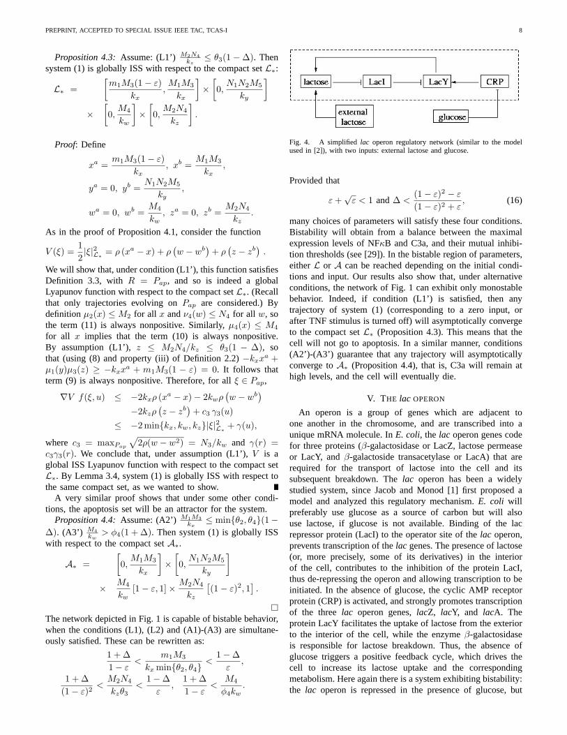
Fig. 4. A simplified lac operon regulatory network (similar to the modelused in [2]), with two inputs: external lactose and glucose.

Provided that

ε +√

ε < 1 and∆ <(1− ε)2 − ε

(1− ε)2 + ε, (16)

many choices of parameters will satisfy these four conditions.Bistability will obtain from a balance between the maximalexpression levels of NFκB and C3a, and their mutual inhibi-tion thresholds (see [29]). In the bistable region of parameters,eitherL or A can be reached depending on the initial condi-tions and input. Our results also show that, under alternativeconditions, the network of Fig. 1 can exhibit only monostablebehavior. Indeed, if condition (L1’) is satisfied, then anytrajectory of system (1) (corresponding to a zero input, orafter TNF stimulus is turned off) will asymptotically convergeto the compact setL∗ (Proposition 4.3). This means that thecell will not go to apoptosis. In a similar manner, conditions(A2’)-(A3’) guarantee that any trajectory will asymptoticallyconverge toA∗ (Proposition 4.4), that is, C3a will remain athigh levels, and the cell will eventually die.

V. THE lac OPERON

An operon is a group of genes which are adjacent toone another in the chromosome, and are transcribed into aunique mRNA molecule. InE. coli, the lac operon genes codefor three proteins (β-galactosidase or LacZ, lactose permeaseor LacY, andβ-galactoside transacetylase or LacA) that arerequired for the transport of lactose into the cell and itssubsequent breakdown. Thelac operon has been a widelystudied system, since Jacob and Monod [1] first proposed amodel and analyzed this regulatory mechanism.E. coli willpreferably use glucose as a source of carbon but will alsouse lactose, if glucose is not available. Binding of the lacrepressor protein (LacI) to the operator site of thelac operon,prevents transcription of thelac genes. The presence of lactose(or, more precisely, some of its derivatives) in the interiorof the cell, contributes to the inhibition of the protein LacI,thus de-repressing the operon and allowing transcription to beinitiated. In the absence of glucose, the cyclic AMP receptorprotein (CRP) is activated, and strongly promotes transcriptionof the three lac operon genes,lacZ, lacY, and lacA. Theprotein LacY facilitates the uptake of lactose from the exteriorto the interior of the cell, while the enzymeβ-galactosidaseis responsible for lactose breakdown. Thus, the absence ofglucose triggers a positive feedback cycle, which drives thecell to increase its lactose uptake and the correspondingmetabolism. Here again there is a system exhibiting bistability:the lac operon is repressed in the presence of glucose, but

PREPRINT, ACCEPTED TO SPECIAL ISSUE IEEE TAC, TCAS-I 9

transcribed in the absence of glucose and presence of lactose.In [2], this regulatory system and its response to glucoseand a lactose analog was explored: there are two inputs tothe system. A schematic view of the system is shown inFig. 4, where “lactose” stands for intracellular lactose. Lettingx = [lactose], y = [LacY], w = [LacI], z = [CRP],u1 = [extracellular lactose] and u2 = [glucose], a model forthe system depicted in Fig. 4 is:

x = −kxx + ν1(y) + ν4(u1)y = −kyy + µ1(w)ν2(z) (17)

w = −kww + µ2(x)z = −kzz + µ3(u2)

To simplify notation, letξ = (x, y, w, z)′ and let ξ = f(ξ, u)denote system (17). By Lemma 3.6, system (17) isPlac-forward complete. where:

Plac =[0,

N1 + N4

kx

]×

[0,

M1N2

ky

]×

[0,

M2

kw

]×

[0,

M3

kz

].

As in the apoptosis example, conditions can be given thatguarantee the capacity for bistable behavior. It is convenientto rewrite the equation forz, using Fact 1:

z = −kzz + M3 + (µ3(u)−M3)= −kzz + M3 − ν3(u), (18)

where N3 = M3. In Proposition 5.1 below, the setLlac

represents the response of thelac operon in the presence ofglucose: LacI (w) represses transcription of thelac genes, andonly a residual concentration of lactose (x) is present insidethe cell.

Proposition 5.1:Assume that (L1)εM1N2ky

< φ1(1 − ∆),

(L2) M2(1−ε)kw

> θ1(1 + ∆), and (L3) εN1kx

< θ2(1−∆). Thensystem (17) is locally ISS with respect to the compact set:

Llac =[0,

εN1

kx

]×

[0,

εM1N2

ky

]× M2

kw[1− ε, 1]×

[0,

M3

kz

].

Proof: By Lemma 3.4, it is enough to show that there existsa local ISS Lyapunov function with respect toLlac. Define

xa = 0, xb =εN1

kx, ya = 0, yb =

εM1N2

ky,

wa =M2(1− ε)

kw, wb =

M2

kw.

Following (6), consider the function:

V (ξ) =12|ξ|2Llac

= ρ(x− xb

)+ ρ

(y − yb

)+ ρ (wa − w) .

This function satisfies property (i) of Definition 3.3, and wewill show that it also satisfies property (ii). Findδ ∈ (0, 1) sothat:

(1 + δ)εM1N2

ky< φ1(1−∆),

δM2(1− ε)

kw> θ1(1 + ∆), (1 + δ)

εN1

kx< θ2(1−∆)

(such aδ exists, since (L1)-(L3) are strict inequalities), anddefine the following set :

R = {ξ ∈ Plac : x ≤ (1 + δ)xb, y ≤ (1 + δ)yb, δwa ≤ w}.

This setR clearly containsLlac in its interior (in the sensedefined by (3)). Then

∇V f(ξ, u) =√

2ρ (x− xb)(−kxx + ν1(y))

+√

2ρ (y − yb)(−kyy + µ1(w)ν2(z))

−√

2ρ (wa − w)(−kww + µ2(x))

+ν4(u1)√

2ρ (x− xb).

Noticing that−kxx + ν1(y) = −kx(x− xb)− kxxb + ν1(y),and that

√2ρ(x− xb)(x−xb) = 2kxρ(x−xb), the expression

∇V f(ξ, u) can be rewritten as

∇V f(ξ, u) = −2kx ρ(x− xb

)− 2ky ρ

(y − yb

)−2kw ρ (wa − w) + gx,b + gy,b + gw,a

+ν4(u1)√

2ρ (x− xb),

where

gx,b =√

2ρ (x− xb)(−kxxb + ν1(y)) (19)

gy,b =√

2ρ (y − yb)(−kyyb + µ1(w)ν2(z)) (20)

gw,a = −√

2ρ (wa − w)(−kwwa + µ2(x)). (21)

Now, let ξ ∈ R. Recall the definition ofδ. Theny < φ1(1−∆) implies (definition of activation function)ν1(y) < εN1,and hencegx,b ≤ 0. The fact thatw > θ1(1 + ∆) impliesµ1(w) < εM1 (by definition of an inhibition function), and so−kyyb+µ1(w)ν2(z) < −ky(yb−εM1N2/ky) = 0, andgy,b ≤0. Sincex < θ2(1 −∆) it follows that µ2(x) > M2(1 − ε),and−kwwa + µ2(x) > −kwwa + M2(1 − ε) = 0, so alsogw,a ≤ 0. Thus, the terms (19)-(21) are nonpositive. For theinput term, use Fact 2 to obtain aK∞ functionγ4(r) ≥ ν4(r).In conclusion, for all points ofR one can write:

∇V f(ξ, u) ≤ −2 min{kx, ky, kw}|ξ|2Llac+ γ(|u|),

whereγ(r) = (N1(1− ε)+N4)γ4(r)/kx is aK∞ function.In the next Proposition, the setAlac represents the state of

the operon in the absence of glucose and presence of externallactose. In this mode, both internal lactose and the Lac proteinsare present, while the repressor LacI is at a low level.

Proposition 5.2:Assume: (A1)M1N2(1−ε)2

ky> φ1(1 + ∆),

(A2) εM2kw

< θ1(1−∆), (A3) N1(1−ε)kx

> θ2(1+∆), and (A4)M3(1−ε)

kz> φ2(1 + ∆). Then system (17) is locally ISS with

respect to the compact set:

Alac =N1

kx[1− ε, 1]× M1N2

ky

[(1− ε)2, 1

]×

[0,

εM2

kw

]× M3

kz[1− ε, 1] .

Proof: The argument is very similar to that used in Propo-sition 5.1. Following (6), consider the function12 |ξ|

2Alac

:

V (ξ) = ρ (xa − x) + ρ(x− xb

)+ ρ (ya − y)

+ ρ(w − wb

)+ ρ (za − z) .

PREPRINT, ACCEPTED TO SPECIAL ISSUE IEEE TAC, TCAS-I 10

This function satisfies property (i) of Definition 3.3, andwe will show that it also satisfies property (ii). To simplifynotation, letξ = (x, y, w, z)′ and define

xa =N1(1− ε)

kx, xb =

N1

kx,

ya =M1N2(1− ε)2

ky, yb =

M1N2

ky,

wa = 0, wb =M2ε

kw, za =

M3(1− ε)kz

, zb =M3

kz.

Find δ ∈ (0, 1) so that:

δ(1− ε)2M1N2

ky> φ1(1−∆),

(1 + δ)M2ε

kw< θ1(1 + ∆), δ

(1− ε)N1

kx> θ2(1−∆),

δM3(1− ε)

kz> φ2(1 + ∆),

and define the following set:

R = {ξ ∈ Plac : δxa ≤ x, δya ≤ y,

w ≤ (1 + δ)wb, δza ≤ z}. (22)

This setR clearly containsAlac in its interior (in the sensedefined by (3)). Then computing and simplifying∇V f(ξ, u):

∇V f(ξ, u) = −2kx ρ (xa − x)− 2kx ρ(x− xb

)−2ky ρ (ya − y)− 2kw ρ

(w − wb

)−2kz ρ (za − z)+gx,a + gx,b + gy,a + gw,b + gz,a

+ν4(u1)(√

2ρ (xa − x) +√

2ρ (x− xb))

+ν3(u2)√

2ρ (za − z)

where

gx,a = −√

2ρ (xa − x)(−kxxa + ν1(y)) (23)

gx,b =√

2ρ (x− xb)(−kxxb + ν1(y)) (24)

gy,a = −√

2ρ (ya − y)(−kyya + µ1(w)ν2(z)) (25)

gw,b =√

2ρ (w − wb)(−kwwb + µ2(x)) (26)

gz,a = −√

2ρ (za − z)(−kzza + M3). (27)

Now, let ξ ∈ R. Recall the definition ofδ. Note first that−kzz

a + M3 > 0, and sogz,a < 0. Then y > φ1(1 + ∆)implies ν1(y) > (1 − ε)N1, and hence−kxxa + ν1(y) >−kxxa + N1(1 − ε) = 0, so thatgx,a ≤ 0. Note also that−kxxb + ν1(y) ≤ −kxxb + N1 = 0, so that gx,b ≤ 0.The fact thatx > θ2(1 + ∆) implies thatgw,b ≤ 0. Nownote that w < θ1(1 − ∆) implies µ1(w) > (1 − ε)M1

and z > φ2(1 + ∆) implies ν2(z) > (1 − ε)N2. Thus−kyya + µ1(w)ν2(z) > −kyya + M1N2(1 − ε)2 = 0 andgy,a ≤ 0. Thus, the terms (23)-(27) are nonpositive. For theinput term, use Fact 2 to obtain aK∞ functionγi(r) ≥ νi(r),i = 3, 4. In conclusion, for all points ofR one can write:

∇V f(ξ, u) ≤ −2 min{kx, ky, kw, kz}|ξ|2Alac+ γ(|u|),

where we usedui ≤ |u| =√

u21 + u2

2 for i = 1, 2, andγ(r) =M3(1 − ε)γ3(r)/kz + (N1(1 − ε) + N4)γ4(r)/kx is a K∞function.

More restrictive conditions can be given, for a monostablesystem. The next Proposition describes conditions under whichthe system is prevented from expressing high levels of the Lacproteins (and consequently cannot increase its lactose levels),whether or not glucose is available.

Proposition 5.3:Assume: (L1’) M1N2ky

≤ φ1(1 − ∆) and

(L2’) M2kw

≥ θ1(1+∆). Then system (17) is globally ISS withrespect to the compact set:

Llac,∗ =[0,

εN1

kx

]×

[0,

εM1N2

ky

]×

[0,

M2

kw

]×

[0,

M3

kz

].

Proof: Set

xa = 0, xb =εN1

kx, ya = 0, yb =

εM1N2

ky.

Consider the function:

V (ξ) =12|ξ|2Llac,∗

= ρ(x− xb

)+ ρ

(y − yb

).

It is easy to see that Lemma 3.4 can be applied withR = Plac.Indeed, note that

∇V f(ξ, u)

≤ −2kx ρ(x− xb

)+

√2ρ (x− xb)(−kxxb + ν1(y))

−2ky ρ(y − yb

)+

√2ρ (y − yb)(−kyyb + N2µ1(w))

+ν4(u1)√

2ρ (x− xb).

Assumption (L1’) (and recalling the definition of an activationfunction ν) implies that−kxxb + ν1(y) ≤ −kxxb + εN1 = 0.Assumption (L2’) implies that−kyyb +N2µ1(w) ≤ −kyyb +εN2M1 = 0. Therefore, using Fact 2, one can find aK∞function γ such that

∇V f(ξ, u) ≤ −2 min{kx, ky} |ξ|2Llac,∗+ γ(|u|)

and Property (ii) of Lemma 3.4 is satisfied.A similar argument shows that, under alternative condi-

tions, the Lac proteins will always be expressed and lactosemetabolism “switched on”, independently of glucose concen-tration. Not surprisingly, the conditions are opposite to thosegiven in Proposition 5.3.

Proposition 5.4:Assume: (A1’) M1N2ky

≥ φ1(1+∆), (A2’)M2kw

≤ θ1(1−∆), and Then system (17) is globally ISS withrespect to the compact set:

Alac,∗ =N1

kx[1− ε, 1]× M1N2

ky[1− ε, 1]

×[0,

M2

kw

]×

[0,

M3

kz

].

�Just as in the example of the apoptosis network, thelac

operon system clearly has the capacity for bistable response.This happens when the conditions from Propositions 5.1

PREPRINT, ACCEPTED TO SPECIAL ISSUE IEEE TAC, TCAS-I 11

and 5.2 are simultaneously satisfied. Putting conditions (L1)-(L3) and (A1)-(A4) together, one has:

N1

kxθ2,

M2

kwθ1∈

(1 + ∆1− ε

,1−∆

ε

)M1N2

kyφ1∈

(1 + ∆

(1− ε)2,1−∆

ε

)(28)

M3

kzφ2∈

(1 + ∆1− ε

,∞)

.

Note that assumption (A4) (condition onkz) simply reflectsthe fact that the input functionµ3 should have a sufficientlyhigh maximal production rate: for low levels of glucose, theprotein CRP should become activated. It is necessary thatε <1/2 for Llac andAlac to be disjoint sets. In addition, bothεand∆ should satisfy the condition (16) (as for the apoptosisnetwork).

If glucose is available andµ3(u) ≈ 0, then thelac operonactivator (CRP) is not activated. The system will be evolving inthe setLlac. Suppose now that glucose is all used up: then theactivator CPR enables and amplifies transcription of the operongenes. A nonzero input of extracellular lactose, together withthe positive feedback loop, will repress LacI and inducesucessful transcription of thelac operon. The system willeventually be driven to the setAlac. (see Section V-B below).The conditions listed in Propositions 5.3 or 5.4 represent twosituations where bistability is not possible. In the absence ofinputs, the trajectoriesalwaysconverge to the setLlac,∗ (resp.,Alac,∗), which correspond to the mode of repressed (resp.,induced)lac operon.

A. Comparison to experimental results

The result of Proposition 5.4 can be compared to anexperiment reported in [2]. In this paper, the authors detect andmeasure the bistable response of thelac operon. In one of theexperiments, a new strain ofE. coli was constructed, whichhas extra LacI binding sites introduced. Adding new LacIbinding sites is equivalent to increasing the activity thresholdθ1, because a larger number of LacI molecules will be neededto produce the same level of repression of the operon. Thisnew strain ofE. coli was then exposed to increasing levelsof extracellular TMG (a non-metabolizable lactose analogue).Increasing the levels of extracellular lactose corresponds todecreasing the activity thresholdφ1, since it becomes easierfor permease LacY to recruit lactose. Thus it holds that• increasing the levels of extracellular lactose (∼ 1/φ1)

leads to validation of condition (A1’);• a large increase in LacI binding sites (∼ θ1) validates

condition (A2’).According to Proposition 5.4, the mode “repressedlac operon”is not stable for this new strain. And indeed, the experiment(see [2], Fig. 4c) shows that only one qualitative type ofresponse can be obtained from this strain, corresponding tothe inducedlac operon – as characterized byAlac,∗.

B. Controlling the system towards lactose metabolism

A fundamental problem in the analysis of bistable biologicalsystems is that of controlling or switching the system from one

stable mode to another. In many cases, while possible inputs orstimuli are known (for instance, TNF in the apoptosis network;or extracellular lactose or glucose in thelac operon), it isnot always clear how to “design” the control that will drivethe system to the desired state. Following our idea that eachdesired state is represented by a set (as opposed to a singlestationary point), our results suggest one method to control thesystem towards a desired setQ: first, “turn on” the stimulusuntil the system is in a sufficiently small neighborhood ofQ, and then “turn off” stimulus. This is a reasonable protocolfrom the experimental point of view, as cell stimulation is oftenachieved through piecewise constant inputs: for instance, thecells are maintained in a medium with fixed external lactoseand glucose concentrations (sayE andG), for a certain timeinterval (sayt ∈ [t0, t0 + T ]).

For instance, to switchE. coli to the lactose metabolismmode (Alac), glucose and external lactose should, respectively,be removed from and added to the system, and maintainedat, respectively, low and high levels, fora suitable periodof time. To switch off lactose metabolism and go back toglucose metabolism (Llac), it suffices to add an appropriateamount of glucose to the medium and again wait for asufficiently long interval. Thus, the question of choosing anappropriate stimulation intervalarises or, more generally,choosing appropriate combinations ofE, G andT . The nextProposition provides an answer to this question, by fixing aminimum time interval needed to start lactose metabolism.

Assume that the bistability conditions (28) are satisfied.Assume further that

N4 > N1. (29)

Let E0 < φ4(1 + ∆) and G0 < θ3(1 − ∆), and considerconstant inputs of the form:

u1(t) = E0, u2(t) = G0, t ∈ [0, T ], (30)

andu1(t) = u2(t) = 0 for t > T . Let δ ∈ (0, 1) andR be theset constructed in the proof of Proposition 5.2, and define:

T1 = − 1kx

ln(

1− kxθ2

N4

1 + ∆1− ε

)T2 = − 1

kxln

(1− N1

N4

)T3 = T1 −

1kw

lnε

1− ε

(kwθ1

M2

1−∆ε

− 1)

T4 = T1 −1

kwln

ε

1− ε

(1 + δ

ε− 1

)T5 = − 1

kzln

(1− kzφ2

M3

1 + ∆1− ε

)T6 = − 1

kzln (1− δ)

T7 = max{T3, T5} −1ky

ln (1− δ) .

By assumptions (28), (29), andε < 1/2, it follows that allarguments inside the logarithms are positive and less than 2.Put

T∗ = max{T2, T4, T6, T7}.

PREPRINT, ACCEPTED TO SPECIAL ISSUE IEEE TAC, TCAS-I 12

The next result shows that stimulus should be on for at leastT = T∗, in order to drive thelac operon to switch from lactoseto glucose metabolism modes.

Proposition 5.5:Let ξ(t, ξ0, u) be the solution of sys-tem (17) with initial conditionξ0 ∈ Llac, and input (30).Then ξ(t, ξ0, u) evolves in the setR (containingAlac), forT∗ < t ≤ T .

Proof: We will show that, forT∗ ≤ t ≤ T , the trajectoryevolves inside the setR. For t ∈ [0, T ], for an input of theform (30), it is clear thatx ≥ −kxx + (1 − ε)N4 and z ≥−kzz + (1 − ε)M3, so that (one may assume, in the worstcase, thatx0 = z0 = 0):

x(t) ≥ (1− ε)N4

kx(1− e−kxt)

z(t) ≥ (1− ε)M3

kz(1− e−kzt).

It is straigthforward to check that:

T1 < t ≤ T ⇒ x(t) > θ2(1 + ∆) (31)

T2 < t ≤ T ⇒ x(t) > (1− ε)N1/kx (32)

T5 < t ≤ T ⇒ z(t) > φ2(1 + ∆) (33)

T6 < t ≤ T ⇒ z(t) > δ(1− ε)M3/kz. (34)

Coordinatew starts decreasing asx increases aboveθ2(1+∆):

w(t) ≤ M2

kwe−kw(t−T1) +

εM2

kw(1− e−kw(t−T1)),

and hence:

T3 < t ≤ T ⇒ w(t) ≤ θ1(1−∆) (35)

T4 < t ≤ T ⇒ w(t) ≤ (1 + δ)εM2

kw. (36)

Expression (35) and (33) imply thaty ≥ −kyy + M1N2(1−ε)2, for max{T3, T5} < t ≤ T and so, in this time interval,

y(t) ≥ (1− ε)2M1N2

ky(1− e−ky(t−T3,5)).

It is clear now thatT7 < t ≤ T implies y(t) ≥ δ (1−ε)2M1N2ky

.This together with (32), (34), and (36) finishes the proof.

As indicated by this Proposition, external lactose is neededto “switch” the system from glucose to lactose metabolism(Llac to Alac). Indeed, glucose should be absent and externallactose available, during a minimum length of time,T∗. Theinverse switch (Alac to Llac) would be obtained by invertingthe input conditions (i.e., high glucose, low external lactose).

VI. D ISCUSSION

The examples discussed in Sections IV and V illustratea general formalism for modeling genetic networks, using aclass of inhibition and activation functions. These functionsare defined by appropriate physiological bounds, and allowthe mathematical model to capture the variability often en-countered in biological systems. Using this formalism, thepossible responses of the network to various stimuli canbe characterized by identifying invariant sets of the model.The goal is to identify invariant sets that represent distinctqualitative modes of operation of the system. For instance,

the capacity of the network to exhibit bistable behavior ischaracterized by the co-existence of two disjoint (compactand nonempty) invariant subsets of the state space (namedLandA in the examples), with low versus high concentrationsof some species. Each of these invariant subsets is describedby conditions on the parameters (relating maximal activities,activity thresholds and degradation constants), and representsa distinct response of the network: life or cell death innetwork (1), andlac operon repression or transcription innetwork (17). In all examples, it is shown that the system islocally ISS with respect to bothL andA. This ISS propertyleads to 0-invariance, that is in the absence of an input, ifthe system starts in one of the sets, then it will remain inthat set. Since there are at least two such invariant sets, thesystem is indeed capable of operating in two distinct modes,in a stable manner. Furthermore, inputs or perturbations ofsmall magnitude (as given by the corresponding setsR) do notdrive the system far out from the 0-invariant set. Therefore, thesystem exhibits robustness with respect to small fluctuationsin the environment, as its qualitative response is basicallyunchanged.

In contrast, conditions on the parameters that guaranteemonostability are also given. Monostability is characterizedby the existence of a 0-invariant set (denoted by eitherL∗or A∗ in the examples), with respect to which the system isglobally ISS. Global ISS with respect to a given compact setL∗ guarantees that, in the absence of an input, the trajectoriesof the system asymptotically converge toL∗, independently ofthe initial condition, which rules out the capacity for a bistableresponse of the network.

In both biological systems discussed, the wild type healthycell has the capacity for bistability, that is, it can respond intwo distinct ways, in a stable manner. However, damaged ormalfunctioning cells often loose the capacity for bistability.This happens in the apoptosis network [33], where damagedcells seem to loose the capacity to undergo apoptosis, causingvarious diseases. It has also been verified for thelac operon onspecially constructed strains ofE. coli, as in [2] (Section V-A).The conditions developed in Propositions 4.1, 4.3, and 4.2, 4.4,provide a means to classify cells, according to whether they arehealthy (both (L1)-(L3) and (A1)-(A4) satisfied), or not (either(L1’)-(L2’) or (A1’)-(A2’)). For example, Proposition 4.4describes a malfunctioning cell, such as a cancerous cell(condition (L1’), low levels of C3a). And we have seen inSection V that Proposition 5.4 correctly describes anE. colistrain with extra LacI binding sites.

Our analysis can thus be applied to the detection of malfunc-tioning or damaged cells. (Note that, if none of the conditionsis satisfied, then our analysis is not conclusive). By measuringthe maximal production rates, as well as degradation ratesand activation/inhibition thresholds for a given network, onecan then check which of the conditions (L1)-(L3), (L1’)-(L2’)and (A1)-(A4), (A1’)-(A2’) are satisfied. Once the system isthus classified, an appropriate input can be constructed, tocontrol the system to a desired compact set. Observe that ifthe system (1) is in the living stateL, then by sufficientlyincreasing TNF (and appropriate conditions onµ5, ν3) itis possible to drive the system towards apoptosis. Once the

PREPRINT, ACCEPTED TO SPECIAL ISSUE IEEE TAC, TCAS-I 13

trajectory reaches the setA (or sufficiently close), the stimuluscan be “turned off” and the trajectory will remain in theset A (or expected to converge towardsA, if in its basinof attraction). On the other hand, if the system starts in theapoptosis setA, then no input will drive the system backtowards the “living” state – which of course makes sensefrom the biogical point of view. In thelac operon network(Proposition 5.5), it is interesting to note thattwo independentinputs are needed to allow the system to switch between thetwo stable modes, in both directions.

VII. C ONCLUSION

A general framework has been discussed for modelinggenetic regulatory networks, where interactions among genesand proteins are described in terms of a class of free-formactivation and inhibition functions. The formalism presentedin this paper intuitively relates the class of piecewise linearhybrid models to a class of continuous models: one possibleextension of the formalism is to explore this connection tofurther study and analyze piecewise linear models. Otherpossible extensions of the current work include introducingmore general degradation functions.

The capacity for mono- or bi-stable behavior in a geneticregulatory network can be fully characterized by identifyingappropriate 0-invariant compact sets for the system (withrespect to which the system is, respectively, globally or locallyinput-to-state stable). Conditions relating the degradation rates,maximal activities and threshold constants are provided, whichguarantee that the system will be capable of bistable or onlymonostable behavior. Our analysis allows a classification ofsystems (or cells) according to their capacity for monostableor bistable responses. This classification helps to distinguishamong “healthy” and “damaged” or “malfunctioning” cells.An application of this knowledge is the construction of suitableinputs (stimuli) that will drive the system to a desired compactset – and drive the biological network to a desired qualitativeresponse.

REFERENCES

[1] F. Jacob and J. Monod, “Genetic regulatory mechanisms in the synthesisof proteins,”J. Mol. Biol., vol. 3, pp. 318–356, 1961.

[2] E. Ozbudak, M. Thattai, H. Lim, B. Shraiman, and A. van Oudenaarden,“Multistability in the lactose utilization network ofEscherichia coli,”Nature, vol. 427, pp. 737–740, 2004.

[3] M. Ptashne,A genetic switch: phageλ and higher organisms. CellPress & Blackwell scientific publications, 1992.

[4] N. Danial and S. Korsmeyer, “Cell death: critical control points,”Cell,vol. 116, pp. 205–216, 2004.

[5] A. Hoffmann, A. Levchenko, M. Scott, and D. Baltimore, “The IkB-NFkB signaling module: temporal control and selective gene activation,”Science, vol. 298, pp. 1241–1245, 2002.

[6] T. Eißing, H. Conzelmann, E. Gilles, F. Allgower, E. Bullinger, andP. Scheurich, “Bistability analysis of a caspase activation model forreceptor-induced apoptosis,”J. Biol. Chem., vol. 279, pp. 36 892–36 897,2004.

[7] J. Pomerening, E. Sontag, and J.E. Ferrell, Jr., “Building a cell cycleoscillator: hysteresis and bistability in the activation of Cdc2,”Nat. CellBiol., vol. 5, pp. 346–351, 2003.

[8] T. Eißing, F. Allgower, and E. Bullinger, “Robustness properties ofapoptosis models with respect to parameter variations and stochasticinfluences,”IEE Proc. Syst. Biol., vol. 152, pp. 221–228, 2005.

[9] D. Angeli, J.E. Ferrell, Jr., and E. Sontag, “Detection of multistability,bifurcations and hysteresis in a large class of biological positive-feedback systems,”Proc. Natl. Acad. Sci. USA, vol. 101, pp. 1822–1827,2004.

[10] J. Vilar, C. Guet, and S. Leibler, “Modeling network dynamics: thelacoperon, a case study,”J. Cell Biol., vol. 161, pp. 471–476, 2003.

[11] A. Arkin, J. Ross, and H. McAdams, “Stochastic kinetic analysis ofdevelopmental pathway bifurcation in phageλ-infectedescherichia colicells,” Genetics, vol. 149, pp. 1633–1648, 1998.

[12] M. Khammash and H. El Samad, “Stochastic modeling and analysisof genetic networks,” inProc. 44th IEEE Conf. Decision and Control,Seville, Spain, 2005.

[13] R. Thomas, “Boolean formalization of genetic control circuits,”J. Theor.Biol., vol. 42, pp. 563–585, 1973.

[14] L. Sanchez and D. Thieffry, “A logical analysis of thedrosophilagap-gene system,”J. Theor. Biol., vol. 211, pp. 115–141, 2001.

[15] R. Albert and H. Othmer, “The topology of the regulatory interactionspredicts the expression pattern of thedrosophilasegment polarity genes,”J. Theor. Biol., vol. 223, pp. 1–18, 2003.

[16] M. Chaves, R. Albert, and E. Sontag, “Robustness and fragility ofboolean models for genetic regulatory networks,”J. Theor. Biol., vol.235, pp. 431–449, 2005.

[17] R. Ghosh and C. Tomlin, “Symbolic reachable set computation of piece-wise affine hybrid automata and its application to biological modeling:Delta-notch protein signaling,”IEE Trans. Syst. Biol., vol. 1, pp. 170–183, 2004.

[18] L. Glass and S. Kauffman, “The logical analysis of continuous, nonlinearbiochemical control networks,”J. Theor. Biol., vol. 39, pp. 103–129,1973.

[19] H. de Jong, J. Gouze, C. Hernandez, M. Page, T. Sari, and J. Geiselmann,“Qualitative simulation of genetic regulatory networks using piecewiselinear models,”Bull. Math. Biol., vol. 66, pp. 301–340, 2004.

[20] R. Casey, H. de Jong, and J. Gouze, “Piecewise-linear models of geneticregulatory networks: equilibria and their stability,”J. Math. Biol., vol. 52,pp. 27–56, 2006.

[21] E. Farcot, “Geometric properties of a class of piecewise affine biologicalnetwork models,”J. Math. Biol., vol. 52, pp. 373–418, 2006.

[22] M. Chaves, E. Sontag, and R. Albert, “Methods of robustness analysisfor boolean models of gene control networks,”IEE Proc. Syst. Biol.,vol. 153, pp. 154–167, 2006.

[23] H. de Jong and D. Thieffry, “Modelisation, analyse et simulation desreseaux genetiques,”Medecine/Sciences, vol. 18, pp. 492–502, 2002.

[24] E. Sontag and Y. Wang, “On characterizations of the input-to-statestability property with respect to compact sets,” inProc. IFAC NonlinearControl Symposium (NOLCOS95), Tahoe City, CA, 1995.

[25] E. Sontag, “Smooth stabilization implies coprime factorization,”IEEETrans. Automat. Control, vol. 34, pp. 435–443, 1989.

[26] E. Sontag and Y. Wang, “On characterizations of the input-to-statestability property,”Systems Control Lett., vol. 24, pp. 351–359, 1995.

[27] M. Chaves and E. Sontag, “State-estimators for chemical reaction net-works of Feinberg-Horn-Jackson zero-deficiency type,”Eur. J. Control,vol. 8, pp. 343–359, 2002.

[28] M. Chaves, “Input-to-state stability of rate-controlled biochemical net-works,” SIAM J. Control Optim., vol. 44, pp. 704–727, 2005.

[29] M. Chaves, T. Eißing, and F. Allgower, “Identifying mechanisms forbistability in an apoptosis network,” inReseaux d’interactions : anal-yse, modelisation et simulation, ser. Integrative Post-Genomics, Lyon,France, 2006.

[30] M. Krichman, E. Sontag, and Y. Wang, “Input-output-to-state stability,”SIAM J. Control Optim., vol. 39, pp. 1874–1928, 2001.

[31] M. Arcak, D. Angeli, and E. Sontag, “A unifying integral iss frameworkfor stability of nonlinear cascades,”SIAM J. Control Optim., vol. 40, pp.1888–1904, 2002.

[32] M. Schliemann, T. Eissing, P. Scheurich, and E. Bullinger, “Mathemati-cal modelling of TNF-α induced apoptotic and anti-apoptotic signallingpathways in mammalian cells based on dynamic and quantitative experi-ments,” in2nd Foundations of Systems Biology in Engineering (FOSBE),Stuttgart, Germany, 2007, in press.

[33] T. Eißing, S. Waldherr, E. Bullinger, C. Gondro, O. Sawodny,F. Allgower, P. Scheurich, and T. Sauter, “Sensitivity analysis of pro-grammed cell death and implications for crosstalk phenomena duringTumor Necrosis Factor stimulation,” inIEEE Conf. Control Applications(CCA), Munich, Germany, 2006, pp. 1746–1752.

PREPRINT, ACCEPTED TO SPECIAL ISSUE IEEE TAC, TCAS-I 14

Madalena Chaves joined the Institut National deRecherche en Informatique et en Automatique (IN-RIA) Sophia Antipolis, France, in 2007. She re-ceived her Licenciatura in Technological Physicsin 1995, from Instituto Superior Tecnico, Lisbon,Portugal and her Ph.D. in Mathematics in 2003,from Rutgers University, New Jersey. She was avisiting scientist at Sanofi-Aventis, New Jersey, fortwo years, and then held a post-doctoral position atthe Institute for Systems Theory and Automatic Con-trol, University of Stuttgart, Germany. Her research

interests include the analysis of dynamical systems, stability and robustnessof nonlinear systems, modeling and analysis of biological regulatory networksand signaling pathways.

Thomas Eissing studied life science and biotechnol-ogy at the Universities of Stuttgart (Germany) andNew South Wales (Australia). In 2002 he joined theInstitute for Systems Theory and Automatic Controlas a research assistant and PhD student in the areaof systems biology, expecting his degree in 2007.During his studies, he held short-term visiting posi-tions with Millennium Pharmaceuticals, Inc. (USA)and the Hamilton Institute (Ireland). Since 2007, hecontinues his systems biology interests working withBayer Technology Services (Germany).

Frank Allgwer is director of the Institute for Sys-tems Theory in Engineering and professor in theMechanical Engineering Department at the Univer-sity of Stuttgart in Germany. He studied EngineeringCybernetics and Applied Mathematics at the Uni-versity of Stuttgart and the University of Californiaat Los Angeles respectively. He received his Ph.D.degree in Chemical Engineering from the Universityof Stuttgart. Prior to his present appointment heheld a professorship in the electrical engineeringdepartment at ETH Zurich. He also held visiting

positions at Caltech, the NASA Ames Research Center, the DuPont Companyand the University of California at Santa Barbara.

His main interests in research and teaching are in the area of systems andcontrol with emphasis on the development of new methods for the analysisand control of nonlinear systems and the identification of nonlinear systems.Of equal importance to the theoretical developments are practical applicationsand the experimental evaluation of benefits and limitations of the developedmethods. Applications range from chemical process control and control ofmechatronic systems to AFM control and systems biology.

Frank Allgower is Editor for the journal Automatica, Associate Editor ofthe Journal of Process Control and the European Journal of Control and is onthe editorial board of several further journals including the Journals of Robustand Nonlinear Control and Chemical Engineering Science. Among others hecurrently serves on the scientific council of the Gesellschaft fur Mess- undAutomatisierungstechnik, is member of the council of the European UnionControl Association and is chairman of the IFAC Technical committee onNonlinear Systems. He is organizer or co-organizer of several internationalconferences and has published over 100 scientific articles. Frank receivedseveral prizes for his work including the Leibniz prize, which is the mostprestigious prize in science and engineering awarded by the German NationalScience Foundation (DFG).