1

STATE TRANSITION MATRIX FOR PERTURBED ORBITAL MOTION USING MODIFIED CHEBYSHEV PICARD ITERATION

Julie Read,* Ahmad Bani-Younes+, John L. Junkins†, and James Turner‡

The Modified Chebyshev Picard Iteration (MCPI) method has recently proven to

be more efficient for a given accuracy than the most commonly adopted numeri-

cal integration methods, as a means to solve for perturbed orbital motion. This

method utilizes Picard iteration, which generates a sequence of path approxima-

tions, and discrete Chebyshev Polynomials, which are orthogonal and also ena-

ble both efficient and accurate function approximation. The nodes consistent

with discrete Chebyshev orthogonality are generated using cosine sampling; this

strategy also reduces the Runge effect and as a consequence of orthogonality,

there is no matrix inversion required to find the basis function coefficients. The

MCPI algorithms considered herein are parallel-structured so that they are im-

mediately well-suited for massively parallel implementation with additional

speedup.

MCPI has a wide range of applications beyond ephemeris propagation, includ-

ing the propagation of the State Transition Matrix (STM) for perturbed two-

body motion. A solution is achieved for a spherical harmonic series representa-

tion of earth gravity (EGM2008), although the methodology is suitable for ap-

plication to any gravity model. Included in this representation is a derivation of

the second partial derivatives of the normalized, Associated Legendre Functions,

which is given and verified numerically.

INTRODUCTION

The Modified Chebyshev-Picard Iteration (MCPI) method is used to solve both linear and

nonlinear, high precision, long-term orbit propagation problems through iteratively finding an

orthogonal function approximation for the entire state trajectory. At each iteration, MCPI finds an

entire path integral solution, as opposed to the conventional, incremental step-by-step solution

strategy of more familiar numerical integration strategies. A major advantage of the MCPI ap-

proach is that the use of cosine sampling reduces the well-known Runge Effect. This algorithm

has recently proven to be a powerful tool for solving nonlinear differential equations for both ini-

tial value problems (IVP) and boundary value problems (BVP).1,2,3,4,5

Comparisons with other

methods6,7

have shown that MCPI is more efficient for a prescribed solution accuracy. Signifi-

cantly, however, unlike conventional integration approaches, it is ideally suited for massive paral-

lel implementations that provide further boosts in the computational performance.

* PhD Student, Aerospace Engineering, Texas A&M University, 3141 TAMU, College Station, TX 77843. + Assistant Professor, Aerospace Engineering, Khalifa University, P.O. Box 127788, Abu Dhabi, UAE. † Distinguished Professor, Aerospace Engineering, Texas A&M University, 3141 TAMU, College Station, TX 77843. ‡‡ Visiting Professor, Aerospace Engineering, Khalifa University, P.O. Box 127788, Abu Dhabi, UAE.

(Preprint) AAS 15-008

2

Here we consider the MCPI method to compute the State Transition Matrix (STM) for the

case of perturbed motion, which has applications in many areas including celestial mechanics and

control systems. Propagation of the STM is useful in determining the sensitivity of the IVP solu-

tion to the initial conditions; for instance, the STM predicts how deviations from the desired ini-

tial conditions will cause the trajectory of a spacecraft to stray from a nominal path. The STM

may be used to compute the time evolution of a state vector even for nonlinear systems, such as

the two-body problem perturbed by spherical harmonic gravity. In cases where the initial devia-

tion is small at time , a linear approximation may be used to determine the deviation at time .

This linear approximation is generated using the STM, a matrix of partial derivatives for the in-

stantaneous position and velocity with respect to the initial position and velocity; this means that

the STM is initially equal to the identity matrix8,9

.

The computation of the STM for the spherical harmonic gravity model requires second partials

of the gravity potential with respect to spherical geocentric coordinates: radius, latitude, and lon-

gitude. These required partial derivatives include second partials of the normalized, Associated

Legendre Functions (ALFs). The normalized version of the ALFs is the preferred formulation

because the associated recursion used to compute these functions tends toward weak numerical

instability as a higher degree and order gravity model is used. The derivation for these expres-

sions, presented in this paper, is not given in the current literature. Once the normalized ALFs are

computed, the gravity and associated derivatives are computed in part by introducing a scale fac-

tor to find an un-normalized version of the ALFs. Since a spherical harmonic model is used and

this gravity potential is a rigorous solution of the Laplace equation, the ALF's second partial deri-

vation for an arbitrary order spherical harmonic series is verified using the Laplace equation.

Both the trajectory and the STM are computed in a rotating, Earth-centered, Earth-fixed frame,

which is transformed into an Earth-centered inertial frame (for subsequent integration) at each

iteration. We also check to confirm that the STM accurately satisfies (with maximum relative er-

rors of < in a Matlab implementation and up to one orbit, for the most precise tuning) the

theoretical STM group properties as well as the STM symplectic property associated with natural

conservative dynamical systems8. The present development of the STM is also verified using fi-

nite difference methods.

MODIFIED CHEBYSHEV PICARD ITERATION

MCPI is a fusion of Picard iteration with the set of orthogonal Chebyshev polynomials. A few

papers were published on the topic prior to the development of parallel computing capabili-

ties,10,11

but it was not until recent years that this area was significantly expanded by the research

group at Texas A&M University under the lead of Dr. John L. Junkins. MCPI is an iterative, path

approximation numerical integrator. The entire state trajectory arc is approximated at every itera-

tion until a specified tolerance is met2. Emile Picard stated that, given an initial condition

, any first order differential equation

(1)

with an integrable right hand side may be rearranged, without approximation into an integral:

(2)

Then a unique solution to the initial value problem may be found using an iterative sequence

of path approximations through Picard iteration as

3

(3)

where the integrand of the Picard iteration sequence is approximated using Chebyshev poly-

nomials. For further details on the basics of this novel integration technique and its convergence

properties, refer to References 1 and 2. Since the Chebyshev polynomials are orthogonal a matrix

inverse is avoided when finding basis function coefficients; this inverse is commonly used in

step-by-step methods. Because cosine sampling is employed for MCPI, the Runge Effect seen at

trajectory boundaries is significantly reduced. Also, initial efforts to implement MCPI using par-

allel computation have shown additional speedup12

.

The present study considers the gravity-perturbed acceleration , which may be rep-

resented in state space notation for the MCPI algorithm as

,

= (4)

BASIC EQUATIONS FOR STATE TRANSITION MATRIX

The differential equation we wish to integrate for the STM is8

(5)

where

we know that the STM is computed as partials of the state vector (for the present work, the

state consists of position and velocity for an Earth-orbiting satellite):

(9)

Then we can write the G matrix in terms of the partials of the generally perturbed gravitational

acceleration case; for example the partial of the first component of acceleration with respect to

the first component in a body-fixed frame is written with respect to geocentric radius, latitude,

and longitude:

(10)

Many of the intermediate partials may be computed once and used iteratively. The in-

dividual components of the matrix G may be written explicitly as described in the follow-

ing sections.

(6)

(7)

Because we wish to integrate , we next find an expression in terms of . Since by

definition,

, and using

(8)

4

STATE TRANSITION MATRIX USING SPHERICAL HARMONIC GRAVITY

A spherical harmonic gravity model is used for this development. The Jacobian of the acceler-

ation, needed for Eq. (6), is computed in the body frame but transformed into the inertial frame

prior to each integration step; this method is presented in the following section. The full gravita-

tional potential function is defined as13

where r is the radial distance to the object, is the geocentric latitude of the object, is the

longitude of the object, Re is the magnitude of Earth's equatorial radius, and are the Associ-

ated Legendre Functions. The spherical harmonic acceleration due to gravity in a body-fixed ref-

erence frame may then be represented as

(12)

The expressions comprising the acceleration function are written explicitly as

(13)

(14)

(15)

Next we find expressions needed to compute the Jacobian of the acceleration in Eq. (6).

The individual components of the gravity perturbed acceleration in the Earth-centered inertial

frame are

(16)

(17)

(18)

For the partial fraction expansions of the components of G, we use the general formula:

(19)

The individual components of G then follow a pattern. The first few expressions are given

here, where

,

, and

as given in Eqs. (12) - (14).

(11)

5

(20)

(21)

(22)

The spherical coordinate partials with respect to Cartesian coordinates are found to be

(23)

Then, the second partials of the gravity potential are found, where the partials of the ALFs are

given in the following section. The matrix of second partials is symmetric, and the expressions

are as follows:

(24)

(25)

(26)

(27)

(28)

6

(29)

COMPUTATION OF ASSOCIATED LEGENDRE FUNCTIONS

A key component of the spherical harmonic gravity calculations is the set of Associated Le-

gendre Functions, . These functions are related to the Legendre polynomials, .14

(30)

(31)

The equation for the gravity potential only contains a singularity at r = 0, but the

gravity force in spherical coordinates, given below, contains a singularity at the poles

.

(32)

For this reason, in many real-time applications the potential function is represented us-

ing the so-called derived Associated Legendre Functions.15

The derived ALFs are defined

as follows:

(33)

Unfortunately, the typical recursions used to compute the can lose accuracy for

many applications due to numerical errors arising during the recursive processing (see

Table 1 of Reference 14). To overcome this problem, the derived Associated Legendre

Functions and spherical harmonic coefficients are normalized to improve accuracy for

high degree and order gravity models. First, define as an un-normalized, derived As-

sociated Legendre Function and as a normalized, derived Associated Legendre Func-

tion as given in15

. Similarly, is an un-normalized, Associated Legendre Function,

while is a normalized, Associated Legendre Function. Since the spherical harmonics

correspond to a linear subspace of 2-D Fourier Series, a typical normalization factor is

found; from Ch. 3, formula (7) of Reference 6, the derived ALF may be expanded, giving

rise to a coefficient that generates numerically stable recursive calculations. This coeffi-

cient is often used in geodesy applications.14,17,18,20,21

Then, the normalized and un-

normalized, derived ALFs are related by this normalization, written generally for

as14

(34)

where the Kronecker delta function is defined to be

(35)

The recursion formula chosen for the current work is the normalized, derived Associat-

ed Legendre Functions from Table 2, option I of Reference 14 for :

7

(37)

(38)

(39)

These scale factors will be applied to the expressions as described in the following

subsection.

Computation of Partials of Associated Legendre Functions

Computation of the STM for the spherical harmonic gravity case requires the partial

derivative of with respect to , where and are the normalized Stokes coeffi-

cients determined from satellite motion observations, and is a scale factor described

in the previous section. The equation for this first partial is presented, then the second par-

tial of with respect to is derived in detail. The derivation for this second partial ex-

pression is not given in the current literature. The first and second partials of the ALFs are

incorporated in the calculations for the partials of the gravity potential, U, through the

computation of the corresponding ALFs and the appropriate scale factors. The following

known relationships will be used for these derivations.14

(40)

(41)

(42)

It is known that the derived ALFs are related to the conventional Legendre functions

in terms of latitude 14 through

(43)

Starting with the above equation and using the product rule,

(44)

(36)

Note that the specific cases of and may each use a more specific formu-

la for efficiency.

Since a normalized version of the ALFs is used, the final un-normalized result may be

obtained by applying the appropriate scale factor. For efficiency, the scale factor for

three cases are computed separately:

8

This equation can be rewritten using Eq. (43) as

(45)

Using Eqs. (42) and (43), the final equation becomes

(46)

Similarly, an expression for

may be derived.

(47)

Substituting Eq. (45) into this expression gives

(48)

Eq. (45) may also be used to write

(49)

Therefore, the final expression for the second partial is

(50)

In the code, the term is multiplied by the scale factor , and the term

is multiplied by the scale factor to compensate for the original

normalization of the ALFs. The final, normalized equations are then

(51)

(52)

Verification for Second Partial of ALF with Respect to Latitude

The second partial of the gravity potential with respect to geocentric latitude may be checked

since it is a rigorous solution of Laplace's equation21

:

(53)

9

which may be simplified as

(54)

This equation is compared numerically with Eq. (27) to confirm that the derivation for the second

partial of the ALF with respect to latitude is correct.22

See the next section for resulting plots.

SIMULATION RESULTS

First, to show that the derivation of the second partial of the ALFs is correct using the normal-

ization in MCPI, a finite difference approximation method is incorporated into the simulation. All

solutions were obtained using a 10th order gravity, Earth rotation of and

tolerances for the trajectory and STM, respectively, of 1e-8

and 1e-5

. As can be seen in Figure (1),

the first and second partials of the Legendre Functions match closely with the finite difference

check approximations (the partials use a normalization scheme as described in the present paper).

The ALFs and the first and second partials of the ALFs are computed as lower triangular matrices

that depend on and , which are the upper summation limits of Eq. (10). Therefore, the size of

these matrices are defined by user inputs.

Figure 1. Finite Difference Check for First and Second Partial Derivatives of ALFs.

Similarly, to verify that the formulation developed here for the STM is correct using MCPI, a fi-

nite difference check of both the second partials of the gravity potential and the STM matrix are

completed and give results comparable in accuracy to the figure above.

An additional verification of the second partial with respect to latitude, , uses the Laplace

Equation as described in the previous section. The second partial

obtained using this method

is compared with the second partial computed using the expression derived in Eq. (26), which is

directly a function of the ALFs. The result of this comparison is shown in Figs. (2) and (3). The

relative error plot shows spikes that are due to the second partial

approaching zero as a nor-

malization factor in the denominator.

10

Figure 2. Absolute Error Check for Second Partial of Gravity Potential with Respect to Latitude.

Figure 3. Relative Error Check for Second Partial of Gravity Potential with Respect to Latitude.

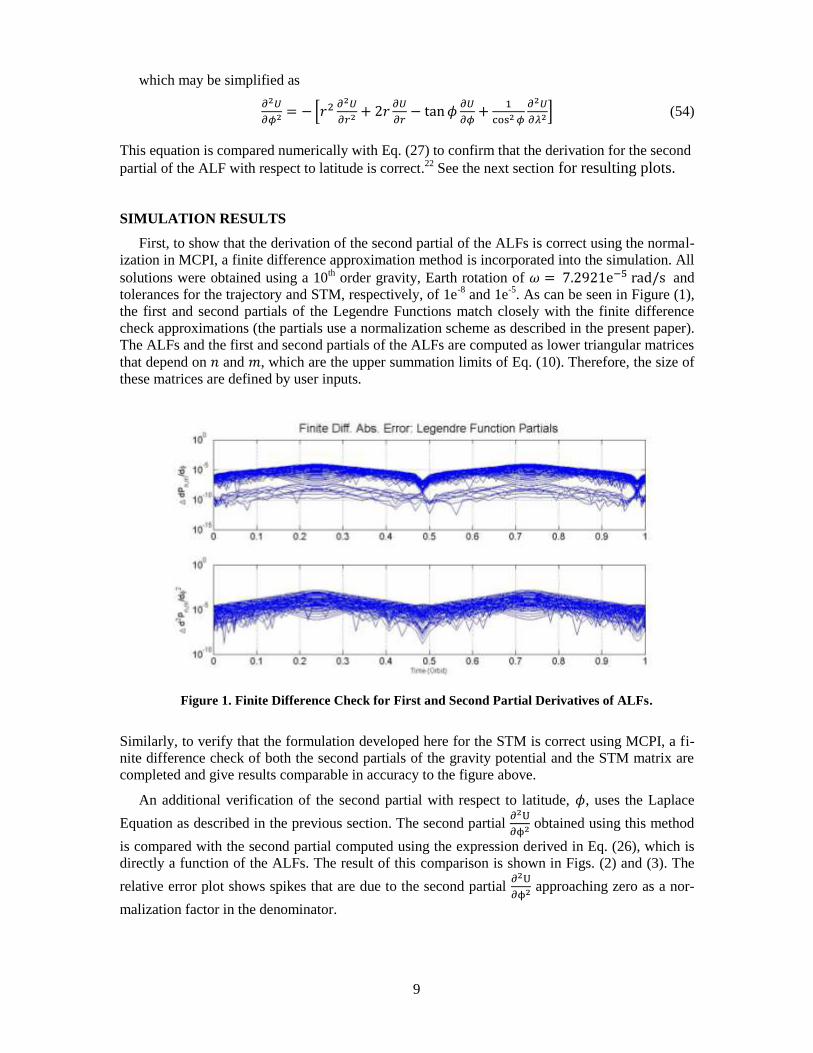
The symplectic check9 revealed an accuracy of at least for all error components, as is

seen in Figure (4). Note that each component of the 6 6 matrix of error components is plotted

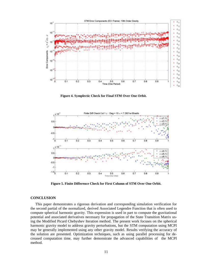
here. A final finite difference check for the STM showed that it was very accurate. Each column

of was checked using a two-sided finite difference check. The difference between the first col-

umn of the STM and the corresponding finite difference check is shown in Figure (5), though all

6 columns showed comparable accuracy for this check. The top half of Figure (5) gives the finite

difference check components on the STM's top half of the first column, while the bottom half of

the figure gives the components on the STM's bottom half of the first column.

To verify that the STM differential equation holds for arbitrary perturbations, the group prop-

erties of the STM are rigorously verified. A representative set of intermediate points are checked

using the chain rule and are satisfied with an accuracy of at least tolerance. The inverse

property of the STM is also verified to high precision.

11

Figure 4. Symplectic Check for Final STM Over One Orbit.

Figure 5. Finite Difference Check for First Column of STM Over One Orbit.

CONCLUSION

This paper demonstrates a rigorous derivation and corresponding simulation verification for

the second partial of the normalized, derived Associated Legendre Function that is often used to

compute spherical harmonic gravity. This expression is used in part to compute the gravitational

potential and associated derivatives necessary for propagation of the State Transition Matrix us-

ing the Modified Picard Chebyshev Iteration method. The present work focuses on the spherical

harmonic gravity model to address gravity perturbations, but the STM computation using MCPI

may be generally implemented using any other gravity model. Results verifying the accuracy of

the solution are presented. Optimization techniques, such as using parallel processing for de-

creased computation time, may further demonstrate the advanced capabilities of the MCPI

method.

12

ACKNOWLEDGMENTS

The sponsors for the present work are AFOSR (Julie Moses) and AFRL (Alok Das).

REFERENCES

1 Bai, Xiaoli, and Junkins, John L., "Modified Chebyhev-Picard Iteration Methods for Orbit Propagation.," Journal of

the Astronautical Sciences, Vol. 58, Issue 4, pgs. 583-613, 2011.

2 Bai, Xiaoli, "Modified chebyshev-picard iteration methods for solution of initial value and boundary value problems."

PhD Dissertation, Texas A&M University, College Station, TX, 2010.

3 Woollands, R., and Junkins, J.L., "A New Solution for the General Lambert Problem," Proceeding of 2015 AAS

GN&C Conference, Breckenridge, CO, Jan 2014.

4 Macomber, Brent, Wollands, Robyn, et. al., "Modified Chebyshev Picard Iteration for Efficient Numerical Integration

of Ordinary Differential Equations," Proceeding of 2013 AAS GN&C Conference, Breckenridge, CO, Jan 2013.

5 Kim, Donghoon, and Junkins, J.L., "Multi-Segment Adaptive Modified Chebyshev Picard Iteration Method," Pro-

ceeding of 2014 AAS/AIAA Space Flight Mechanics Conference, Santa Fe, NM, Jan 2014.

6 Woollands, R., et. al., "Validation of Accuracy and Efficiency of Long-Arc Orbit Propagation Using the Method of

Manufactured Solutions and the Round-Trip-Closure Method.," Proceeding of Advanced Maui Optical and Space Sur-

veillance Technologies Conference, Sept 2014.

7 Probe, A., et. at., "Terminal Convergence Approximation Modified Chebyshev Picard Iteration for Efficient Orbit

Propagation.," Proceedings of Advanced Maui Optical and Space Surveillance Technologies Conference, Sept 2014.

8 Battin, R., An Introduction to the Mathematics and Methods of Astrodynamics, Revised Edition, New York, NY: CRC

Press - Taylor and Francis. 1990.

9 Schaub, H., and Junkins, J.L., Analytical Mechanics of Space Systems, 2nd Edition. Reston, VA, AIAA Education

Series, 2009.

10 C.W. Clenshaw and Norton, H.J., "The Solution of Nonlinear Ordinary Differential Equations in Chebyshev Series,"

The Computer Journal, Vol. 6, 1983, pp. 88-92.

11 Feagin, T., and Nacozy, P., "Matrix Formulation of the Picard Method for Parallel Computation," Celestial Mechan-

ics and Dynamical Astronomy, Vol. 29, 1983, pp. 107-115.

12 Bai, Xiaoli, and Junkins, J.L., "Solving Initial Value Problems by the Picard-Chebyshev Method with Nvidia GPUs,"

AAS 10-197, Proceedings of 20th Spaceflight Mechanics Meeting, San Diego, CA, Feb 2010.

13 Hofmann-Wellenhof, B. and Moritz, H., Physical Geodesy, Springer-Verlag Wien, 2005.

14 Lundberg, J.B., and Schutz, B., "Recursion formulas of legendre functions for use with nonsingular geopotential

models," Journal of Guidance and Control, 11(1):31-38, Jan-Feb 1988.

15 Pines, S., "Uniform Representation of the Gravitational Potential and its Derivatives," AIAA Journal, 11:1508-1511,

1973.

16 Hobson, E., Theory of Spherical and Ellipsoidal Harmonics, Cambridge University Press, 1931.

17 Colombo, O.L., "Numerical methods for harmonic analyses on the sphere," Air Force Geophysics Laboratory; Air

Force Systems Command. 1981.

18 Rapp, R.H., "A fortran program for the computation of gravimetric quantities from high degree spherical harmonic

expansions," Reports of the Department of Geodetic Science and Surveying, Report No. 334, September 1973.

19 Gottlieb, R.G., "Fast gravity, gravity partials, normalized gravity, gravity gradient torque and magnetic field: Deriva-

tion, code, and data," Lyndon B. Johnson Space Center, February 1993.

20 Vallado, D.A., Fundamentals of Astrodynamics and Applications, 3rd Edition," Microcosm Press and Springer, 2007.

21 Kaula, W.M., Theory of Satellite Geodesy: Applications of Satellites to Geodesy, Blaisdell Publishing Company,

2000.

22 Schutz, B., Discussion of normalized associated legendre functions, Austin, TX. May 30, 2014.