Haryo Tomo

Prepocessing Aspects

of Modelling – Meteorology Basic

Air Pollution Meteorology

Atmospheric thermodynamics

Atmospheric stability

Boundary layer development

Effect of meteorology on plume dispersion

Atmosphere

Pollution cloud is interpreted by the chemical composition and physical characteristics of the atmosphere

Concentration of gases in the atmosphere varies from trace levels to very high levels

Nitrogen and oxygen are the main constituents. Some constituents such as water vapor vary in space and time.

Four major layers of earth’s atmosphere are:

Troposphere

Stratosphere

Mesosphere

Thermosphere

Atmospheric Thermodynamics

A parcel of air is defined using the state variables

Three important state variables are density, pressure and temperature

The units and dimensions for the state variables are

Density (mass/volume)

gm/cm3 ML-3

Pressure (Force/Area) N/m2 ( Pa ) ML-1T-2

Temperature o F, o R, o C, o K

T

Humidity is the fourth important variable that gives the amount of water vapor present in a sample of moist air

Equation of State

Relationship between the three state variables may be written as: f ( P, ρ ,T) = 0

For a perfect gas: P = ρ .R .T

R is Specific gas constant

R for dry air = 0.287 Joules / gm /oK

R for water vapor = 0.461 Joules / gm /oK

R for wet air is not constant and depend on mixing ratio

Processes in the Atmosphere

An air parcel follows several different paths when it moves from one point to another point in the atmosphere. These are:

Isobaric change – constant pressure

Isosteric change – constant volume

Isothermal change – constant temperature

Isentropic change – constant entropy (E)

Adiabatic Process – δQ = 0 (no heat is added or

removed )

The adiabatic law is P. αγ = constant E = T

Q

Statics of the Atmosphere

Vertical variation of the parameters = ?

Hydrostatic Equation: Pressure variation in a "motionless" atmosphere

Pressure variation in an atmosphere:

Relationship between pressure and elevation using gas law:

gz

porg

z

p

1.

2

21

dt

zd

z

pg

TR

g

z

p

p d

1

Statics of the Atmosphere

Integration of the above equation gives

Using the initial condition Z=0, P = P0

The above equation indicates that the variation of pressure depends on vertical profile of temperature.

For iso-thermal atmosphere

Therefore, pressure decreases exponentially with height at a ratio of 12.24 mb per 100m.

zTR

g

p

po

do

.exp 1

z

do

dzTR

g

p

p

0

1.ln

Lapse Rate: Lapse rate is the rate of change of temperature with

height

Lapse rate is defined as Γ = -δT δz

Value of Γ varies throughout the atmosphere

Potential Temperature: Concept of potential temperature is useful in comparing two air

parcels at same temperatures and different pressures.

Atmosphere Stability The ability of the atmosphere to enhance or to resist

atmospheric motions

Influences the vertical movement of air.

If the air parcels tend to sink back to their initial level after the lifting exerted on them stops, the atmosphere is stable.

If the air parcels tend to rise vertically on their own, even when the lifting exerted on them stops, the atmosphere is unstable.

If the air parcels tend to remain where they are after

lifting stops, the atmosphere is neutral.

Atmospheric Stability

The stability depends on the ratio of suppression to generation of turbulence

The stability at any given time will depend upon static stability ( related to change in temperature with height ), thermal turbulence ( caused by solar heating ), and mechanical turbulence (a function of wind speed and surface roughness).

Atmospheric Stability

Atmospheric stability can be determined using adiabatic lapse rate.

Γ > Γd Unstable

Γ = Γd Neutral

Γ < Γd Stable

Γ is environmental lapse rate

Γd is dry adiabatic lapse rate (10c/100m) and dT/dZ = -10c /100 m

Atmospheric Stability Classification

Schemes to define atmospheric stability are: P- G Method

P-G / NWS Method

The STAR Method

BNL Scheme

Sigma Phi Method

Sigma Omega Method

Modified Sigma Theta Method

NRC Temperature Difference Method

Wind Speed ratio (UR) Method

Radiation Index Method

AERMOD Method (Stable and Convective cases)

Pasquill-gifford Stability Categories

Surface Wind

Speed (m/s)

Daytime Insolation Nighttime cloud cover

Strong Moderate Slight Thinly overcast or

4/8 low cloud 3/8

< 2 A A - B B - -

2 - 3 A - B B C E F

3 - 5 B B - C C D E

5 - 6 C C - D D D D

> 6 C D D D D

Source: Met Monitoring Guide – Table 6.3

Sigma Theta stability classification

CATEGORY PASQUILL CLASS SIGMA THETA (ST)

EXTREME UNSTABLE A ST>=22.5

MODERATE UNSTABLE B 22.5>ST>=17.5

SLIGHTLY UNSTABLE C 17.5>ST>=12.5

NEUTRAL D 12.5>ST>=7.5

SLIGHTLY STABLE E 7.5>ST>= 3.8

MODERATE STABLE F 3.8>ST>=2.1

EXTREMELY STABLE G 2.1>ST

Source: Atmospheric Stability – Methods & Measurements (NUMUG - Oct 2003)

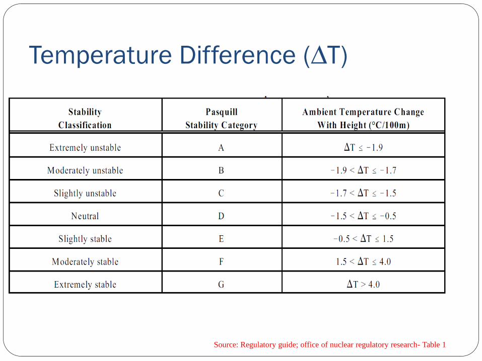
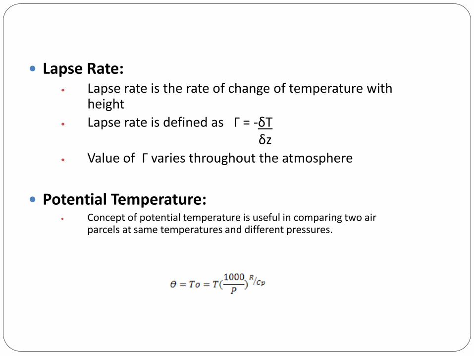
Temperature Difference (∆T)

Source: Regulatory guide; office of nuclear regulatory research- Table 1

Turbulence

Fluctuations in wind flow which have a frequency of more than 2 cycles/ hr

Types of Turbulence Mechanical Turbulence

Convective Turbulence

Clear Air Turbulence

Wake Turbulence

Boundary Layer Development

Boundary Layer Development

Thermal boundary Layer (TBL) development depends on two factors: Convectively produced turbulence

Mechanically produced turbulence

Development of TBL can be predicted by two distinct approaches: Theoretical approach

Experimental studies

Boundary Layer Development

Theoretical approach may be classified into three groups: Empirical formulae

Analytical solutions

Numerical models

One layer models

Higher order closure models

TBL using Analytical Solution

Time

Time

Time

Time

Effects of Meteorology on Plume Dispersion

Effects of Meteorology on Plume Dispersion

Dispersion of emission into atmosphere depends on various meteorological factors.

Height of thermal boundary layer is one of the important factors responsible for high ground level concentrations

At 9 AM pollutants are pulled to the ground by convective eddies

Spread of plume is restricted in vertical due to thermal boundary height at this time

Wind Velocity

A power law profile is used to describe the variation of wind speed with height in the surface boundary layer

U = U1 (Z/Z1)p Where,

U1 is the velocity at Z1 (usually 10 m)

U is the velocity at height Z.

The values of p are given in the following table.

Stability Class Rural p Urban p

Very Unstable 0.07 0.15

Neutral 0.15 0.25

Very Stable 0.55 0.30

Beaufort Scale

This scale is helpful in getting an idea on the magnitude of wind speed from real life observations

Atmospheric condition Wind speed Comments

Calm < 1mph Smoke rises vertically

Light breeze 5 mph Wind felt on face

Gentle breeze 10 mph Leaves in constant motion

Strong 25 mph Large branches in motion

Violent storm 60 mph Wide spread damage

Wind Rose Diagram (WRD)

Wind Direction (%)

Wind Speed (mph)

Wind Rose Diagram (WRD)

WRD provides the graphical summary of the

frequency distribution of wind direction and wind

speed over a period of time

Steps to develop a wind rose diagram from hourly observations

are:

Analysis for wind direction

Determination of frequency of wind in a given wind

direction

Analysis for mean wind speed

Preparation of polar diagram

Calculations for Wind Rose

% Frequency =

Number of observations * 100/Total Number of

Observations

Direction: N, NNE, ------------------------,NNW, Calm

Wind speed: Calm, 1-3, 4-6, 7-10, -----------

Determination of Maximum Mixing Height

Steps to determine the maximum mixing height for a day are:

Plot the temperature profile, if needed

Plot the maximum surface temperature for the day

on the graph for morning temperature profile

Draw dry adiabatic line from a point of maximum

surface temperature to a point where it intersects

the morning temperature profile

Read the corresponding height above ground at the

point of intersection obtained. This is the maximum

mixing height for the day

Determination of Maximum Mixing Height

Power plant Plumes in Michigan Monroe Power Plant

Power plant Plumes in Michigan

Trenton Channel

Power plant Plumes in Michigan Belle River Power Plant

River Rouge Power Plant

Photo credit: Kimberly M. Coburn