PREPARED - final report

Report06009

PREPARED - final report

VÍ-ES-06ReykjavíkMarch 2006

Ragnar Stefánsson

1 THE BACKGROUND PROBLEMS TO BE SOLVED........................................5

1.1 THE SIL-PROJECT ..........................................................................................5 1.2 THE PRENLAB-PROJECTS ............................................................................5 1.3 VARIOUS TIME SERIES OF MONITORING .............................................................6 1.4 A UNIQUE DATASET .........................................................................................6 1.5 OPPOSITION TO THE POSSIBILITIES OF EARTHQUAKE PREDICTION........................6 1.6 THE BIRTH OF THE PREPARED-PROJECT........................................................6

2 THE SCIENTIFIC/TECHNOLOGIOCAL APPROACH .....................................9

2.1 OUR APPROACH TO EARLY WARNINGS AND PREDICTIONS..................................10 2.1.1 What we aim to achieve................................................................................................. 10 2.1.2 Improving probabilistic hazard assessment .................................................................. 10 2.1.3 Time-dependent hazard assessments and warnings...................................................... 10 2.1.4 The five stages of warnings ........................................................................................... 10 Years/month in advance ......................................................................................................... 10 Weeks/days in advance........................................................................................................... 11 Hours/minutes in advance...................................................................................................... 11 The earthquake occurs ........................................................................................................... 11 Post-quake information.......................................................................................................... 11

2.2 THE SIGNIFICANCE OF ACTIVE AND WELL ORGANIZED EARLY INFORMATION AND WARNING SERVICE..............................................................................................11

3 APPLIED METHODOLOGY, SCIENTIFIC ACHIEVEMENTS AND MAIN DELIVERABLES ................................................................................................13

3.1 MODELS OF THE TWO YEAR 2000 EARTHQUAKES.............................................13 3.1.1 Earlier information and initial models.......................................................................... 13 3.1.2 The PREPARED modelling.......................................................................................... 14 3.1.2.1 The main characteristic features inferred about the June 17 earthquake.................. 16 3.1.2.2 The main characteristic features inferred about the June 21 earthquake.................. 19 Mapping of aftershocks .......................................................................................................... 19 Inversion of strong motion data ............................................................................................. 19 Inversion of geodetic data ...................................................................................................... 20 Mapping of surface rupture ................................................................................................... 20 3.1.3 About asperities in the faults......................................................................................... 21 3.1.4 Comparing the results of the different methods in studying the faulting process implies................................................................................................................................................ 23

3.2 THE MECHANICAL PROPERTIES AND THE DYNAMICS OF THE SISZ .....................24 3.3 THE RELEASE OF EARTHQUAKES ...................................................................24 3.4 TO FIND THE PLACE OF A LARGE IMPENDING EARTHQUAKE ...............................26

3.4.1 Lack of strain release in the seismic history of a fault zone, some-times called seismic gap, and sites of relatively high microearthquake activity .................................................... 26 3.4.2 Mapping of earthquake faults ...................................................................................... 28 3.4.3 Mapping of seismogenic faults with high accuracy using relative locations algorithm................................................................................................................................................ 29 3.4.4 Principal component analysis (PCA) to search for patterns in multiparameter seismic data, possibly indicating place and time................................................................................ 30 3.4.5 b-values in the SISZ to detect asperity .......................................................................... 31

3

3.4.6 Strain build-up in the South Iceland seismic zone based on GPS before the 2000 earthquakes ............................................................................................................................ 32 3.4.7 Estimation of the general rock stress tensor in the area............................................... 33 3.4.8 The SRAM method to find the probable epicenter for an impending earthquake ......... 35

3.5 WHEN WILL THE EARTHQUAKE OCCUR? OBSERVATIONS OF CRUSTAL PROCESSES LEADING TO LARGE EARTHQUAKES .......................................................................35

3.5.1 “Successful time predictions” in Iceland and the prospects........................................ 36 3.5.2 Seismicity rate expressing stress changes preceding the 2000 earth-quakes ............... 37 3.5.3 Monitoring seismicty by SAG to forecast earthquakes and eruptions ......................... 37 3.5.4 Depth variations indicating stress variations .............................................................. 38 3.5.5 Monitoring slow fault motion weeks to days before the earthquake set-off ................ 41 3.5.6 EQWA - a new short-term seismic warning algorithm ready for installation ............. 43 3.5.7 Stress changes monitored by SWS and stress relaxation ............................................. 45 3.5.8 Radon anomalies observed before the 2000 earthquakes ............................................ 47 3.5.9 Hydrological pulse observed 24 hours before the first earthquake .............................. 48 3.5.10 Earthquake triggering by another observable event ................................................... 49

3.6 IMPROVING HAZARD ASSESSMENTS AND TIME-DEPENDENT ASSESSMENTS OF PROBABLE EARTHQUAKE EFFECTS........................................................................50

3.6.1 Some results of PREPARED that will help in enhancing the hazard assessments........ 51 3.6.1.1 The significance of the new modelling ...................................................................... 51 3.6.1.2 To identify the dangerous fault................................................................................... 51 3.6.1.3 Slip inversion models ................................................................................................. 52 3.6.1.4 From “classical” hazard assessment to dynamic hazard assessments...................... 52 3.6.1.5 Attenuation of strong ground motion and site effects................................................. 52

3.7 THE EARLY WARNING AND INFORMATION SYSTEM OF ICELAND (EWIS)............53 3.8 ADVANCES IN PROVIDING EARLY INFORMATION AND WARNINGS ABOUT EARTH-QUAKES .............................................................................................................54

3.8.1 The PREPARED-project results in manyfold progress towards mitigating risks in this way ......................................................................................................................................... 55 3.8.2 Short-term alerts .......................................................................................................... 55

3.9 FUTURE RESEARCH TOWARDS A FURTHER PROGRESS IN EARTHQUAKE WARNINGS.........................................................................................................................55

4 CONCLUSIONS INCLUDING SOCIO-ECONOMIC RELEVANCE, STRATEGIC ASPECTS AND POLICY IMPLICATIONS....................................57

5 DISSEMINATION AND EXPLOITATION OF THE RESULT..........................59

REFERENCES ...................................................................................................61

4

1 The background problems to be solved Through the history of Iceland earthquakes are known to have caused much destruction, especially in the South Iceland seismic zone and along the north coast of Iceland. Many times this was a striking fear in the community. During the later part of the 20th century the fear for repeated such activity led to several actions of preparedness including multipurpose real-time monitoring of the area. Scientific researchers undertook hazard assessments to prepare for stronger building codes, as well as carrying out studies to try to understand the dynamics. Like in any other earthquake-prone country there has been a strong wish to foresee such hazards, and it has been a challenge for scientists. In the early 1980’s the Council of Europe decided to strengthen earthquake prediction research in the European areas. For this reason it allocated a few test zones, areas of strong earthquakes, for multinational efforts in this field. The South Iceland lowland was allocated as such a test area. The South Iceland seismic zone (SISZ), with its history of hazardous earthquakes, goes from east to west through this fruitful farming area of Iceland. The Nordic countries, Iceland and Scandinavia, took this challenge and since 1988, Iceland and especially the South Iceland lowland, has been a European test area for earthquake prediction research. The basis for the creation of this test area, and of its usefulness, is high earth activity, various favourable natural conditions and the build-up of high-level geophysical monitoring systems, as well as the build-up of high-level scientific capabilities. The PREPARED-project is strongly related to and based on the achievements of the earlier multinational projects. Therefore they are listed here. 1.1 The SIL-project “Earthquake prediction research in the South Iceland lowland” (1988-1995), was a common project of the Nordic countries. Its main achievement was to develop and install the SIL seismological measurement system around the SISZ, revealing detailed information about crustal conditions and crustal processes based on microearthquakes. It was assumed that microearthquakes down to magnitude zero would give us the best information in time and space about the physics of crustal processes leading to large earthquakes. The high-level automatic acquisition and evaluation procedures were also a basis for short-term alerts and warnings, ahead of earthquakes and volcanic eruptions. 1.2 The PRENLAB-projects ”Earthquake prediction research in a natural laboratory.” These were the European Commission seismic risk projects, PRENLAB and PRENLAB-2, carried out in 1996-2000. These were multidisciplinary research projects aiming at better understanding of processes leading to large earthquakes and their effects. Multidisciplinary approach of geoscientists was needed to interprete the huge new information about crustal processes

5

which the SIL-system carried to the surface. Geologists, geophysicists, geodetists and theoretical modellers joined in at the test site. The PRENLAB-projects involved much basic research work, which was needed, but linked to their acitvities was also the initiation of continuous real-time GPS measurements in Iceland and in general increased geophysical monitoring. Intensive geological field studies to increase the basic data. Historical studies and paleoseismic studies were carried out to extend the basic data farther back in time. 1.3 Various time series of monitoring In addition to SIL various time series of monitoring were intensified because increased expectations for large earthquakes in the SISZ. Repeated GPS measurements began in the area before 1990, becoming continuous in 1998. Volumetric borehole strainmeter measurements started in the SISZ in 1979. Time series of radon exist from 1977 to 1993 and since 1999. A network of strong-motion seismometers recorded the earthquakes in 2000. Renewed geological studies revealed faults and soil structure. 1.4 A unique dataset The intensive monitoring aimed for earthquake prediction research collected a unique dataset. For the year 2000 earthquakes, it reveals premonitory process, nucleation, fault process and co-seismic effects as well as long-lasting and wide-spread triggered activity. Studying these data provides an opportunity to understand the crustal processes involved in and preceding earthquake release and they are a basis for warnings. 1.5 Opposition to the possibilities of earthquake prediction Near the start of the SIL-project opposition against the possibilities of earthquake prediction intensified. It was claimed by some high ranked scientists around the world that earthquake prediction was impossible and that it would never be possible. This for a while lowered the position of earthquake prediction research in the scientific world. These critical ideas were based on some earlier misfortunes in earthquake prediction. They influenced the research efforts in the in SIL test area in such a way to put more efforts to the physical and multidisciplinary approach rather than to the pattern search in seismic catalogues only, as had been characterizing earlier earthquake prediction efforts. 1.6 The birth of the PREPARED-project The South Iceland seismic zone was the main test area for the projects described above. Therefore it was like a test for the success of the research and monitoring efforts when two Ms=6.6 earthquakes struck South Iceland in June 2000. The warnings and information which were issued showed the significance of the earthquake prediction research. The data which were collected were significant for further research and better warnings and information service in the future. This put the PREPARED-project on the agenda. It has been a special objective of the PREPARED-project to make use of the valuable observations that were made before, during and after these earthquakes, to

6

develop methods and understanding for better hazard assessments and warnings in the future. This was done through multidisciplinary, multinational scientific approach. The project continued and proceeded from the basic results of the earlier earthquake prediction research projects towards application for direct long-term and short-term warnings. PREPARED was aimed at preparedness towards earthquake hazards and to mitigate seismic risk. It aimed towards developing technology to assess what earthquake effects may occur and where. It aimed to use observed end expected earthquake forerunners and crustal changes to develop methods for earthquake warnings on a long-term and short-term basis. By fast evaluation of the impacts of earthquake hazard, before or after its onset, it helps to prepare necessary and effective rescue actions. It developed close relationship with an early warning and information system (EWIS) and with the Civil Defence of Iceland, and the test area for PREPARED, for testing and application of its methods. The objective was to develop methodology which can be applied to mitigate risks anywhere. Understanding what ground motions can be expected at various places in populated areas is socially and economically significant. To understand where the faults rupture the surface and when, is of huge significance in any earthquake-prone country.

7

2 The scientific/technologiocal approach Two magnitude Ms=6.6 earthquakes rocked the inhabitants of the South Iceland seismic zone (SISZ) in June 2000 for the first time, so severely, in almost a century. Previous to the 2000 events, the last sequence of six such large earthquakes in this zone occurred in the period 1896-1912. Their magnitude reached 7, as recorded instrumentally for the 1912 earthquake. Observations of these two earthquakes, and earlier observations in the SISZ as well as scientific findings of earlier research were the scientific input in the project (Figure 1).

Figure 1. Earthquakes in SISZ since 1700. The earthquakes arrange side by side each having right-lateral slip on a NS fault. The fault epicenters and magnitudes (Stefánsson et al. 1993; Clifton and Einarsson 2005; WP4.3 of the Third Periodic Report) are estimated from historical data and the fault lengths are from Roth (2004). The main anticipated results of the project were methodology and alert procedures that can be applied for enhanced hazard assessment and for issuing information and warnings which are significant for mitigating seismic risk. The dissemination of the scientific results was intended to be through the Icelandic early warning system (EWIS at IMO) to the civil defence infrastructure of Iceland and to other scientists at conferences and through open reports and peer-reviewed journals. The results are of course especially well distributed and qualified in discussions by the participants in the project which come from 8 European countries.

9

2.1 Our approach to early warnings and predictions

2.1.1 What we aim to achieve The role of earth sciences in mitigating seismic risk is manifold. We try to provide (time-independent) probabilistic hazard assessment, time-dependent hazard assessment, short-term warnings and early warnings or “nowcasting”. “Nowcasting” means to provide basic information about an earthquake that has occurred for mitigating its risk effects. Nowcasting is included in all prewarning procedures. But for nowcasting it is significant to know as much as possible ahead of the striking earthquake. The basic purpose of all these information or warnings is to assess as well as possible and as early as possible the exact location and surface effects of the impending earthquake.

2.1.2 Improving probabilistic hazard assessment On basis of earlier studies, by precise mapping of numerous activated faults, by various observed surface effects and by modelling with earth-realistic parameters, we have aimed to make the hazard assessment more detailed as concerns the place and effects. This involves to forecast ground motion for preventive actions and engineering application.

2.1.3 Time-dependent hazard assessments and warnings Earthquake prediction informing with useful precision about all aspects of an impending earthquake is hardly on the agenda for the time being. Therefore our approach to prediction is a gradual approach, enhanced with gradual increase of our understanding of crustal processes. Based on our experience it is possible in many cases to provide useful information at different times in advance about some aspects of a probably impending earthquake and gradually closing in on the expected event with increased research and monitoring. Judging from experience and availability of tools in Iceland, we based our approach on real-time information of microearthquakes and larger earthquakes, on hydrological data, radon anomalies, strain/deformation observations, as well as earth-realistic models of crustal behavior and processes. We based it on careful watching and real-time research in each stage of the development of premonitory earthquake signals.

2.1.4 The five stages of warnings In the PREPARED approach we classified our earthquake warnings and time-dependent hazard assessments into several scenarios or stages:

Years/month in advance Useful for concentration of various risk mitigating efforts, finding baseline, increasing research, increasing monitoring and strengthening of structures.

10

Weeks/days in advance Useful for activating the civil protection and rescue groups, increased earth observations, and raising preparedness of people.

Hours/minutes in advance Everyone involved begins preparing immediately for a hazardous event that will occur anytime shortly. Such an alarm must have time limit; it must end sometime.

The earthquake occurs Early warning, nowcasting, real-time damage assessment. Usefulness: Assessment based on earlier knowledge as well as from observations of the earthquake used to help people and authorities, civil defence and rescue groups to mitigate the impact on people and society.

Post-quake information To explain the hazardous event and try to assess and warn of further coupled hazards. The aim of the project is to apply the available knowledge and results of earlier research and the new data acquired to enhance the understanding as well as information and warnings given at all these stages. The various workpackages of the project will aim at concrete results to enhance general hazard assessments, time-dependent hazard assessments, short-term warnings and nowcasting (early information) for an impending earthquake. Although this is in first hand valid for mitigating risk in Iceland, the multidisciplinary and physical approach makes the results applicable at many other earthquake-prone regions of the world. 2.2 The significance of active and well organized early information and warning service Earthquake prediction research is in a state of development. Although we can by no means claim that it is possible to warn against all earthquakes, we concluded that results of multidisciplinary earthquake prediction research are already providing answers which help to provide warnings about some aspects of impending earthquakes in some cases. A good example of this is a very useful warning that was issued to the Civil Defence of Iceland 25 hours before the second magnitude 6.6 earthquake in South Iceland struck on June 21, 2000. In this warning the correct location was stated within a few kilometers, as well as the right fault orientation and magnitude for the earthquake. The warning urged the civil defence organizations to take all necessary preparatory measures for an earthquake that should be expected at any moment.

11

There was no short-term warning before the first large earthquake of year 2000, i.e. on June 17. However, there was a general assessment, published in journals, about the probable location (and the fault direction) of the next expected large earthquake in SISZ. The June 17 earthquake occurred within the 5 km wide area of expected location. In hindsight studies it was observed that even the first earthquake had small foreshocks that could have been useful for short-term warning if the information which they carried would have been detected early enough (Stefánsson et al. 2003; Stefánsson and Guðmundsson 2005a). In research within the PRENLAB-projects it was revealed that all larger earthquakes (M>4.5) in the previous 10 years in Iceland had been preceded by small premonitory activity, indicating that in these earthquakes, related processes started before them (Slunga 2003). In 1998 a magnitude 5 earthquake was forecast to be imminent at the western end of the SISZ. The prediction, size and location, was made a few days ahead of the event, in real-time, on basis of shear-wave splitting time, on basis of high nearby seismicity and in general on basis of understanding of the tectonics of the area (Crampin et al. 1999). It is a request from society and from the scientific community to find ways to understand and make use of such possible premonitory effects for warnings, short- or long-term, if possible. On basis of increasingly good prospects for being able to provide useful warnings ahead of earthquakes IMO started the development of an early information and warning system (EWIS) with support from the Icelandic government. The aim was to merge together real-time observations to be able to access old knowledge quicker as well as evaluation tools that could serve the scientists in real-time research. Good tools for fast evaluations and algorithms that can serve real-time research is essential in such a gradual approach to prediction as is aimed at in the PREPARED-project. We cannot rely on that earthquakes will repeat the behaviour of old earthquakes or on models that we have tried to create in order to simulate future earthquakes. The closer in time that we come to the earthquake release the better possibilites we have to foresee the process. That is the idea behind the stepwise approach which is outlined above. We will learn during the preparatory and nucleation process. For that we need tools that can evaluate observations quickly, to visualize them, to model them better, and to prepare safer warnings.

12

3 Applied methodology, scientific achievements and main deliverables The methodology applied is multidisciplinary, reflecting the multidisciplinary character of the approach. I will here describe shortly some main achievements and refer to papers and reports for the details. I will divide it into chapters about the type of achievements reached. Observations come before modelling. Still I will begin with the main modelling results and after that describe the methods and observations that are applied in warning service. The reason for this is that the models are new, they have been created within this project and the former earthquake prediction research projects in Iceland. They have been created interactively between the observations and the theoretical work. So we begin with describing shortly the main results achieved in modelling and use them for interpreting the observations and explain how the observations imply methods for time-dependent earthquake hazard assessments and earthquake warnings. 3.1 Models of the two year 2000 earthquakes

3.1.1 Earlier information and initial models The focal mechanism based on teleseismic observations of the two magnitude 6.6(Ms) earthquakes was studied by several agencies. Harvard centroid moment tensor evaluation gave the following results: For the first earthquake: Date: 2000/6/17 Centroid Time: 15:40:50.7 GMT Lat=63.99 Lon=-20.47 Depth=15.0 Half duration=4.4 Centroid time minus hypocenter time: 9.0 Moment Tensor: Expo=25 -0.935 1.189 -0.254 -0.156 -1.922 6.730 Mw=6.5 mb=5.7 Ms=6.6 Scalar Moment=7.05e+25 Fault plane: strike=273 dip=74 slip=-3 Fault plane: strike=4 dip=87 slip=-164

13

http://pubweb.parc.xerox.com/map/color=1/lat=63.99/lon=-20.47/mark=63.99,-20.47

For the second earthquake: Date: 2000/6/21 Centroid Time: 0:51:54.8 GMT Lat=63.98 Lon=-20.85 Depth=15.0 Half duration=4.2 Centroid time minus hypocenter time: 7.9 Moment Tensor: Expo=25 -0.746 0.595 0.151 0.199 -1.136 5.301 Mw=6.4 mb=6.1 Ms=6.6 Scalar Moment=5.44e+25 Fault plane: strike=271 dip=77 slip=-5 Fault plane: strike=2 dip=85 slip=-167 According to the database of the Icelandic Meteorological Office (IMO) the origin time of the June 17 earthquake was 15:40:40.94 GMT, the hypocenter at 63.97 N, 20.37 W, and a hypocentral depth of 6.3 km. First evaluation of aftershocks indicated an 11-12 km long rupture extending from the surface to 10 km depth. Assuming that the upper 1 km of the rupture does not contain considerable energy to be released in the earthquake the fault width is taken to be 9 km. The aftershocks indicated that the fault strikes N7 E and dips 86 towards the east (Stefánsson et al. 2003). The IMO determined origin time of the June 21 earthquake was 00:51:46.95 GMT, the hypocenter was at 63.98 N, 20.71 W, and a hypocentral depth of 5.1 km. The aftershocks indicate a vertical fault, 15 km long, striking N2 W extending from the surface to 8 km depth (Stefánsson et al. 2003). From geological considerations and general understanding of the tectonics, the right lateral slip on NS faults was stated in both cases.

3.1.2 The PREPARED modelling Within the PREPARED-project detailed slip models for the June 17 and June 21 main shocks have been estimated from a joint inversion of InSAR and GPS data (Pedersen et al. 2003) and strong motion data (Suhadolc and Sandron 2005). The sub-surface fault structures of the two events have also been mapped by relative relocations of aftershocks (Hjaltadóttir and Vogfjörð 2005) and the surface fractures in the two epicentral areas have been mapped (Clifton and Einarsson 2005). The following is a summary of the main results from the workpackages and a comparison of the models (Hjaltadóttir et al. 2005). Figure 2 shows vertical cross-sections of the faults of the two earthquakes and the inferred slips. Figures 3 and 4 show in surface view the distribution of aftershocks following the earthquakes and the geologically inferred surface fissures.

14

http://pubweb.parc.xerox.com/map/color=1/lat=63.98/lon=-20.85/mark=63.98,-20.85

Figure 2. Left: The June 17 fault. Right: The June 21 fault. Top: Relatively located aftershock distribution on the fault planes in a vertical view from east. Middle: Right-lateral fault slip models for the June 17 and June 21 main shocks derived from joint inversion of InSAR and GPS data. The size of each grid cell is 1.5•1.5 km. Bottom: Slip distribution obtained from strong motion data. The value for each grid cell is plotted in a discrete coloured scale of intensities. The size of each grid cell is 2•2 km. The stars show the main shock hypocenter locations.

15

3.1.2.1 The main characteristic features inferred about the June 17 earthquake Mapping of aftershocks Mapping of aftershocks indicates that the fault is roughly 12.5 km long and 10 km deep. Aftershocks on the fault are mainly confined to the fault margins, mostly below 3 km, and a cluster in the center of the fault, around the hypocenter (Figure 2). During the first 24 hours, however, aftershocks were distributed over the entire fault. The fault is near vertical, the overall strike is ~7°, but it is composed of many smaller sections with differing strikes. Above 8 km depth the aftershocks display a rather discontinuous pattern composed of three main patches, each approximately 2-3.5 km long (Figure 3). The central patch is very planar and is active throughout the year. Its strike (~11 degrees) is slightly east of the overall strike of the fault. Activity on the northernmost fault section is mostly near its northern edge, where it branches into a few short N-striking patches. The southernmost section is more continuous and bends westwards with decreasing latitude. At the southern tip the fault jumps half a kilometer to the west and continues on a ~2 km long segment. West of the southern edge, a few small faults were also activated. Their strikes are generally west of north. Below 8 km depth the aftershocks define a continuous fault trace, but with kinks at the intersections of the main sections above. Below the northernmost fault section, the bottom appears to be composed of a few smaller en-echelon faults and then breaks up into separate parallel branches farther north. Activity on the southernmost fault patch, on the other hand, appears to be continuous and more linear, bending slightly westward towards the southern end (Hjaltadóttir and Vogfjörð 2005; WP 4.1 of the Third Periodic Report). Inversion of strong motion data Strong motion data is inverted for distribution of seismic moment on the fault, with total moment constrained by the observed teleseismic moment. The results calculated on a grid with 2 km resolution, show that most of the moment is released on the central patch, with a peak below the hypocenter, extending ~8 km northwards along the fault and down to ~8 km depth near the center. A second maximum is located at shallow depth (3 km) roughly 6 km south of the hypocenter. Two additional peaks in momentum are also obtained near the surface (1 km depth), one at the northern margin of the fault and the other above the hypocenter. In Figure 2 seismic moment is converted to displacement using a constant shear modulus. If account is taken of the increase in velocity with depth (increasing shear modulus with depth), displacement at the surface increases significantly which is questionable (WP 4.2 of the Third Periodic Report). Inversion of geodetic data Inversion of GPS and InSAR data for slip on the fault, in 1.5 km cells, shows the displacement approximately covers the aftershock region, but slip is greatest above and south of the hypocenter. Maximum slip is attained between 3 and 4 km depth, roughly 2

16

km south of the hypocenter, which is both shallower and south of the maximum obtained from the strong motion inversion (Pedersen et al. 2003; WP 4.4 of the Third Periodic Report). Mapping of surface rupture Mapped surface rupture shows a discontinuous pattern distributed asymmetrically along the fault defined by the relocated event distribution. Most surface ruptures occur along NNE-striking left-stepping en-echelon segments within a 2 km wide zone, approximately centered on the fault, though the majority occurs on the western edge (Figure 3). When compared to the geodetic and strong motion results, the distribution and intensity of surface rupture agrees well with the geodetic maximum slip, south of the hypocenter, and with the maximum moment, just below the hypocenter. There, a 2.5 km long continuous fracture was observed, west of the event distribution on the center fault patch. Another 3 km long segment extends northwards approximately 1 km west of the fault, but the northernmost segments lie approximately parallel above and just east of the event distribution, which also shows fracture on parallel segments at depth. To the south, the surface ruptures fall just east of and along the southernmost patch (Clifton and Einarsson 2005; WP4.3 of the Third Periodic Report).

17

Figure 3. The aftershocks and surface ruptures on the Holt fault, i.e. the first earthquake, June 17, 2000. The hypocenter of the Ms=6.6. earthquake is denoted with a star. A hypocenter for a smaller earthquake occuring roughly 2 minutes later, is also marked by a smaller star. All events are shown in the background in grey. Events on identified faults are displayed in colour, according to age (from June 17 to December 31) and for different depth ranges. Yellow lines display surface rupture from 2000, brown segments are older fissures.

18

3.1.2.2 The main characteristic features inferred about the June 21 earthquake

Mapping of aftershocks During the time period between the two main shocks (June 17 to 21), seismic activity in the epicentral area of the June 21 fault was mainly along the bottom of the eventual fault and along the trace of the mapped conjugate surface faults at ~63.95°N, extending westward from the main fault. During the first 24 hours following the June 21 event, the aftershocks, however, were distributed over the entire main fault up to about 1 km depth. After that, activity concentrated along the bottom, except at the southern end, where it was distributed over the whole depth range and continued throughout the year. South of the hypocenter, aftershocks are evenly distributed over the fault, while north of the hypocenter the activity is sparser and mostly concentrated near the bottom. The overall fault length, defined by the aftershocks, is 16.5 km and its strike is 179°. The fault depth increases southward, from ~7 km on the northern half to ~10 km at the southern margin (see Figure 2). Near the hypocenter the fault branches into two faults with different dips. The southern half is vertical and extends north to 64°N, terminating at the southern shore of lake Hestvatn. The northern half dips 77°E and extends from the hypocenter to the northern margin of the fault (64.05°N). Both branches continue with a similar northerly strike and follow approximately the same trace at the bottom, creating an approximately 3 km long wedge north of the hypocenter. The intersection of the dipping segment with the surface, approximately matches the mapped surface ruptures west of lake Hestvatn. At the southern terminus, the fault is broken up into many small fault segments of 1-2 km diameter and with varying strike. Near the location of the mapped conjugate surface rupture (Figure 3), the earthquake distribution is denser and extends westward, mostly on short easterly striking segments. About 3 km farther south, a second set of conjugate faults, extending over a wide depth range (2-9 km) is also defined by the seismicity (Hjaltadóttir and Vogfjörð 2005; WP4.1 of the Third Periodic Report).

Inversion of strong motion data Inversion of strong motion data for moment distribution on the fault shows that the maximum in moment release is located at a depth of 5 km, ~1 km south of the hypocenter, which is also at the intersection with the westward extending conjugate fault (where surface rupture was observed). An increase in moment release follows approximately the distribution of aftershocks along the bottom of the fault, increasing in depth from 7 km on the northern half of the fault to 11 km just south of the hypocenter. Two additional maxima are located just below the surface. The smaller one is 3 km south of the hypocenter, the other is 3 km north of the hypocenter, approximately at the end of the vertical section of the fault. Strike of the fault was assumed 358° and the dip is 90° similar to what was found from the aftershock distribution (WP4.2 of the Third Periodic Report).

19

Inversion of geodetic data Inversion of GPS and InSAR data for slip on the fault shows the displacement approximately covers the aftershock region. The maximum depth of 10 km is attained in the south center of the fault. Maximum slip is obtained above the hypocenter, at approximately 4 km depth, 3-4 km north of the hypocenter. This does not agree with the strong motion results. However, the dipping northern fault segment defined by the aftershocks, could account for the apparent increased slip north of the hypocenter, since the geodetic solution allows only constant dip on the whole fault. The smaller peak in slip, obtained at the same depth and 1-3 km south of the hypocenter agrees rather well with the strong motion results. The geodetic data record the co-seismic deformation as well as any rapid transient motion that occurred during the data acquisition (~2 weeks for the GPS, ~1 month for the InSAR). This may explain some differences in the distributed slip models obtained from the geodetic and strong motion data (Pedersen et al. 2003; WP4.4 of the Third Periodic Report).

Mapping of surface rupture Mapped surface rupture (Figure 4) shows a discontinuous pattern distributed asymmetrically along the fault defined by the relocated event distribution. The pattern is more complex than for the June 17 fault. At the southern end of the fault, where the clustering of aftershocks is the densest, no surface rupture has been observed, but 2-3 km farther north, a NNE-trending segment lies west of the fault, almost in continuation of the largest left-lateral conjugate fault, mapped at depth (Figure 2). Another NNE-trending segment of similar length is observed, where the large conjugate fault extends from the fault to the west, 2.5-3 km south of the hypocenter. It is 2.5 km long and is by far the longest EW-trending segment observed in the SISZ and shows a left-lateral strike-slip motion. This segment is not clearly seen by the relocated event distribution, but there is an indication of a fault, extending ~1 km to the SW from the main fault. The results from the strong motion data show a small maximum just below the surface at the location of the conjugate fault. No surface rupture has been observed above the epicenter, but 1.5-2 km further north, segments are mapped well west of the linear event distribution, approximately where the 77° dipping fault intersects the surface (Clifton and Einarsson 2005; WP 4.3 of the Third Periodic Report).

20

Figure 4. The aftershocks and surface ruptures on the Hestvatn fault. The hypocenter of the June 21, M=6.6 (Ms) earthquake is denoted by a star. All events are shown in the background in grey. Events on identified faults are displayed in colour, according to age (from June 21 to December 31) and for different depth ranges. Yellow lines display surface rupture from 2000. The brown line segments denote older fissures.

3.1.3 About asperities in the faults It has been claimed that the central area of the June 17 earthquake fault, i.e. the area of high microseismicity in Figure 2, is an asperity, a hard core, and the breaking of it where the hypocenter is, was the nucleus of the earthquake (Stefánsson et al. 2003). Its center has been put to 6 km depth and the diameter to 3 km. The existence of such an asperity also explains some patterns in the pre-earthquake activity (Stefánsson and Guðmundsson 2005a).

21

The last phase in the earthquake nucleation process (the breaking of the asperity) is comparable to a magnitude 5-5.5 according to seismic measurements. This is well recorded in the strainmeters data from the vicinity of the earthquake epicenter. Figure 5 shows the nucleation signal recorded with a strainmeter at Skálholt (SKA), at 20 km distance from the epicenter. The first two seconds of the record show a signal before the real onset of the fault starts. The second triggered earthquake, the June 21 one, did not have such an asperity signal, and thus not a developed asperity as the first one.

Figure 5. A strainmeter record from SKA, 20 km to the west of the June 17 earthquake. It shows a nucleation phase 1.8 seconds before motions starts on the fault plane as a whole. Aftershocks continue in the asperity area after the earthquake in the same way as at the fault boundaries, at the bottom as well as at both ends of the fault, indicating the same direction of slip as in the earthquake. Thus some strength was left in the asperity after the earthquake at least more strength than in the surrounding fault plane. The stress was not totally released in the asperity during the earthquake, compared to the surrounding part of the cross-section. The second triggered earthquake, the June 21 one, did not have such an asperity signal in the seismic or strainmeter records, and thus not a developed asperity as the first one. The aftershocks do not cluster in the hypocentral area as in the first earthquake although the hypocenter was in the central part of the fault. The second earthquake was triggered by the first which had strong enough coseismic strain effect at the southern end of the 21 June fault to trigger a start of a slow earthquake slip there (Árnadóttir et al. 2003). Slow slip before the 21 June earthquake is expressed in high microearthquake density mainly below the hypocenter at 6-7 km depth, and along a conjugate fault 2-3 km to the south of the hypocenter (Hjaltadóttir and Vogfjörð 2005). The nucleation of the second earthquake started by swarm activity and fluid intrusion in a junction between the NS fault and WSW conjugate fault immediately after the first

22

earthquake. This pre-earthquake period strained the area a couple of kilometers to the north, where the hypocenter is as well as the fault plane to the south. Homogenization of the stress field along the becoming fault took place through fluid migration along it at depth during the days from the first earthquake, making slip possible across the whole fault plane (Stefánsson and Guðmundsson 2005a).

3.1.4 Comparing the results of the different methods in studying the faulting process implies There is a difference in slips from the deformation measurements and the strong motion inversions (Hjaltadóttir et al. 2005) which may be possible to explain why the strong motion inversions express the immediate earthquake slip, while the geodetic measurements take to a longer time interval between measurements. The aftershocks and the strong motion inversion reflect the breaking of an asperity in the first earthquake and the breaking of a barrier towards the south of it in the second large earthquake. Both the strong motion inversion and the deformation modelling show little slip below the hypocenter depth, i.e. below 7-8 km, supporting the suggestion that slow earthquake slip started at depth before the earthquakes. All the 3 methods imply directly or indirectly shallowing of the 21 June seismogenic zone to the north (Hjaltadóttir et al. 2005). The reason for this may be that this fault stood for a long-time in a stress shadow of the first earthquake asperity, but maybe more significantly the northern part was in stress shadow of the central to southern part of the fault. Upward migrating fluids corroded the deeper parts of the fault to the north. That might explain much slip inferred from deformation, but little slip inferred from strong motion. There is much work left in comparing the different kind of observations around the two major earthquake faults. Such work is significant because it will probably bring us closer to being able to understand the earthquake process. The work is of course hampered by the lack of continuous GPS-stations around the faults and also by how few seismic strong motion instruments were available around the faults at the moment of the earthquakes. Further readings Bergerat, F., J. Angelier, Á. Guðmundsson & H. Torfason 2003. Push-ups, fracture patterns, and paleoseismology of the Leirubakki Fault, South Iceland. Journ. Struct. Geol. 25, 591-609. Geirsson, H., Þ. Árnadóttir, C. Völksen, W. Jiang, E. Sturkell, T. Villemin, P. Einarsson, F. Sigmundsson & R. Stefánsson 2005. Current plate movements across the Mid-Atlantic Ridge determined from 5 years of continuous GPS measurements in Iceland. J. Geophys. Res. Accepted. LaFemina, P.C., T.H. Dixon, R. Malservisi, Þ. Árnadóttir, E. Sturkell, F.Sigmundsson & P. Einarsson 2005. Geodetic GPS-measurements in South Iceland: Strain accumulation and partioning in a propagating ridge system. J. Geophys. Res. In press.

23

Pagli, C., R. Pedersen, F. Sigmundsson & K.L. Feigl 2003. Triggered fault slip on June 17, 2000 on the Reykjanes Peninsula, SW Iceland, captured by radar interferometry. Geophys. Res. Lett. 30(6), 1273. 3.2 The mechanical properties and the dynamics of the SISZ An innovative outcome of modelling work within PREPARED, is that high pore pressure values can efficiently migrate from below the brittle-ductile transition to shallower. This model is based on earth-realistic parameters for the area and supported by various observations in the SISZ (WP6.2 of the Third Periodic Report; Zencher et al. 2005). A general feature of the SISZ is stable motion at depth and corresponding stable build-up of strain in a 10-15 km broad EW zone in the upper brittle part of the crust. This EW zone is a weak zone compared to the surrroundings, penetrated from below by fluids with high pressures. The shearing strain in the zone is a result of continuous EW plate motion variably loaded by the nearby volcanic activity and the activity of the adjacent rifts and hotspot/plume (Stefánsson et al. 2005). Further readings Antonioli, A., M.E. Belardinelli & M. Cocco 2004. Modelling dynamic stress changes caused by an extended rupture in an elastic stratified half-space. Geophys. Journ. Int. 157(1), 229-244. Bonafede, M. & E. Rivalta 2005. Crack models of faults and dikes in layered visco-elastic media. In preparation. 3.3 The release of earthquakes Comparing historical earthquakes with recently observed microearthquakes (Stefánsson and Guðmundsson 2005a) and modelling (Stefánsson et al. 2005) reveals the following process for the relase of large earthquakes in the SISZ: Ongoing all the time is stable motion at depth. Fluids are continuously, slowly, released from the ductile deeper part of the crust, near the brittle/ductile boundary. The stable motion is disturbed at times with earthquakes, unstable process: Step 1) An old fault is (mostly) seismically dormant for a few to several hundred years. It was near totally released in an earthquake a few hundred years ago, both as concerns tectonic shearing as well as pore pressures. Step 2) After some time, time length both based on the strain rate and availability fluids, fluids carrying lithostatic pressures start to penetrate up into the damage zone of the brittle crust as cracks open, carrying high fluid pressures from below and gradually creating higher pore pressures at shallow depths in the crust. Medium size earthquakes occur at some parts of the fault, but the slip does not proceed along the whole fault while stress around the fault is heterogeneous. The fault as a whole is not ready to slip. It creates volumes in the crust where minor seismic swarms are frequent, related to the

24

upstream of the fluids, assumed to be mostly water. The heteorogeneity of the fault area opens the gates for local upflow of fluids, and the local stress conditions are modified by fluid/rock corrosion and strain around the fault. Gradually the fault is corroded by the fluids to such a degree that an asperity is left which the fluids pass by. The existence of the strong core heterogeneity controls locally the crustal response to the regional strain. Figure 6 from Stefánsson and Guðmundsson (2005a) is a schematic description of some observed features before the June 17 earthquake in a 10•10 km area around the fault.

Figure 6. Schematic picture of the conditions around the June 17 earthquake before its occurrence in the framework of the SISZ. The EW motion across the SISZ is shown by left-lateral arrows, and the boundaries of the 10 km SISZ is shown with blue lines. The June 17 fault (red) has a strike of 7ºNE. The 3 km diameter asperity is shown in dark grey. The regional horizontal stress axes are shown by arrows, and the maximum horizontal compression is here taken as 50ºNE. The local field heterogeneity caused by the left-lateral steady motion across the hard core is indicated by opposite short arrows. The areas of the premonitory swarm activity for decades, the “dilavolume” is in light grey (left figure). The line segments indicate frequent fault planes. The right figure describes the last 17 days before the earthquake. The microearthquakes now cluster near the fault plane and mostly below 6 km, with fault planes en-echelon in accordance with the right-lateral motion which has started at depth (Stefánsson and Guðmundsson 2005a; Stefánsson et al. 2005). Step 3) Initiation at depth of fault movement along an old NS fault, accompanied and pushed by fluids streaming into the fault. The fluids causing overpressures in the swarm activity volumes (dilavolumes) shift to the fault area, which has a better direction to release the plate motion strain. The fault motion, which starts down in the ductile part, and the normal faulting part between say 7-13 km propagates horizontally along the fault plane and gradually also upward, as well as fluids which help to lower the normal pressure on the fault. A weakness in the fault finally shows up by accelerated motion of

25

the fault plane as a whole, shown by small earthquakes all over the fault area, and gradually by small but high stress earthquakes from an asperity, a hard core, which gradually is broken in response to the fault motion. In this way the relative stability in the fault system is broken down and unstable fault motion of the earthquake starts (Stefánsson et al. 2005). Step 4) The release of plate motion strain and of fluid pressures in the epicentral area is complete, so the only earthquakes left are microearthquaes close to the fault. The fluids in the fault area have shifted place towards the earthquake fault and fluid pores near the earthquake fault fracture migrate to the fault because of the local stress changes caused by the fracturing. Long-time aftershock activity persists along the fault because of pore pressure in response to small everyday stress changes. It is indicated that the place of an earthquake is controlled by the time for the build-up of fluids in individual fault damage zones while the size of the earthquake is depending on when it occurs within the 140 year cycle (Stefánsson et al. 2005). The build-up time for enough fluid amount for triggering a large earthquake seems to be a few hundred years, may be of the order of 300 years. This is indicated already in Figure 1, if the two 2000 earthquakes are skipped. These earthquakes were relatively small, being also early in the 140 years cycle. (Halldórsson and Stefánsson 2005). Some older data seem to indicate the same. These indications are extremely significant if proven to be right must be studied better. 3.4 To find the place of a large impending earthquake In the preparatory stage of an earthquake several methods can be applied to find the place and the approximate size or magnitude of the largest earthquake that can be expected there. Mapping of all observable earthquake faults is very significant in this connection. Many of them can be expected to become active again in large earthquakes. We will in the following also treat the problem of finding the place and gradually the fault plane of an approaching earthquake. We look for the largest earthquake that can be expected in the area, as expressed in fault sizes, position among other faults and in the seismic history and the paleoseismology. In the following we will mainly bring together some new results that can help in finding suspect places for near future earthquakes and to find the faults and their sizes. The question of the predicted size each time is partly a question of how much moment energy is available for it and partly a question of how large part of the fault will be activated next time. These questions can often be easier to answer the closer we approach the earthquake nucleation, sometimes only when we come into the period of observable preprocess of the earthquake. 3.4.1 Lack of strain release in the seismic history of a fault zone, some-times called seismic gap, and sites of relatively high microearthquake activity Such a method was described and used in warning for the two large 2000 SISZ earthquakes 10 years ahead of them. Consistent microearthquakes were used to confirm

26

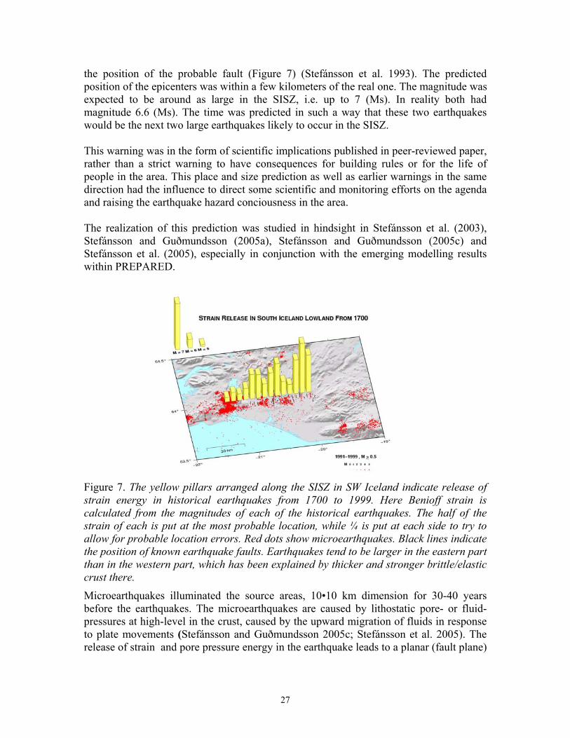
the position of the probable fault (Figure 7) (Stefánsson et al. 1993). The predicted position of the epicenters was within a few kilometers of the real one. The magnitude was expected to be around as large in the SISZ, i.e. up to 7 (Ms). In reality both had magnitude 6.6 (Ms). The time was predicted in such a way that these two earthquakes would be the next two large earthquakes likely to occur in the SISZ. This warning was in the form of scientific implications published in peer-reviewed paper, rather than a strict warning to have consequences for building rules or for the life of people in the area. This place and size prediction as well as earlier warnings in the same direction had the influence to direct some scientific and monitoring efforts on the agenda and raising the earthquake hazard conciousness in the area. The realization of this prediction was studied in hindsight in Stefánsson et al. (2003), Stefánsson and Guðmundsson (2005a), Stefánsson and Guðmundsson (2005c) and Stefánsson et al. (2005), especially in conjunction with the emerging modelling results within PREPARED.

Figure 7. The yellow pillars arranged along the SISZ in SW Iceland indicate release of strain energy in historical earthquakes from 1700 to 1999. Here Benioff strain is calculated from the magnitudes of each of the historical earthquakes. The half of the strain of each is put at the most probable location, while ¼ is put at each side to try to allow for probable location errors. Red dots show microearthquakes. Black lines indicate the position of known earthquake faults. Earthquakes tend to be larger in the eastern part than in the western part, which has been explained by thicker and stronger brittle/elastic crust there.

Microearthquakes illuminated the source areas, 10•10 km dimension for 30-40 years before the earthquakes. The microearthquakes are caused by lithostatic pore- or fluid- pressures at high-level in the crust, caused by the upward migration of fluids in response to plate movements (Stefánsson and Guðmundsson 2005c; Stefánsson et al. 2005). The release of strain and pore pressure energy in the earthquake leads to a planar (fault plane)

27

distribution of aftershocks after the earthquake, compared so the volumetric distribution before it. This is very significant for finding the place of a near future earthquake. 3.4.2 Mapping of earthquake faults Intensive mapping work in WP4.3 and WP5.2 have resulted in new knowledge about earthquake faults in the area. In WP4.3 following results have been reported: 1. All major known surface fault segments of the South Iceland seismic zone have

been field-checked and mapped by differential GPS instruments.

2. Surface faulting of the 2000 earthquakes was more extensive than previously thought. Additional faults have been mapped and a paper published in Tectonophysics (Clifton and Einarsson 2005).

3. A simplified map of all known surface faults of the SISZ has been prepared for

general use. This map is already in use on IMO’s earthquake information website as a background to the real-time earthquake locations of the South Iceland seismic zone. The map is also to be seen on a public information sign of the Icelandic Road Administration at the epicenter of the June 21, 2000 earthquake.

4. The general map base of the Icelandic Geodetic Survey in scale 1:50000 has been

incorporated into the mapping software. Detailed maps of faults can now be produced on that base for any sub-area.

A more detailed description of this work can be found in WP4.3 of the Third Periodic Report and in Clifton and Einarsson (2005). In WP5.2 intensive work has been carried out in mapping surface faults and fissures on the Reykjanes Peninsula. The fracture map shows clearly that faults and fissures are unevenly distributed across the Reykjanes Peninsula and that the stress field across the peninsula from west to east is non-uniform. It also appears that strike-slip faults are more numerous than previously recognized and that these faults are either longer or extend farther to the north than previously recognized. When earthquakes are plotted over the fault map it can be seen that earthquake swarms are often occurring at the tips of mapped surface fault traces along strike-slip faults, indicating that these faults are still active and pose a potential hazard. A number of these swarms occurred in the weeks preceding the June 4, 1998 Hengill earthquake and again in the weeks preceding the June 17, 2000 earthquake. Further study may allow us to use this information to better predict where larger earthquakes will occur. More detailed information is found in WP3 of the Third Periodic Report and in Clifton et al. (2003).

28

3.4.3 Mapping of seismogenic faults with high accuracy using relative locations algorithm Based on the observing microearthquakes the place for the 2000 earthquakes in the SISZ had signatures in the crust decades before they occurred. (Stefánsson and Guðmundsson 2005a; Stefánsson and Guðmundsson 2005c). Fluids from below the brittle crust carried lithostatic pressures to shallow depths in the crust. These fluids and the high pore pressures which they caused created during half a century conditions for the earthquake initiation at that site. It seems that the build-up of fluid pressures at the bottom of or in the brittle crust is a slow process, much slower than the time between the consecutive earthquakes in the SISZ. The earthquakes arrange along the SISZ on faults that are perpendicular to it and with distances of the order of 10 km between them. This implies that the upwelling fluids and the pore pressure build-up controls where the earthquake occurs each time on the zone, in response to the general plate motion. So a place for a next earthquake is a volume of relatively high microseismic activity, diameter of the order of 10 km. It is probably a good first approximation to claim that the fault or hypocenter will be in the center of such a volume. However, to be able to follow the premonitory process of a new earthquake and to be able to warn for it we must acquire the utmost knowlwdge about where the becoming fault will be and the form of it. We assume that the earthquakes will occur on old earthquake faults, at least as they are at depth. The high-level seismic system, the SIL-system, used in Iceland as well as experiences in multievent location methodology makes it possible to map faults with high accuracy if sufficiently many similar earthquakes occur on their fault planes. Very low seismic activity in the SISZ before the two 2000 earthquakes made it impossible to use microearthquake locations to accurately map the locked fault planes, before the earthquakes occurred. The few earthquakes that occurred did not align to or define possible fault planes. These earthquakes, deep or shallow, mostly occurred as a response to elevated pore pressures, at favourable conditions outside the fault plane in volume-shaped swarms (Stefánsson and Guðmundsson 2005c). Too few earthquakes occurred on the real fault planes, until the large 2000 earthquakes occurred. It is, however, significant to know very exactly the position of the becoming fault to be able to follow the infinitesimal motion and small microearthquakes that precede the onset of the earthquake (Stefánsson and Guðmundsson 2005a). The increased aftershock activity following the June 2000 events illuminated innumerous faults and clusters in southwestern Iceland. Many of the large historical faults in the SISZ were activated. Although many of these faults could not be mapped as a whole, since in many cases only separate patches on each fault was illuminated, these fault maps are very valuable for accurate positioning of future probable faults, i.e. with hypocenter accuracy of the order of 30-70 m.

29

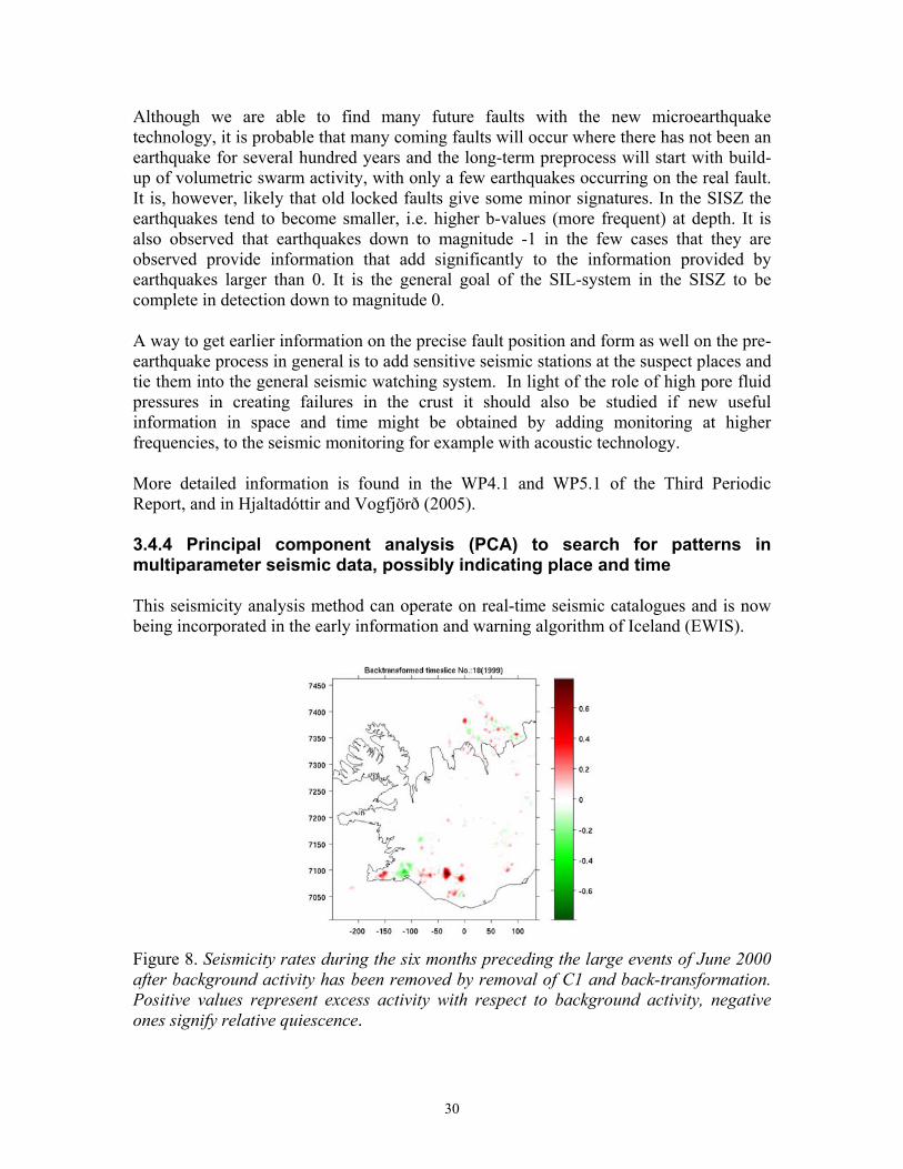
Although we are able to find many future faults with the new microearthquake technology, it is probable that many coming faults will occur where there has not been an earthquake for several hundred years and the long-term preprocess will start with build-up of volumetric swarm activity, with only a few earthquakes occurring on the real fault. It is, however, likely that old locked faults give some minor signatures. In the SISZ the earthquakes tend to become smaller, i.e. higher b-values (more frequent) at depth. It is also observed that earthquakes down to magnitude -1 in the few cases that they are observed provide information that add significantly to the information provided by earthquakes larger than 0. It is the general goal of the SIL-system in the SISZ to be complete in detection down to magnitude 0. A way to get earlier information on the precise fault position and form as well on the pre-earthquake process in general is to add sensitive seismic stations at the suspect places and tie them into the general seismic watching system. In light of the role of high pore fluid pressures in creating failures in the crust it should also be studied if new useful information in space and time might be obtained by adding monitoring at higher frequencies, to the seismic monitoring for example with acoustic technology. More detailed information is found in the WP4.1 and WP5.1 of the Third Periodic Report, and in Hjaltadóttir and Vogfjörð (2005). 3.4.4 Principal component analysis (PCA) to search for patterns in multiparameter seismic data, possibly indicating place and time This seismicity analysis method can operate on real-time seismic catalogues and is now being incorporated in the early information and warning algorithm of Iceland (EWIS).

Figure 8. Seismicity rates during the six months preceding the large events of June 2000 after background activity has been removed by removal of C1 and back-transformation. Positive values represent excess activity with respect to background activity, negative ones signify relative quiescence.

30

The method serves to separate superimposed seismicity patterns stemming from different causes, for example background seismicity, to make it easier to study earthquake premonitory patterns. Figure 8 shows seismic rates six months preceding the June 2000 earthquakes by such a search. The highest rates shown in this figure are at the Hekla volcano, at the eastern end of the SISZ, 25 km east of the initial earthquake. The volcano Hekla had an eruption 3-4 months before the earthquakes occurred. The excess activity observed at Hekla is probably related to the volcanic activity. But the eruption as well as other activity seen on the eastward prolongation of SISZ can both possibly be related to plate motion preceding the large earthquakes in the center part of the zone. The program for running PCA is ready for installation in the EWIS system at the IMO in Iceland for continuous evaluation of seismic activity. When operationally started and after some tests it will be one of the tools used to find the probable place and time of an imminent earthquake. Further information about the methodology can be found in WP2.1 of the Second Periodic Report, as well as in Goltz and Böse (2002) and Golz and Davidson (2005). 3.4.5 b-values in the SISZ to detect asperity By studies of b-values from microearthquakes in the area it was demonstrated how it can be applied to find an asperity of a future earthquake and other features describing the fault area. Studies of b-values of microearthquakes in the SISZ before the two large earthquakes could identify the asperities of the earthquakes as limited areas with low b-values, supporting the ideas that asperities with short local recurrence times control locations of major ruptures. Mapping of b-values in cross-sections of SISZ shows also anomalies of high b at the bottom of the seismogenic crust, supporting the view of high pore fluid pressures there, and correlating with the change the thickness of the brittle crust in the middle of the SISZ (Wyss and Stefánsson 2005; Figure 9).

31

Figure 9. Maps of b-values in cross-sections (color bar) along a 15 km wide EW strip in the SISZ. The two hypocenters of the large earthquakes are marked by stars. The initial earthquake is the star farther to the east. A double line delineates the approximate bottom of the dense seismic activity. The data period is 1991-2000, i.e. before the first large earthquake. 3.4.6 Strain build-up in the South Iceland seismic zone based on GPS before the 2000 earthquakes As seen in Figure 10 high strain rate is observed densely along the SISZ between 63.9ºN and 64.0ºN, coinciding with the narrow defined SISZ seen in microseismic distribution The strain build-up is interpreted as stemming from continuous 16-20 mm/year left-lateral slip at depth over a 8-11 km deep locked crust, in agreement with the expected thickness of the seismogenic layer (Árnadóttir et al. 2005a).

32

Figure 10. The strain field in the pre-seismic period 1992-2000. The northward gradient of the eastward velocity component showing left-lateral motion on EW faults, or right-lateral motion on NS faults. Another outcome of the GPS study, also including postseismic studies, is that the coseismic stress increase along the SISZ towards both ends of the zone, continues to be loaded by the post-seismic deformation (Árnadóttir et al. 2005b). 3.4.7 Estimation of the general rock stress tensor in the area Much activity has been on studying rock stress tensor of the SISZ ahead of the earthquakes, mostly by inverting fault plane solutions of microearthquakes and also by evaluation of slips from surface fracture. The average rock stress tensor of the area can most simply be expressed by maximum stress being horizontal compression striking 45ºE from N (Angelier et al. 2005; Stefánsson et al. 2005). Any variations from this are significant to detect possible stress anomalies in time and thus closeness to fracture criticality. Significant variations have been found from the avarage stresses both in space and time approaching the 2000 earthquakes but also differences between before and after the earthquakes (WP5.6 of the Third Periodic Report). These changes are discussed in Stefánsson et al. (2005). Figure 11 shows significant variations with depth between before and after the earthquakes.

33

5-10 km Az. Pl.

Before σ1 52 6

σ3 144 12

During σ1 45 18

σ3 130 13

After σ1 12 19

σ3 105 7

0-5 km Az. Pl.

Before σ1 43 4

σ3 132 8

During σ1 50 5

σ3 138 13

After σ1 23 2

σ3 113 7

Figure 11. Stress tensor inversion for the southwestern part of the Hestfjall fault. Three periods of time are considered (before, during and after the seismic crisis) and the two different depths. The observed spatial deviation of stress with depth is attributed to an effect of the pore or fluid pressures beneath five km depth or to rheological contrasts. The table below shows stress directions σ1 and horizontal compression in area around three earthquakes, the two 2000 earthquakes and an earthquake in 1988 farther west in the SISZ as studied in WP2.4 of the Third Periodic Report. J17/2000 area: 1991-1995 S1 N51°E plunge 30 SH N52°E 1996-2000 N54°E 20 N54°E 2000-2003 N58°E 20 N57°E J21/2000 area: 1991-1995 S1 N50°E plunge 5 SH N51°E 1996-2000 N43°E 20 N44°E 2000-2003 N34°E 35 N31°E Ölfus area: 1991-1995 S1 N37°8E plunge 45 SH N37°E 1996-2000 N35°E 30 N36°E 2000-2003 N28°E 30 N28°E Also in WP2.4 local variations have been studied. See discussion in WP2.4 of the Third Periodic Report and Stefánsson et al. (2005) and Lund et al. (2005). A very significant indication is that for the June 17 earthquake the deepest earthquakes below 7.5 km tend to be normal faulting in contrast to the strike-slip faulting predominant at the shallower depths. Although this local and time-dependent variation is not fully understood yet, it is probable that it involves new understanding of the earthquake preparatory process. Many

34

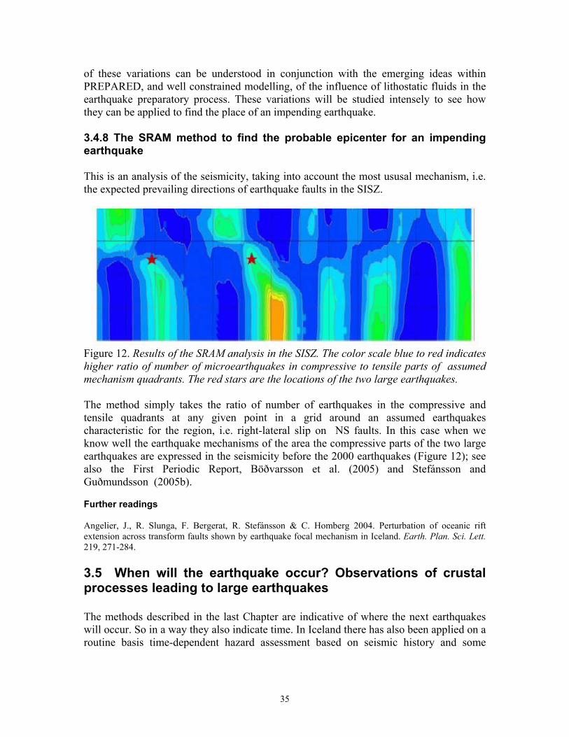
of these variations can be understood in conjunction with the emerging ideas within PREPARED, and well constrained modelling, of the influence of lithostatic fluids in the earthquake preparatory process. These variations will be studied intensely to see how they can be applied to find the place of an impending earthquake. 3.4.8 The SRAM method to find the probable epicenter for an impending earthquake This is an analysis of the seismicity, taking into account the most ususal mechanism, i.e. the expected prevailing directions of earthquake faults in the SISZ.

Figure 12. Results of the SRAM analysis in the SISZ. The color scale blue to red indicates higher ratio of number of microearthquakes in compressive to tensile parts of assumed mechanism quadrants. The red stars are the locations of the two large earthquakes. The method simply takes the ratio of number of earthquakes in the compressive and tensile quadrants at any given point in a grid around an assumed earthquakes characteristic for the region, i.e. right-lateral slip on NS faults. In this case when we know well the earthquake mechanisms of the area the compressive parts of the two large earthquakes are expressed in the seismicity before the 2000 earthquakes (Figure 12); see also the First Periodic Report, Böðvarsson et al. (2005) and Stefánsson and Guðmundsson (2005b). Further readings Angelier, J., R. Slunga, F. Bergerat, R. Stefánsson & C. Homberg 2004. Perturbation of oceanic rift extension across transform faults shown by earthquake focal mechanism in Iceland. Earth. Plan. Sci. Lett. 219, 271-284. 3.5 When will the earthquake occur? Observations of crustal processes leading to large earthquakes The methods described in the last Chapter are indicative of where the next earthquakes will occur. So in a way they also indicate time. In Iceland there has also been applied on a routine basis time-dependent hazard assessment based on seismic history and some

35

assumptions about tectonic evolution (WP5.4 in the Third Periodic Report; Halldórsson and Stefánsson 2005). In this Chapter we will more concentrate on methods leading to actions, first scientific watching actions and at last warnings that directly aim at mitigating risks for people and society. We will mainly mention some methods and results that have been tested in hindsight studying of preprocess of the June 2000 earthquakes in SISZ.

3.5.1 “Successful time predictions” in Iceland and the prospects In the following Chapters we will mainly mention some methods and results that have been tested in hindsight studying of preprocess of the June 2000 earthquakes in SISZ. Warning for a probably impending earthquake was issued 26 hours before the second earthquake occurred on 21 June, 2000. A map (Figure 13) was then sent to the Civil Defence of Iceland, indicating the most likely fault and destruction area of an earthquake that might be as large as the first earthquake (Ms=6.6) or possibly smaller. The time of it was not predicted, but the Civil Defence was advised to prepare for that it might occur any time shortly.

Figure 13. To the left is the map that was sent to the Civil Defence 26 hours before the Ms=6.6 earthquake on June 21. The boxes indicated the area of most probable destruction. Dots indicate small earthquakes in the area after the first earthquake occurred 20 km further east. The larger box was assumed most likely to become the destruction area. To the right the earthquake fault of the June 21 earthquake has been included in the map, i.e. the red line, striking right through the box of the predicted most probable hazard area. This warning was useful. It had to be made because there was a lot of observations which underbuilt it. However, there was no statistical basis for saying how probable it really was that this earthquake would occur. The basis of this warning was that from history a second earthquake should be expected in the zone, more likely to the west of the first one. Secondly the idea among the most experienced watchers about 5 km/day migration rate of earthquake activity along the SISZ (Stefánsson et al. 2003; Stefánsson and

36

Guðmundsson 2005c). What, however, pointed out really where the earthquake would strike and how large it should be expected came from the microearthquake distribution during the 3-4 days lasting between the earthquakes, illuminating a probable earthquake fault (Figure 13).

3.5.2 Seismicity rate expressing stress changes preceding the 2000 earth-quakes Figure 14 shows a cumulative number of microearthquakes, in some areas of the SISZ/RP approaching the large 2000 earthquakes.

. Figure 14. Cumulative frequency of microearthquakes above limit of completeness, approaching the 2000 earthquakes at various sites of seismic activity along the SISZ. They indicate stress increase in the epicenter of the first of the 2000 earthquakes (Ms=6.6), and near the western end of the acive part of RP, where the dynamically triggered aftershocks occurred. The areas of the study are shown to the right (Stefánsson and Guðmundsson 2005a). The gentle increase in number in the lower part of the figure, especially from the year 1996 implies stress increase (Stefánsson and Guðmundsson 2005a). The two sites shown in the lower time graph show the western and the eastern end of the active part of the SISZ/RP and show a gentle increase, as is expected when stress is building up. It appears as if much of the slip motion within the zone as a whole occurred during relatively low stresses, moved relatively easily, only building up stresses near both ends of the active part of the zone.

3.5.3 Monitoring seismicty by SAG to forecast earthquakes and eruptions The problem of using simple earthquake counting for descibing stress build-up is hampered by earthquakes releasing local stresses, and thus not expressing the general stress build-up. Several methods have been tried to cope for this, i.e. to get rid of earthquakes that depend on other earthquakes, aftershocks, etc. The method studied here

37

uses similarity in focal mechanisms to isolate dependent earthquakes, leaving solitary events to see stress changes. Figure 15 shows the result of this since 1991. The most recent brown line of the figure shows the 2000 earthquakes. It is not understood so far how this can be used in warning procedures, but studies are ongoing in trying to understand this better and to correlate it with other observations and modelling results. A more detailed information can be found in WP2.4, and in Stefánsson and Guðmundsson (2005b). A description of the SAG method is in Lund and Böðvarsson (2002). The algorithm is being introduced into the EWIS system, for monitoring and for testing and comparing with other observations of time patterns.

Figure 15. Result of Spectral Amplitude Grouping (SAG) of 8375 events in the June 17 earthquake source area. The number of solitary events (red line) and the number of groups (blue line) for an event memory of 250 events are plotted in time. Years are noted at the top and delineated by green dashed lines. The vertical, light blue lines correspond to times of volcanic eruptions in South/Central Iceland and the brown lines correspond to times of major earthquakes, above magnitude 4.5, the last line indicates the 2000 earthquakes.

3.5.4 Depth variations indicating stress variations Fluid that migrate from lithostatic depths into the crust cause near lithostatic pore pressures at shallow depths in the crust, helping to release earthquakes by reducing the normal pressure on fault planes. A corollary of this is that microearthquakes at shallow depths in the crust should indicate high local stresses. A problem of using the shallowness for stress monitor is that when the stresses overide fracture criticality they cause stress fall by the resulting earthquakes. A special case of this is when fractures get through the boundary between lithostatic to hydrostatic pressure conditions.

38

Figure 16. The depth to earthquakes with time. 30 days median value in the most active area around the epicenter of the June 17 earthquake. To plot the time history of Figure 16 we have selected the most active area around the June 17 earthquake to try to monitor the stress increase. The reason to select a limited area is that there seems to be an interplay between the various stress outlets of the area. The level in a nearby area may lose “stress” while the other is gaining. Expected long-term strain build-up in this area does not appear continuous. What we see in this figure is increasing number of fluid intrusions up in the crust, especially since 1996. With probably gradually increasing strain around the area shallow depths become more frequent, especially after a stress pulse in 1996. There are relatively more shallow earthquakes on the later half of the graph, i.e. higher stresses were indicated. It is interesting that there are more indications about stress increase during 1996, usually attributed to intrusive activity in the Vatnajökull area, above the Iceland mantle plume before a large eruption beginning of October 1996. (Crampin et al. 1999) This is in line with stress increase before the June 17 earthquake as expressed in continuous microearthquake rate increase since 1996, as seen earlier in this report.

39

Figure 17. The medians of earthquake depths after the first earthquake, but in the hypocentral area of the second earthquake, which was triggered by the first. In Figure 17 we see deepening of earthquakes with time, i.e. lowering of stress, near the occurrence of the second earthquake, just before it occurred, i.e. on June 21. This indicates that there was a stress reduction during 3 days before the earthquake. In fact the seismic rate of microearthquakes also indicates stress decay with time between the times of the two earthquakes. The explanation is in accordance with our emerging model for the nucleation of an earthquake. The second earthquake was triggered by the first. We see much stress release just after the triggering, which started the earthquake process at depth at the southern end. Slow slip which started there soon after the June 17 earthquake migrated towards north, to the hypocenter and triggered the earthquake. It migrated also towards south. Fluid pressure that constituted a part of the initial stress conditions around the fault migrated along it in response to the beginning motion, and took the role to homogenize the stress field along the fault, and thus making movement along the whole fault possible. This homogenization of the stress means also that the microearthquakes distribute along the fault instead of distributing high up in the zone. In other words to conserve energy, when spreading out laterally, the stress becomes lower and the earthquakes deeper. The depth/stress considerations have been discussed in more detail by Stefánsson and Guðmundsson (2005a).

40

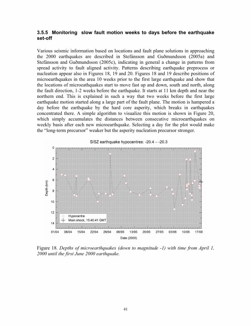
3.5.5 Monitoring slow fault motion weeks to days before the earthquake set-off Various seismic information based on locations and fault plane solutions in approaching the 2000 earthquakes are described in Stefánsson and Guðmundsson (2005a) and Stefánsson and Guðmundsson (2005c), indicating in general a change in patterns from spread activity to fault aligned activity. Patterns describing earthquake preprocess or nucleation appear also in Figures 18, 19 and 20. Figures 18 and 19 describe positions of microearthquakes in the area 10 weeks prior to the first large earthquake and show that the locations of microeathquakes start to move fast up and down, south and north, along the fault direction, 1-2 weeks before the earthquake. It starts at 11 km depth and near the northern end. This is explained in such a way that two weeks before the first large earthquake motion started along a large part of the fault plane. The motion is hampered a day before the earthquake by the hard core asperity, which breaks in earthquakes concentrated there. A simple algorithm to visualize this motion is shown in Figure 20, which simply accumulates the distances between consecutive microearthquakes on weekly basis after each new microearthquake. Selecting a day for the plot would make the “long-term precursor” weaker but the asperity nucleation precursor stronger.

Figure 18. Depths of microearthquakes (down to magnitude -1) with time from April 1, 2000 until the first June 2000 earthquake.

41

Figure 19. Epicenters of microearthquakes along a horizontal strip along the NS elongated fault plane of the first 2000 earthquake.

Figure 20. Accumulated distances between consecutive microearthquakes with time. A week is selected as a coincidence period. The figure to the left shows accumulated depths, while the figure to the right shows accumulated distance changes along the fault, i.e. latitudes. These results are not shown here to demonstrate that we have found the final algorithm to make a short-term prediction. We have simply seen a preprocess to an earthquake which starts at the bottom of the seismogenic crust. It remains to see by statistical study in what way it can be used in warning procedures. How often have similar events happened before and are there some differences which tell us if they are forerunners or not?

42

3.5.6 EQWA - a new short-term seismic warning algorithm ready for installation An alert system has been operated in the IMO center in Reykjavik since 1993. It provides alerts when predefined activity thresholds are exceeded in predefined regions, number of earthquakes, strain release in earthquakes, magnitudes and some derivatives of these. The threshold parameters of this alert system have gradually been adjusted to experience. This alert system has been significant to attract the attention of scientists, for a closer look, when the activity is unusual. Within WP3.1 a new seismic warning algorithm has been developed. The algorithm analyzes multiparameter information from microearthquakes with the aim of providing short-term warnings. The algorithm is based on the experience, that if we observe small enough earthquakes, down to magnitude 0, all big earthquakes (magnitude 4.5 and larger) since 1991 are preceded by foreshock activity (Slunga 2003), and that the breaking of a fault asperity is responsible for late foreshock activity. The EQWA algorithm provides alerts if a combination of some parameters exceed some level of probability within a small area, i.e. the area containing the asperity. It indicates the place of the pretended asperity and warning time when predefined levels are exceeded (Slunga 2005a; Slunga 2005b). The most significant parameters used are absolute stress estimations, calculated from fault plane solutions of the microearthquake, the value 1/b, which is a measure of material strength, i.e. low b-values, fault radius of the microearthquakes and activity rate. The absolute stress estimations are very significant here. They are based on very accurate fault plane solutions of microearthquakes, and on the assumption of known lithostatic fluid pressure at depth in the crust. Figure 21 shows result of EQWA for a period from 1992-2000 when the large earthquakes occurred. There are 184 warning exceedences during these 8 years, mostly shown as yellow circles. The black circles show the the exceedences during the week before the earthquakes, and they are exactly in the focal region of the first large earthquake. Most of the yellow circles are in dense clusters and near the June 21 earthquake.

43

Figure 21. A map of the SIL-area showing the EQWP for earthquakes with depth below 4 km before the June 17, 2000 earthquake. The black circles are observations within 7 days before the earthquake, only previous observations equal to or larger than the largest black circle are shown. Of the 184 exceedences most are within short-time periods, i.e. clustered activity. The cross marks the epicenter of the June 17 earthquake. In Figure 22 we only see one yellow circle for each week. The black circles are all exceedences within 7 days before the first large earthquake. So we only see three false alarm weeks during 8.5 years since 1992 until the June 17, 2000 earthquake.

44

Figure 22. The same as Figure 21 but now only the first exceedence within a 7 day period is shown. Thus each not black circle marks an alarm period of one week. There are three false alarms, one at the epicenter of June 17 earthquake and two close to the epicenter of the later June 21 earthquake. More information about this work is given in WP3.1 of the Third Periodic Report, Slunga (2003), Stefánsson and Guðmundsson (2005a) and Stefánsson and Guðmundsson (2005b). After some more statistical tests this algorithm can be introduced in the early warning system of Iceland and applied for alerts referring to small size area. The visualizing tool in the EWIS system will be used to visualize and evaluate the various components of the warning parameter and of their time evolution.

3.5.7 Stress changes monitored by SWS and stress relaxation This has been an integrated part of the two PRENLAB-projects as of the PREPARED-project. The final aim has been to stress forecast earthquakes by monitoring changes in the split time between two anisotropically splitted phases of the shear waves in local earthquakes. The method of monitoring shear-wave splitting for studying stress changes (WP2.5) is a significant complement to other methods in monitoring stress. The method is based on separating a fast and slow S-waves in the ray paths. In the SISZ the method has been applied on natural earthquakes from sources near enough and deep enough to be within the critical angle for total reflection of shear waves. It seems to be a contribution to monitoring long-term build-up of stress as well as it indicates stress relaxation

45

immediately before large earthquakes (Crampin and Chastin 2003; Crampin et al. 1999; Volti and Crampin 2003). In Figure 23 we can see how stress change was monitored by shear-wave splitting time at two seismic stations in the SISZ before the 2000 earthquakes. The rays having an incidence angle 15-45º, band 1 in the figure, is according to modelling result expected to be sensitive to stress chenges (Zatsepin and Crampin 1997). Slow stress increase is observed during several months and stress relaxations during days to weeks before the earthquake as expected from modelling (Wu et al. 2005). Analysis of anisotropy by shear-wave splitting has also demonstrated that flips in polarization of shear waves, 90º flips, occur and can be observed in critically high pore fluid pressures on fault planes. This is a significant contribution to evaluate pre-earthquake processes (Crampin et al. 2002).

a)

b)

Figure 23. Red lines are temporal increases and decreases in normalized time-delays before the Ms=6.6 June 2000 earthquakes at stations a) SAU, within a few kilometers from the epicenter of the first earthquake, and b) BJA within 50 km from the epicenter in the SISZ. Methods have been developed to forecast earthquakes, by monitoring stress increase and stress relaxation. The 2000 earthquakes have been stress forecast in hindsight on basis of the observations seen in Figure 23, and earlier observations in Iceland and some other countries. There is a wish that these methods shall be transported into the EWIS system in Iceland for testing and adjusting for being an integrated part of the earthquake watching in Iceland. This has not been done so far. The WP2.5 group has now created an Expert Analysis System (Hao et al. 2005), together with a user-friendly computer screen adjustment, leading to a Shear-Wave Analysis System (SWAS) (Gao et al. 2005), which the group believes to be a major breakthrough

46

in making analysis of shear-wave splitting more readily accessible to the general seismologist. It is hoped that these methods can be implemented into the EWIS system in Iceland within a couple of months for testing and for integrating with other methods in earthquake watching. It seems that stress increase before earthquakes and stress relaxation shortly before them can be monitored by measuring shear-wave splitting from very local earthquakes, i.e. within the critical angle incidence for S-waves. Indications for stress changes can also be seen by other methods as described earlier. A work remains to compare these methods to try to find a common denominator, i.e. an earth-realistic model that can explain the multidisciplinary observations. A part of this work is to import these measurements into the earthquake watching system in Iceland, where it is best to test them. Of course SWS can already be a significant component to the multidisciplinary earthquake watching in Iceland together with other methods applied there (Stefánsson and Guðmundsson 2005b).

3.5.8 Radon anomalies observed before the 2000 earthquakes Observations of radon in borehole wells were initiated in Iceland in 1977 (Hauksson and Goddard 1981), and continued until 1993. Several indications were found in the dataset about anomalies in radon approaching earthquakes in the SISZ (Jónsson and Einarsson 1996). In the PRENLAB-projects and the PREPARED-project (WP3.2) much has been done in recompiling old data as well as developing tools for automatic evaluations of radon content. A new program of radon sampling from geothermal wells in the South Iceland seismic zone was initiated in 1999, a year before the large earthquakes of June 2000 occurred. Evaluation of the results of these observations have been carried out inside and outside the PREPARED-project. The earthquakes which occurred in the middle of the sampling network were preceded by clear anomalies at six out of seven stations (WP3.2 of the Third Periodic Report; Einarsson et al. 2005a; Theodórsson and Guðjónsson 2003; Stefánsson and Guðmundsson 2005b). The most significant finding of studying the radon anomalies before the 2000 earthquakes is the high correlation between the radon time series over the entire area in the period 1999-2001. Stations that are tens of kilometers apart show very similar fluctuations in the concentration of radon. Considering the short half-life of radon these fluctuations most likely have common origin, and that is probably related to the large tectonic events in and near the SISZ from the eruption of Hekla volcano which lasted from February 26 to the large earthquakes of June 2000. These observations as well as the post-earthquake radon observations will be a very significant contribution to understanding the mechanism of the premonitory process of the earthquakes. The radon monitoring and studies imply as the seismic studies that there is an observable premonitory earthquake process that provides a basis for warning efforts, although we do

47

not have so far a causative model to link these observations together and describe the time evolution of this process. The findings in this project have brought forward technological development that will make the radon more feasible in watching crustal strain changes (Theodórsson and Guðjónsson 2003). Continuous radon observations are now ready to be introduced in the EWIS system. Future work is needed to be better able to fully understand and to create a physical model for explaining these observations.

3.5.9 Hydrological pulse observed 24 hours before the first earthquake In a geothermal borehole at Flúðir 10 km to the north of and in line with the NS-striking fault plane (Figure 24), short-term water level drop of not less than 5 m, was alarmed 24 hours before the earthquake. Unfortunately this signal is not seen in the preserved recorded trace averaging water level on 15 minutes intervals. During a 5 years of continuous operation this was the first such an alarm (Björnsson et al. 2001). Most probably the alarm was a short-lived pulse of reduced waterheight related to the preparatory phase of the earthquake. Although the recording of this was not preserved it has to be considered significant. It is interesting that the alarm was at the time of the clustering of the pre-earthquake seismicity at the asperity. As described in Chapter 3.5.5 the nucleation process started by slow slip at depth, hampered during the last 24 hours before the earthquake or so by the strong asperity before it broke. Such an abrupt stopping may have led to abrupt minor strain changes in the surroundings. The strain changes may have caused a hydrological signal in the borehole which is drilled in a crack in area with deep roots of water supply hit by the strain change. Such a signal can be very short-lived, diffusing into the surrounding area and thus not seen even in a 15 minute record (Stefánsson and Guðmundsson 2005b). This signal should be modelled more profoundly to consider how such a signal can be used for short-term warnings or alerts. It is already on the plan to link water depths in several boreholes to the routine warning procedures at IMO.

48

Figure 24. An area near the June 17 earthquake. The epicenter is shown by a green star and the rupture is indicated with a red NS striking line. The NS-striking black lines indicate some old earthquake faults. Red dots show microearthquakes (36 in number, ML=-1 to 1), during a period of 17 days before the earthquake. Hydrological changes were observed at the village Flúðir as reported in text. Hydrological postseismic changes have been studied in WP5.5, which has among others studied the effect of fault slip on fluid transport, especially geothermal water at shallow depths (i.e. above the lithostatic/hydrostatic boundary at about 3-4 km depth) (Guðmundsson and Geyer 2005). InSAR measurements revealed deformation due to ground water movements during the two months following the earthquakes (Jónsson et al. 2003).

3.5.10 Earthquake triggering by another observable event To understand earthquake triggering is of course significant for predicting some earthquakes. As has been discussed and modelled the second large earthquake in June 2000 was triggered by the first and our understanding of the seismic history and pre-earthquake seismic patterns made it possible to warn for it as was described earlier. Among the most spectacular observations after the 2000 earthquakes was the triggering of a number of medium-large earthquakes up to distances of 100 km along the SISZ. This was modelled as dynamic triggering assuming rate- and state-dependent fault rheology which could explain a wide temporal spectrum of triggering effects. The origin of the triggered events correlated with the arrival of seismic waves. A condition for the triggering was high pore pressure values in the fault regions before the triggered events occurred (Antonioli et al. 2005; Stefánsson et al. 2005). 3 1/2 month before the 2000 earthquakes there was an eruption in the volcano Hekla, which is at the eastern end of the SISZ. The Hekla volcano has erupted approximately every tenth year since 1970, which is considered unusually frequent. It has often been

49

suggested that it may have to do with the strain conditions in the SISZ. This connection as well as the connection between the 2000 SISZ earthquakes and tectonic activity at Hengill volcano at the other end of the SISZ has been studied by Guðmundsson (2005) and Guðmundsson and Brenner (2005). There are indications based on some examples of seismic history as well as on recent observations that large seismic events tend to migrate approximately with a velocity of 5 km/day. This was taken into account in predicting the June 21, 2000 earthquake. The actual velocity between the two June 2000 epicenters was 4.9 km/day. (Stefánsson et al. 2003). This has not been studied by modelling and the mechanism controlling such results is not yet understood. In Appendix 1 of the Third Periodic Report, Kurt Feigl reports some international results to compare with this. A work awaits to study this in detail and to model it. Further readings Árnadóttir, Þ., H. Geirsson & P. Einarsson 2004. Coseismic stress changes and crustal deformation on the Reykjanes Peninsula due to triggered earthquakes on 17 June 2000. J. Geophys. Res. 109, B09307. Einarsson, P., P. Theodórsson & G.I. Guðjónsson 2005. Radon anomalies prior to the earthquake sequence in June 2000 in the South Iceland Seismic Zone. Geophys. Res. Lett. Manuscript under revision. Soosalu, H. & P. Einarsson 1997. Seismicity around the Hekla and Torfajökull voncanoes, Iceland, during a volcanically quiet period, 1991-1995. Bull. Volcanol. 59, 36-48. Soosalu, H., P. Einarsson & B.S. Þorbjarnardóttir 2005. Seismic activity associated with the 2000 eruption of Hekla, Iceland. Bull. Volcanol. 1432-0819 (online). Sturkell, E., P. Einarsson, F. Sigmundsson, H. Geirsson, R. Pedersen, E. van Dalfsen, A. Linde, S. Sacks & R. Stefánsson 2005. Volcano geodesy and magma dynamics in Iceland. J. Volc. Geotherm. Res. In press. 3.6 Improving hazard assessments and time-dependent assessments of probable earthquake effects In Chapter 2.1 we defined our approach to earthquake warnings or prediction which in our definition is equivalent in general to the the role of earth sciences in mitigating seismic risk. We try to provide (time-independent) probabilistic hazard assessment, time-dependent hazard assessment, short-term warnings and early warnings or ”nowcasting”. Nowcasting means to provide basic information about an earthquake that has occurred, for mitigating its risk effects. However, such a nowcasting is included in all pre-warning procedures. That is to say at all stages in our pre-warnings we provide similar kind of information as in the nowcasting after the earthquake has occurred. The difference is that nowcasting is based on the observations of the earthquake after it has occurred while the pre-earthquake information is based on the predictions we make about the probable effects of the potential earthquake. Anyhow the basic information in our warnings is to assess as well as possible and as early as possible the exact location, and surface effects of the large earthquake, before and after it occurs.

50

In the following a few basic results are described that will help in future hazard assessments, time-independent and time-dependent.

3.6.1 Some results of PREPARED that will help in enhancing the hazard assessments The probabilistic hazard assessment is usually mainly based on applying statistical methods to imply what a probability is for large earthquakes in a region. Also often based on assuming the largest probable earthquake as estimated from tectonic understanding. So it has been done in the hazard assessment in Iceland. In the following some results are mentioned that have been described earlier in this report and how these help to enhance hazard assessment. Hazard assessment in Iceland is mainly based on list of historical earthquakes since year 1700, estimated locations and magnitudes. The observations of the year 2000 earthquakes imply no significant revision of the magnitudes and only minor revision of the earthquake locations (Halldórsson and Stefánsson 2005).

3.6.1.1 The significance of the new modelling The basic modelling reported here implies that fluids from depth can penetrate from the brittle/ductile boundary up through the crust. This tends to build up pore-fluid pressures in the crust especially around fissures and faults, where they are also released. These fluids carry lithostatic pressure up into the earthquake damage zone and modify the conditions for earthquake release there in response to plate motion strain. They help to release microearthquakes which are used to map faults at depth, which are used for studying the pre-earthquake conditions and changes, and which are used to detect and follow the nucleation phase of a possibly large earthquake (Stefánsson et al. 2005c). This model explains several other observations which can be applied to study the physical processes ahead of earthquakes (Zencher et al. 2005). 3.6.1.2 To identify the dangerous fault Much work has been carried out to locate faults of earlier earthquakes in the SISZ by geological mapping (Clifton and Einarsson 2005; WP4.3 of the Third Periodic Report). Not all faults of old earthquakes can be found by geological mapping. Also it is difficult in most cases to find the extension and form of the fault at depth, which is significant for assessing the potential fault size and accelerations or intensity at various places. The 2000 earthquakes “illuminated” old earthquake faults in the SISZ, by reactivating them. Microearthquake recording of this and older observations made it possible to map old faults with place and size at depth in the crust (Hjaltadóttir and Vogfjörð 2005).

51

The identified large earthquake faults in the SISZ create a dense fabric, mostly 10-20 km long of parallel NS faults of the order of 6 km apart from each other. This is the case with earthquakes since 1700. The hegemony of processes at depth in faulting the crust in earthquakes implies that new earthquakes do not necessary occur at these faults. There are indications that the fault fabric may be even denser (Wyss and Stefánsson 2005). It has been found in this study that processes that start nucleating earthquakes may start years or decades ahead of the earthquakes. Methods have been outlined which make it possible to locate build-up of future faults and future asperities, meaning to help to answer the question where will the next large earthquakes occur, and gradually what will be its size. 3.6.1.3 Slip inversion models Evaluations of accelerometer observations available during the earthquakes as well as GPS and microearthquake observations have been applied to constrain a variable slip mode of the earthquakes. This slip model has then been used to calculate expected accelerations on a dense scale. These results can be applied to go from a predicted fault model of an earthquake to predict its size or severity at any point, knowing the crustal structure including estimations of shallow side effects. A special case of this is to use new information at any step in approaching the large earthquake to predict its severity on basis of the new and emerging understanding of the probable fault process. The closer we come to the earthquake the better we should understand the expected fault process and thus to predict better its expected severity at any point.

3.6.1.4 From “classical” hazard assessment to dynamic hazard assessments The hazard assessment goes from the classical time-independent hazard assessment to time-dependent hazard assessment that must be renewed at any time of new information about the potential earthquake. All basic information about probable earthquake size, earthquake faults, crustal structure and surface conditions, as well as an emerging model for the probable earthquake, we keep in an easily acessible database, for making new models on basis of new observations. A significant part of this dynamic hazard assessment is thus our technics in detecting and observing pre-earthquake changes. For this we have developed alert algorithms and methods for visualization and fast evaluations of an crustal processes. I described earlier the alert algorithms and some methods to watch crustal processes related to earthquakes. To handle these evaluations, to deseminate these and to create a common table for scientists and civil defence to cooperate, the IMO has created the Early Warning and Information System (EWIS), as well as an activating and continously operating alert system.

3.6.1.5 Attenuation of strong ground motion and site effects Attenuation of horizontal peak ground acceleration of the 2000 earthquakes were applied to find a curve describing attenuation in the near as in the far field (Ólafsson and

52

Sigbjörnsson 2004). On basis of acceleration records site effects have been calculated by the Nakamura H/V method (Ólafsson and Sigbjörnsson 2005). Further readings Angelier, J., F. Bergerat, M. Bellou & C. Homberg 2004. Co-seimsic strike-slip displacement determined from push-up structures: the Selsund Fault case, South Iceland. Journ. Struct. Geol. 26, 709-724. Bergerat, F. & J. Angelier 2003. Mechanisms of the June 2000 earthquakes, southern Iceland: inferences from surface traces of the Árnes and Hestfjall faults. Journ. Struct. Geol. 25, 1507-1523. Halldórsson, P. & B.I. Sveinsson 2003. Dvínun hröðunar á Íslandi (Attenuation of acceleration in Iceland). Icelandic Meteorological Office – Report 03025. Richwalski, S.M. & F. Roth 2005. Inelastic shear and Coulomb stress changes in the South Iceland seismic zone due to strong earthquakes since 1706. Tectonophysics. Submitted. Sigbjörnsson, R. & S. Ólafsson 2004. On the South Iceland earthquakes in June 2000: strong-motion effects and damage. Bolletino de geofisica – teorica ed applicata. An International Journal of Earth Sciences 45(1-2), 131-152. 3.7 The Early Warning and Information System of Iceland (EWIS) The Early Warning and Information System of Iceland (EWIS) for geological hazards, was initiated after the recent successes in providing warnings ahead of earthquake and volcanic hazards. This system is already in use and has recently shown its usefulness in warnings before a glacial flood and volcanic eruption. (Roberts et al. 2005a; Vogfjörð et al. 2005). Although in practical use, it is also in development by IMO and by some cooperators. This system comprises a database, a GIS server, and a dedicated website. The data handling procedures and GIS techniques within this system is already in use for fast evaluations of observations. Alongside our 15-year digital record of earthquakes in Iceland, we are building a supplementary database for the centralized storage and visualization of GIS resources such as hazard maps, aerial photographs, satellite images, and published geological and geophysical data. Additionally, IMO is a participant in FORESIGHT – an ongoing EC project with the goal of understanding the mechanically coupled, interrelated processes leading to hazardous activity associated with earthquakes, volcanic eruptions, landslides, and tsunamis. This project makes full use of temporal GIS techniques to create web-based hazard maps for use in risk mitigation work, during periods of hazards or ahead of them on basis of observed premonitory changes. The EWIS system is a tool for real-time research of scientists in the watching center (IMO) or outside the watching center among cooperators, even in other countries. During period of observations that may be preceding earthquakes or other hazards and during hazard situation it is significant to attract all scientists that can provide help in the real-time research to a common worktable.

53

It is a tool for dissemination of information to governmental agencies and the public. Of a special significance is interactive communication with the Civil Defence of Iceland. most warnings, especially ahead of earthquakes are issued through that department or in conjunction with it. An alert system operates as an integrated part of the EWIS and the watching activities at IMO. Several algorithms can now be introduced into this alert system based on results of the PREPARED-project in addition to the alerts algorithms that are operated there for the time being. The earthquake watching involves alerts or short-term warnings, median- and long-term assessments as well as scientific evaluations or real-time research. Further readings Roberts, M.J., R. Stefánsson, P. Halldórsson & E.Þ. Hvannberg 2005b. Internet-based platform for real-time geoscience during tectonic crisis in Iceland. In preparation. 3.8 Advances in providing early information and warnings about earth-quakes In Chapter 2.1 we have described our approach to earthquake warnings or “prediction”. It is a gradual approach aiming at mitigating risks that stem from earthquakes, by foreseeing or assessing the hazard before it occurs or during the hazard period. This approach involves actions to be taken at various stages of the probability of a potential hazard in various places. These actions involve everything from enhancing significant monitoring to scientific evaluations and advices to civil defence and rescue groups. One of the main problems in earthquake predictions is that large earthquakes are not repeated in the same place under same conditions within our times of good observations. Therefore methods that are based on repetance of similar events have less chance in predicting than many other events that are often repeated. Therefore a physical approach is necessary, i.e. understanding the physical process leading to earthquakes. To understand these processes we must have multidisciplinary approach, need all the multidisciplinary observations that can be made available and the achieveable scientific level. For the same reason we must try to catch up the earthquake processes while it is in a preparatory stage. Our hope in earthquake prediction is that the processes describing the conditions in the earthquake fault area start before the earthquake. By “real-time research” and enhanced monitoring we try to describe the future development in the fault area, from the long-term assessment, or finding the suspicious fault to the possibility of providing short-term warning. This approach, the PREPARED approach, which involves in general better understanding of the physical properties of the area, will also help in gradually providing a better hazard assessment, and thus mitigate risks even if time warnings are not successful.

54

3.8.1 The PREPARED-project results in manyfold progress towards mitigating risks in this way A basic finding is an innovative and earth-realistic model which predicts that high pore pressure values can efficiently migrate from below the brittle-ductile transition to shallower depths. This model is based on earth-realistic parameters for the area and supported by various observations in the SISZ. This has often been suggested before, but within the PREPARED-project this hypothesis has been established as a working hypothesis that has been applied within many groups of the project. Methods have been developed and applied to find active faults and earthquake asperities. It has been found that all earthquakes in Iceland larger than 4.5 since the creation of the SIL microearthquake system have bee preceded by microearthquakes. Several methods for monitoring pre-earthquake processes have been described, both involving seismic measurements, radon measurements and change of water level in boreholes. In some of these it can be shown that they monitor slow fault motion that starts at depth before the earthquake, in others they show the fracturing of the asperity or stress-related fluid flow or stress relaxation. An early information and warning system (EWIS) has been developed by the coordinator alongside with the PREPARED which makes it possible to visualize and compare such processes.

3.8.2 Short-term alerts Some of the findings described in this report have been integrated in the EQWA warning algorithm that will be introduced in the warning practices at IMO shortly for testing and for regular operation. Work is ongoing and in preparation for testing and to find significance for alerts in several of the methods describing premonitory processes. It is hoped that it will be possible to implement the SWS (shear-wave splitting method) for stress forecasting earthquakes into the EWIS system of IMO for testing and evaluating within a few months. 3.9 Future research towards a further progress in earthquake warnings Even if significant results have been achieved in the PREPARED-project it is necessary to have in mind that future research is needed for more progress. Much work is needed to study the level of significance of the results for warnings. It is significant to see and be able to follow crustal processes towards earthquakes. However, much work remains to analyze these processes better to find out how significant they can be for warnings, to try

55

to establish better their statistical significance. It also remains to study how these results can be applied in other conditions at other places in the world. Even if earthquakes have many similarities wherever they occur, crustal conditions are different in different parts of the world. Iceland has a relatively thin elastic/brittle crust compared to more continental areas and it has also relatively high thermal gradient. It was shown in the project that high pore fluid pressures are prevailing below the seismogenic crust, at approximately 10 km depth. We cannot be sure that high pore fluid pressures prevail below the seismogenic crust everywhere and it is usually thicker than in Iceland. The very small earthquakes which are so significant for our progress may not exist in the same amount at other places. But this must be studied by monitoring with networks that are at least as sensitive as the Icelandic network. Among results in the project is that earthquakes below 0 even down to -1 magnitude carry information which is significant and comparable to the earthquakes above 0 or 1 in magnitude. In the original design of the SIL-system the goal was to get down to magnitude zero. Many scientists around the world at that time claimed this was far too low to be practical. It has, however, been shown in this project that earthquakes down to magnitude zero are significant. These very small earthquakes are probably abundant and it would increase our significant data more than 10 times to get down to -1 completeness in magnitudes. In this case the number matters. Therefore we should monitor with even denser station network than we have now at suspicious faults. This also awakes the question if we should go down to higher frequencies and study endogen acoustic noise at suspicious places too. In many cases in this work more modelling would be needed to explain all results. An example is the hydrological signal that made an alert 24 hours before the first of the earthquakes. In several other cases theoretical work or earth-realistic modelling has not quite followed up with the observations and intuition.

56

4 Conclusions including socio-economic relevance, strategic aspects and policy implications The human, social and economic impact of a destructive earthquake is enormous. Well established prognosis of what can be expected is a basis for decision on how and where man-made structures are built. It may lead to strengthening or removal of existing vulnerable buildings. It is a basis for various technical and social precautions and preparedness that can mitigate the impact of earthquake hazards in various ways. Many of the results of PREPARED can be applied in time-independent or time-dependent efforts to mitigate risks caused by earthquake hazard. But even if houses are well built, and especially if the are not well built to resist earthquakes, a warning ahead of an impending potentially destructive earthquake is indispensable. A significant progress is reported towards warnings for earthquake before it occurs and in predicting its effects. The PREPARED-project results are the latest results from earthquake prediction research projects that have been ongoing since 1988, in international, especially European (EC) cooperation as was described at the beginning of this report. The South Iceland seismic zone (SISZ) was nominated a European test area for earthquake prediction reseach in the early 1980’s by the Council of Europe. The concentration of Icelandic and gradually more European scientists on earthquake prediction research in the SISZ was based on a long-term earthquake prediction of large earthquakes to be expected in near future at defined sites the within the zone. This prediction was verified in the two magnitude 6.6 (Ms) earthquakes at the predicted sites in June 2000. The research work ahead of the earthquakes was significant for understanding better their effects, and it made possible to prepare a useful 26 hours warning about the size and the place of the second of the two earthquakes. But what was also significant was that the concentration of research and monitoring efforts in this area led to increased high-level monitoring in the area. Therefore much information was collected on premonitory activity before the earthquakes. This was the basis for the PREPARED-project, which now is coming to an end. But the progress of the earthquake prediction research projects in Iceland has led to new parallel projects, which are based on the SIL monitoring system and the SIL-project in 1988-1995 and other significant results. Among these projects are: The EC SMSITES-project (2000-2003), the EC RETINA-project (2002-2005), the Icelandic EWIS-project (2003-2005), all centered in Iceland, and the EC FORESIGHT-project (2004-2006) to a significant aspect based on results of multinational cooperative work in Iceland. As was said before the position of earthquake prediction in general lowered near the start of the Icelandic prediction story, before 1990. Critical views claiming that earthquake

57

prediction would probably never succeed were based on some earlier misfortunes in earthquake prediction. They influenced the research efforts in the SISZ test area in such a way to put more efforts to the physical and multidisciplinary approach rather than to the pattern search in seismic catalogues only, as had been characterizing earlier earthquake prediction efforts. The progress in the Icelandic earthquake prediction research has been descibed at conferences and by other means among scientists. This is probably one of the reasons for that earthquake prediction research has now again a higher status than for a while. It is significant that the progress of the PREPARED will be followed up by intensive work in testing and qualifying warning algorithms and procedures for monitoring processes leading to large earthquakes. Because of the lack of earthquake prediction research in other parts of the world and because of the good progress of the PREPARED-project and other earthquake prediction research projects supported by the EC, the EC has special duties toward those who live in danger for earthquake hazards to support such research work. In the PREPARED-project it has been shown that progress towards earthquake prediction is possible. We have already demonstrated significant progress which must be followed up. This will create optimism about the possibilities of scientific work and increase the quality of life. The faith in science for mitigating earthquake risk is already of enormous socio-economic significance and for the quality of life in Iceland. The experiences gained in PREPARED in Iceland can be applied in other parts of the world for encouraging work in this field and will create well based hopes that it is possible to obtain good results in earthquake prediction.

58

5 Dissemination and exploitation of the result The dissemination of results will be carried out by the individual participants through scientific journals and in popular reports and possibly books. In Iceland the results will be tested and qualified for watching purposes in the Early Warning and Information System (EWIS) and in an operating alert system. They will also be a basis for hazard assessment and risk analysis. Many of the participants will also serve as advisers in earthquake-prone areas where there is a wish for research and build-up of earthquake watching mechanism and research.

59

References Angelier, J., F. Bergerat & R. Stefánsson 2005. Seismotectonics of the newly formed transform zone near a hot spot: earthquake mechanism and regional stress in the South Iceland Seismic Zone. J. Geophys. Res. Submitted. Antonioli, A., M.E. Belardinelli, A. Bizzarri & K.S. Vogfjörð 2005. Evidences of dynamic triggering during the seismic sequence of year 2000 in South Iceland. J. Geophys. Res. Accepted. Árnadóttir, Þ., S. Jónsson, R. Pedersen & G.B. Gudmundsson 2003. Coulomb stress changes in the South Iceland Seismic Zone due to two large earthquakes in June 2000. Geophys. Res. Lett. 30(5). Árnadóttir, Þ., W. Jiang, K.L. Feigl, H. Geirsson & E. Sturkell 2005a. Kinematic models of plate boundary deformation in southwest Iceland derived from GPS observations. J. Geophys. Res. Submitted. Árnadóttir, Þ., S. Jónsson, F. Pollitz, W. Jiang & K.L. Feigl 2005b. Post-seismic deformation following the June 2000 earthquake sequence in the South Iceland seismic zone. J. Geophys. Res. Submitted. Björnsson, G., Ó.G. Flóvenz, K. Sæmundsson & E.M. Einarsson 2001. Pressure changes in Icelandic geothermal reservoirs associated with two earthquakes in June 2000. In: Proceedings of the Twenty-Sixth Workshop on Geothermal Reservoir Engineering, Stanford University, Stanford, California. Böðvarsson, R., B. Lund & A. Tryggvason 2005. Seismicity ratio with applied mechanism. In: Abstracts from the EGU General Assembly, Vienna, Austria, April 24-29, 2005. Clifton, A.E., C. Pagli, J.F. Jónsdóttir, K. Eyþórsdóttir & K. Vogfjörð 2003. Surface effects of triggered fault slip on Reykjanes Peninsula, SW Iceland. Tectonophysics 369, 145-154. Clifton, A.E. & P. Einarsson 2005. Styles of surface rupture accompanying the June 17 and 21, 2000, earthquakes in the South Iceland Seismic Zone. Tectonophysics 396, 141-159. Crampin, S., T. Volti & R. Stefánsson 1999. A successfully stress-forecast earthquake. Geophys. J. Int. 138, F1-F5. Crampin, S. T. Volti, S. Chastin, Á. Guðmundsson & R. Stefánsson. 2002. Indications of high pore-fluid pressures in a seismically active fault zone. Geophys. J. Int. 151, F1-F5.

61

62

Crampin, S. & S. Chastin 2003. A review of shear-wave splitting in the crack-critical crust. Geophys. J. Int. 155, 221-240. Einarsson, P., S. Jónsson, S. Björnsson & Á.R. Hjartardóttir 2005. Radon anomalies and earthquakes in the South Iceland Seismic Zone 1977-1993. Geophys. Res. Lett. Submitted. Gao, Y., P. Hao & S. Crampin 2005. SWAS: a Shear-Wave Analysis System for semi-automatic measurement of shear-wave splitting above small earthquakes. Geophys. J. Int. Submitted. Goltz, C. & M. Böse 2002. Configurational entropy of critical earthquake populations. Geophys. Res. Lett. 29(20), 51, 1-4. Goltz, C. & J. Davidsen 2005. Measuring the complexity of evolving seismicity. Earth. Plan. Sci. Lett. Submitted. Guðmundsson, Á. 2005. Mechanical interaction between volcanic and seismic zones in Iceland. Tectonophysics. Submitted. Guðmundsson, Á. & S.L. Brenner 2005. How local stress fields prevent volcanic eruptions. J. Volc. Geotherm. Res. Submitted. Guðmundsson, Á. & A. Geyer 2005. Damage-zone growth, local stresses, and fault displacement. Geophys. Res. Lett. Submitted. Halldórsson, P. & R. Stefánsson 2005. Reevaluation of historical earthquakes. Icelandic Meteorological Office – Report. In press. Hao, P., Y. Gao & S. Crampin 2005. An Expert System for measuring shear-wave splitting above small earthquakes. Pure. Appl. Geophys. Submitted. Hauksson, E. & J.G. Goddard 1981. Radon earthquake precursor studies in Iceland. J. Geophys. Res. 86, 7037-7054. Hjaltadóttir, S. & K.S. Vogfjörð, 2005. Subsurface fault mapping in Southwest Iceland by relative location of aftershocks of the June 2000 earthquakes. Icelandic Meteorological Office – Research Report 21, 18 pp. Hjaltadóttir, S., K.S. Vogfjörð, Þ. Árnadóttir, P. Einarsson & P. Suhadolc 2005. A model of the release of the two 2000 earthquakes based on all available observations. Icelandic Meteorological Office - Report 05020.

63

Jónsson, S. & P. Einarsson 1996. Radon anomalies and earthquakes in the South Iceland Seismic Zone 1977-1993. In: (B. Þorkelsson (editor), Seismology in Europe. Papers presented at the XXV ESC General Assembly, Reykjavík, Iceland, September 9-14, 1996, 247-252.

Jónsson, S., P. Segall, R. Pedersen & G. Björnsson 2003. Post-earthquake ground movements correlated to pore-pressure gradients. Nature 424, 179-183. Lund, B. & R. Böðvarsson 2002. Correlation of microearthquake body-wave spectral amplitudes. Bull. Seism. Soc. Am. 92, 2410-2433. Lund, B., M. Arvidsson, R. Böðvarsson & R. Slunga 2005. Crustal stress anomaly before the M=6.5 17 June 2000 earthquake in South Iceland. Geophys. Res. Lett. Submitted. Ólafsson, S. & Sigbjörnsson 2004. Attenuation of strong ground motion in shallow earthquakes. In: Proceedings of the 13th World Conference on Earthquake Engineering, Vancouver, British Columbia, Canada, 2004.

Ólafsson, S. & R. Sigbjörnsson 2005. Site effects in South-Iceland based on strong ground acceleration. Report of the Engineering Research Institute, University of Iceland. Pedersen, R., S. Jónsson, Þ. Árnadóttir, F. Sigmundsson & K.L. Feigl 2003. Fault slip distribution of two Mw=6.5 earthquakes in South Iceland estimated from joint inversion of InSAR and GPS measurements. Earth Plan. Sci. Lett. 213, 487-502. Roberts, M.J., R. Stefánsson, S.S. Jakobsdóttir, G.B. Guðmundsson, K.S. Vogfjörð & P. Halldórsson 2005a. Iceland´s Early warning and informations system for geologic hazards. In: Proceedings of the EGU General Assembly, Vienna, Austria, April 24-29, 2005. Roth, F. 2004. Stress changes modelled for the sequence of strong earthquakes in the South Iceland seismic zone since 1706, Pageoph. 161(7), 1305-1327. Slunga 2003. Microearthquake analysis at local seismic networks in Iceland and Sweden and earthquake precursors. In: Lecture Notes in Earth Sciences. Methods and Applications of Signal Processing in Seismic Network Operations. Springer Verlag, Germany. Slunga, R. 2005. Complete stress tensor estimates from single event fault plane solutions. In preparation. Slunga, R. 2005. A short-term earthquake warning algorithm based on microearthquake analysis. In preparation.

64

Stefánsson, R., R. Böðvarsson, R. Slunga, P. Einarsson, S.S. Jakobsdóttir, H. Bungum, S. Gregersen, J. Havskov, J. Hjelme & H. Korhonen 1993. Earthquake prediction research in the South Iceland seismic zone and the SIL project. Bull. Seism. Soc. Am. 83(3), 696-716. Stefánsson, R., G.B. Guðmundsson & P. Halldórsson 2003. The South Iceland earthquakes 2000 - a challenge for earthquake prediction research. Icelandic Meteorological Office – Report 03017. Stefánsson, R. & G.B. Guðmundsson 2005a. Long-term and short-term earthquake warnings based on seismic information in the SISZ. Icelandic Meteorological Office –Report. In press. Stefánsson, R. & G.B. Guðmundsson 2005b. Ahead of the earthquake: Assessment of where, how and when. Icelandic Meteorological Office – Report. In press. Stefánsson, R. & G.B. Guðmundsson 2005c. About the state-of-the-art in providing earthquake warnings in Iceland. Icelandic Meteorological Office – Report 05003. Stefánsson, R., M. Bonafede, F. Roth, P. Einarsson, Þ. Árnadóttir & G.B. Guðmundsson 2005. Modelling and parameterizing the SW Iceland earthquake release and deformation process. Icelandic Meteorological Office – Report. In press. Suhadolc, P. & D. Sandron 2005. Fault slip distribution of the two June 2000 Mw=6.5 earthquake in South Iceland estimated by strong motion inversion. In: PREPARED Second Periodic Report. Icelandic Meteorological Office -Report 05007. Theodórsson, P. & G.I. Guðjónsson 2003. A simple and sensitive liquid scintillation counting system for continuous monitoring of radon in water. Advances in Liquid Scintillation Spectrometry, 249-253. Vogfjörð, K.S., S.S. Jakobsdóttir, G.B. Guðmundsson, M.J. Roberts, K. Ágústsson, Þ. Arason, H. Geirsson, S. Karlsdóttir, S. Hjaltadóttir, U. Ólafsdóttir, B.S. Þorbjarnardóttir, Þ. Skaftadóttir, E. Sturkell, E.B. Jónasdóttir, G. Hafsteinsson, R. Stefánsson & Þ.V. Jónsson 2005. Forecast and multidisciplinary monitoring of a subglacial eruption in Iceland. EOS, Transactions, American Geophysical Union 86(26), 245, 248. Volti, T. & S. Crampin 2003. A four year study of shear-wave splitting in Iceland: 2. Temporal changes before earthquakes and volcanic eruptions. In: D.A. Nieuwland (editor), New Insights into Structural Interpretation and Modelling. Geol. Soc. Lond. Spec. Publ. 212,135-149. Wyss, M. & R. Stefánsson 2005. Nucleation points of recent main shocks in southern Iceland mapped by b-values. Bull. Seism. Soc. Am. Accepted.

65

Wu, J., Y. Gao, S. Crampin, T. Volti & Y.T. Chen 2005. Smaller source earthquakes and improved measuring techniques allow the largest earthquakes in Iceland to be stress-forecast (with hindsight). Geophys. J. Int., Fast Track. Submitted. Zatsepin, S.V. & S. Crampin 1997. Modelling the compliance of crustal rock: I - response of shear-wave splitting to differential stress. Geophys. J. Int., 129, 477-494. Zencher, F., M. Bonafede & R. Stefánsson 2005. Near-lithostatic pore pressure at seismogenic depths: a thermo-poro-elastic model. Geophys. J. Int. Submitted.

Documents

PREPARED - final report