Prepared by, Assistant Professor/Department of CS, · Top Big Data Technologies 1. Apache Hadoop • Apache Hadoop is a java based free software framework that can effectively store

Prepared by,

Ms. P.DEEPIKA M.E.,

Assistant Professor/Department of CS,

PARVATHY’S ARTS & SCIENCE COLLEGE.

UNIT I

Prepared by P.Deepika, Assistant Professor,PASC

2

What is a Data?

• Data is any set of characters that has been gathered and

translated for some purpose, usually analysis.

• It can be any character, including text and numbers, pictures,

sound, or video.


3

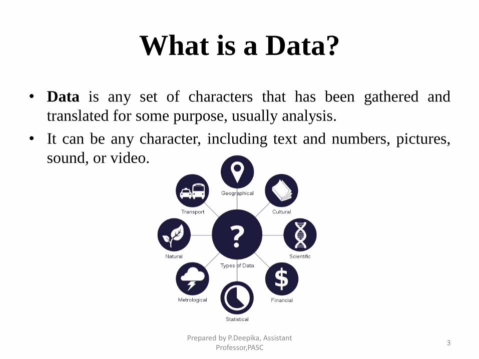
What is Digital Data?

• Digital data are discrete, discontinuous representations of

information or work.

• Digital data is a binary language.


4

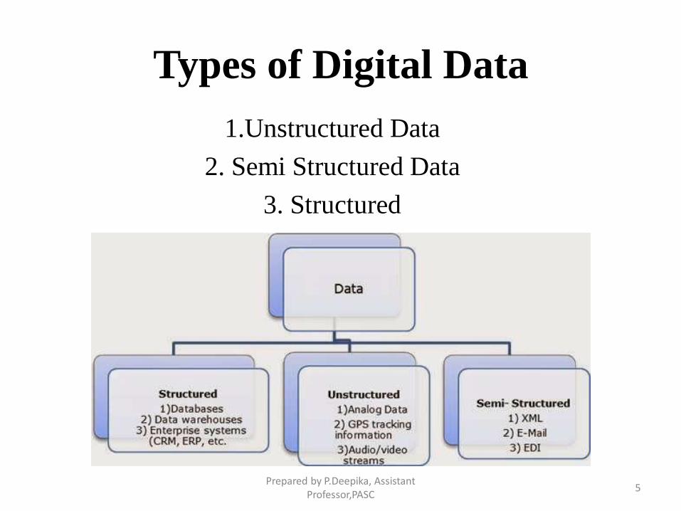
Types of Digital Data

1.Unstructured Data

2. Semi Structured Data

3. Structured


5

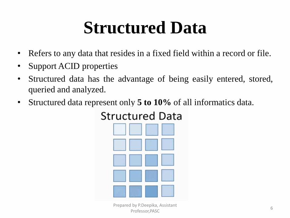
Structured Data

• Refers to any data that resides in a fixed field within a record or file.

• Support ACID properties

• Structured data has the advantage of being easily entered, stored,

queried and analyzed.

• Structured data represent only 5 to 10% of all informatics data.


6

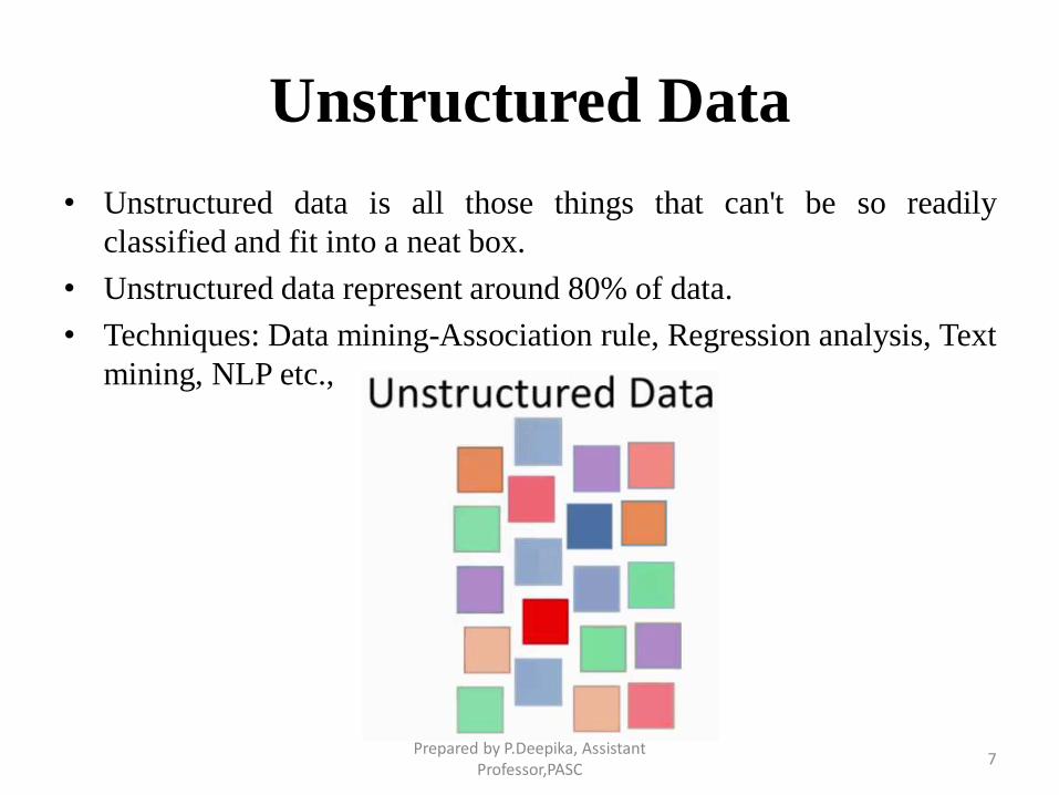
Unstructured Data

• Unstructured data is all those things that can't be so readily

classified and fit into a neat box.

• Unstructured data represent around 80% of data.

• Techniques: Data mining-Association rule, Regression analysis, Text

mining, NLP etc.,


7

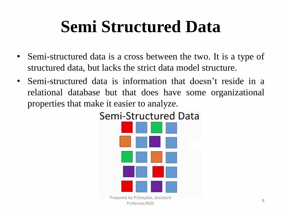
Semi Structured Data

• Semi-structured data is a cross between the two. It is a type of

structured data, but lacks the strict data model structure.

• Semi-structured data is information that doesn’t reside in a

relational database but that does have some organizational

properties that make it easier to analyze.


8

Characteristic of Data

• Composition - What is the Structure, type and Nature

of data?

• Condition - Can the data be used as it is or it needs to

be cleansed?

• Context - Where this data is generated? Why? How

sensitive this data? What are the events associated

with this data?


9

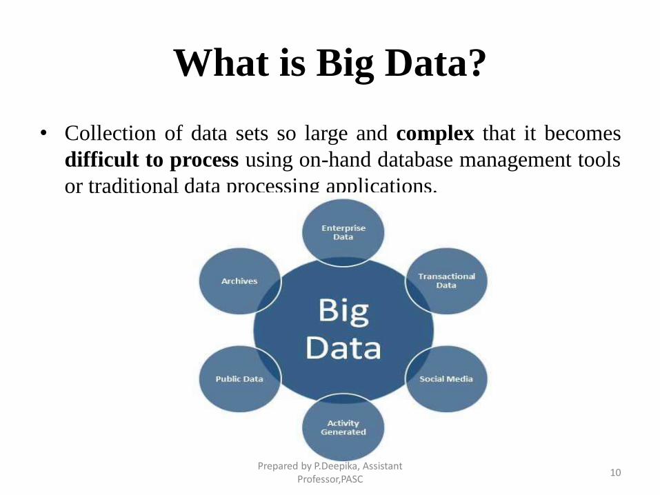
What is Big Data?

• Collection of data sets so large and complex that it becomes

difficult to process using on-hand database management tools

or traditional data processing applications.


10

What is Big Data?

• The data is too big, moves too fast, or doesn’t fit the structures

of your database architectures

• The scale, diversity, and complexity of the data require new

architecture, techniques, algorithms, and analytics to manage it

and extract value and hidden knowledge from it

• Big data is the realization of greater business intelligence by

storing, processing, and analyzing data that was previously

ignored due to the limitations of traditional data management

technologies.


11

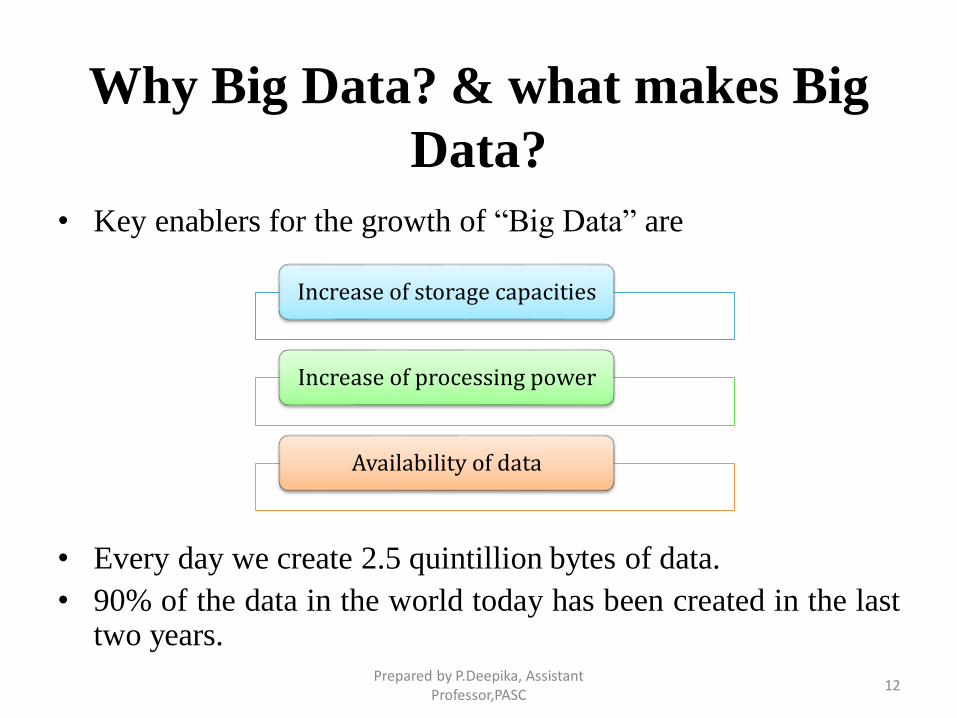
Why Big Data? & what makes Big

Data?

• Key enablers for the growth of “Big Data” are

• Every day we create 2.5 quintillion bytes of data.

• 90% of the data in the world today has been created in the lasttwo years.

Increase of storage capacities

Increase of processing power

Availability of data


12

Where does data come from?

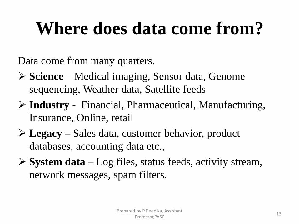
Data come from many quarters.

Science – Medical imaging, Sensor data, Genome

sequencing, Weather data, Satellite feeds

Industry - Financial, Pharmaceutical, Manufacturing,

Insurance, Online, retail

Legacy – Sales data, customer behavior, product

databases, accounting data etc.,

System data – Log files, status feeds, activity stream,

network messages, spam filters.


13

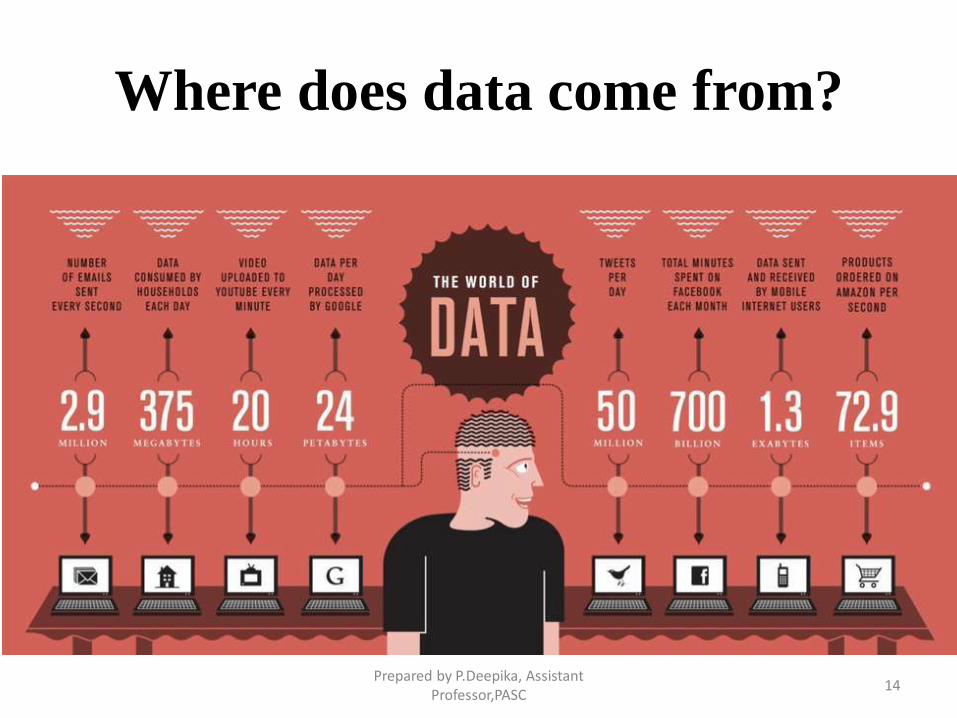
Where does data come from?


14

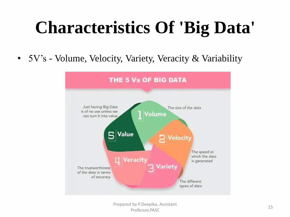
Characteristics Of 'Big Data'

• 5V’s - Volume, Velocity, Variety, Veracity & Variability


15

CHALLENGES

• More data = more storage space

• Data coming faster

• Needs to handle various data structure

• Agile business requirement

• Securing big data

• Data consistency & quality


16

What is the importance of Big Data?

• The importance of big data is how you utilize the data which

you own. Data can be fetched from any source and analyze it

to solve that enable us in terms of

1) Cost reductions

2) Time reductions

3) New product development and optimized offerings, and

4) Smart decision making.


17

What is the importance of Big Data?

• Combination of big data with high-powered analytics, you can

have great impact on your business strategy such as:

1) Finding the root cause of failures, issues and defects in real

time operations.

2) Generating coupons at the point of sale seeing the customer’s

habit of buying goods.

3) Recalculating entire risk portfolios in just minutes.

4) Detecting fraudulent behavior before it affects and risks your

organization.


18

Who are the ones who use the Big

Data Technology?

• Banking

• Government

• Education

• Health Care

• Manufacturing

• Retail


19

Storing Big Data

• Analyzing your data characteristics

Selecting data sources for analysis

Eliminating redundant data

Establishing the role of NoSQL

• Overview of Big Data stores

Data models: key value, graph, document,

column-family

Hadoop Distributed File System

HBase

Hive


20

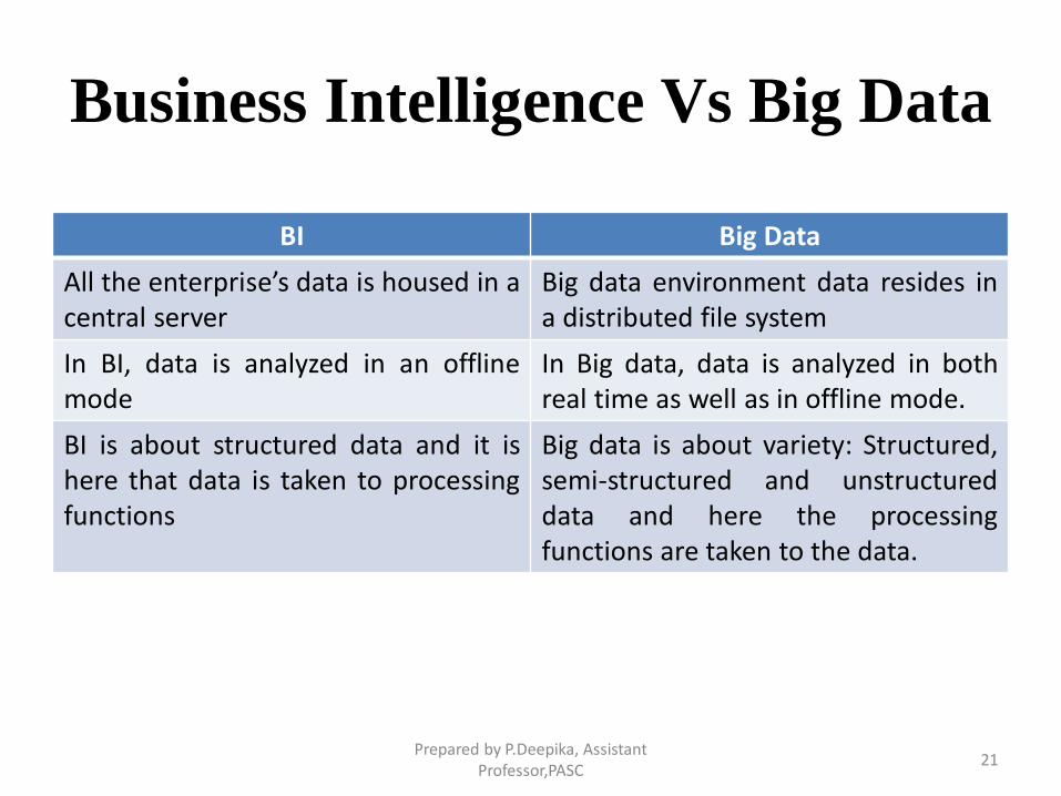
Business Intelligence Vs Big Data

BI Big Data

All the enterprise’s data is housed in acentral server

Big data environment data resides ina distributed file system

In BI, data is analyzed in an offlinemode

In Big data, data is analyzed in bothreal time as well as in offline mode.

BI is about structured data and it ishere that data is taken to processingfunctions

Big data is about variety: Structured,semi-structured and unstructureddata and here the processingfunctions are taken to the data.


21

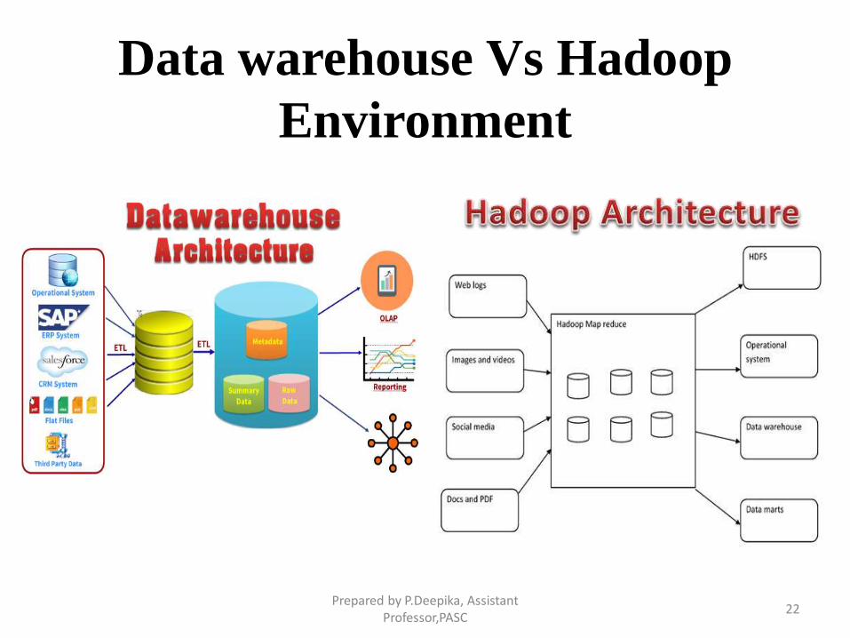
Data warehouse Vs Hadoop

Environment


22

UNIT II


23

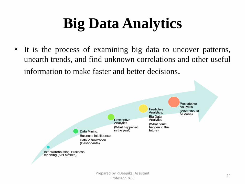
Big Data Analytics

• It is the process of examining big data to uncover patterns,

unearth trends, and find unknown correlations and other useful

information to make faster and better decisions.


24

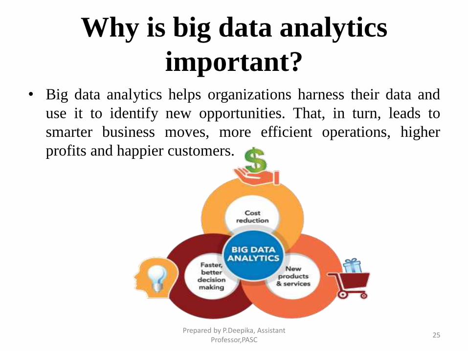
Why is big data analytics

important?• Big data analytics helps organizations harness their data and

use it to identify new opportunities. That, in turn, leads to

smarter business moves, more efficient operations, higher

profits and happier customers.


25

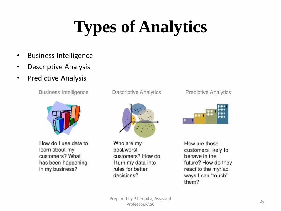
Types of Analytics

• Business Intelligence

• Descriptive Analysis

• Predictive Analysis


26

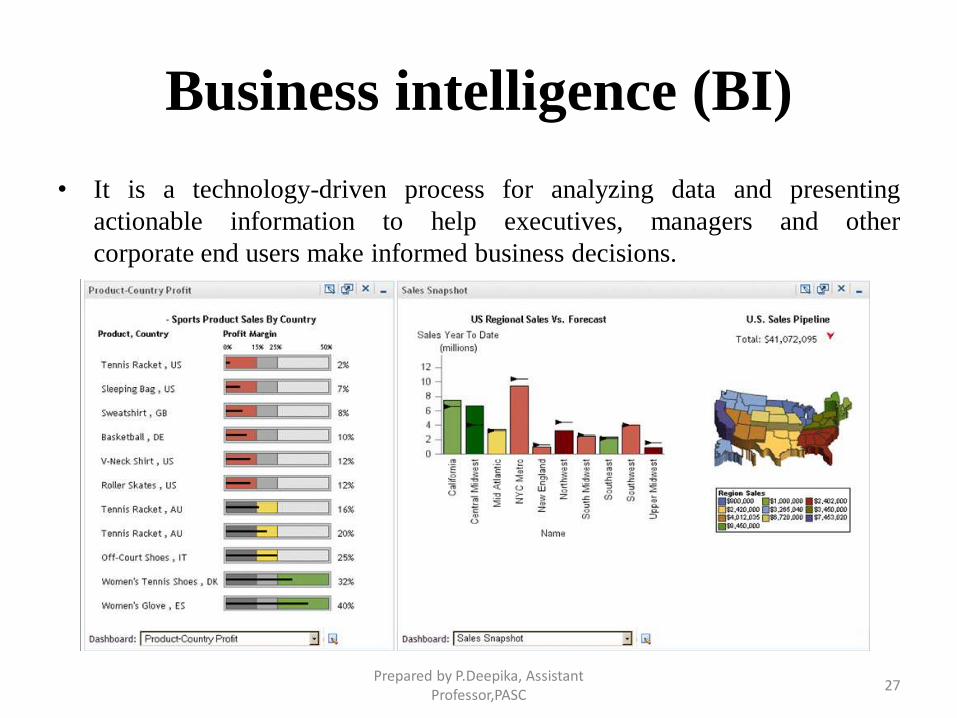
Business intelligence (BI)

• It is a technology-driven process for analyzing data and presenting

actionable information to help executives, managers and other

corporate end users make informed business decisions.


27

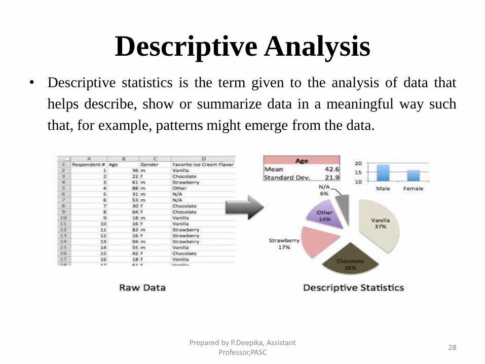
Descriptive Analysis• Descriptive statistics is the term given to the analysis of data that

helps describe, show or summarize data in a meaningful way such

that, for example, patterns might emerge from the data.


28

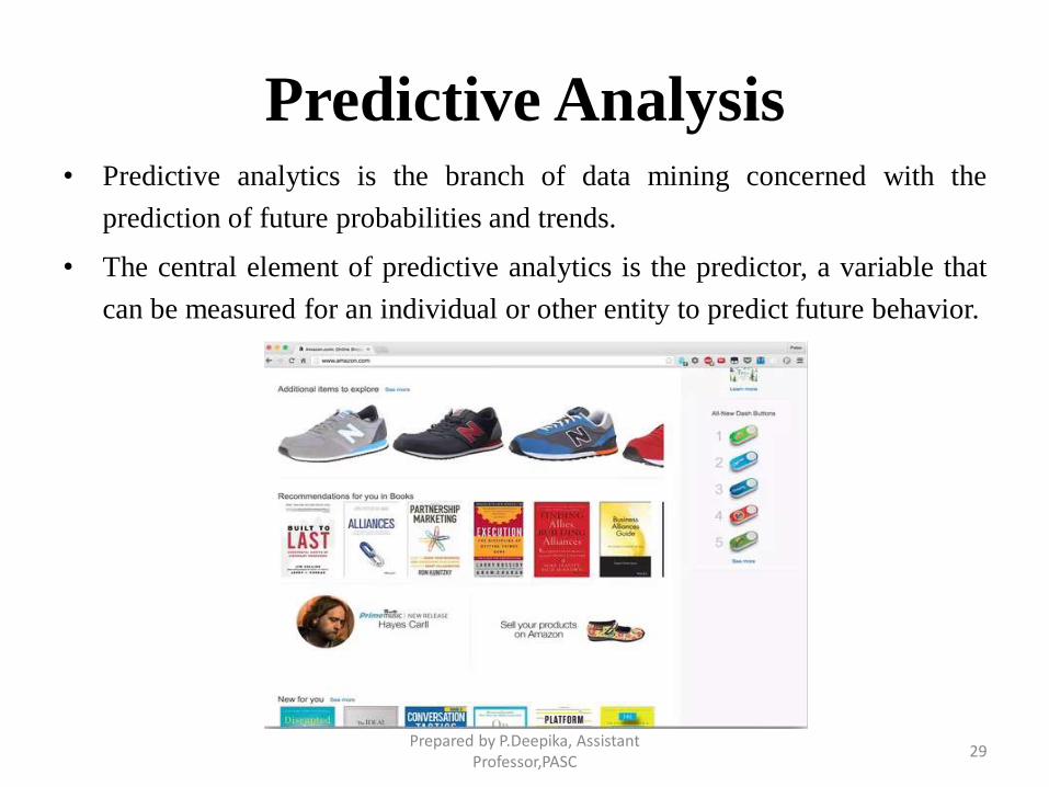
Predictive Analysis• Predictive analytics is the branch of data mining concerned with the

prediction of future probabilities and trends.

• The central element of predictive analytics is the predictor, a variable that

can be measured for an individual or other entity to predict future behavior.


29

Predictive Analysis

• There is 2 types of predictive analytics:

◦ Supervised

Supervised analytics is when we know the truth about

something in the past

Example: We have historical weather data. The temperature,

humidity, cloud density and weather type (rain, cloudy, or sunny). Then we can

predict today weather based on temp, humidity, and cloud density today

◦ Unsupervised

Unsupervised is when we don’t know the truth about

something in the past. The result is segment that we need to interpret

Example: We want to do segmentation over the student

based on the historical exam score, attendance, and late history.


30

Big Data Analytics

• Large volume of unstructured data, which cannot be handled

by standard database management systems like

DBMS,RDBMS or ORDBMS

• High volume/High Variety/High Velocity information assets

require new forms of processing/analytics to enable enhanced

decision making, insight discovery and optimization


31

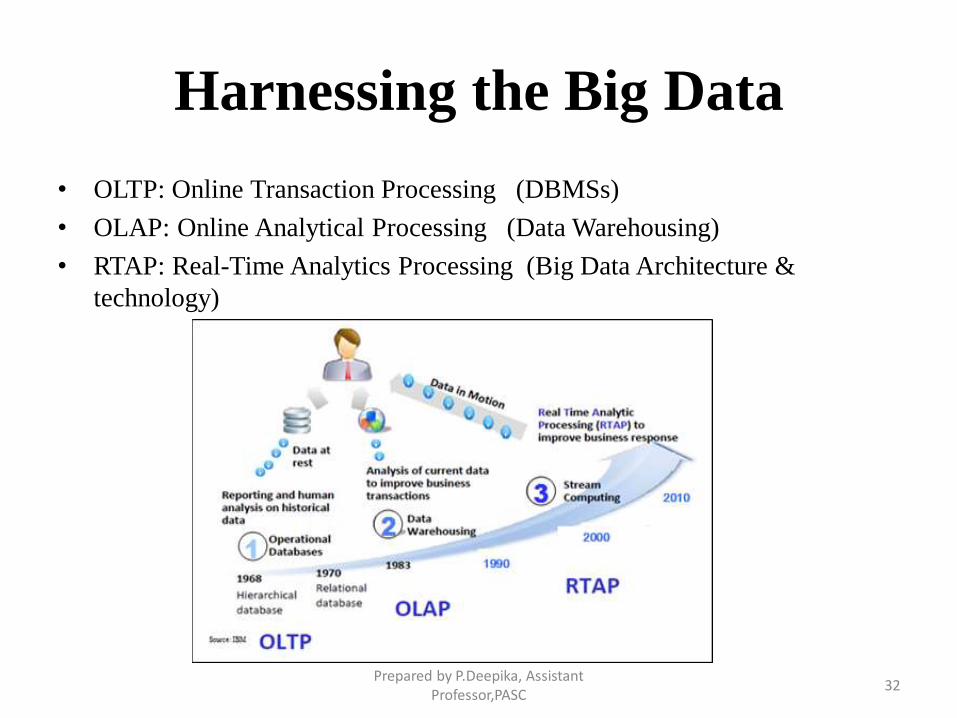
Harnessing the Big Data

• OLTP: Online Transaction Processing (DBMSs)

• OLAP: Online Analytical Processing (Data Warehousing)

• RTAP: Real-Time Analytics Processing (Big Data Architecture &

technology)


32

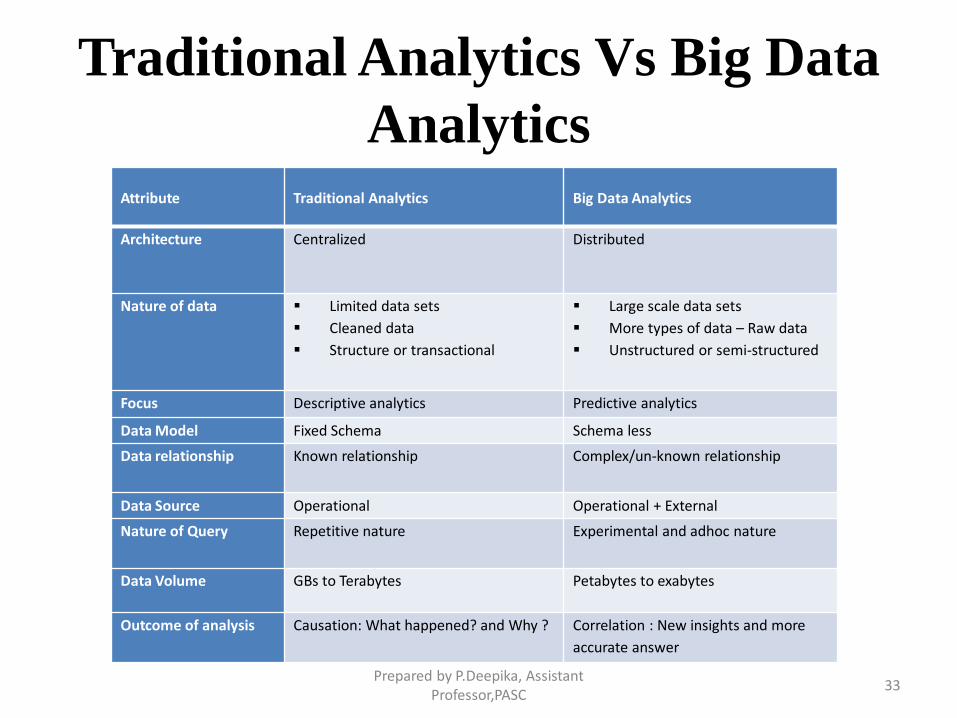
Traditional Analytics Vs Big Data

AnalyticsAttribute Traditional Analytics Big Data Analytics

Architecture Centralized Distributed

Nature of data Limited data sets

Cleaned data

Structure or transactional

Large scale data sets

More types of data – Raw data

Unstructured or semi-structured

Focus Descriptive analytics Predictive analytics

Data Model Fixed Schema Schema less

Data relationship Known relationship Complex/un-known relationship

Data Source Operational Operational + External

Nature of Query Repetitive nature Experimental and adhoc nature

Data Volume GBs to Terabytes Petabytes to exabytes

Outcome of analysis Causation: What happened? and Why ? Correlation : New insights and more

accurate answer


33

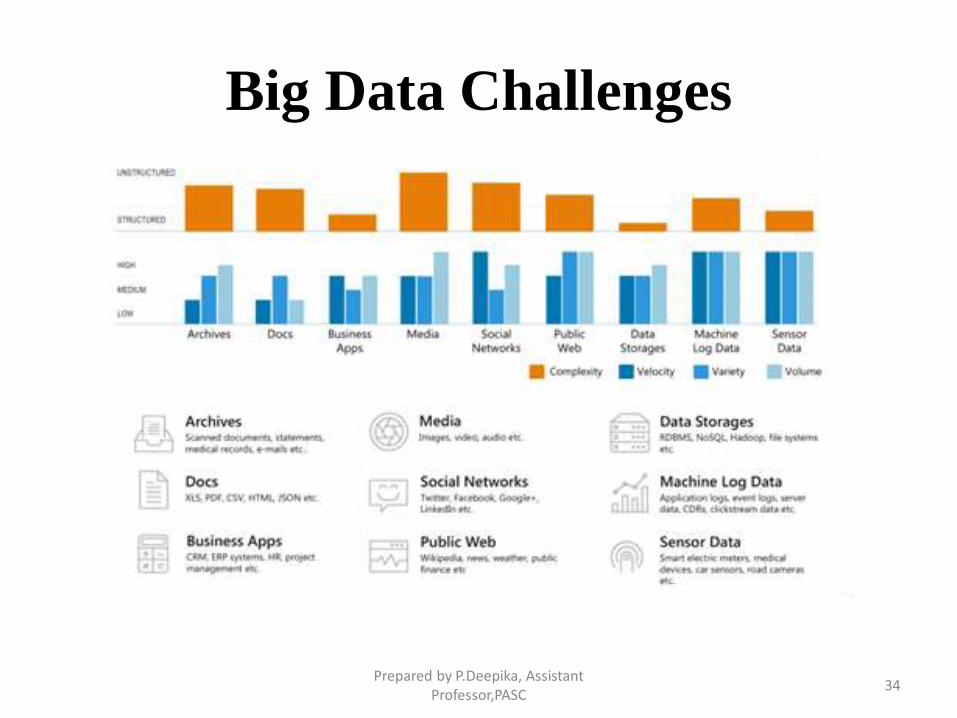
Big Data Challenges


34

Value of Big Data Analytics &

Challenges

• Big data is more real-time in nature than traditional/ DW

applications

• Traditional DW architectures are not well-suited for big data

applications

• Shared nothing, massively parallel processing, scale out

architectures are well-suited for big data applications

• New architecture, algorithms, techniques are needed


35

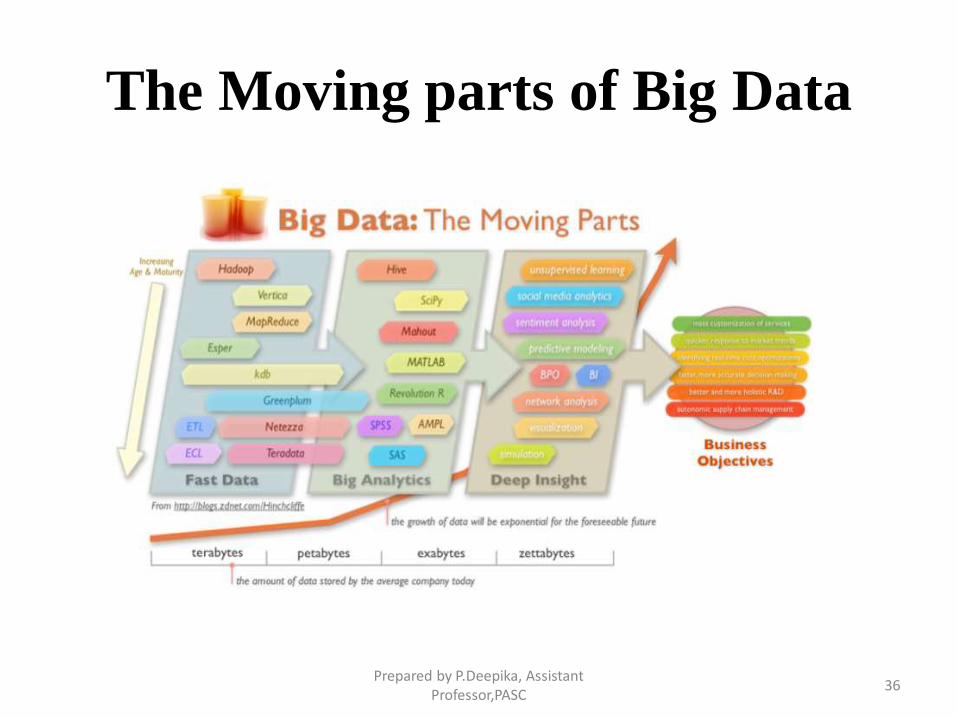
The Moving parts of Big Data


36

Top Big Data Technologies

1. Apache Hadoop

• Apache Hadoop is a java based free software framework that can

effectively store large amount of data in a cluster.

• Hadoop Distributed File System (HDFS) is the storage system of Hadoop

which splits big data and distribute across many nodes in a cluster.

• This also replicates data in a cluster thus providing high availability. It uses

Map Reducing algorithm for processing.


37


2. NoSQL• NoSQL (Not Only SQL)is used to handle unstructured data.

• NoSQL databases store unstructured data with no particular schema.

• NoSQL gives better performance in storing massive amount of data. There

are many open-source NoSQL DBs available to analyse big Data.


38


3. Apache Spark

• Apache Spark is part of the Hadoop ecosystem, but its use has

become so widespread that it deserves a category of its own.

• It is an engine for processing big data within Hadoop, and it's

up to one hundred times faster than the standard Hadoop

engine, Map Reduce.


39


4. R

• R, another open source project, is a programming language

and software environment designed for working with statistics.

• Many popular integrated development environments (IDEs),

including Eclipse and Visual Studio, support the language.


40

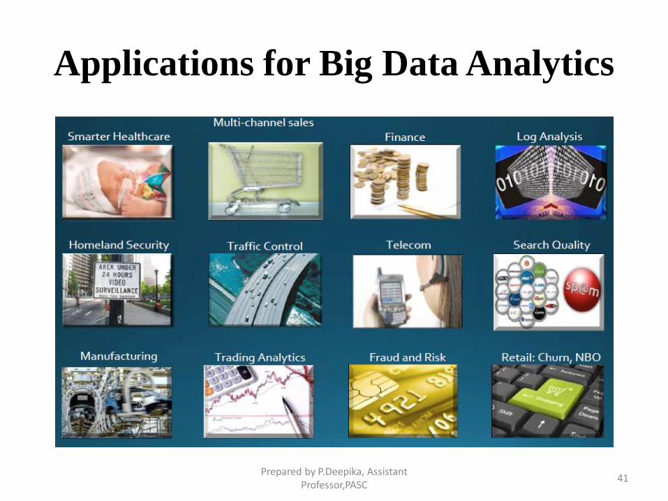
Applications for Big Data Analytics


41

Data Science

• Data science is the science of extracting knowledge from data.

• It is a science of drawing out hidden patterns amongst data

using statistical and mathematical techniques.

• It employs techniques and theories drawn from many fields

from the broad areas of mathematics, statistics, information

technology including machine learning, data engineering,

probability models, statistical learning, pattern recognition etc.


42

Business Acumen Skills

• The following is the list of traits that needs to be honed to play

the role of data scientist.

Understanding of domain

Business strategy

Problem solving

Communication

Presentation

Inquisitiveness


43

Technology Expertise

• Listed below are the few skills required as far as technical

expertise is concerned.

Good database knowledge such as RDBMS.

Good NoSQL database knowledge such as MongoDB,

Cassandra, HBase, etc.

Programming languages such as Java, Python, C++, etc.

Open source tools such as Hadoop.

Data warehousing

Data mining

Visualization such as Tableau, Flare, Google Visualization

APIs, etc.


44

Mathematical Expertise

• Following are the key skills a data scientist should have in his

arsenal.

Mathematics

Statistics

Artificial Intelligence

Algorithms

Machine Learning

Pattern Recognition

Natural Language Processing


45

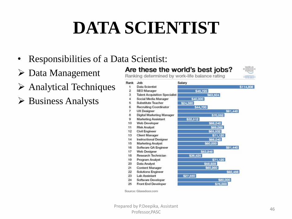
DATA SCIENTIST

• Responsibilities of a Data Scientist:

Data Management

Analytical Techniques

Business Analysts


46

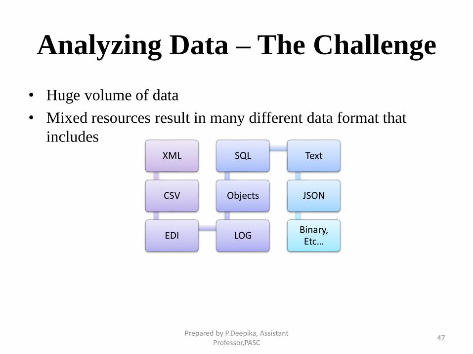
Analyzing Data – The Challenge

• Huge volume of data

• Mixed resources result in many different data format that

includesXML

CSV

EDI LOG

Objects

SQL Text

JSON

Binary, Etc…


47

Analyzing Data with Hadoop

• Batch processing

• Parallel execution

• Spread data over a cluster of servers and take the computation

to the data

– Analysis conducted at lower cost

– Analysis conducted in less time

– Greater flexibility

– Linear scalability


48

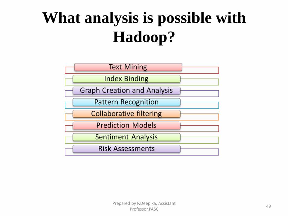
What analysis is possible with

Hadoop?


49

Modeling true risk

• Challenge:

– How much risk exposure does an organization really have

with each customer?

• Solution with the Hadoop:

– Source and aggregate disperse data sources to build data

picture – eg. Credit card records, call recordings, chat

sessions, e-mails, banking activity

– Structure and analysis – Sentiment analysis, graph creation,

pattern recognition

• Typical Industry:

– Financial services - Bank, insurance companies


50

Customer Churn Analysis• Challenge:

– Why organizations are really losing customer?


– Rapidly build behavioral model from disparate data sources

– Structure and analyze with Hadoop – Traversing, Graph creation, pattern

recognition


– Telecommunication, Financial Services

• Recommending Engine / Ad targeting

• Challenge:

– Using user data to predict which products to recommend


– Batch processing framework – Allow execution in parallel over large data sets

– Collaborative filtering – Collect taste information from many users and

utilizing information to predict what similar users like


– E-Commerce, Manufacturing, Retail, Advertising Prepared by P.Deepika, Assistant

Professor,PASC51

Point of sale transaction analysis

• Challenge:

– Analyzing Point of Sale (PoS) data to target promotions

and manage operations

– Sources are complex and data volumes grow across chains

of stores and other sources


– Batch processing framework – Allow execution in parallel

over large data sets

• Pattern recognition

• Optimizing over multiple data sources

• Utilizing information to predict demand


52


– Retail

• Challenge:

– Analyzing real-time data series from network of sensors

– Calculating average frequency over time is extremely tedious

because of the need to analyze terabytes


– Task the computation to the data

– Expand from simple scans to more complex data mining

– Better understand how the network reacts to fluctuations

– Discrete anomalies may, in fact, be interconnected

– Identify the leading indicators of component failure


53


– Telecommunication, Data centers

• Threat Analysis / Trade Surveillance

• Challenge:

– Detecting threats in the form of fraudulent activity or attacks

• Large data volumes involved

• Like looking of needle in a hay stack


– Parallel processing over huge data sets

– Pattern recognition to identify anomalies – eg. Threats


– Security, Financial services,

– General – Spam fighting, Click fraud


54

Search Quality

• Challenge:

– Providing meaningful search results

• Solution with the Hadoop

– Analyzing search attempts in conjunction with structured

data

• Pattern recognition

– Browsing pattern of users performing searches in different

categories

• Typical Industry

• Web, E-Commerce


55

Data Sand Box

• Challenge:

– Data Deluge - Don’t know what to do with the data or what

analysis to run


– “Dump” all this data into an HDFS cluster

– Use Hadoop to start trying out different analysis on the data

– See patterns to derive value from data


– Common across all Industries


56

Terminologies used in Big Data

Environments

• In-Memory Analytics:

– All the relevant data is stored in RAM or primary storage thus

eliminating the need to access data from hard disk.

• In-Database Processing:

– It works by fusing data warehouses with analytical systems.

• Massively Parallel Processing (MPP):

– It is a coordinated processing of programs by a number of processors

working in parallel.

– Each processor has its own OS and dedicated memory.

– MPP processors communicate using message interfaces.


57

Terminologies used in Big Data

Environments

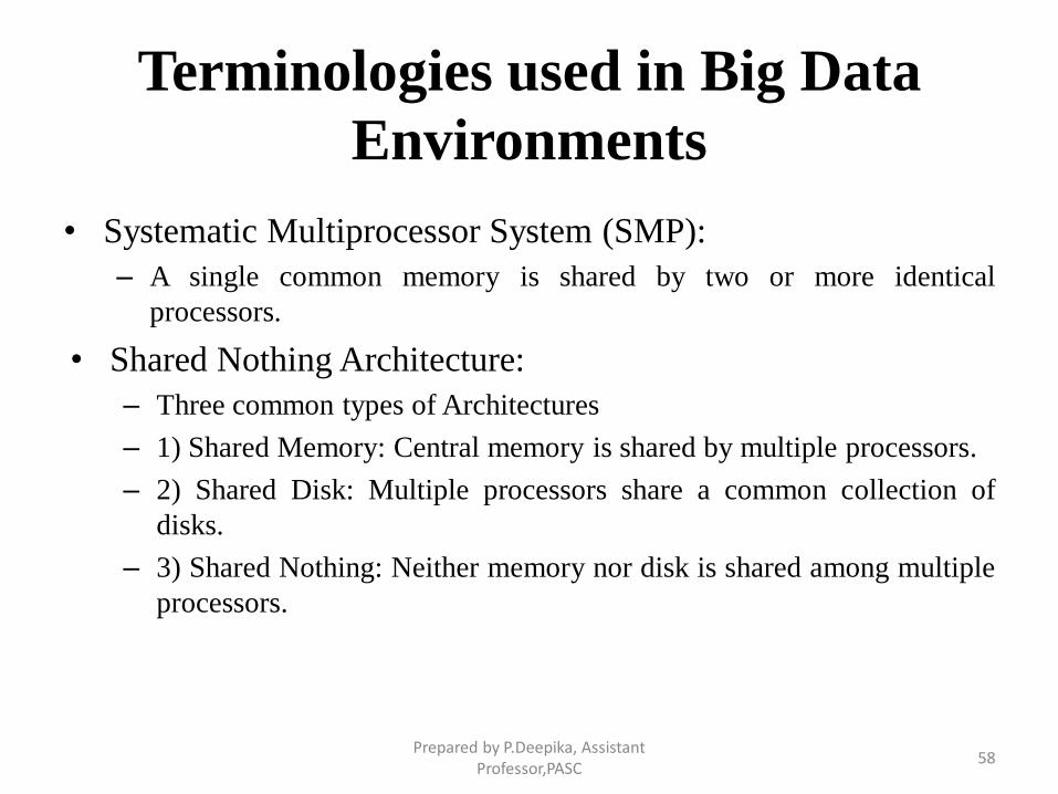
• Systematic Multiprocessor System (SMP):

– A single common memory is shared by two or more identical

processors.

• Shared Nothing Architecture:

– Three common types of Architectures

– 1) Shared Memory: Central memory is shared by multiple processors.

– 2) Shared Disk: Multiple processors share a common collection of

disks.

– 3) Shared Nothing: Neither memory nor disk is shared among multiple

processors.


58

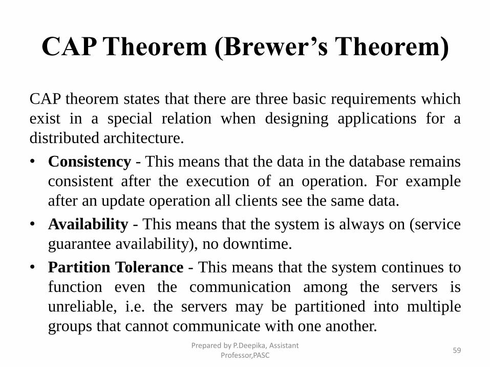
CAP Theorem (Brewer’s Theorem)

CAP theorem states that there are three basic requirements which

exist in a special relation when designing applications for a

distributed architecture.

• Consistency - This means that the data in the database remains

consistent after the execution of an operation. For example

after an update operation all clients see the same data.

• Availability - This means that the system is always on (service

guarantee availability), no downtime.

• Partition Tolerance - This means that the system continues to

function even the communication among the servers is

unreliable, i.e. the servers may be partitioned into multiple

groups that cannot communicate with one another.Prepared by P.Deepika, Assistant

Professor,PASC59

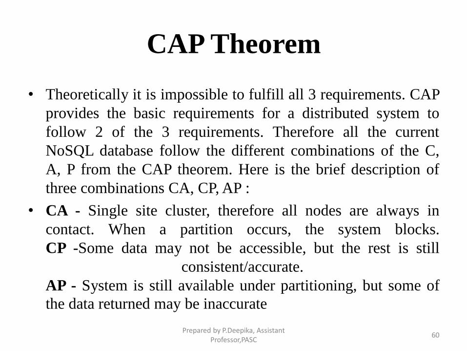
CAP Theorem

• Theoretically it is impossible to fulfill all 3 requirements. CAP

provides the basic requirements for a distributed system to

follow 2 of the 3 requirements. Therefore all the current

NoSQL database follow the different combinations of the C,

A, P from the CAP theorem. Here is the brief description of

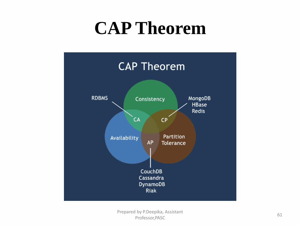
three combinations CA, CP, AP :

• CA - Single site cluster, therefore all nodes are always in

contact. When a partition occurs, the system blocks.

CP -Some data may not be accessible, but the rest is still

consistent/accurate.

AP - System is still available under partitioning, but some of

the data returned may be inaccurate


60

CAP Theorem


61

• BASE:– Basically Available Soft State Eventual Consistency

(BASE) is used in distributed computing to achieve highavailability.

• Few Analytical Tools:MS Excel

SAS

IBM SPSS Modeler

Statistica

Salford systems

WPS

• Open Source Analytics Tools:R analysis

Weka


62

UNIT III


63

ACID Rules

A database transaction, must be atomic, consistent, isolated and durable.

Below we have discussed these four points.

• Atomic : A transaction is a logical unit of work which must be either

completed with all of its data modifications, or none of them is performed.

• Consistent : At the end of the transaction, all data must be left in a

consistent state.

• Isolated : Modifications of data performed by a transaction must be

independent of another transaction. Unless this happens, the outcome of a

transaction may be erroneous.

• Durable : When the transaction is completed, effects of the modifications

performed by the transaction must be permanent in the system.


64

Distributed Systems

• A distributed system consists of multiple computers and

software components that communicate through a computer

network (a local network or by a wide area network).

• A distributed system can consist of any number of possible

configurations, such as mainframes, workstations, personal

computers, and so on.

• The computers interact with each other and share the resources

of the system to achieve a common goal.


65

Advantages of Distributed

Computing

• Reliability (fault tolerance)

• Scalability

• Sharing of Resources

• Flexibility

• Speed

• Open system

• Performance


66

Disadvantages of Distributed

Computing

• Troubleshooting

• Software

• Networking

• Security


67

What is NoSQL?

• NoSQL is a non-relational database management systems,

different from traditional relational database management

systems in some significant ways.

• It is designed for distributed data stores where very large scale

of data storing needs (for example Google or Facebook which

collects terabits of data every day for their users).

• These type of data storing may not require fixed schema, avoid

join operations and typically scale horizontally.

• They do not acquire ACID properties.


68

Why NoSQL?

• In today’s time data is becoming easier to access and capture

through third parties such as Facebook, Google+ and others.

Personal user information, social graphs, geo location data,

user-generated content and machine logging data are just a few

examples where the data has been increasing exponentially.

• To avail the above service properly, it is required to process

huge amount of data. Which SQL databases were never

designed.

• The evolution of NoSql databases is to handle these huge data

properly.


69

Example

• Social-network graph:

– Each record: UserID1, UserID2

– Separate records: UserID, first_name,last_name, age, gender,...

– Task: Find all friends of friends of friends of ... friends of a given user.

• Wikipedia pages :

– Large collection of documents

– Combination of structured and unstructured data

– Task: Retrieve all pages regarding athletics of Summer Olympic before

1950.


70

RDBMS Vs NoSQL

• RDBMS - Structured and organized data - Structured query language (SQL) - Data and its relationships are stored in separate tables. - Data Manipulation Language, Data Definition Language - Tight Consistency

• NoSQL- Stands for Not Only SQL- No declarative query language- No predefined schema - Key-Value pair storage, Column Store, Document Store, Graph databases- Eventual consistency rather ACID property - Unstructured and unpredictable data- CAP Theorem - Prioritizes high performance, high availability and scalability- BASE Transaction


71

NoSQL Categories

• There are four general types (most common categories) of

NoSQL databases. Each of these categories has its own

specific attributes and limitations. There is not a single

solutions which is better than all the others, however there are

some databases that are better to solve specific problems.

Key-value stores

Column-oriented

Graph

Document oriented


72

Key-value stores

• Key-value stores are most basic types of NoSQL databases.

• Designed to handle huge amounts of data.

• Based on Amazon’s Dynamo paper.

• Key value stores allow developer to store schema-less data.

• In the key-value storage, database stores data as hash table where each key is

unique and the value can be string, JSON, BLOB (Binary Large OBjec) etc.

• A key may be strings, hashes, lists, sets, sorted sets and values are stored against

these keys.

• For example a key-value pair might consist of a key like "Name" that is associated

with a value like "Robin".

• Key-Value stores can be used as collections, dictionaries, associative arrays etc.

• Key-Value stores follow the 'Availability' and 'Partition' aspects of CAP theorem.

• Key-Values stores would work well for shopping cart contents, or individual values

like color schemes, a landing page URI, or a default account number.


73

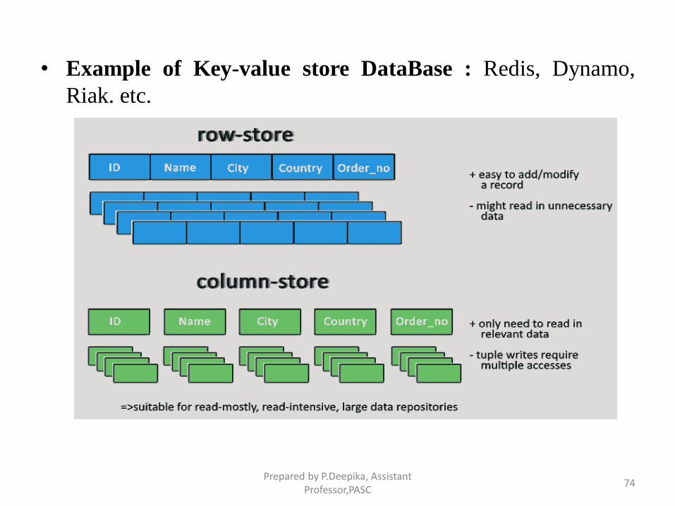
• Example of Key-value store DataBase : Redis, Dynamo,

Riak. etc.


74


75

Column-oriented databases

• Column-oriented databases primarily work on columns and every column

is treated individually.

• Values of a single column are stored contiguously.

• Column stores data in column specific files.

• In Column stores, query processors work on columns too.

• All data within each column datafile have the same type which makes it

ideal for compression.

• Column stores can improve the performance of queries as it can access

specific column data.

• High performance on aggregation queries (e.g. COUNT, SUM, AVG, MIN,

MAX).

• Works on data warehouses and business intelligence, customer relationship

management (CRM), Library card catalogs etc.


76

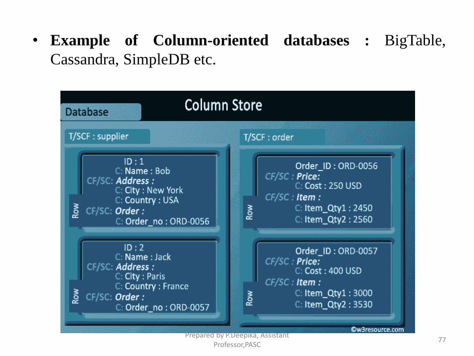
• Example of Column-oriented databases : BigTable,

Cassandra, SimpleDB etc.


77

Graph databases

• A graph data structure consists of a finite (and possibly mutable) set ofordered pairs, called edges or arcs, of certain entities called nodes orvertices.

• The following picture presents a labeled graph of 6 vertices and 7 edges.

• A graph database stores data in a graph.

• It is capable of elegantly representing any kind of data in a highlyaccessible way.

• A graph database is a collection of nodes and edges

• Each node represents an entity (such as a student or business) and eachedge represents a connection or relationship between two nodes.

• Every node and edge are defined by a unique identifier.

• Each node knows its adjacent nodes.

• As the number of nodes increases, the cost of a local step (or hop) remainsthe same.

• Index for lookups.


78

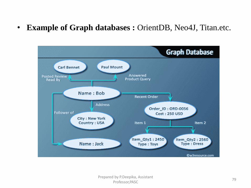
• Example of Graph databases : OrientDB, Neo4J, Titan.etc.


79

Document Oriented databases

• A collection of documents

• Data in this model is stored inside documents.

• A document is a key value collection where the key allows

access to its value.

• Documents are not typically forced to have a schema and

therefore are flexible and easy to change.

• Documents are stored into collections in order to group

different kinds of data.

• Documents can contain many different key-value pairs, or key-

array pairs, or even nested documents.


80

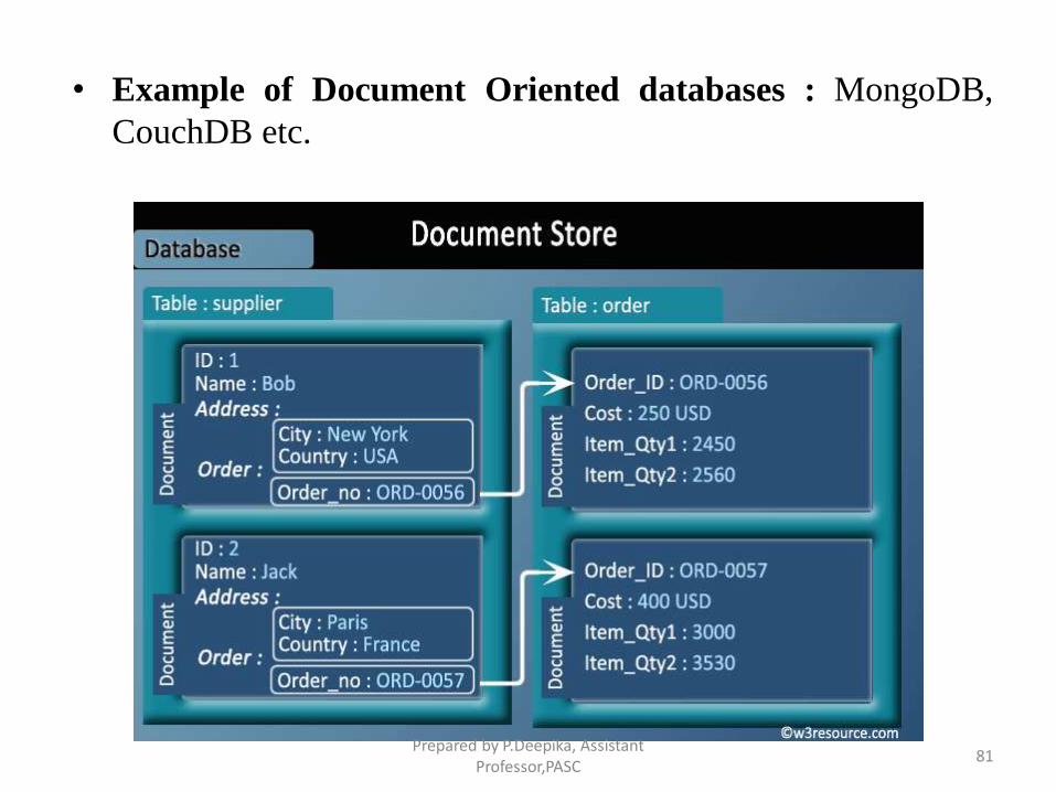
• Example of Document Oriented databases : MongoDB,

CouchDB etc.


81

NoSQL pros/cons

Advantages :

• High scalability

• Distributed Computing

• Lower cost

• Schema flexibility, semi-structure data

• No complicated Relationships

Disadvantages

• No standardization

• Limited query capabilities (so far)


82

Popular NoSQL Databases


83

http://www.tutorialspoint.com/articles/wp-content/uploads/2015/09/nosql_databases.png

http://www.tutorialspoint.com/articles/wp-content/uploads/2015/09/nosql_databases.png

NewSQL

• NewSQL overcomes the drawbacks of NoSQL and acquires

the advantage of SQL.

• It has the same scalable performance of NoSQL systems for

On Line Transaction processing (OLTP) while maintaining the

ACID properties of a traditional database.


84

HADOOP

• Hadoop is a distributed file system and data processing engine thatis designed to handle extremely high volumes of data in anystructure.

• An open-source software framework that supports data-intensivedistributed applications, licensed under the Apache v2 license.

• A flexible, scalable and highly-available architecture for large scalecomputation and data processing on a network of commodityhardware

• Abstract and facilitate the storage and processing of large and / orrapidly growing data sets of structured and non-structured data usingsimple programming models.

• Designed to answer the question: “How to process big data withreasonable cost and time?”

• A large and an active ecosystem


85

How Hadoop meets Big Data

Analytics?

• “Big data” creates large business values today

• $10.2 billion worldwide revenue from big data analytics in

2013

• Many firms end up creating large amount of data that they are

unable to gain any insight from it

• Without an efficient data processing approach, the data cannot

create business values.

• Hadoop addresses “big data” challenges


86

Hadoop – Components

• Hadoop has two components :

– The Hadoop distributed File System (HDFS) – which

supports data in structured relational form, in unstructured

form, any in any form in between

– The MapReduce programming paradigm - for managing

applications on multiple distributed servers

• There are many other projects based around core Hadoop

– Often referred to as ” Hadoop Eco System” - Pig, Hive,

HBase, Flume, Oozie, Sqoop, Mahout , etc.,


87

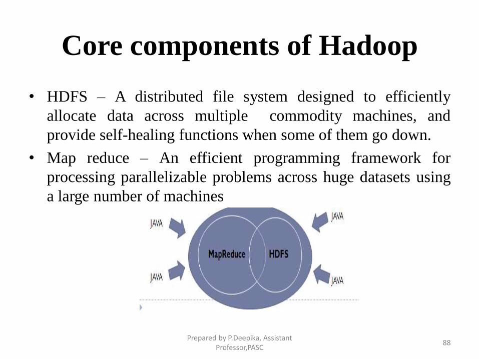
Core components of Hadoop

• HDFS – A distributed file system designed to efficiently

allocate data across multiple commodity machines, and

provide self-healing functions when some of them go down.

• Map reduce – An efficient programming framework for

processing parallelizable problems across huge datasets using

a large number of machines


88

Hadoop – Assumptions

• Hardware will fail

• Processing will be run in batches.

• Applications that run on HDFS have large data sets.

• Applications need a write-once-read-many access model

• Portability and Scalability for efficient data processing

• Moving Computation is Cheaper than Moving Data


89

Hadoop – Advantages

• Scalable: It can reliably store and process petabytes

• Economical: It distributes the data and processing across

clusters of commonly available computers (in thousands)

• Efficient: By distributing the data, it can process it in parallel

on the nodes where the data is located

• Reliable: It automatically maintains multiple copies of data

and automatically redeploys computing tasks based on failures


90

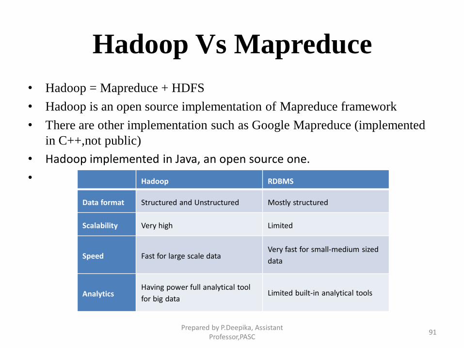
Hadoop Vs Mapreduce

• Hadoop = Mapreduce + HDFS

• Hadoop is an open source implementation of Mapreduce framework

• There are other implementation such as Google Mapreduce (implemented

in C++,not public)

• Hadoop implemented in Java, an open source one.

• Hadoop RDBMS

Data format Structured and Unstructured Mostly structured

Scalability Very high Limited

Speed Fast for large scale data Very fast for small-medium sized

data

Analytics Having power full analytical tool

for big data Limited built-in analytical tools


91

Hadoop Vs RDBMS

• Many businesses are turning from RDBMS to Hadoop based

system for data management.

• If businesses need to process and analyze large-scale, real-time

data, then choose Hadoop. Otherwise staying with RDBMS is

still a wise choice


92

Hadoop – What does it do?

• Hadoop implements Google’s Map Reduce, using HDFS

• Map Reduce divides applications into many small blocks of

work

• HDFS creates multiple replicas of data blocks for reliability,

placing them on compute nodes around the cluster

• Map Reduce can then process the data where it is located

• Hadoop ‘s target is to run on clusters of the order of 10,000-

nodes


93

History of HADOOP

• Hadoop was created by the Dough Cutting, the creator of Apache Lucene –

the widely used text search history

• 2002- Doug Cutting and Michael J. Cafarella, started an open source “web

search engine project called, “Nutch”

• 2003-Sanjay Ghemawat, Howard Gobioff, and Shun-Tak Leung, of Google

published a paper “The Google File System” called GFS, which was being

used in the Google.

• 2004- Doug Cutting and Michael J. Cafarella, set about writing an open

source implementation, the Nutch Distributed File System (NDFS)

• 2004-Google published a paper “Map reduce : Simplified Data Processing

on Large Cluster”

• 2005- The Nutch developers had working Map reduce implementation in

Nutch. All the major Nutch algorithms have been ported to run using Map

reduce and NDFS.


94

• 2006 - They moved out of Nutch to form an independent subproject of

lucene called Hadoop, and Doug Cutting Joined Yahoo!

• Yahoo! provides a dedicated team and the resources to turn hadoop into a

system of that ran at a web scale.

• 2006 - Yahoo gave the project to Apache Software Foundation.

• 2008 - Hadoop wins Terabyte sort benchmark (sorted 1 TB of data running

on a 910 node clusters in 209 seconds, compared to previous record of 209

seconds)

• 2008–Google reported that its Map reduce implementation sorted 1 TB of

data in 68 seconds

• 2009 –It was announced that a team at Yahoo! sorted 1 TB of data in 62

seconds using Hadoop

• 2010 - Hadoop's Hbase, Hive and Pig subprojects completed, adding more

computational power to Hadoop framework

• 2011 – Zoo Keeper Completed

• 2013 - Hadoop 1.1.2 and Hadoop 2.0.3 alpha. Ambari, Cassandra, Mahout

have been added


95

HDFS

• A distributed Java-based file system for storing large volumes

of data

• Highly fault-tolerant and is designed to be deployed on low-

cost hardware

• Since HDFS is written in Java, designed for portability across

heterogeneous hardware and software platforms

• HDFS is implemented as a user-level file system in java which

exploits the native file system on each node to store data


96

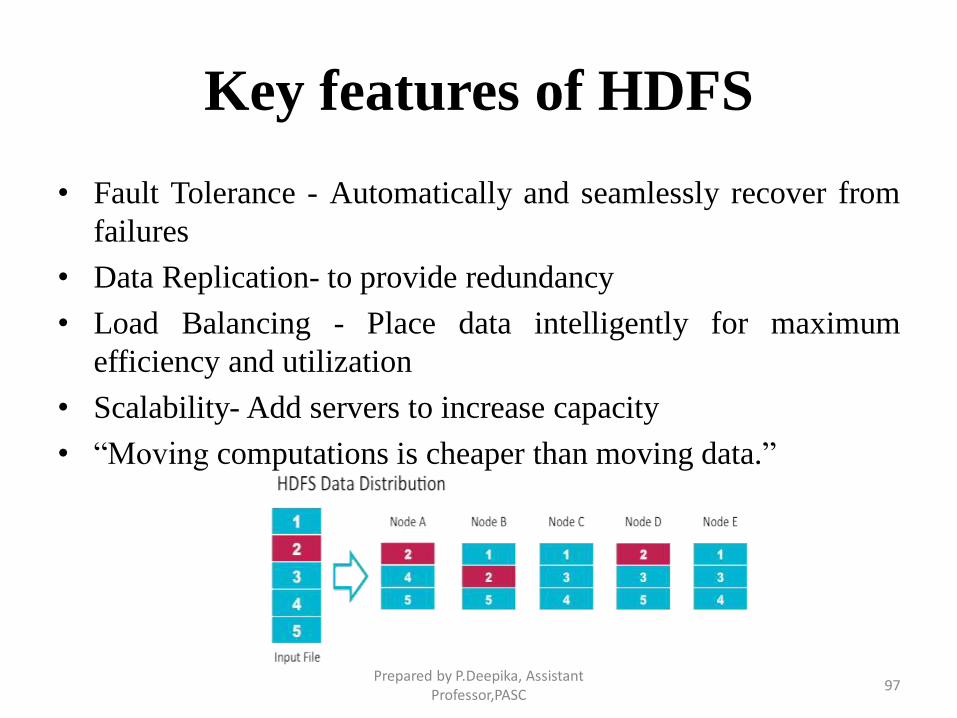
Key features of HDFS

• Fault Tolerance - Automatically and seamlessly recover from

failures

• Data Replication- to provide redundancy

• Load Balancing - Place data intelligently for maximum

efficiency and utilization

• Scalability- Add servers to increase capacity

• “Moving computations is cheaper than moving data.”


97

Hadoop Cluster

• A set of machine running HDFS and Map reduce is known as a

Hadoop cluster

• Individual machines are known as nodes. A cluster can have as

few as one node, as many as several thousands

• More nodes = better performance

• The focus is on supporting redundancy, distributed architecture

and parallel processing

• An important characteristic of Hadoop is the partitioning of

data and computation across many (thousands of hosts, and

executing application computations in parallel)


98

Cluster Specification

• Hadoop is designed to run on commodity hardware.

• Need not tied to expensive, proprietary offerings from a single

vendor

• Provision for choosing commonly available hardware from any of a

large range of vendors to build the cluster

• “Commodity” does not mean “low-end.”

• A typical choice of machine for running a Hadoop Data Node and

Task Tracker would have the following configuration:

• Processor - Two quad-core 2-2.5 GHz CPUs

• Memory - 16-24 GB ECC RAM

• Storage - Four 1 TB SATA disks

• Network - Gigabit Ethernet


99

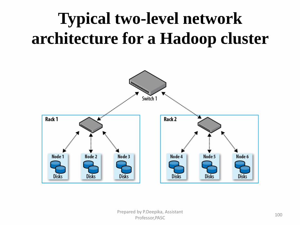
Typical two-level network

architecture for a Hadoop cluster


100

How large a cluster should be?

• One can start with a small cluster (say, 10 nodes) and grow it as your

storage and computational needs grow.

• It is usually acceptable to run the namenode and the jobtracker on a

single master machine

• As the cluster and the number of files stored in HDFS grow, the

namenode needs more memory, so the namenode and jobtracker

should be moved onto separate machines.

• The secondary namenode can be run on the same machine as the

namenode, but again for reasons of memory usage (the secondary

has the same memory requirements as the primary), it is best to run

it on a separate piece of hardware, especially for larger clusters

• Machines running the namenodes should typically run on 64-bit

hardware to avoid the 3 GB limit on Java heap size in 32-bit

architectures.Prepared by P.Deepika, Assistant

Professor,PASC101

Network Topology

• A common Hadoop cluster architecture consists of a two-level

network topology

• Typically there are 30 to 40 servers per rack, with a 1 GB

switch for the rack

• An uplink to a core switch or router (which is normally 1 GB

or better).

• The aggregate bandwidth between nodes on the same rack is

much greater than that between nodes on different racks.


102

Standard Hadoop Cluster

• Hadoop is comprised of five separate daemons. Each of these

daemon runs in its own JVM.

– NameNode

– Secondary NameNode

– Job Tracker

– DataNode

– TaskTracker

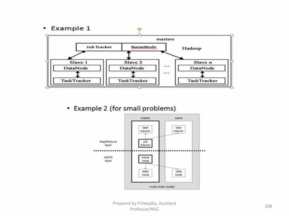
• Hadoop cluster has a Master/Slave Architecture

• Typically one machine in the cluster is designated as

the NameNode and another machine as the JobTracker, exclusively.

- These are the masters.

• The rest of the machines in the cluster act as

both DataNode and TaskTracker. – These are the slaves. Prepared by P.Deepika, Assistant

Professor,PASC103

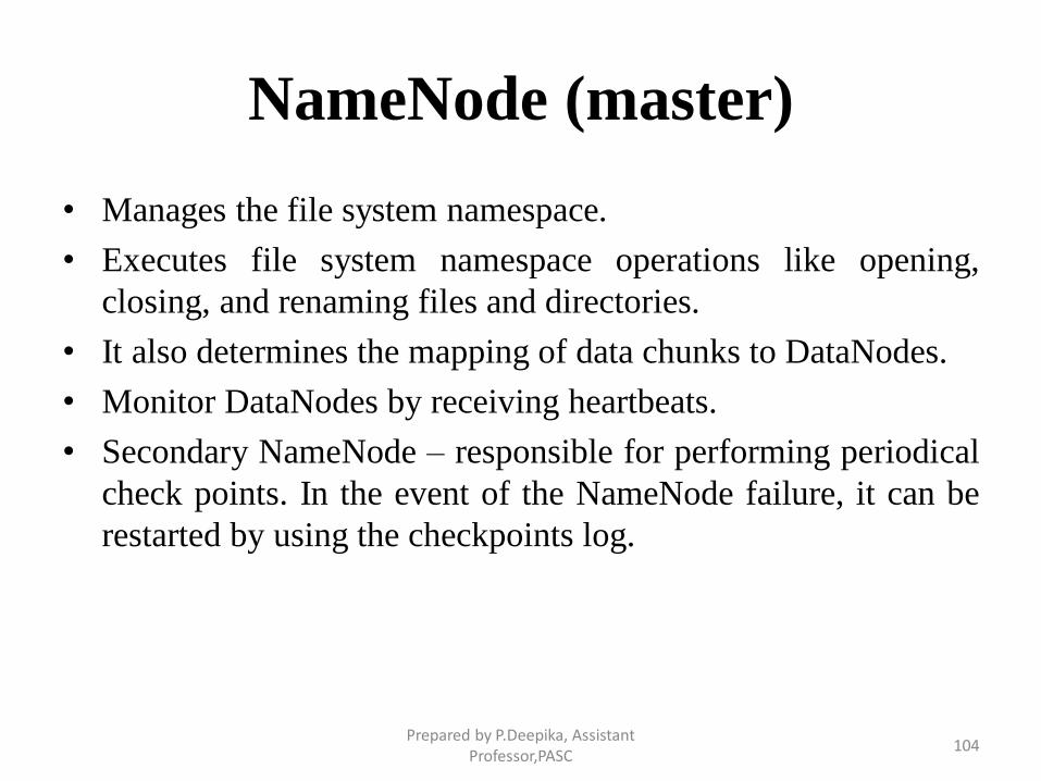
NameNode (master)

• Manages the file system namespace.

• Executes file system namespace operations like opening,

closing, and renaming files and directories.

• It also determines the mapping of data chunks to DataNodes.

• Monitor DataNodes by receiving heartbeats.

• Secondary NameNode – responsible for performing periodical

check points. In the event of the NameNode failure, it can be

restarted by using the checkpoints log.


104

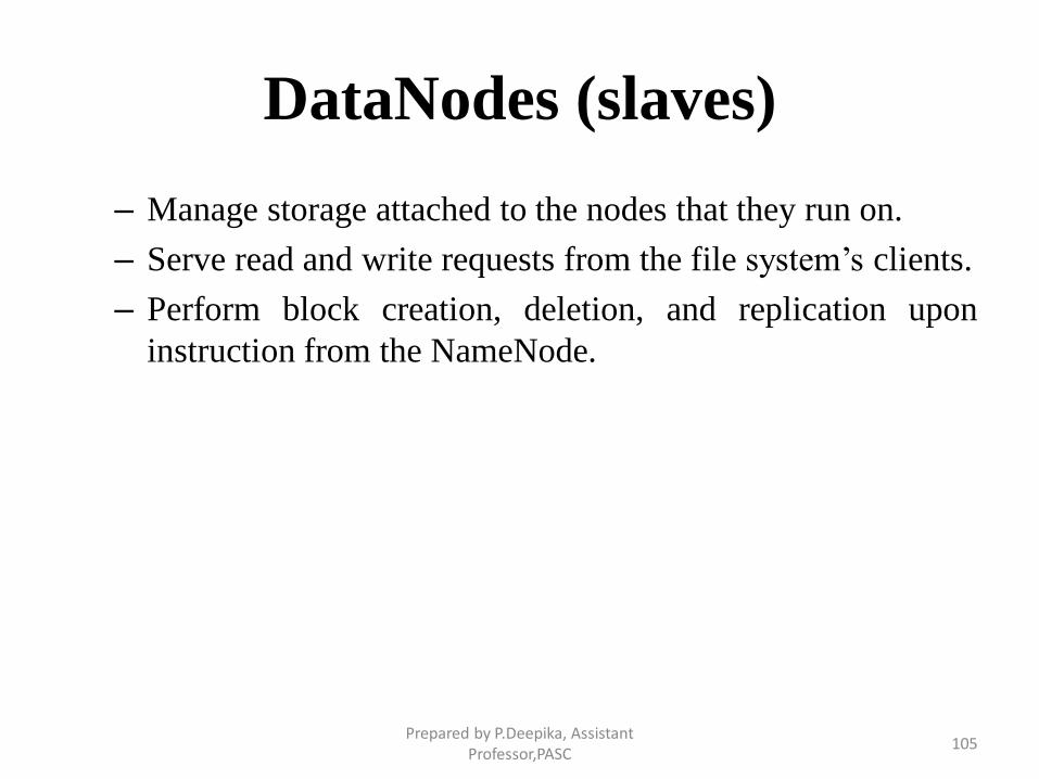
DataNodes (slaves)

– Manage storage attached to the nodes that they run on.

– Serve read and write requests from the file system’s clients.

– Perform block creation, deletion, and replication upon

instruction from the NameNode.


105

JobTracker (master)

– Receive jobs from client

– Talks to the NameNode to determine the location of the

data

– Manage and schedule the entire job

– Split and assign tasks to slaves (TaskTrackers).

– Monitor the slave nodes by receiving heartbeats


106

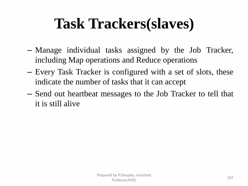
Task Trackers(slaves)

– Manage individual tasks assigned by the Job Tracker,

including Map operations and Reduce operations

– Every Task Tracker is configured with a set of slots, these

indicate the number of tasks that it can accept

– Send out heartbeat messages to the Job Tracker to tell that

it is still alive


107


108

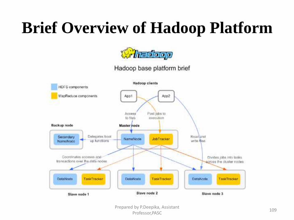
Brief Overview of Hadoop Platform


109

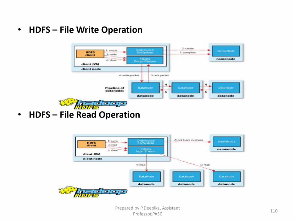
• HDFS – File Write Operation

• HDFS – File Read Operation


110

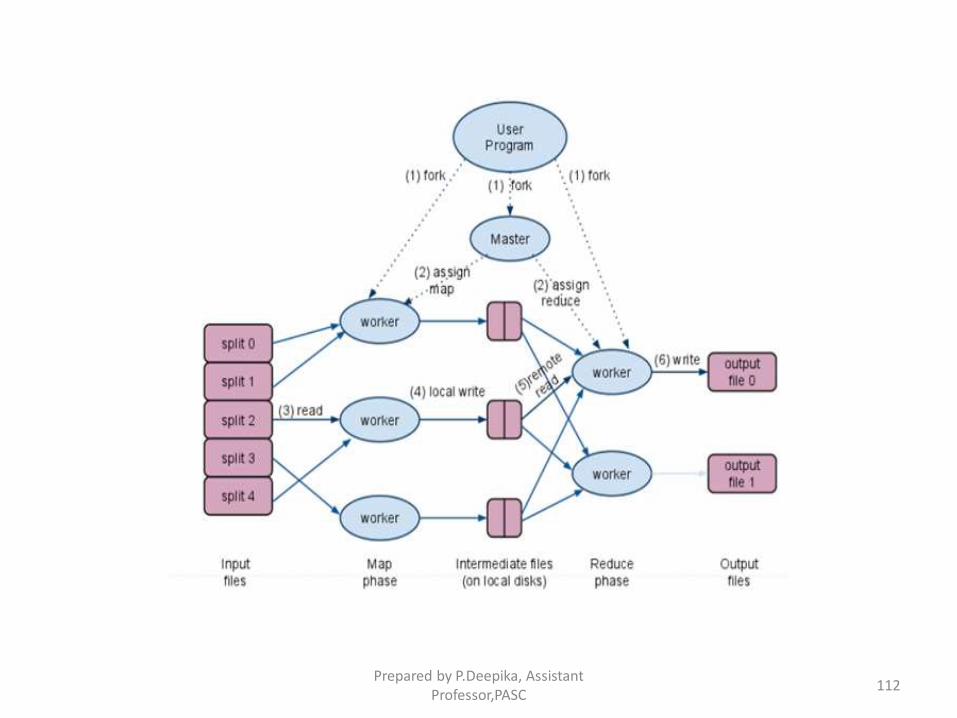
Map Reduce Programming Model

• A programming model developed at Google for large-scale

distributed data processing

• A functional style programming based on ‘Map/Reduce’

functions that are naturally parallelizable across a large cluster

of workstations or PCS.

• Consists of two developer created phases – (i) Map (ii)Reduce

In between ‘Map’ and ‘Reduce’, there is a process of

‘Shuffle’ and ‘Sort’

• “ Reduce” Phase

• Aggregate the intermediate outputs from the ‘Map’ process

and reduces the set of intermediate values associated with the

same key.Prepared by P.Deepika, Assistant

Professor,PASC111


112

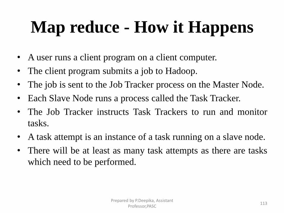
Map reduce - How it Happens

• A user runs a client program on a client computer.

• The client program submits a job to Hadoop.

• The job is sent to the Job Tracker process on the Master Node.

• Each Slave Node runs a process called the Task Tracker.

• The Job Tracker instructs Task Trackers to run and monitor

tasks.

• A task attempt is an instance of a task running on a slave node.

• There will be at least as many task attempts as there are tasks

which need to be performed.


113

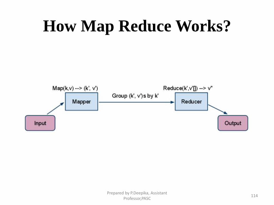
How Map Reduce Works?


114

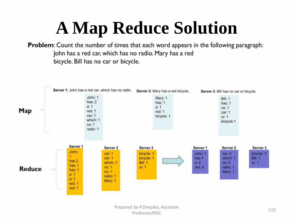
A Map Reduce Solution


115

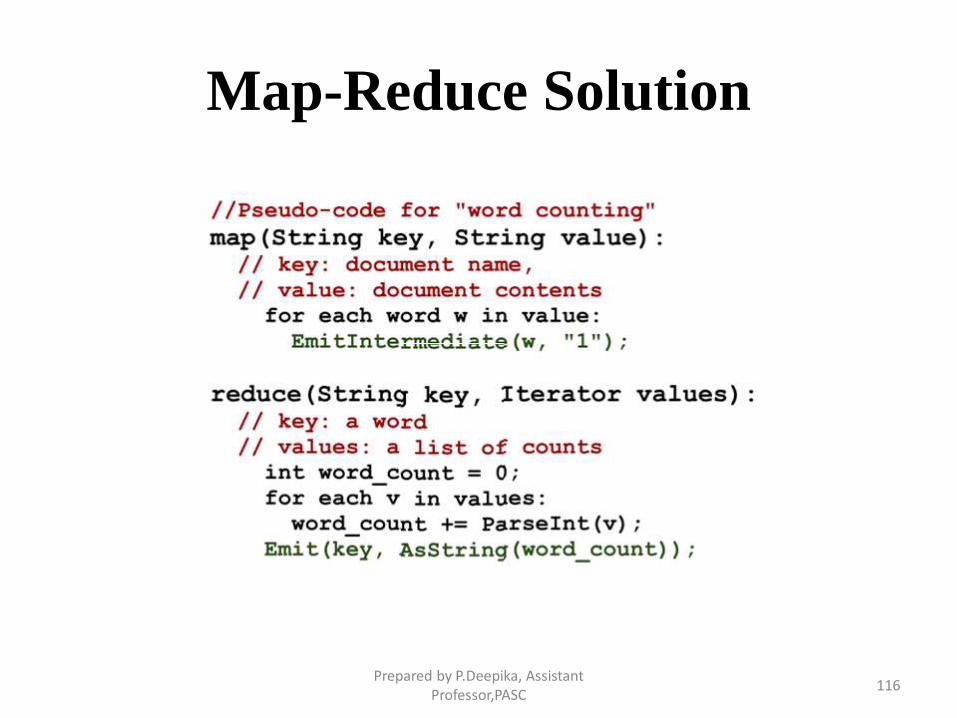
Map-Reduce Solution


116

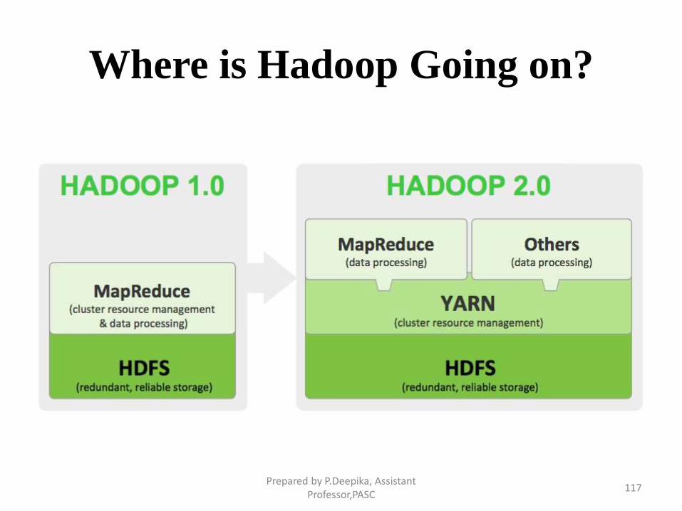
Where is Hadoop Going on?


117

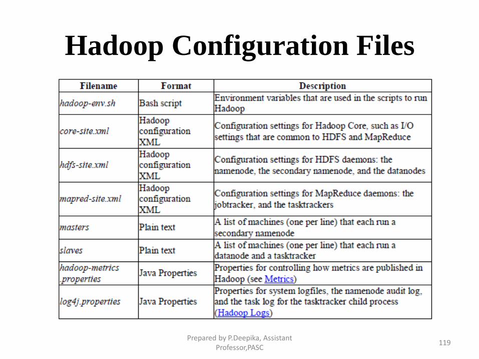
Hadoop Configuration

• There are handful of files for controlling the configuration of a

Hadoop installation; the most important ones are ….

– hadoop-env.sh

– core-site.xml

– hdfs-site.xml

– mapred-site.xml

– masters

– slaves

– hadoop-metrics .properties

– log4j.properties

– These files are all found in the conf directory of the

• Hadoop distributionPrepared by P.Deepika, Assistant

Professor,PASC118

Hadoop Configuration Files


119

Environment Setting - hadoop-

env.sh.• HADOOP_HEAPSIZE property – used to set the memory for each daemons (By

default 1 GB)

• mapred.tasktracker.map.tasks.maximum- The maximum number of map tasks that

can run on a tasktracker at one time (By defaults 2 tasks)

• mapred.tasktracker.reduce.tasks.maximum – The maximum number of reduce asks

that can run on a tasktracker at one time (By defaults 2 tasks)

• The location of the Java implementation to use is determined by the JAVA_HOME

setting.

• HADOOP_SECONDARYNAMENODE_OPTS – to increase the secondary

namenode memory

• System logfiles produced by Hadoop are stored in $HADOOP_INSTALL/logs by

default. This can be changed using the HADOOP_LOG_DIR setting

• export HADOOP_LOG_DIR=/var/log/hadoop

• StrictHostKeyChecking - which can be set to “no” to automatically add new host

keys to the known hosts files. The default, “ask” , prompts the user to confirm that

he has verified the key fingerprint, which is not a suitable setting in a large cluster

environmentPrepared by P.Deepika, Assistant

Professor,PASC120

Configuration Management

• Hadoop does not have a single, global location for configuration information

• Each Hadoop node in the cluster has its own set of configuration files, and it is up

to administrators to ensure that they are kept in sync across the system

• Hadoop is designed so that it is possible to have a single set of configuration files

that are used for all master and worker machines

• Control scripts

• Hadoop comes with scripts for running commands and starting and stopping

daemons across the whole cluster.

• Scripts can be found in the bin directory . To use these scripts, developer has to say

the Hadoop which machines are in the cluster

• There are two files for this purpose, called masters and slaves, each of which

contains a list of the machine hostnames or IP addresses one per line

• masters file - which machine or machines should run a secondary namenode

• The slaves file lists the machines that the datanodes and tasktrackers should run on.


121

Hadoop Eco-system

• Hadoop has become the kernel of the distributed operating

system for Big Data

• No one uses the kernel alone

• There’s a large library of programs that complement the base

Hadoop framework and give companies the specific tools they

need to get the desired Hadoop results.

• A collection of projects at Apache – called Hadoop Eco-

System Tools


122

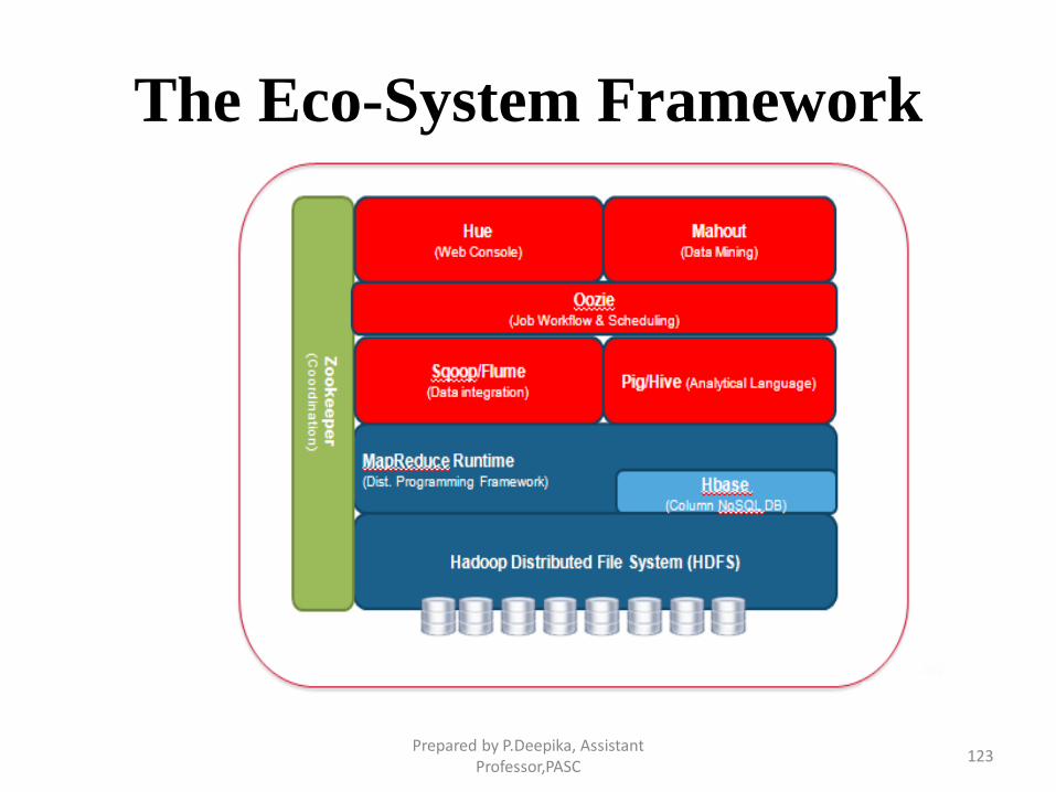
The Eco-System Framework


123

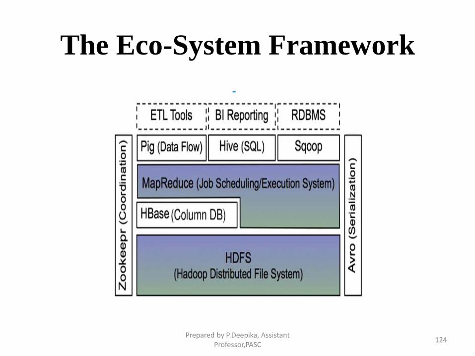
The Eco-System Framework


124

Pig / Hive – Analytical Language

• Although Map Reduce is very powerful, it can also be

complex to master

• Many organizations have business or data analysts who are

skilled at writing SQL queries, but not at writing Java code

• Many organizations have programmers who are skilled at

writing code in scripting languages

• Hive and Pig are two projects which evolved separately to help

such people analyze huge amounts of data via Map Reduce

– Hive was initially developed at Facebook, Pig at Yahoo!


125

Hive• What is Hive?

– An SQL-like interface to Hadoop

• Hive is not a relational database, but a query engine that supports the parts of SQL

specific to querying data, with some additional support for writing new tables or files.

• Data Warehouse infrastructure that provides data summarization and ad hoc querying on

top of Hadoop

– MapRuduce for execution

– HDFS for storage

• Hive is a SQL-based data warehouse system for Hadoop that facilitates data

summarization, ad hoc queries, and the analysis of large datasets stored in Hadoop-

compatible file systems (e.g., HDFS, MapR-FS, and S3) and some NoSQL databases.

• Hive’s SQL dialect is called HiveQL. Queries are translated to MapReduce jobs to

exploit the scalability of MapReduce.

• Hive QL

– Basic-SQL : Select, From, Join, Group-By

– Equi-Join, Muti-Table Insert, Multi-Group-By

• Batch query


126

Pig

• A high-level scripting language (Pig Latin)

• Pig Latin, the programming language for Pig provides common data

manipulation operations, such as grouping, joining, and filtering.

• Pig generates Hadoop MapReduce jobs to perform the data flows.

• This high-level language for ad-hoc analysis allows developers to inspect

HDFS stored data without the need to learn the complexities of the

MapReduce framework, thus simplifying the access to the data.

• The Pig Latin scripting language is not only a higher-level data flow

language

• It has operators similar to SQL (e.g., FILTER and JOIN) that are translated

into a series of map and reduce functions.

• Pig Latin, in essence, is designed to fill the gap between the declarative

style of SQL and the low-level procedural style of MapReduce.


127

When Pig & Hive

• Hive is a good choice

– When you want to query the data

– When you need an answer for specific questions

– If you are familiar with SQL

• Pig is a good choice

– For ETL (Extract Transform- Load)

– For preparing data for easier analysis

– When you have long series of steps to perform


128

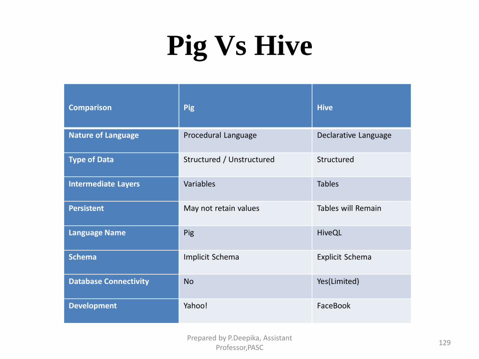
Pig Vs Hive

Comparison Pig Hive

Nature of Language Procedural Language Declarative Language

Type of Data Structured / Unstructured Structured

Intermediate Layers Variables Tables

Persistent May not retain values Tables will Remain

Language Name Pig HiveQL

Schema Implicit Schema Explicit Schema

Database Connectivity No Yes(Limited)

Development Yahoo! FaceBook


129

• Mahout

Machine-learning tool

Distributed and scalable machine learning algorithms on the

Hadoop platform

Building intelligent applications easier and faster

• Mahout Use-cases

Yahoo: Spam Detection

Adobe: User Targeting

Amazon: Personalization Platform


130

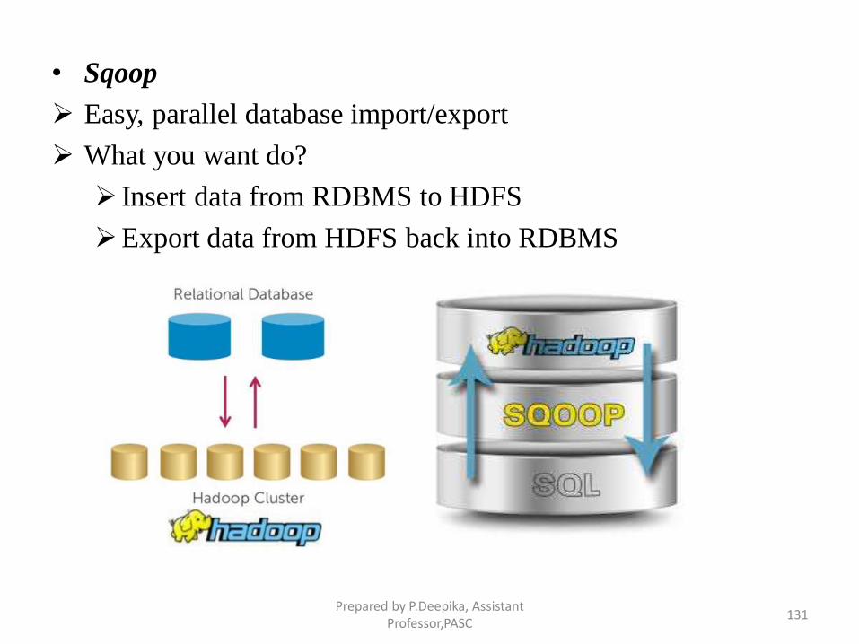
• Sqoop

Easy, parallel database import/export

What you want do?

Insert data from RDBMS to HDFS

Export data from HDFS back into RDBMS


131

HBase• HBase is a column-oriented database management system that runs on top

of HDFS

• Unlike relational database systems, HBase does not support a structured

query language like SQL;

• HBase isn’t a relational data store at all. Hbase applications are written in

Java much like a typical Map Reduce application.

• A centralized service for maintaining

– Configuration information

– Providing distributed synchronization

• A set of tools to build distributed applications that can safely handle partial

failures

• Zoo Keeper was designed to store coordination data

– Status information

– Configuration

– Location information


132

Flume• A distributed data collection service

• It efficiently collecting, aggregating, and moving large amounts of data

• Fault tolerant, many failover and recovery mechanism

• One-stop solution for data collection of all formats

– OOZIE

• A Java web application

• Oozie is a workflow scheduler for Hadoop

• Component independent with

– MapReduce

– Hive

– Pig

– Sqoop

• Triggered

– Time

– DataPrepared by P.Deepika, Assistant

Professor,PASC133

Tools used in Big Data

• Where processing is hosted?

Distributed Servers / Cloud (e.g. Amazon EC2)

• Where data is stored?

Distributed Storage (e.g. Amazon S3)

• What is the programming model?

Distributed Processing (e.g. MapReduce)

• How data is stored & indexed?

High-performance schema-free databases (e.g. MongoDB)

• What operations are performed on data?

Analytic / Semantic Processing


134

UNIT IV


135

Map Reduce Algorithm

• Map Reduce is a framework using which we can write

applications to process huge amounts of data, in parallel, on

large clusters of commodity hardware in a reliable manner.

• The Map Reduce algorithm contains two important tasks,

namely Map and Reduce.

• Secondly, reduce task, which takes the output from a map as

an input and combines those data tuples into a smaller set of

tuples. As the sequence of the name Map Reduce implies, the

reduce task is always performed after the map job.


136

Mapper

• Map takes a set of data and converts it into another set of data,

where individual elements are broken down into tuples key/value

pairs.

Record Reader: Converts a byte-oriented view of the input.

Map: It works on the key-value pairs produced by Record Reader

and generates zero or more intermediate key-value pairs.

Combiner: It is an optional function and it is also called as local

reducer. It takes intermediate key-value pairs and applies user

specific aggregate function to corresponding mapper.

Partitioner: It takes the intermediate key-value pairs produced by

the mapper and splits them into shard, and sends the shard to the

particular reducer.


137

Reducer

• It reduces a set of intermediate values to a smaller set of values. It

has 3 primary phases.

Shuffle and Sort: It takes the output of all the partitioners and

downloads them into the local machine where the reducer is

running. Then these individual data pipes are sorted by the key

which produces larger data sets. This sort groups similar words so

that their values can be easily iterated over by the reduce task.

Reduce: It takes the grouped data, applies reduce function, and

processes one group at a time. It produces various operations such

as aggregation, filtering and combining data. Once it is done the

output is sent to the output format.

Output Format: It separates key-value pairs with tab and writes it

out to a file using record writer.


138

Combiner

• It is an optimization technique for Map Reduce Job.

• The reducer class is said to be the combiner class.

• The difference between combiner and reducer classes is as follows.

• Output generated by combiner is intermediate data and it is passed

to the reducer.

• Output of the reducer is passed to the output file on disk.

• Map Reduce supports searching, Sorting and also Compression.

PARTITIONER:

• The partitioning happens after map phase and before reduce phase.

• The number of partitioners are equal to the number of reducers


139

What is Hive?

• Hive is a data warehouse infrastructure tool to process

structured data in Hadoop.

• It resides on top of Hadoop to summarize Big Data, and makes

querying and analyzing easy.

• Initially Hive was developed by Facebook, later the Apache

Software Foundation took it up and developed it further as an

open source under the name Apache Hive.

• It is used by different companies. For example, Amazon uses it

in Amazon Elastic MapReduce.


140

Features of Hive

• Here are the features of Hive:

It stores schema in a database and processed data into

HDFS.

It is designed for OLAP.

It provides SQL type language for querying called HiveQL

or HQL.

It is familiar, fast, scalable, and extensible.

• Hive is not

A relational database

A design for OnLine Transaction Processing (OLTP)

A language for real-time queries and row-level updates


141

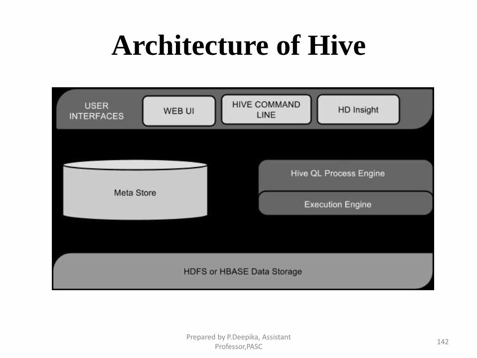
Architecture of Hive


142

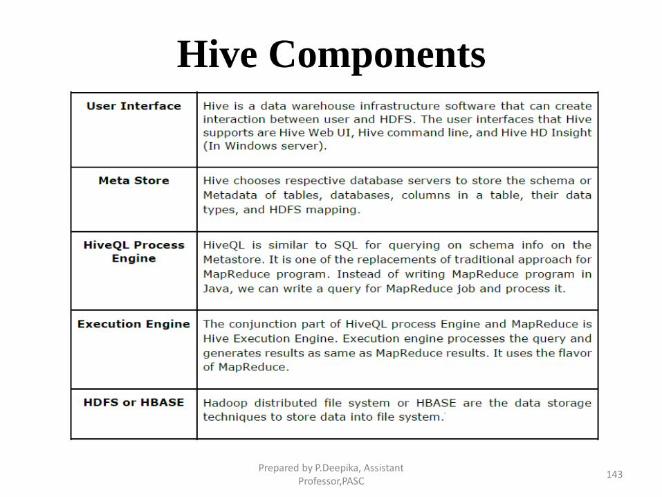
Hive Components


143

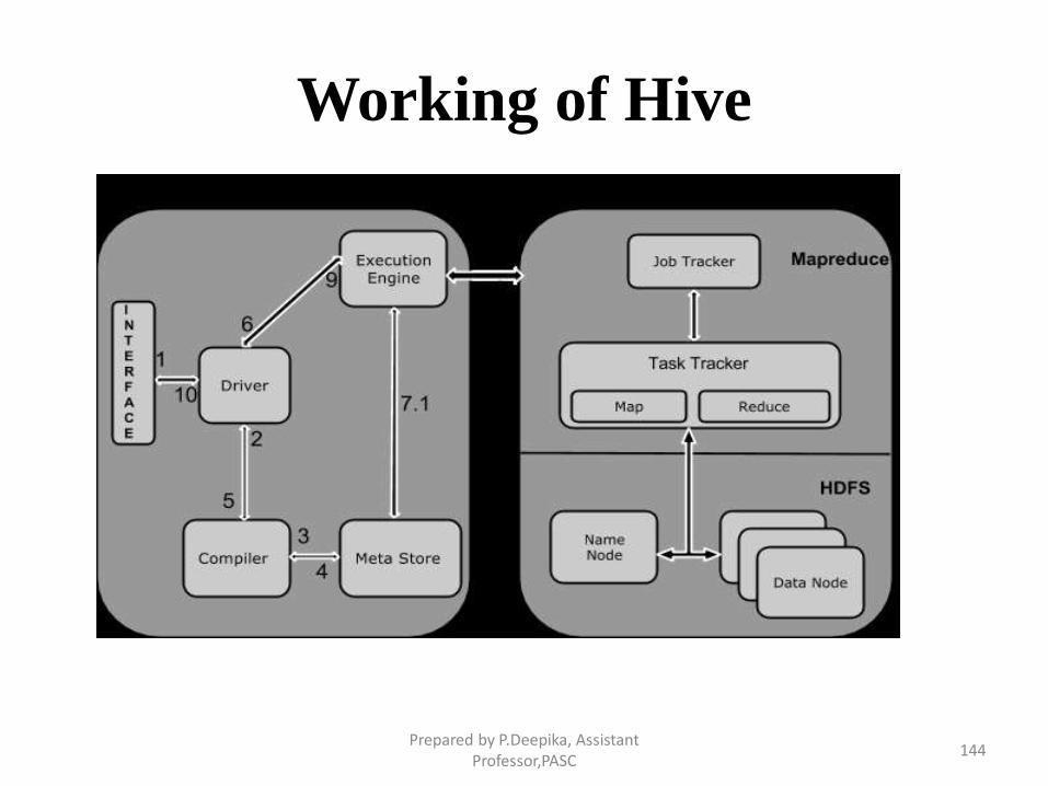
Working of Hive


144

Step Operation

1 Execute Query

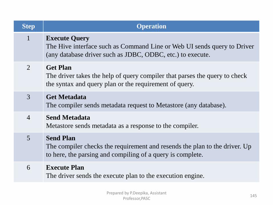
The Hive interface such as Command Line or Web UI sends query to Driver

(any database driver such as JDBC, ODBC, etc.) to execute.

2 Get Plan

The driver takes the help of query compiler that parses the query to check

the syntax and query plan or the requirement of query.

3 Get Metadata

The compiler sends metadata request to Metastore (any database).

4 Send Metadata

Metastore sends metadata as a response to the compiler.

5 Send Plan

The compiler checks the requirement and resends the plan to the driver. Up

to here, the parsing and compiling of a query is complete.

6 Execute Plan

The driver sends the execute plan to the execution engine.


145

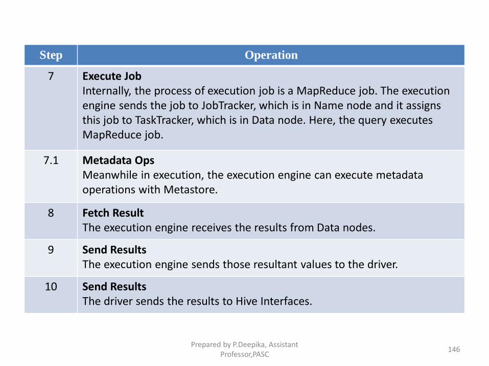
Step Operation

7 Execute Job Internally, the process of execution job is a MapReduce job. The execution engine sends the job to JobTracker, which is in Name node and it assigns this job to TaskTracker, which is in Data node. Here, the query executes MapReduce job.

7.1 Metadata Ops Meanwhile in execution, the execution engine can execute metadata operations with Metastore.

8 Fetch Result The execution engine receives the results from Data nodes.

9 Send Results The execution engine sends those resultant values to the driver.

10 Send Results The driver sends the results to Hive Interfaces.


146

Hive - Data Types

• All the data types in Hive are classified into four types, given

as follows:

Column Types

Literals

Null Values

Complex Types


147

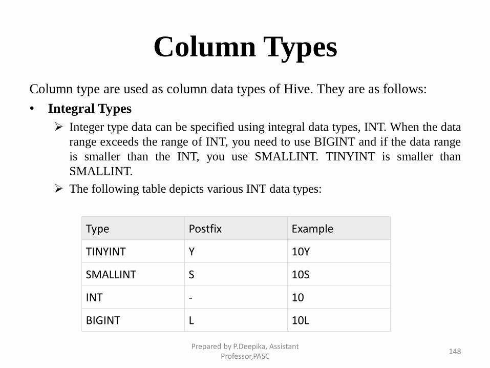
Column Types

Column type are used as column data types of Hive. They are as follows:

• Integral Types

Integer type data can be specified using integral data types, INT. When the data

range exceeds the range of INT, you need to use BIGINT and if the data range

is smaller than the INT, you use SMALLINT. TINYINT is smaller than

SMALLINT.

The following table depicts various INT data types:

Type Postfix Example

TINYINT Y 10Y

SMALLINT S 10S

INT - 10

BIGINT L 10L


148

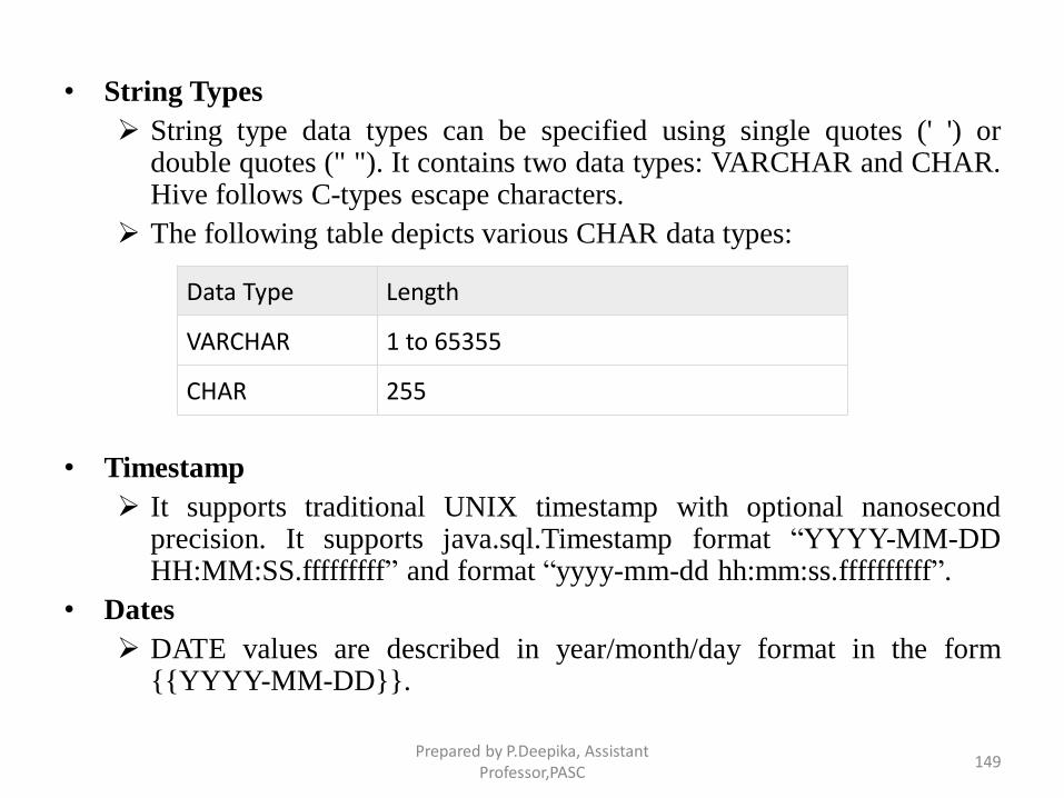
• String Types

String type data types can be specified using single quotes (' ') ordouble quotes (" "). It contains two data types: VARCHAR and CHAR.Hive follows C-types escape characters.

The following table depicts various CHAR data types:

• Timestamp

It supports traditional UNIX timestamp with optional nanosecondprecision. It supports java.sql.Timestamp format “YYYY-MM-DDHH:MM:SS.fffffffff” and format “yyyy-mm-dd hh:mm:ss.ffffffffff”.

• Dates

DATE values are described in year/month/day format in the form{{YYYY-MM-DD}}.

Data Type Length

VARCHAR 1 to 65355

CHAR 255


149

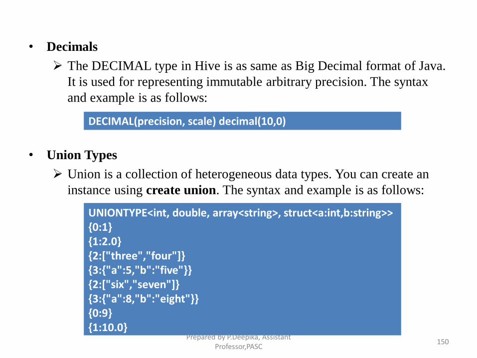
• Decimals

The DECIMAL type in Hive is as same as Big Decimal format of Java.

It is used for representing immutable arbitrary precision. The syntax

and example is as follows:

• Union Types

Union is a collection of heterogeneous data types. You can create an

instance using create union. The syntax and example is as follows:

DECIMAL(precision, scale) decimal(10,0)

UNIONTYPE<int, double, array<string>, struct<a:int,b:string>> {0:1} {1:2.0} {2:["three","four"]} {3:{"a":5,"b":"five"}} {2:["six","seven"]} {3:{"a":8,"b":"eight"}} {0:9} {1:10.0}


150

• Literals

The following literals are used in Hive:

Floating Point Types

Floating point types are nothing but numbers with decimal points.

Generally, this type of data is composed of DOUBLE data type.

Decimal Type

Decimal type data is nothing but floating point value with higher range

than DOUBLE data type. The range of decimal type is approximately -

10-308 to 10308.

Null Value

Missing values are represented by the special value NULL.


151

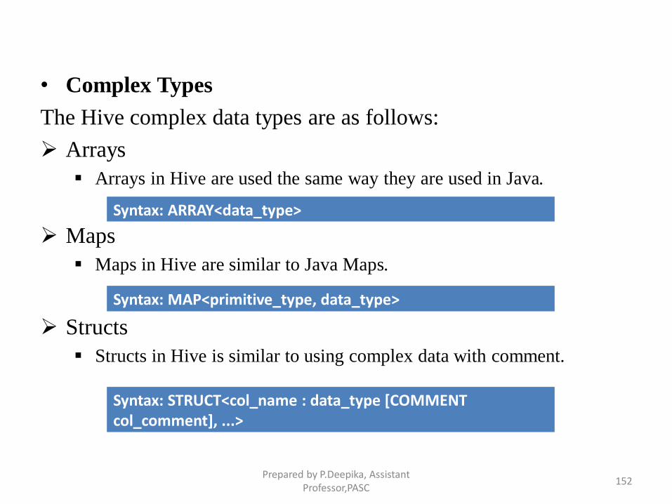
• Complex Types

The Hive complex data types are as follows:

Arrays

Arrays in Hive are used the same way they are used in Java.

Maps

Maps in Hive are similar to Java Maps.

Structs

Structs in Hive is similar to using complex data with comment.

Syntax: ARRAY<data_type>

Syntax: MAP<primitive_type, data_type>

Syntax: STRUCT<col_name : data_type [COMMENT col_comment], ...>


152

Hive File Formats

• Apache Hive supports several familiar file formats used in

Apache Hadoop.

• Hive can load and query different data file created by other

Hadoop components such as Pig or MapReduce.

• Following are the Apache Hive different file formats:

Text File

Sequence File

RC File

AVRO File

ORC File

Parquet File


153

Hive Text File Format

• Hive Text file format is a default storage format. You can use the

text format to interchange the data with other client application.

• Data is stored in lines, with each line being a record. Each lines are

terminated by a newline character (\n).

• The text format is simple plane file format. You can use the

compression (BZIP2) on the text file to reduce the storage spaces.

• Create a TEXT file by add storage option as ‘STORED AS

TEXTFILE’ at the end of a Hive CREATE TABLE command.

Example

Create table textfile_table

(column_specs)

stored as textfile;


154

Hive Sequence File Format

• Sequence files are Hadoop flat files which stores values in binary

key-value pairs.

• The sequence files are in binary format and these files are able to

split. The main advantages of using sequence file is to merge two or

more files into one file.

• Create a sequence file by add storage option as ‘STORED AS

SEQUENCEFILE’ at the end of a Hive CREATE TABLE

command.

Example

Create table sequencefile_table

(column_specs)

stored as sequencefile;


155

Hive RC File Format

• RCFile is row columnar file format. This is another form of Hive file

format which offers high row level compression rates.

• If you have requirement to perform multiple rows at a time then you can

use RCFile format.

• The RCFile are very much similar to the sequence file format. This file

format also stores the data as key-value pairs.

• Create RCFile by specifying ‘STORED AS RCFILE’ option at the end of

a CREATE TABLE Command:

Example

Create table RCfile_table

(column_specs)

stored as rcfile;


156

Hive AVRO File Format

• AVRO is open source project that provides data serialization and

data exchange services for Hadoop. You can exchange data between

Hadoop ecosystem and program written in any programming

languages. Avro is one of the popular file format in Big Data

Hadoop based applications.

• Create AVRO file by specifying ‘STORED AS AVRO’ option at the

end of a CREATE TABLE Command.

Example

Create table avro_table

(column_specs)

stored as avro;


157

Hive ORC File Format

• The ORC file stands for Optimized Row Columnar file format. TheORC file format provides a highly efficient way to store data inHive table.

• This file system was actually designed to overcome limitations ofthe other Hive file formats. The Use of ORC files improvesperformance when Hive is reading, writing, and processing datafrom large tables.

• Create ORC file by specifying ‘STORED AS ORC’ option at theend of a CREATE TABLE Command.

ExampleCreate table orc_table

(column_specs)

stored as orc;


158

Hive Parquet File Format

• Parquet is a column-oriented binary file format. The parquet

is highly efficient for the types of large-scale queries.

• Parquet is especially good for queries scanning particular

columns within a particular table.

• The Parquet table uses compression Snappy, gzip; currently

Snappy by default.

Example

Create table parquet_table

(column_specs)

stored as parquet;


159

Create Database Statement

• Create Database is a statement used to create a database in

Hive. A database in Hive is a namespace or a collection of

tables.

• The syntax for this statement is as follows:

• Here, IF NOT EXISTS is an optional clause, which notifies

the user that a database with the same name already exists.

CREATE DATABASE|SCHEMA [IF NOT EXISTS] <database name>


160

Create Database Statement

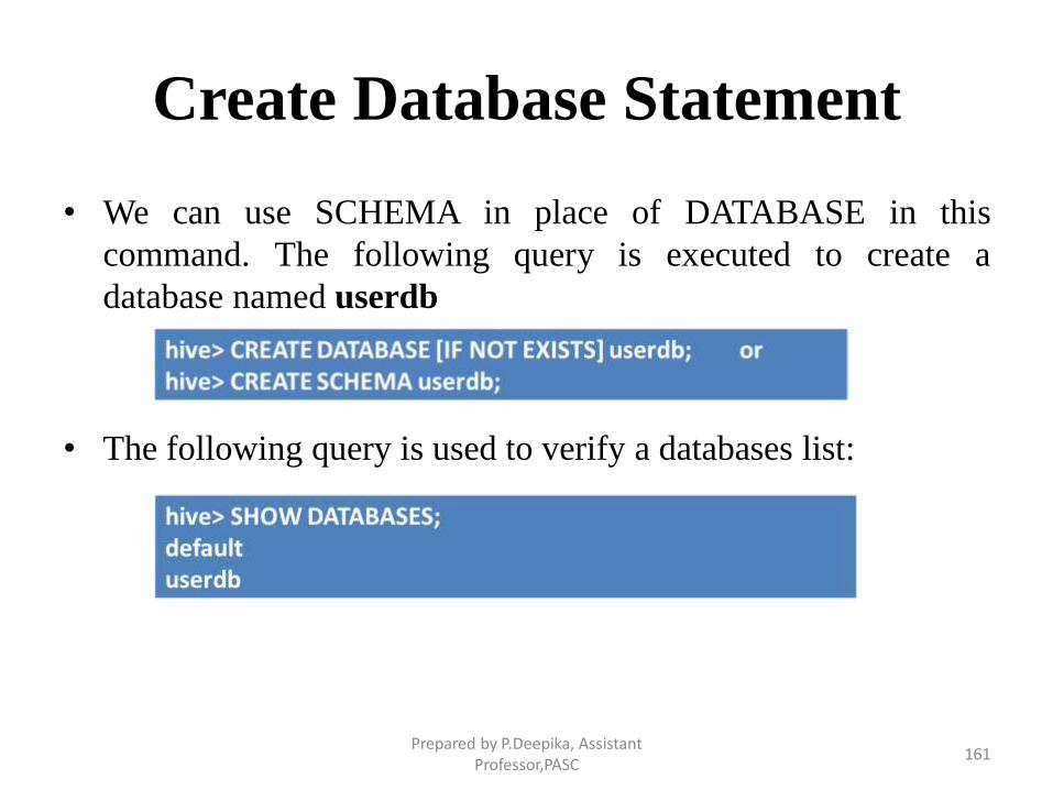
• We can use SCHEMA in place of DATABASE in this

command. The following query is executed to create a

database named userdb

• The following query is used to verify a databases list:


161

Drop Database Statement

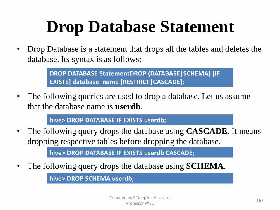
• Drop Database is a statement that drops all the tables and deletes the

database. Its syntax is as follows:

• The following queries are used to drop a database. Let us assume

that the database name is userdb.

• The following query drops the database using CASCADE. It means

dropping respective tables before dropping the database.

• The following query drops the database using SCHEMA.

DROP DATABASE StatementDROP (DATABASE|SCHEMA) [IF EXISTS] database_name [RESTRICT|CASCADE];

hive> DROP DATABASE IF EXISTS userdb;

hive> DROP DATABASE IF EXISTS userdb CASCADE;

hive> DROP SCHEMA userdb;


162

Create Table Statement

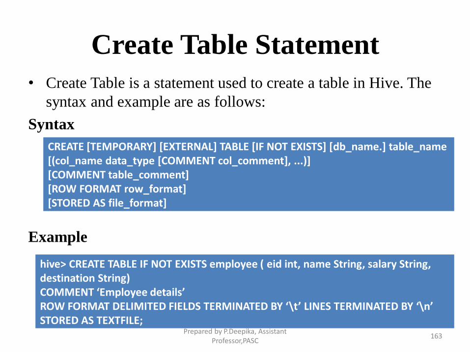
• Create Table is a statement used to create a table in Hive. The

syntax and example are as follows:

Syntax

Example

CREATE [TEMPORARY] [EXTERNAL] TABLE [IF NOT EXISTS] [db_name.] table_name[(col_name data_type [COMMENT col_comment], ...)] [COMMENT table_comment] [ROW FORMAT row_format] [STORED AS file_format]

hive> CREATE TABLE IF NOT EXISTS employee ( eid int, name String, salary String, destination String) COMMENT ‘Employee details’ ROW FORMAT DELIMITED FIELDS TERMINATED BY ‘\t’ LINES TERMINATED BY ‘\n’ STORED AS TEXTFILE;


163

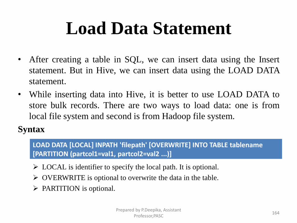
Load Data Statement

• After creating a table in SQL, we can insert data using the Insert

statement. But in Hive, we can insert data using the LOAD DATA

statement.

• While inserting data into Hive, it is better to use LOAD DATA to

store bulk records. There are two ways to load data: one is from

local file system and second is from Hadoop file system.

Syntax

LOCAL is identifier to specify the local path. It is optional.

OVERWRITE is optional to overwrite the data in the table.

PARTITION is optional.

LOAD DATA [LOCAL] INPATH 'filepath' [OVERWRITE] INTO TABLE tablename[PARTITION (partcol1=val1, partcol2=val2 ...)]


164

Load Data Statement

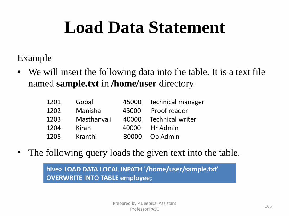
Example

• We will insert the following data into the table. It is a text file

named sample.txt in /home/user directory.

• The following query loads the given text into the table.

1201 Gopal 45000 Technical manager 1202 Manisha 45000 Proof reader 1203 Masthanvali 40000 Technical writer 1204 Kiran 40000 Hr Admin 1205 Kranthi 30000 Op Admin

hive> LOAD DATA LOCAL INPATH '/home/user/sample.txt' OVERWRITE INTO TABLE employee;


165

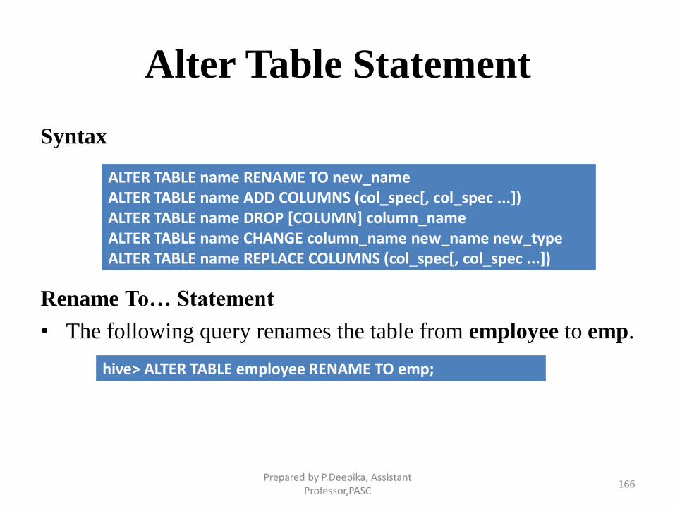
Alter Table Statement

Syntax

Rename To… Statement

• The following query renames the table from employee to emp.

ALTER TABLE name RENAME TO new_nameALTER TABLE name ADD COLUMNS (col_spec[, col_spec ...]) ALTER TABLE name DROP [COLUMN] column_nameALTER TABLE name CHANGE column_name new_name new_typeALTER TABLE name REPLACE COLUMNS (col_spec[, col_spec ...])

hive> ALTER TABLE employee RENAME TO emp;


166

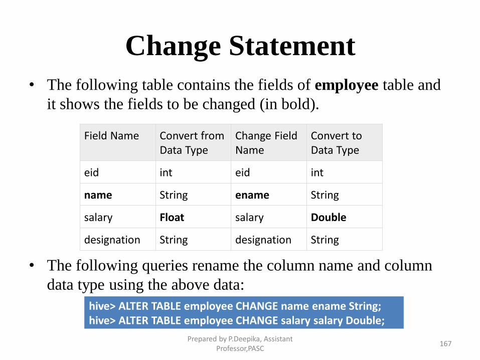
Change Statement

• The following table contains the fields of employee table and

it shows the fields to be changed (in bold).

• The following queries rename the column name and column

data type using the above data:

Field Name Convert from Data Type

Change Field Name

Convert to Data Type

eid int eid int

name String ename String

salary Float salary Double

designation String designation String

hive> ALTER TABLE employee CHANGE name ename String; hive> ALTER TABLE employee CHANGE salary salary Double;


167

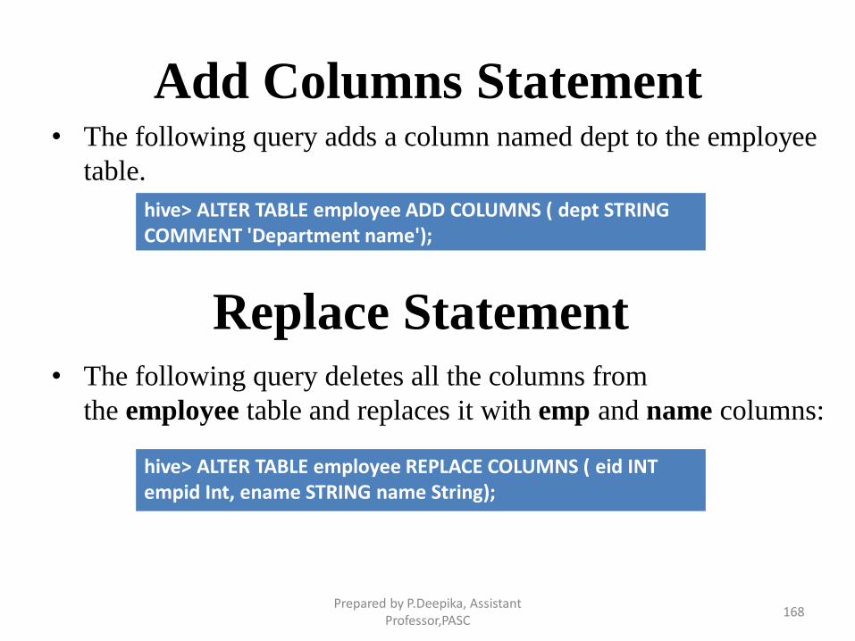
Add Columns Statement• The following query adds a column named dept to the employee

table.

• The following query deletes all the columns from

the employee table and replaces it with emp and name columns:

hive> ALTER TABLE employee ADD COLUMNS ( dept STRING COMMENT 'Department name');

hive> ALTER TABLE employee REPLACE COLUMNS ( eid INT empid Int, ename STRING name String);

Replace Statement


168

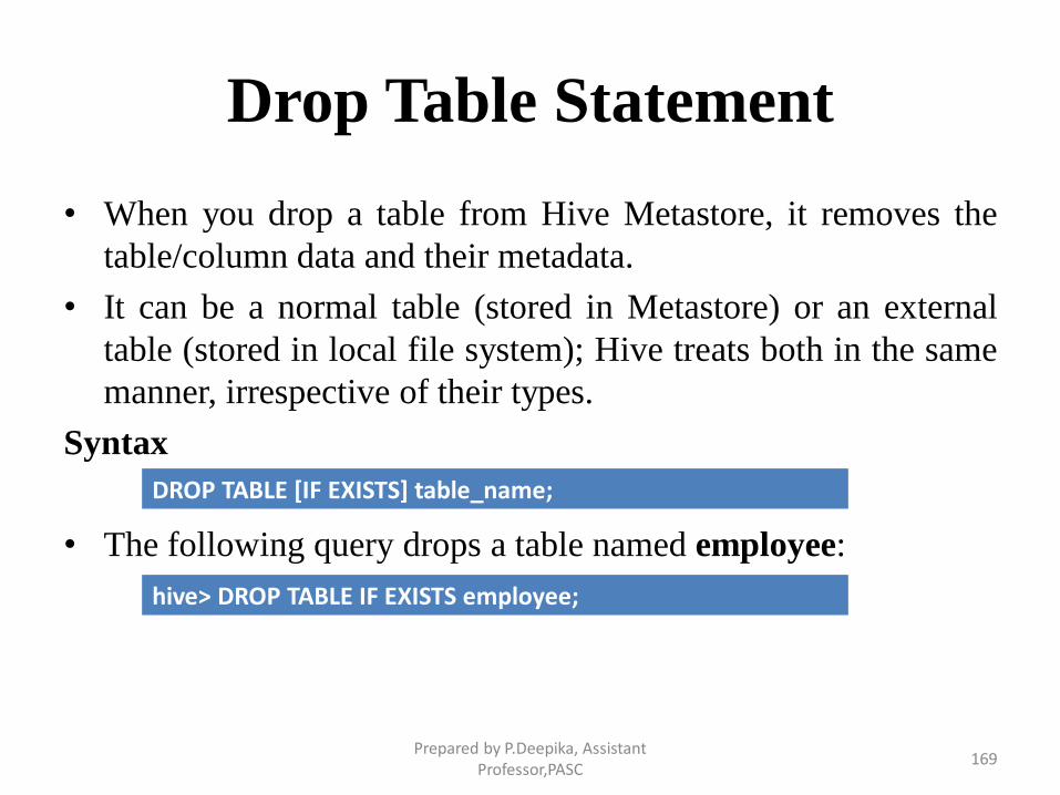
Drop Table Statement

• When you drop a table from Hive Metastore, it removes the

table/column data and their metadata.

• It can be a normal table (stored in Metastore) or an external

table (stored in local file system); Hive treats both in the same

manner, irrespective of their types.

Syntax

• The following query drops a table named employee:

DROP TABLE [IF EXISTS] table_name;

hive> DROP TABLE IF EXISTS employee;


169

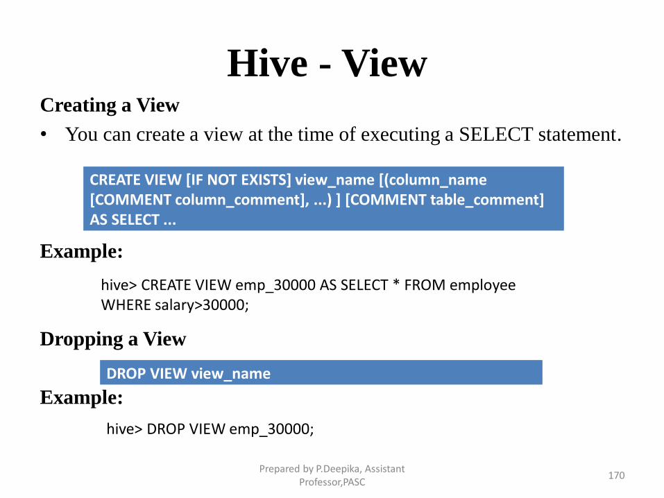
Hive - ViewCreating a View

• You can create a view at the time of executing a SELECT statement.

Example:

Dropping a View

Example:

CREATE VIEW [IF NOT EXISTS] view_name [(column_name[COMMENT column_comment], ...) ] [COMMENT table_comment] AS SELECT ...

DROP VIEW view_name

hive> CREATE VIEW emp_30000 AS SELECT * FROM employee WHERE salary>30000;

hive> DROP VIEW emp_30000;


170

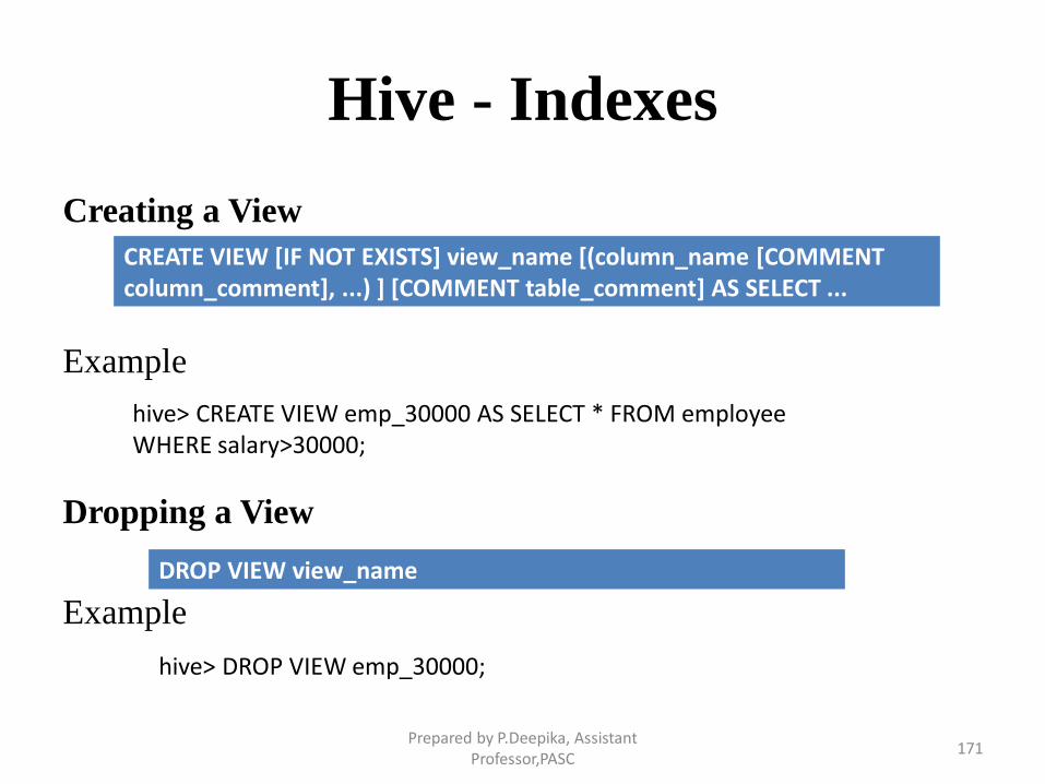
Hive - Indexes

Creating a View

Example

Dropping a View

Example

CREATE VIEW [IF NOT EXISTS] view_name [(column_name [COMMENT column_comment], ...) ] [COMMENT table_comment] AS SELECT ...

hive> CREATE VIEW emp_30000 AS SELECT * FROM employee WHERE salary>30000;

DROP VIEW view_name

hive> DROP VIEW emp_30000;


171

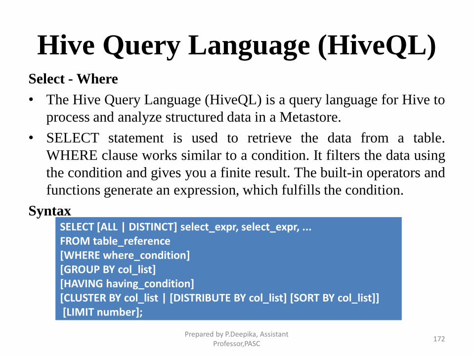
Hive Query Language (HiveQL)Select - Where

• The Hive Query Language (HiveQL) is a query language for Hive to

process and analyze structured data in a Metastore.

• SELECT statement is used to retrieve the data from a table.

WHERE clause works similar to a condition. It filters the data using

the condition and gives you a finite result. The built-in operators and

functions generate an expression, which fulfills the condition.

SyntaxSELECT [ALL | DISTINCT] select_expr, select_expr, ... FROM table_reference[WHERE where_condition] [GROUP BY col_list] [HAVING having_condition] [CLUSTER BY col_list | [DISTRIBUTE BY col_list] [SORT BY col_list]][LIMIT number];


172

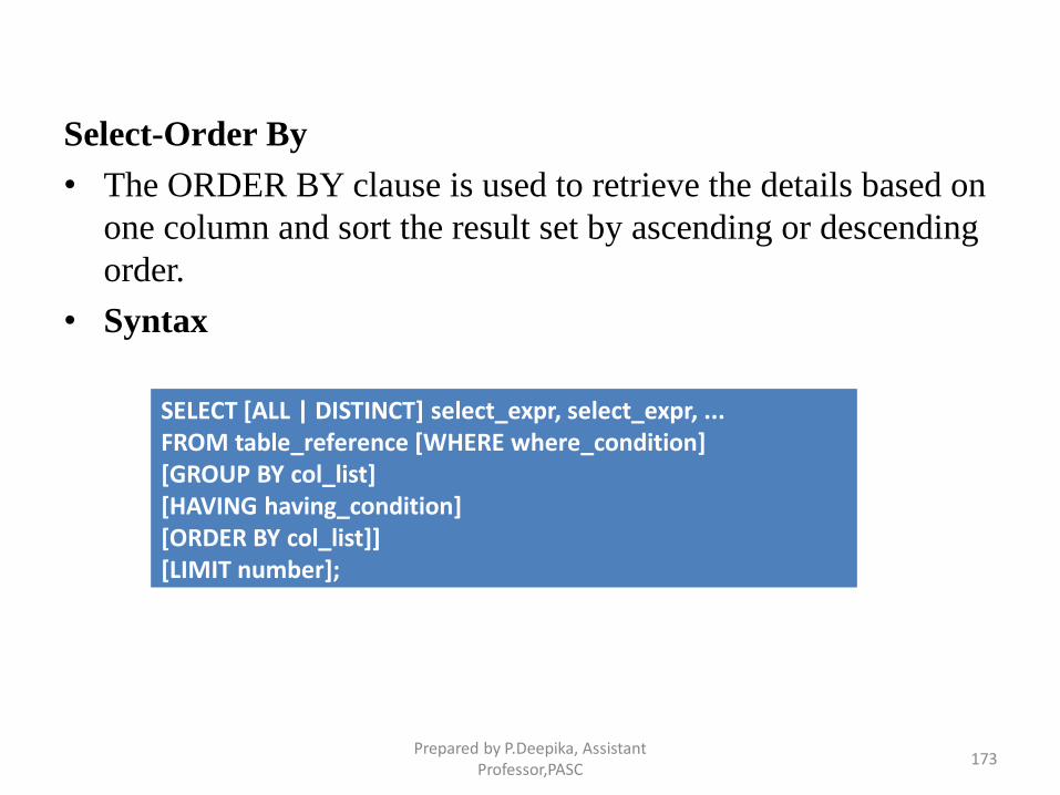
Select-Order By

• The ORDER BY clause is used to retrieve the details based on

one column and sort the result set by ascending or descending

order.

• Syntax

SELECT [ALL | DISTINCT] select_expr, select_expr, ... FROM table_reference [WHERE where_condition] [GROUP BY col_list] [HAVING having_condition] [ORDER BY col_list]] [LIMIT number];


173

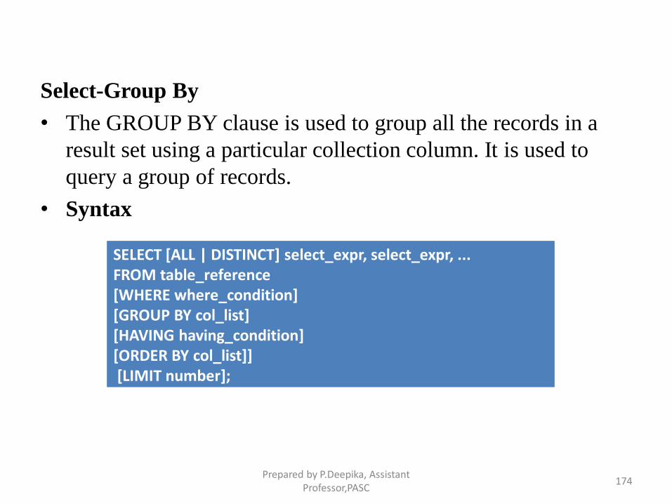
Select-Group By

• The GROUP BY clause is used to group all the records in a

result set using a particular collection column. It is used to

query a group of records.

• Syntax

SELECT [ALL | DISTINCT] select_expr, select_expr, ... FROM table_reference[WHERE where_condition] [GROUP BY col_list] [HAVING having_condition] [ORDER BY col_list]][LIMIT number];


174

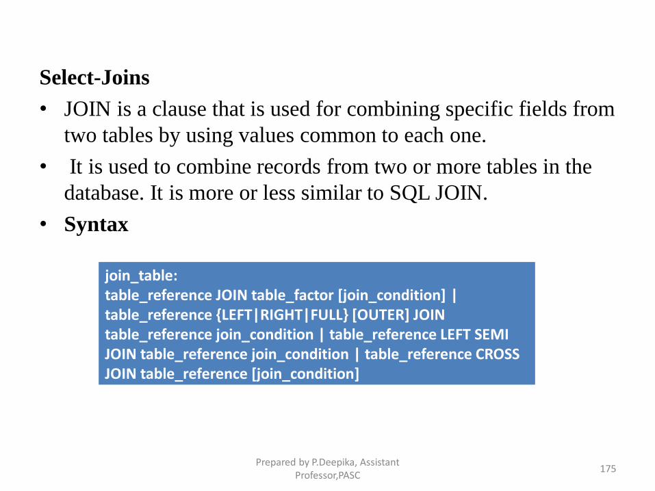
Select-Joins

• JOIN is a clause that is used for combining specific fields from

two tables by using values common to each one.

• It is used to combine records from two or more tables in the

database. It is more or less similar to SQL JOIN.

• Syntax

join_table: table_reference JOIN table_factor [join_condition] | table_reference {LEFT|RIGHT|FULL} [OUTER] JOIN table_reference join_condition | table_reference LEFT SEMI JOIN table_reference join_condition | table_reference CROSS JOIN table_reference [join_condition]


175

• RC File Implementation:

RC File(Record Columnar File) is a data placement structure

that determines how to store relational tables on computer

clusters.

• SERDE:

SerDe stands for Serializer/Deserializer

Contains the logic to convert unstructured data into records.

Implemented using Java.

Serializers are used at the time of writing.

Deserializers are used at query time.

• User Defined Function (UDF):

In Hive, custom functions are defined by UDF.


176

UNIT V


177

Machine Learning

• In learning algorithms, we utilize sample data, feed it to

system and then train the system to produce appropriate

model.

• For example, for email classification, we can compile

thousands of example messages for spam and we can then

make the system to learn to distinguish between a mail that

qualifies as a spam message and the email that is not spam.

• In this situation we may not able to identify the process

completely , but we can construct an appropriate model.

• This helps us to create patterns, which can then be used to

understand the process or to make predictions. This is known

as Machine learning.Prepared by P.Deepika, Assistant

Professor,PASC178

• Example:

Google Search Engine

Facebook

• Definition:

A computer program is said to learn from experience E

with respect to some task T and some performance P, if its

performance on T, as measured by P, improves with

experience E.

• Machine learning algorithms:

Supervised

Unsupervised


179

Linear Regression

• It is used to estimate real values (cost of houses, number of

calls, total sales etc.) based on continuous variable(s). Here,

we establish relationship between independent and dependent

variables by fitting a best line. This best fit line is known as

regression line and represented by a linear equation Y= a *X +

b.

• In this equation:

• Y – Dependent Variable

• a – Slope

• X – Independent variable

• b – Intercept


180

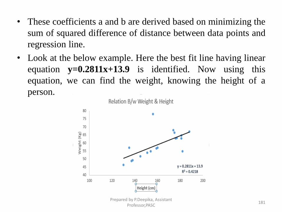
• These coefficients a and b are derived based on minimizing the

sum of squared difference of distance between data points and

regression line.

• Look at the below example. Here the best fit line having linear

equation y=0.2811x+13.9 is identified. Now using this

equation, we can find the weight, knowing the height of a

person.


181

https://www.analyticsvidhya.com/wp-content/uploads/2015/08/Linear_Regression.png

https://www.analyticsvidhya.com/wp-content/uploads/2015/08/Linear_Regression.png

• Linear Regression is of mainly two types:

Simple Linear Regression

Multiple Linear Regression.

• Simple Linear Regression is characterized by one independent

variable.

• And, Multiple Linear Regression(as the name suggests) is

characterized by multiple (more than 1) independent

variables.

• While finding best fit line, you can fit a polynomial or

curvilinear regression.

• And these are known as polynomial or curvilinear regression.


182

R Code

#Load Train and Test datasets

#Identify feature and response variable(s) and values must be numeric and nu

mpy arrays

x_train <- input_variables_values_training_datasets

y_train <- target_variables_values_training_datasets

x_test <- input_variables_values_test_datasets

x <- cbind(x_train,y_train)

# Train the model using the training sets and check score

linear <- lm(y_train ~ ., data = x)

summary(linear)

#Predict Output

predicted= predict(linear,x_test)


183

Clustering

• Clustering is the process of grouping similar objects together.

• It is an example of unsupervised learning.

• Clustering can be used to group items in a supermarket.

• Clustering algorithms are mainly used for natural groupings.

Categories:

• Hierarchical: It identifies the cluster within a cluster. For

example, inside sports news article there could be news on

baseball, basket ball etc.

• Partitional: It creates a fixed number of clusters. K-means

clustering algorithm belongs to this category.


184

K-Means Clustering Algorithm

• It is a type of unsupervised algorithm which solves the

clustering problem. Its procedure follows a simple and

easy way to classify a given data set through a certain number

of clusters (assume k clusters). Data points inside a cluster are

homogeneous and heterogeneous to peer groups.


185

https://www.analyticsvidhya.com/wp-content/uploads/2015/08/splatter_ink_blot_texture_by_maki_tak-d5p6zph.jpg

https://www.analyticsvidhya.com/wp-content/uploads/2015/08/splatter_ink_blot_texture_by_maki_tak-d5p6zph.jpg

How K-means forms cluster

• K-means picks k number of points for each cluster known as

centroids.

• Each data point forms a cluster with the closest centroids i.e. k

clusters.

• Finds the centroid of each cluster based on existing cluster

members. Here we have new centroids.

• As we have new centroids, repeat step 2 and 3. Find the closest

distance for each data point from new centroids and get

associated with new k-clusters. Repeat this process until

convergence occurs i.e. centroids does not change.


186

How to determine value of K

• In K-means, we have clusters and each cluster has its own

centroid. Sum of square of difference between centroid and the

data points within a cluster constitutes within sum of square

value for that cluster. Also, when the sum of square values for

all the clusters are added, it becomes total within sum of

square value for the cluster solution.

• We know that as the number of cluster increases, this value

keeps on decreasing but if you plot the result you may see that

the sum of squared distance decreases sharply up to some

value of k, and then much more slowly after that. Here, we can

find the optimum number of cluster.


187

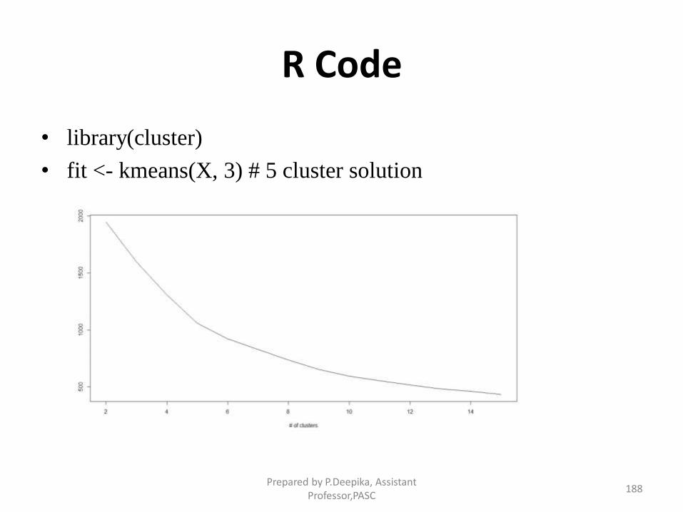
R Code

• library(cluster)

• fit <- kmeans(X, 3) # 5 cluster solution


188

https://www.analyticsvidhya.com/wp-content/uploads/2015/08/Kmenas.png

https://www.analyticsvidhya.com/wp-content/uploads/2015/08/Kmenas.png

kNN (k- Nearest Neighbours)

• It can be used for both classification and regression problems.

However, it is more widely used in classification problems in

the industry.

• K nearest neighbours is a simple algorithm that stores all

available cases and classifies new cases by a majority vote of

its k neighbours.

• The case being assigned to the class is most common amongst

its K nearest neighbours measured by a distance function.

• These distance functions can be Euclidean, Manhattan,

Minkowski and Hamming distance.


189

• First three functions are used for continuous function and

fourth one (Hamming) for categorical variables.

• If K = 1, then the case is simply assigned to the class of its

nearest neighbour.

• At times, choosing K turns out to be a challenge while

performing kNN modelling.

• Things to consider before selecting kNN:

• KNN is computationally expensive

• Variables should be normalized else higher range variables can

bias it


190

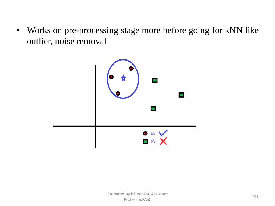
• Works on pre-processing stage more before going for kNN like

outlier, noise removal


191

https://www.analyticsvidhya.com/wp-content/uploads/2015/08/KNN.png

https://www.analyticsvidhya.com/wp-content/uploads/2015/08/KNN.png

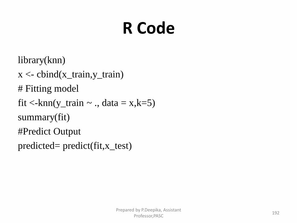
R Code

library(knn)

x <- cbind(x_train,y_train)

# Fitting model

fit <-knn(y_train ~ ., data = x,k=5)

summary(fit)

#Predict Output

predicted= predict(fit,x_test)


192

Collaborative Filtering

• It is a technique used for recommendation.

• Let us assume there are two people A & B. A likes Apples and

B also likes Apples.

• In this case we assume that B has similar liking as A.

• So we can go ahead and recommend options for A & B as

well.

• It is a category of information filtering. It is predicting the user

preferences based on the preferences of a group of users.

• It can be defined as Social Navigation.


193

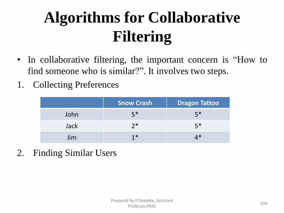
Algorithms for Collaborative

Filtering

• In collaborative filtering, the important concern is “How to

find someone who is similar?”. It involves two steps.

1. Collecting Preferences

2. Finding Similar Users

Snow Crash Dragon Tattoo

John 5* 5*

Jack 2* 5*

Jim 1* 4*


194

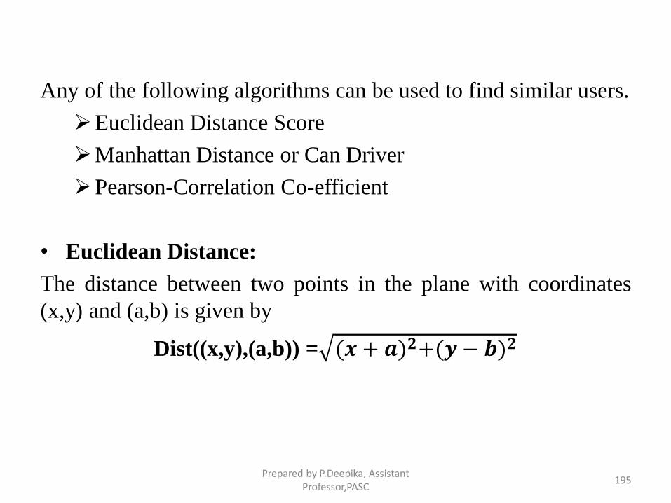
Any of the following algorithms can be used to find similar users.

Euclidean Distance Score

Manhattan Distance or Can Driver

Pearson-Correlation Co-efficient

• Euclidean Distance:

The distance between two points in the plane with coordinates

(x,y) and (a,b) is given by

Dist((x,y),(a,b)) = (𝒙 + 𝒂)𝟐+(𝒚 − 𝒃)𝟐


195

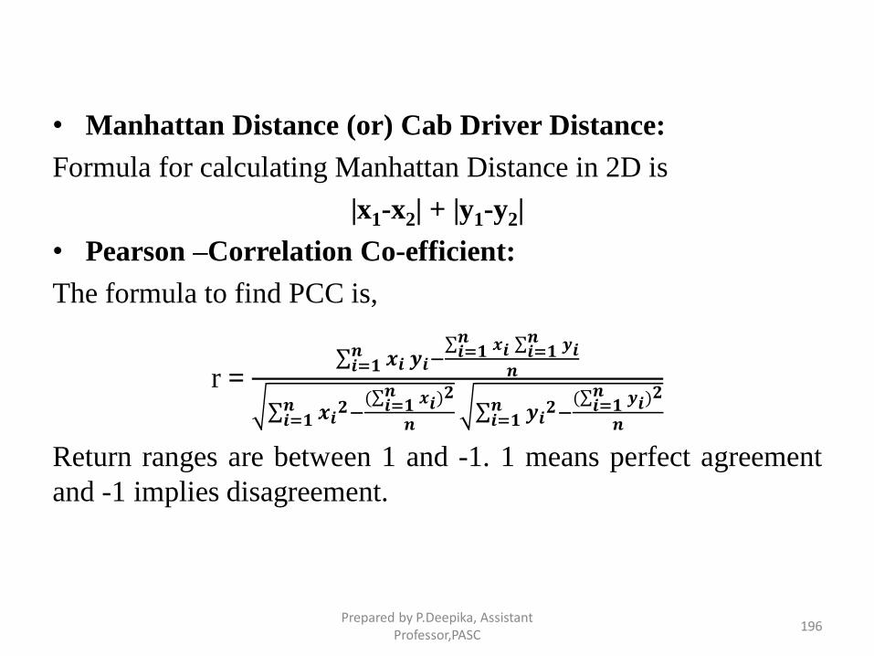
• Manhattan Distance (or) Cab Driver Distance:

Formula for calculating Manhattan Distance in 2D is

|x1-x2| + |y1-y2|

• Pearson –Correlation Co-efficient:

The formula to find PCC is,

r = σ𝒊=𝟏𝒏 𝒙𝒊 𝒚𝒊−

σ𝒊=𝟏𝒏 𝒙𝒊 σ𝒊=𝟏

𝒏 𝒚𝒊𝒏

σ𝒊=𝟏𝒏 𝒙𝒊

𝟐−(σ𝒊=𝟏𝒏 𝒙𝒊)

𝟐

𝒏σ𝒊=𝟏𝒏 𝒚𝒊

𝟐−(σ𝒊=𝟏𝒏 𝒚𝒊)

𝟐

𝒏

Return ranges are between 1 and -1. 1 means perfect agreement

and -1 implies disagreement.


196

Association Rule Mining

• Association rule mining is a procedure which is meant to find

frequent patterns, correlations, associations, or causal

structures from data sets found in various kinds of databases

such as relational databases, transactional databases, and other

forms of data repositories.

• Given a set of transactions, association rule mining aims to

find the rules which enable us to predict the occurrence of a

specific item based on the occurrences of the other items in the

transaction


197

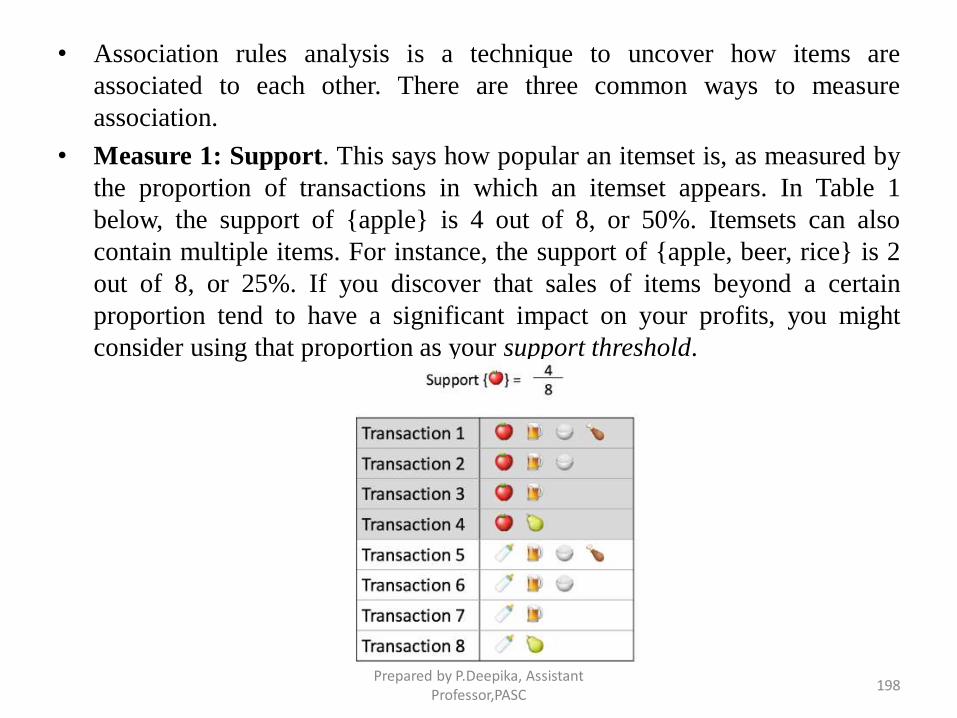
• Association rules analysis is a technique to uncover how items are

associated to each other. There are three common ways to measure

association.

• Measure 1: Support. This says how popular an itemset is, as measured by

the proportion of transactions in which an itemset appears. In Table 1

below, the support of {apple} is 4 out of 8, or 50%. Itemsets can also

contain multiple items. For instance, the support of {apple, beer, rice} is 2

out of 8, or 25%. If you discover that sales of items beyond a certain

proportion tend to have a significant impact on your profits, you might

consider using that proportion as your support threshold.


198

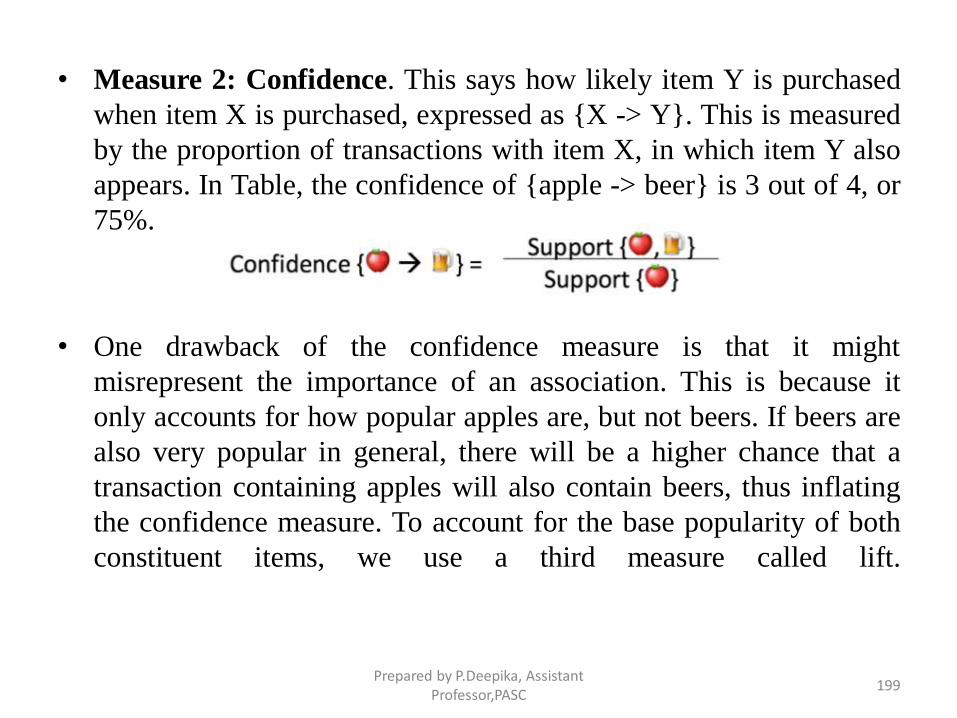
• Measure 2: Confidence. This says how likely item Y is purchased

when item X is purchased, expressed as {X -> Y}. This is measured

by the proportion of transactions with item X, in which item Y also

appears. In Table, the confidence of {apple -> beer} is 3 out of 4, or

75%.

• One drawback of the confidence measure is that it might

misrepresent the importance of an association. This is because it

only accounts for how popular apples are, but not beers. If beers are

also very popular in general, there will be a higher chance that a

transaction containing apples will also contain beers, thus inflating

the confidence measure. To account for the base popularity of both

constituent items, we use a third measure called lift.


199

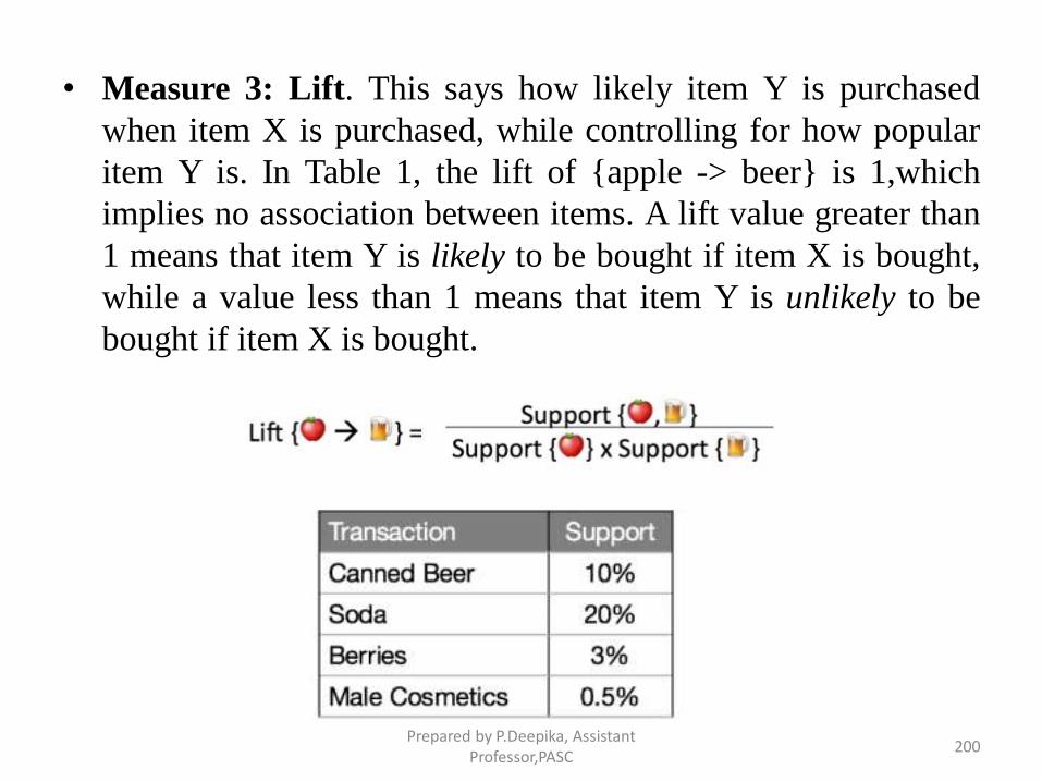
• Measure 3: Lift. This says how likely item Y is purchased

when item X is purchased, while controlling for how popular

item Y is. In Table 1, the lift of {apple -> beer} is 1,which

implies no association between items. A lift value greater than

1 means that item Y is likely to be bought if item X is bought,

while a value less than 1 means that item Y is unlikely to be

bought if item X is bought.


200

Decision Tree

• It is a type of supervised learning algorithm that is mostly used

for classification problems.

• It works for both categorical and continuous

dependent variables.

• In this algorithm, the population is spitted into two or more

homogeneous sets.

• This is done based on most significant attributes/ independent

variables to make as distinct groups as possible.


201

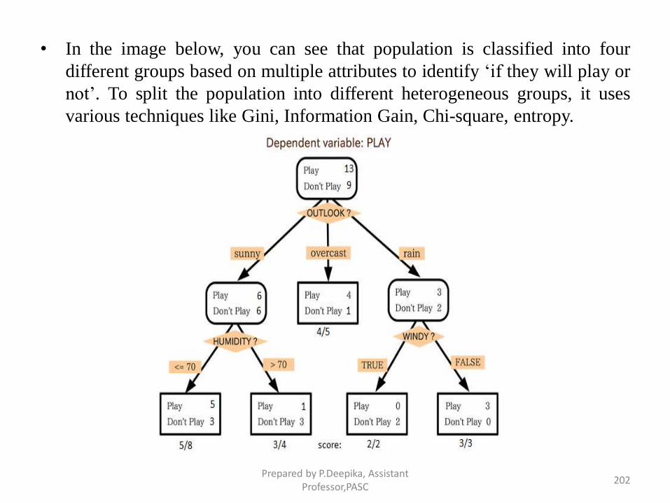
• In the image below, you can see that population is classified into four

different groups based on multiple attributes to identify ‘if they will play or

not’. To split the population into different heterogeneous groups, it uses

various techniques like Gini, Information Gain, Chi-square, entropy.


202

https://www.analyticsvidhya.com/wp-content/uploads/2015/08/IkBzK.png

https://www.analyticsvidhya.com/wp-content/uploads/2015/08/IkBzK.png

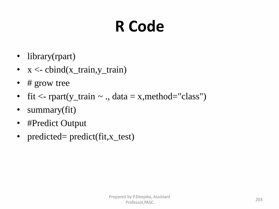
R Code

• library(rpart)

• x <- cbind(x_train,y_train)

• # grow tree

• fit <- rpart(y_train ~ ., data = x,method="class")

• summary(fit)

• #Predict Output

• predicted= predict(fit,x_test)


203

Thank You


204