1

Prepared by:

Anna Watkins

Submitted to:

Dr. Huidae Cho

GISC 3200K

Programming for Geospatial Science & Technology

December 3, 2020

2

Introduction:

Using Python for ArcGIS Pro is a great way to look at area change. A Python toolbox is a great

way to view, create, and edit data. ArcGIS Pro is a wonderful way to map land cover change. According

to Applied Geography, Using current data layers, such as urban boundaries and building footprints,

along with past aerial photographs of the city and census data, a detailed reconstruction of the city of

Pocatello, Idaho was possible for 1941 for both urban form and population. (Jared Ogle, Donna

Delparte, Hannah Sanger 2017)

Urbanization is a complex, multi-dimensional phenomenon that encompasses demographic

dynamics, socio-economic growth, and associated land-cover/use changes (Seto et al.,

2000, Montgomery, 2008, Li et al., 2012, Jiang et al., 2013) Land use and land cover are constantly

changing everyday on local and global scale. The rapid expansion of city worldwide in general has

worsened the predicament of landscape fragmentation in urban greening, especially for some

developing countries (Wanghe, Global Ecology and Conservation) Remote sensing is a great way to study

and observe these changes of the land cover. Land cover is a way to describe physical and biological

cover over a surface that includes the land, water, vegetation, bare soil, and artificial structures.

Common usage of the term “landscape metrics” refers exclusively to indices developed for categorical

map patterns. Landscape metrics are algorithms that quantify specific spatial characteristics of

landscape patches, classes of patches, or entire landscape mosaics (Smith et al., 2009). Land Use and

Land Cover maps are created using remote sensing, there are many different ways of collecting data

using remote sensing and a wide range classification techniques. One of the unique ways of collecting

remote sensing data is by using Landsat 8. Landsat 8 is a satellite that has recent satellite that has been

launched to gather data using Operational Land Imager (OLI) and Thermal Infrared Sensor (TIRS).

The amount of Land use and Land cover change in hall county seems to increase everyday. A

new neighborhood or warehouse seems to be appearing on every street. So how can we find out just

how much Hall county has changed in the last five years? Adding in a Python toolbox or running a script

could help us visualize how much land in Hall county has changed. A Python toolbox is a tool in ArcGIS

Pro that help you take advantage of geoprocessing tools. Chen Zhang says, experimental results suggest

that the proposed software can significantly reduce the workload for modelers who conduct geospatial

agricultural and environmental modeling. (Chen Zang, Liping Di, Zhengwei Yang, Li Lin, Pengyu Hao;

Environmental Modelling & Software 2020) According to SoftwareX, Spatial Design Network Analysis

(sDNA) is a toolbox for 3-d spatial network analysis, especially street/path/urban network analysis,

motivated by a need to use network links as the principal unit of analysis in order to analyse existing

network data. sDNA is usable from QGIS & ArcGIS geographic information systems, AutoCAD, the

command line, and via its own Python API.(Crispin H.V. Cooper) sDNA helps compute mean distances

and closeness.

Forests play a large role in regulating climate, please help reduce levels of carbon dioxide and

greenhouse gases in the atmosphere provider Angel other medical services like biodiversity and

3

watershed protection.( Martin Jung; Ecological Informatics) Deforestation in urban sprawl have changed

the landscape around the globe Deforestation is one of the biggest drives climate change. Urban growth

drives deforestation in two ways the first is people move from rural areas move to the cities for work or

a new lifestyle using up more resources. Second, large meat companies buy land and clear it out for

livestock. Cities have been growing around the globe by about 1.4 million new inhabitant every week.

Urban land area is expanding twice as fast as urban populations urbanization may cause the loss above 2

seven point 4 million acres of prime agricultural land each year.

Study Area:

My study area is Hall County which is located in North East Georgia. Hall County has approximately 429 sq. mi where 37 sq. mi is water from Lake Sidney Lanier. More than half of the Hall County is located in the Upper Oconee River sub-basin of the Altamaha River basin while the other half of Hall County is located in the Upper Chattahoochee River sub-basin of the Apalachicola-Chattahoochee-Flint River Basin. Hall county is heavily forested area with both deciduous and coniferous trees. As of 2010’s census for Hall County, there were 179,684 people, 60,691 households, and 45,275 families residing in Hall. The population density was 457.5 inhabitants per square mile.

Python and satellite imagery:

Satellite imagery is collected everyday across the globe. Global coverage of hrigh resolution imagery of the earth is easily accessible to the public an dis used to help monitor earth and the environment. In the analysis, we will access data from earth explorer, analyze and visualize the data using python. Python is a high-level programming language that has built in data structures that make it very appealing for Rapid Application Development. Python can be easily ran on AcGIS Pro, ArcPy helps to provide ways to preform data analysis, data management, and data conversions on a map. ArcPy allows access to geoprocessing tools and functions. According to Mapping LCLU Using Python Scripting Python, features a dynamic type system and automatic memory management. It supports multiple programming paradigms, including object-oriented, imperative, functional and procedural, and has a large and comprehensive standard library. (Oday Z. Jasim, Khalid I. Hasoon, Noor E. Sadiqe 2019)

In this analysis, Earth Explorer from the USGS website will be used to easily collect all the data. There are a lot of different python packages, however, for this analysis we will be using GDAL. GDAL is a python extension package for programming and manipulating geospatial data. GDAL is easily accessible, when in the Anaconda prompt simply type:

C :\ Users \ annaw>conda ins tall gdal

Along with gdal, numpy will also be used in the analysis. Using numpy and gdal together can be used to read raster data as numerical arrays.

4

Landsat 8:

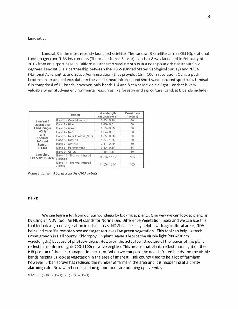
Landsat 8 is the most recently launched satellite. The Landsat 8 satellite carries OLI (Operational Land Imager) and TIRS instruments (Thermal Infrared Sensor). Landsat 8 was launched in February of 2013 from an airport base in California. Landsat 8 satellite orbits in a near-polar orbit at about 98.2 degrees. Landsat 8 is a partnership between the USGS (United States Geological Survey) and NASA (National Aeronautics and Space Administration) that provides 15m-100m resolution. OLI is a push-broom sensor and collects data on the visible, near infrared, and short wave infrared spectrum. Landsat 8 is comprised of 11 bands, however, only bands 1-4 and 8 can sense visible light. Landsat is very valuable when studying environmental resources like forestry and agriculture. Landsat 8 bands include:

Figure 1: Landsat 8 bands from the USGS website

NDVI:

We can learn a lot from our surroundings by looking at plants. One way we can look at plants is by using an NDVI tool. An NDVI stands for Normalized Difference Vegetation Index and we can use this tool to look at green vegetation in urban areas. NDVI is especially helpful with agricultural areas, NDVI helps indicate if a remotely sensed target retrieves live green vegetation. This tool can help us track urban growth in Hall county. Chlorophyll in plant leaves absorbs the visible light (400-700nm wavelengths) because of photosynthesis. However, the actual cell structure of the leaves of the plant reflect near-infrared light( 700-1100nm wavelengths). This means that plants reflect more light on the NIR portion of the electromagnetic spectrum. When we compare the near-infrared bands and the visible bands helping us look at vegetation in the area of interest. Hall county used to be a lot of farmland, however, urban sprawl has reduced the number of farms in the area and it is happening at a pretty alarming rate. New warehouses and neighborhoods are popping up everyday.

NDVI = (NIR - Red) / (NIR + Red)

5

Pycharm:

Pycharm was used to run the script. A 30-day free trial was downloaded onto the computer to

help run the script. In Pycharm, you can run tool, debug and make applications. Pycharm was very easy

to run. Pycharm was great when making the code, it helped creating the script by showing spelling

errors. Pycharm supports Anaconda so it was able to run gdal and numpy with no problem.

Objective:

The goal of the research project is to look at deforestation in around the city of Gainesville,

Georgia located in Hall county. The goal is to use methods of Remote Sensing to be able to get a good

look at what is happening. To conduct our research project we will need to:

1. Collect spatial data

2. Create a ModelBuilder on ArcGis Pro to put all the data together

3. Use Python toolbox to determine how far urban sprawl has taken over Hall County.

Methods and Materials:

Materials:

When looking at urban sprawl, remote sensing is one of the best to get a great visual of what is

happening. But, we can use Python to help look at the big picture. In order to create a Python toolbox to

look at NDVI, important data needs to be collected from the USGS website:

1. 2013 Landsat 8 data

2. 2019 Landsat 8 data

3. 2013 and 2019 NAIP files (2 sets of 6 are need)

Along with our data, to be able to complete an NDVI using Python, a couple of tools need to be added to

the computer to complete our analysis.

1. Anaconda prompt to install:

a. Scikit

6

b. Geopandas

2. Pycharm to help run the script

Extra materials:

1. ArcGis Pro

2. Shapefile of GA counties then clipped to Hall County

Methods:

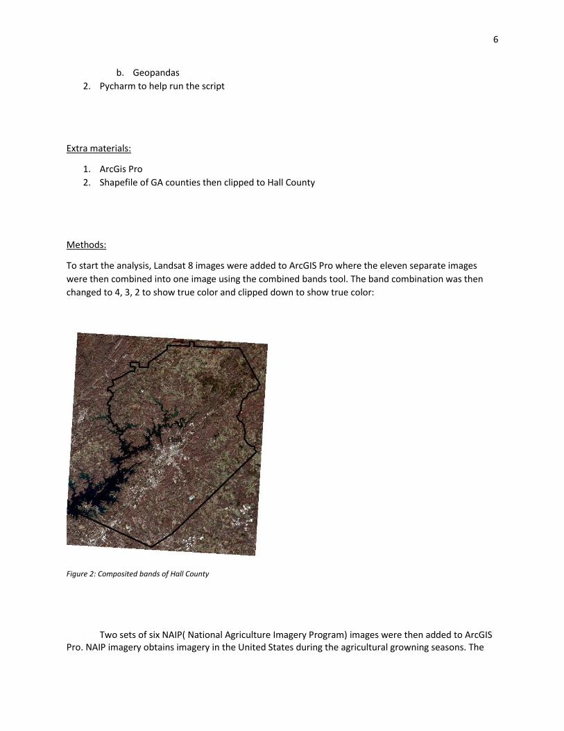
To start the analysis, Landsat 8 images were added to ArcGIS Pro where the eleven separate images

were then combined into one image using the combined bands tool. The band combination was then

changed to 4, 3, 2 to show true color and clipped down to show true color:

Figure 2: Composited bands of Hall County

Two sets of six NAIP( National Agriculture Imagery Program) images were then added to ArcGIS Pro. NAIP imagery obtains imagery in the United States during the agricultural growning seasons. The

7

reason for the NAIP images was to preform an unsupervised classification to model urban sprwl around the city of Gainesville. The NAIP images were converted from mosaic to new raster to produce one single image instead of six separate images. The first NAIP images used were from 2013 and the second set of images were from 2019 to show how the classifications have changed.

Figure 3: Showing unsupervised classification of Gainesville from 2013 and 2019.

For the research project, an unsupervised classification tool was in the works, however, it was

never able to run. For the project, it was important to still show the classification to see the spread of

urban sprawl.

Creating the NDVI toolbox:

The first step when creating the NDVI tool is to add Anaconda prompt to the computer. From

here we can install various python extension packages. We can then start setting up our environment.

The packages that were installed were geopandas and scipy. In the analysis we will be using gdal which

comes in the geopandas extension package.

For our NDVI script, it is important that we extract the visible and near infrared bands. Values

for Landsat 8 are 0-10,000 and the other values need to be filtered out. Because our Landsat data has 11

bands and we only want one output band, we write this portion. So we create a function to write a

8

raster and input a raster dataset. We then want to define a new NDVI function here. We can stack our

operations to get our raster. And lastly, we include our inputs.

Results:

The Python script was ran using Pycharm. It is necessary to switch the 2016 data for the 2019 data and

re-run the script so we have an NDVI for 2016 and an NDVI for 2019. The two scripts will then appear in

the folder that was assigned in the script. The next thing to do is add the scripts to the ArcGIS Project.

Figure 4: 2013 and 2019 NDVI ran by Pycharm

After we have our 2013 and 2019 data, we can run the minus tool. The minus tool is very useful, the

minus tool subtracts the values of the second raster from the first. The equation that will be used is:

OutRas = Minus (InRas1, InRas2)Minus_3d (InRas1, InRas2, OutRas)

The minus tool will show us the difference in the 2013 and 2019 NDVI. The minus tool will help us see

the difference and we can look more into where areas have been deforested. Below is a map of the

minus tool using the 2013 and 2019 data:

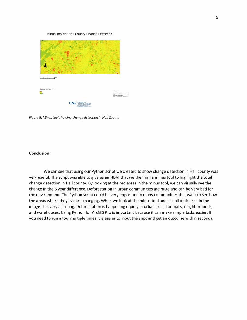
9

Figure 5: Minus tool showing change detection in Hall County

Conclusion:

We can see that using our Python script we created to show change detection in Hall county was

very useful. The script was able to give us an NDVI that we then ran a minus tool to highlight the total

change detection in Hall county. By looking at the red areas in the minus tool, we can visually see the

change in the 6 year difference. Deforestation in urban communities are huge and can be very bad for

the environment. The Python script could be very important in many communities that want to see how

the areas where they live are changing. When we look at the minus tool and see all of the red in the

image, it is very alarming. Deforestation is happening rapidly in urban areas for malls, neighborhoods,

and warehouses. Using Python for ArcGIS Pro is important because it can make simple tasks easier. If

you need to run a tool multiple times it is easier to input the sript and get an outcome within seconds.

10

References:

Jasim, O., Hasoon, K., & Sadiqe, N. (2019). Mapping LCLU Using Python Scripting.

Engineering and Technology Journa. Retrieved from

https://mail.engtechjournal.org/index.php/et/article/view/19/447

Zhang, C., Di, L., Yang, Z., Lin, L., & Hao, P. (2020). Environmental Modelling & Software. A

Toolkit for Agricultural Land Use Modeling of the Conterminous United States Based on

Google Earth Engine. Retrieved 2020, from

https://www.sciencedirect.com/science/article/pii/S1364815219304670

Smith, M. (2019). Environmental Modelling & Software. Geospatial Analysis: A Comprehensive

Guide to Principles, Techniques and Software Tools.

Cooper, C. (2020). SoftwareX. SDNA: 3-d Spatial Network Analysis for GIS, CAD, Command

Line & Python. Retrieved 2020, from

https://www.sciencedirect.com/science/article/pii/S2352711019303401

Jung, M. (2015). Ecological Informantics. Retrieved 2015, from

https://www.sciencedirect.com/science/article/pii/S1574954115001879

Volk, J., & Turner, M. (2019). PRMS-Python: A Python framework for programmatic PRMS

modeling and access to its data structures. Retrieved 2019, from

https://www.sciencedirect.com/science/article/pii/S1364815218308004?via%3Dihub

Work with Landsat Remote Sensing Data in Python. (2020, March 02). Retrieved October 29,

2020, from https://www.earthdatascience.org/courses/use-data-open-source-

python/multispectral-remote-sensing/landsat-in-Python/

Authorship, A., Masnovo, A., Gaelle GourmelonMarketing and Communications

DirectorWorldwatch InstituteJoin VERGE 20: Register here for VERGE 20: October 26-

30, & Gaelle GourmelonMarketing and Communications DirectorWorldwatch Institute.

(n.d.). How urban consumption lies at the root of deforestation. Retrieved October 29,

2020, from https://www.greenbiz.com/article/how-urban-consumption-lies-root-

deforestation

Wanghea, K. (2020). Global Ecology and Conservation. Gravity Model Toolbox: An Automated

and Open-source ArcGIS Tool to Build and Prioritize Ecological Corridors in Urban

11

Landscapes. Retrieved 2020, from

https://www.sciencedirect.com/science/article/pii/S2351989420300433

Hrisko, J. (n.d.). Satellite Imagery Analysis in Python Part III: Land Surface Temperature and

The National Land Cover Database (NLCD).

Python Script:

“9.4 Calculate NDVI Using GDAL.” 9.4 Calculate NDVI Using GDAL | Python Scripting |

Learning Materials, learningzone.rspsoc.org.uk/index.php/Learning-Materials/Python-

Scripting/9.4-Calculate-NDVI-using-GDAL.

Ksund, et al. “Using Python to Calculate NDVI with Multiband Imagery.” Esri Australia

Technical Blog, 14 Feb. 2012, esriaustraliatechblog.wordpress.com/2012/03/14/using-

python-to-calculate-ndvi-with-multiband-imagery/.

“Chapter 2: Your First Remote Sensing Vegetation Index¶.” chapter_2_indices,

ceholden.github.io/open-geo-tutorial/python/chapter_2_indices.html.