Embed Size (px)
Citation preview

ФЕДЕРАЛЬНОЕ АГЕНТСТВО ПО ОБРАЗОВАНИЮ Государственное образовательное учреждение высшего профессионального образования
«ТОМСКИЙ ПОЛИТЕХНИЧЕСКИЙ УНИВЕРСИТЕТ»
V.V. Konev
PREPARATORY COURSE OF MATHEMATICS
Textbook
Рекомендовано в качестве учебного пособия Редакционно-издательским советом
Томского политехнического университета
Издательство Томского политехнического университета
2009
UDС 517 V.V. Konev. Preparatory course of Mathematics. Textbook. The second edition. Tomsk, TPU Press, 2009, 108 pp.
The contents of the book includes three parts: Algebra, Trigonometry and Geometry. Each part contains definitions of main mathematical terms which are explained by making use of different examples.
The textbook can be helpful for English speaking students in order to broaden and methodize their knowledge of mathematics. Reviewed by: V.A. Kilin, Professor of the Higher Mathematics Department, TPU, D.Sc.
1998-2009 © Konev V.V. 1998-2009© Tomsk Polytechnic University
Introduction
The book has been written to help students to broaden and methodize their knowledge of mathematics. First of all, it is designed for students who are studying on their own, but it can be also used by a teacher in the classroom with groups of students. The contents includes three parts: Algebra, Trigonometry and Geometry. Each part contains definitions of main mathematical terms that are explained using a number of different examples. Algebra has the following structure: Chapter 1 begins with a section on the definition of the natural, integer, rational, and real number systems and discusses properties of the basic operations on numbers in these systems. Next, the discussion goes on to properties of absolute values and fraction. Then, intervals and elementary operations on sets are introduced, and operations with radicals and fractional exponents are considered. Chapter 2 includes operations with polynomials and algebraic expressions to provide alternative ways to write the same algebraic expression. It contains many worked examples. Chapter 3 comprises methods of solving linear and quadratic equations and inequalities, providing geometric interpretations of algebraic principles. Chapter 4 includes algebraic, logarithmic, exponential, and other functions and contains finding inverse functions. Graphical properties of a function, such as domain, range, intercepts, and symmetries are also discussed. Chapter 5 describes basic elements of mathematical induction principle, arithmetic and geometric progressions, and the binomial theorem. The concept of mathematical induction is explained using many worked examples that have real significance for practice applications. Geometry covers general topics, such as: • relationships of parts of geometric figures, e.g. medians of triangles, inscribed angles in
circles and so on; • relationships among geometric figures, such as congruence, similarity; • relationships among sets of special quadrilaterals, such as the square, rectangle,
parallelogram, rhombus, and trapezoid; • the properties of triangles, quadrilaterals, polygons, circles, parallel and perpendicular
lines; • the Pythagorean theorem; • computation of perimeters, areas, and volumes of two‐dimensional and three‐
dimensional figures; • the law of sines and the law of cosines. As a rule, the proofs of the theorems are based on using of graphical illustrations. Trigonometry includes: • degree or radian measure of angles; • definition of the trigonometric function; • the trigonometric functions of special angles; • proofs of multiform identities for the trigonometric functions; • graphs of the trigonometric functions; • inverse trigonometric functions and their graphs. Each topic contains graphical illustrations.

Contents
ALGEBRA 1. Real Number System . . . . . . . . . . . . . . . . . . . . . . . . . . . . . . . . . . . . . . . . . . . 7
1.1 Basic Notations and Definitions . . . . . . . . . . . . . . . . . . . . . . . . . . . . . . . 7 1.1.1. Numbers . . . . . . . . . . . . . . . . . . . . . . . . . . . . . . . . . . . . . . . . . . . 7 1.1.2. Properties of Real Numbers . . . . . . . . . . . . . . . . . . . . . . . . . . . . . . . 8
1.2 Absolute Values . . . . . . . . . . . . . . . . . . . . . . . . . . . . . . . . . . . . . . . . . . . 10 1.3 Fractions . . . . . . . . . . . . . . . . . . . . . . . . . . . . . . . . . . . . . . . . . . .. . . . . . . . . . 11 1.4 Sets . . . . . . . . . . . . . . . . . . . . . . . . . . . . . . . . . . . . .. . . . . . . . . . . . . . . . 13
1.4.1 Some Important Sets . . . . . . . . . . . . . . . . . . . . . . . . . . . . . . . 13 1.4.2 Comparison between Sets . . . . . . . . . . . . . . . . . . . . . . . . . . . . . . . 14
1.5 Intervals . . . . . . . . . . . . . . . . . . . . . . . . . . . . . . . . . . . . . . . . . . . . . . . . . . . . 15 1.6 Exponentiation . . . . . . . . . . . . . . . . . . . . . . . . . . . . .. . . . . . . . . . . . . . . . . 16
1.6.1 Rational Exponents . . . . . . . . . . . . . . . . . . . . . . . . . . . . . . . 17 1.6.2 Summary . . . . . . . . . . . . . . . . . . . . . . . . . . . . . . . . . . . . . . . . . . . . . 19
2. Algebraic Expressions . . . . . . . . . . . . . . . . . . . . . . . . . . . . . . . . . . . . . . . . . . . . . 20 2.1. Polynomials . . . . . . . . . . . . . . . . . . . . . . . . . . . . . . . . . . . . . . . . . . . . . 20 2.2. Algebraic Transformations . . . . . . . . . . . . . . . . . . . . . . . . . . . . . . . 21
2.2.1. Factoring . . . . . . . . . . . . . . . . . . . . . . . . . . . . . . . . . . . . . . . . . . . . . 22 2.2.2. Expanding . . . . . . . . . . . . . . . . . . . . . . . . . . . . . . . . . . . . . . . . . . . 24 2.2.3. Rationalizing Denominators . . . . . . . . . . . . . . . . . . . . . . . . . . . . . . . 25
3. Algebraic Equations and Inequalities . . . . . . . . . . . . . . . . . . . . . . . . . . . . . . . 28 3.1. Properties of Equations and Inequalities . . . . . . . . . . . . . . . . . . . . . . . . 28 3.2. Linear Equations . . . . . . . . . . . . . . . . . . . . . . . . . . . . . . . . . . . . . . . . . . . . . 29 3.3. Linear Inequalities . . . . . . . . . . . . . . . . . . . . . . . . . . . . . . . . . . . . . . . . . . . . . 29 3.4. Linear Equations Involving Absolute Values . . . . . . . . . . . . . . . . . 30 3.5. Linear Inequalities Involving Absolute Values . . . . . . . . . . . . . . . . . 32 3.6. Quadratic Equations . . . . . . . . . . . . . . . . . . . . . . . . . . . . . . . 34
3.6.1. Completing the Square . . . . . . . . . . . . . . . . . . . . . . . . . . . . . 34 3.6.2. Factoring a Polynomial Expression . . . . . .. . . . . . . . . . . . . . . . . . . 35
3.7. Quadratic Inequalities . . . . . . . . . . . . . . . . . . . . . . . . . . . . . . . . . . . . . . 37
4. Functions . . . . . . . . . . . . . . . . . . . . . . . . . . . . . . . . . . . . . . . . . . . . . . . . . . . . 39 4.1. Introduction to Cartesian Coordinate System . . . . . . . . . . . . . . . . . 39 4.2. Basic Definitions . . . . . . . . . . . . . . . . . . . . . . . . . . . . . . . . . . . . . . 39 4.3. Graphs of Some Algebraic Functions . . . . . . . . . . . . . . . . . . . . . . . . . 41
4.4. Symmetry of Functions . . . . . . . . . . . . . . . . . . . . . . . . . . . . . . . . . . . . . . . 43 4.5. Exponential Functions . . . . . . . . . . . . . . . . . . . . . . . . . . . . . . . . . . . . . . . 43 4.6. Logarithmic Functions . . . . . . . . . . . . . . . . . . . . . . . . . . . . . . . . . . . . . . . 44
4.6.1. Graphs of Logarithmic Functions . . . . . . . . . . . . . . . . . . . . . . . . . 47 4.6.2. Natural Logarithm . . . . . . . . . . . . . . . . . . . . . . . . . . . . . . . . .. . . . . . . 48
5. Discrete Algebra . . . . . . . . . . . . . . . . . . . . . . . . . . . . . . . . . . . . . . . . . . . . . . 49 5.1. Mathematical Induction Principle . . . . . . . . . . . . . . . . . . . . . . . . . . . . . . . . 49 5.2. Arithmetic Progression . . . . . . . . . . . . . . . . . . . . . . . . . . . . . . . . . . . . . 54 5.3. Geometric Progression . . . . . . . . . . . . . . . . . . . . . . . . . . . . . . . . . . . . . 55 5.4. Binomial Theorem . . . . . . . . . . . . . . . . . . . . . . . . . . . . . . . . . . . . . 56
TRIGONOMETRY 1. Introduction . . . . . . . . . . . . . . . . . . . . . . . . . . . . . . . . . . . . . . . . . . . . . . . . . . . 58
2. Angles . . . . . . . . . . . . . . . . . . . . . . . . . . . . . . . . . . . . . . . . . . . . . . . . . . . . . . . . . . 58 2.1. Geometric and Trigonometric Definitions . . . . . . . . . . . . . . . . . . . . . . . 58 2.2. Measurement of Angles . . . . . . . . . . . . . . . . . . . . . . . . . . . . . . . . . . . . . 59
2.2.1. Degree Measure . . . . . . . . . . . . . . . . . . . . . . . . . . . . . . . . . . . . . 59 2.2.2. Radian measure . . . . . . . . . . . . . . . . . . . . . . . . . . . . . . . . . . . . . 60
3. Unit Circle and Trigonometric Functions . . . . . . . . . . . . . . . . 61 3.1. Domains of the Trigonometric Functions . . . . . . . . . . . . . . . . . . . . . . . 63
4. Basic Properties of Trigonometric Functions . . . . . . . . . . . . . . . . . . . . . . . 63 4.1. The Fundamental Trigonometric Identity . . . . . . . . . . . . . . . . . . . . . . . 63 4.2. Odd‐Even Properties . . . . . . . . . . . . . . . . . . . . . . . . . . . . . . 64 4.3. Some Simple Identities . . . . . . . . . . . . . . . . . . . . . . . . . . . . . . . . . . . . . . 65 4.4. Periodicity . . . . . . . . . . . . . . . . . . . . . . . . . . . . . . . . . . . . . . . . . . . . . 66
5. Right Triangle‐Based Definitions of Trigonometric Functions . . . 67 5.1. Sines and Cosines for Special Angles . . . . . . . . . . . . . . . . . . . . . . . . . 68
6. Addition Formulas for Sine and Cosine . . . . . . . . . . . . . . . . . . . . . . . . . 70 6.1. Application of Addition Formulas for Sine and Cosine . . . . . . . . . . . 73
7. Double and Half‐Angle Formulas for Sine and Cosine . . . . . . . . . . . 73 8. Other Trigonometric Identities for Sine and Cosine . . . . . . . . . . . . . . . . . . 74 9. Trigonometric Identities for Tangent and Cotangent . . . . . . . . . . . . . . . . . . 76 10. Graphs of Trigonometric Functions . . . . . . . . . . . . . . . . . . . . . . . . . . . . . . . . 78 11. Inverse Trigonometric Functions . . . . . . . . . . . . . . . . . . . . . . . . . 82
GEOMETRY 1. Basic Terms of Geometry . . . . . . . . . . . . . . . . . . . . . . .. . . . . . . . . 83 2. Types of Angles . . . . . . . . . . . . . . . . . . . . . . . . . .. . . . . . . . . . . . . . . . . . . . 86 3. Parallel Lines . . . . . . . . . . . . . . . . . . . . . . . . . . . . . . . . . . . . . . . . . . . . . 87 4. Squares and Rectangles . . . . . . . . . . . . . . . . . . . . . . . . . . . . . . . . . . . . . . 89 5. Parallelograms . . . . . . . . . . . . . . . . . . . . . . . . . . . . . . . . . . . . . . . . . . . . . 89 6. Triangles . . . . . . . . . . . . . . . . . . . . . . . . . . . . . . . . . . . . . . . . . . . . . . . . . . . . 91 7. Right Triangles . . . . . . . . . . . . . . . . . . . . . . . . . . . . . . . . . . . . . . . . . . . . . . . . . . . . 94 8. Polygons . . . . . . . . . . . . . . . . . . . . . . . . . . . . . . . . . . . . . . . . . . . . . . . . . . . . 95 9. Trapezoids . . . . . . . . . . . . . . . . . . . . . . . . . . . . . . . . . . . . . . . . . . . . . 97 10. Geometric Inequalities . . . . . . . . . . . . . . . . . . . . . . . . . . . . . . . . . . . . . . . . . . . . . 97 11. Circles . . . . . . . . . . . . . . . . . . . . . . . . . . . . . . . . . . . . . . . . . . . . . . . . . . . . 98 12. Angles and Segments . . . . . . . . . . . . . . . . . . . . . . . . . . . . . . . . . . . . . . . . . . . . . 100 13. Formulas based on Trigonometry . . . . . . . . . . . . . . . . . . . . . . . . 102 14. Solids . . . . . . . . . . . . . . . . . . . . . . . . . . . . . . . . . . . . . . . . . . . . . . . . . . . . . . . . . . . 104
14.1. Prisms . . . . . . . . . . . . . . . . . . . . . . . . . . . . . . . . . . . . . . . . . . . . . . . . . . . . 104 14.2. Pyramids . . . . . . . . . . . . . . . . . . . . . . . . . . . . . . . . . . . . . . .. . . . . . 105 14.3. Cylinder and Cones . . . . . . . . . . . . . . . . . . . . . . . . . . . . . . . . . . . . . . 106 14.4. Spheres . . . . . . . . . . . . . . . . . . . . . . . . . . . . . . . . . . . . . . . . . . . . . 107
References . . . . . . . . . . . . . . . . . . . . . . . . . . . . . . . . . . . . . . . . . . . . . 108

7
ALGEBRA
1. The Real Number System
1.1. Basic Notations and Definitions
This part contains definitions for many of the symbols, mathematical notations, and abbreviations used in mathematical and technical literature.
1.1.1. Numbers
♦ A positive number is the number that is greater than zero. ♦ A negative number is the number that is less than zero. ♦ The number zero is a mathematical value intermediate between positive and negative
numbers, i.e. it is neither positive nor negative. ♦ Natural numbers are the following numbers: ...,4,3,2,1 ♦ Integers are the following numbers: ...,3,2,1,0,1,2,3..., −−−
All natural numbers and the number zero are integers.
♦ The numbers, that can be represented as a fraction qp (where both p and q are
integers and q is not equal to zero), are called rational numbers. All integers are also rational numbers, because any integer can be represented as a
fraction 1
integer .
In addition, the fraction qp can be also represented:
• either as terminating decimal, e.g. 75.043 = ; • or as repeating decimal, e.g. ...1.3636(36)1115 =
♦ Irrational numbers are the numbers that can be represented as non‐repeating and nonterminating decimals.
An irrational number cannot be represented as a fraction qp for any integers p and q .
Typical examples of irrational numbers are the numbers 14159.3≈π and 4142.12 ≈ .
Irrational numbers cannot be rational numbers, and vice versa.
♦ Real numbers are the numbers that are either rational or irrational. ♦ An even number is an integer that is divisible by the number two. ♦ An odd number is an integer that is not divisible by the number two. Examples:
• Number 5 is: a positive number; a natural number; an integer; a rational number; a real number.
• Number (‐4.2) is: a negative number; a rational number; a real number.
• Number (‐4.2) is not an irrational number.

8
A set of real numbers can be graphically represented by the real number line, that is a straight line, on which an origin (number zero) and a scale are chosen.
There is one‐to‐one correspondence between the set of real numbers and points on the real number line: every point on this line corresponds to a real number, and vice versa. All positive real numbers are represented by points, that lie to the right of the number zero, while all negative real numbers are represented by points to the left of the number zero. All positive numbers are ordered, in ascending order from left to right, to the right side of zero; all negative integers are ordered, in descending order from right to left, to the left side of zero. If the real number is an integer, its point on the number line coincides with one of the notches for an integer; otherwise, its point lies between two successive notches.
1.1.2. Properties of Real Numbers
Most algebraic manipulations are based on the properties of real numbers. All real numbers have the following properties:
Symmetric Property
The equality ba = implies ab = .
Example: The equality zyx =+ implies yxz += .
Transitive Property
Two numbers are equal to each other if each of them is equal to the same number.
In other words, the equalities ba = and bc = imply ca = .
Example: The equalities zyx =+ and cz += 4 imply cyx +=+ 4 .
Substitution Property
Any number may be substituted for its equal in any expression.
If ba = then a may be replaced by b and b may be replaced by a in any mathematical statement. Example: If 2=x and cyx =+ then cy =+2 .
9
Addition and Subtraction Properties
If equal numbers are added to equal numbers, then the sums are equal. If equal numbers are subtracted from equal numbers, then the differences are equal.
If ba = and dc = , then dbca ±=± .
Multiplication Property
If equal numbers are multiplied by equal numbers, then the products are equal.
If ba = and dc = then bdac = .
Note: The numbers in a product are called factors. Commutative Laws for Addition and Multiplication
Numbers can be added in any order: abba +=+ .
Numbers can be multiplied in any order: abba ⋅=⋅
Associative Laws for Addition and Multiplication
Addition items can be combined in any groups: cbacba ++=++ )()( .
Factors can be combined in any groups: cbacba )()( = .
Distributive Law
Parentheses can be expanded; a common factor can be taken out:
cbcacbacabacba
±=±±=±
)()(
Identity Axiom of Addition
The sum of any real number and zero is the same real number: aaa =+=+ 00 .
Identity Axiom of Multiplication
The product of any real number and number one is the same real number:
aaa =⋅=⋅ 11 .
Additive Inverse Axiom For any real number a there exists the unique real number )( a− such that
0)( =+−=−+ aaaa . The number )( a− is known as the additive inverse of a .
10
We can say that subtraction is the inverse to addition and addition is the inverse to subtraction.
Addition and subtraction are inverse operations to each other.
Multiplicative Inverse Axiom For any non‐zero real number a there exists the unique real number )/1( a such that
1)/1()/1( =⋅=⋅ aaaa .
The number )/1( a is known as the multiplicative inverse or reciprocal of a .
Multiplication and division are inverse operations to each other.
The product of zero and any real number is zero. 000 =⋅=⋅ aa
For any real numbers a and b one and only one of the following conditions holds: ba > (a is greater than b )
ba = (a is equal to b )
ba < (a is less than b ).
1.2. Absolute Values
The absolute value of the real number a is denoted by the symbol || a and defined as follows:
⎩⎨⎧
<−≥
=0 if,0 if,
||aaaa
a (1)
The absolute value of a non‐negative number is the number itself, while the absolute value of a negative number is the negative of the number. Examples: 5|5| =
0|0|5)5(|5|
==−−=−
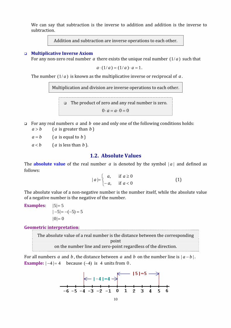
Geometric interpretation:
The absolute value of a real number is the distance between the corresponding point
on the number line and zero‐point regardless of the direction.
For all numbers a and b , the distance between a and b on the number line is || ba − . Example: 4|4| =− because )4(− is 4 units from 0 .

11
Properties of absolute values
0|| ≥a 0|| =a if and only if 0=a |||||| baba ⋅=⋅
||||||
ba
ba= ( 0≠b )
|||| aa =− |||| abba −=− 22|| aa =
1.3. Fractions
A fraction is a number written in the form ba , where numbera is called a numerator and
number b is called a denominator. Both the numerator and denominator are any real numbers, but the denominator cannot be equal to zero. The fractions have the following properties:
The fraction keeps its value when both the numerator and denominator
are multiplied or divided by the same nonzero number:
ba
bcac
=
We can use this property to simplify the fraction by factoring the numerator and denominator into prime factors and reducing common factors. Examples:
• 32
533532
4530
=⋅⋅⋅⋅
= • 34
)12(3)12(4
3648
=−−
=−−
xx
xx
One can also read this property from left to right when it is necessary to reduce a fraction to
a different denominator, e.g. 108
2524
54
=⋅⋅
= .
In order to add (or subtract) fractions with the same denominators, combine the numerators and keep the same denominator:
bca
bc
ba +
=+ b
cabc
ba −
=−
Two last formulas can be combined into the following uniform expression:
bca
bc
ba ±
=±
12
In order to add (or subtract) fractions with unlike denominators, reduce the fractions to a common denominator by finding a common multiple of both denominators and then add (or subtract) the fractions with the same
denominators:
bdbcad
bdbc
bdad
dc
ba ±
=±=±
Examples:
• 152
151012
5352
3534
32
54
=−
=⋅⋅
−⋅⋅
=− • abc
acabca
abcc
bcab+
=+=+11
The numerator of a product of fractions equals the product of the numerators, and the denominator is equal to the product of the denominators of all the fractions:
bdac
dc
ba
=⋅
In order to divide two fractions, invert the second fraction to make the multiplication problem, then multiply:
bcad
cd
ba
dc
ba
==
Example: 5
235
635
6356 a
babb
ba
bba
=⋅
=⋅=
Equivalent fractions are known as proportions. If two ratios are equal, then their reciprocals are also equal:
dc
ba= ⇒
cd
ab=
The proportions may be solved by cross multiplication using the cross product property:
dc
ba= ⇒ bcad =
From dc
ba= it also follows that
ac
bd= and
db
ca= .
One can easily prove the following helpful property of proportions:
For any real numbers 1t and 2t that are not equal to zero at the same time, if λ==dc
ba
then λ=++
dtbtctat
21
21 .
It looks in a general form as follows:
13
If λ====n
n
ba
ba
ba ...
2
2
1
1 then λ=++++++
nn
nn
btbtbtatatat
...
...
2211
2211 .
Example:
• If wz
yx= , then
wyzx
wyzx
yx
55
7272
++
=−−
= .
All the above properties hold true for the quotient of two algebraic expressions. They usually apply for manipulations with rational expressions.
1.4. Sets
A set is a finite or infinite collection of objects. The objects are called elements or members of the set. For instance, numbers or words can be considered as elements. Capital letters are usually used as names for sets. The pair of braces, }{ , is used to enclose either elements of the set or its description list, using commas to separate the individual elements. If the set A is defined by the list of its elements, then it can be written in the following format:
elements} of{list=A If the element x is an element of a set A , it is written using the symbol Ax∈ . Otherwise, the statement “ x is not an element of A ” is written symbolically as Ax∉ . The set A can be also defined by describing its elements through characterizing properties: “The set A of all elements x such that x has the property P ”. In this case, the symbol “|” is used instead of the statement “such that”, and the set is written in the following format:
{ }PxA |= Examples: • Let A be a set of the elements bax ,, . The set A is defined here by the list of its elements
and so it can be denoted as },,{ xbaA = . • Let N be the set of all natural numbers: }...,3,2,1{=N
Then the notation N∈7 means that number seven is a natural number, and the notation N∉3 means that 3 is not a natural number.
• Let B be the set of the natural numbers except number five. Then B may be symbolized as
}5,|{ ≠∈= nNnnB .
Note: The set A is a finite set whereas N and B are infinite sets. If a set has no elements, it is called a null set or an empty set and it is denoted by the symbol Ø. Thus, the set of natural numbers 1<n is a null set: Ø} 1 nN,n|n{ =<∈ .
1.4.1. Some Important Sets
♦ The set of natural numbers N :
s}# {nat.s}# {Natural
}...,3,2,1{
===N
♦ The set of all integers is denoted by I :
s}#Integer {}...,2,1,0,1,2...,{
=−−=I
14
♦ The set of all rational numbers is symbolized as
s}# {RationalI} q p, 0,q |{p/qQ
=∈≠=
♦ The set of all irrational numbers is denoted by the symbol H .
♦ The set of all rational and irrational numbers is the set of real numbers that is denoted by the symbol R . The set of real numbers is also called the continuum.
1.4.2. Comparison between Sets
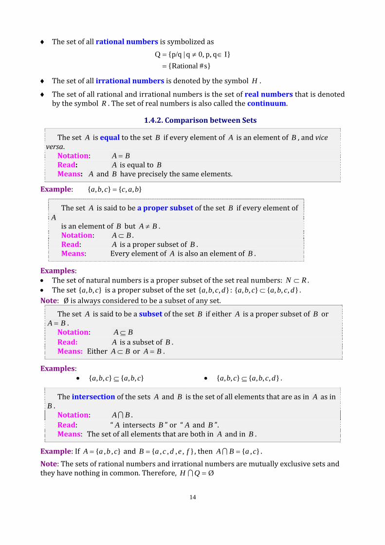
The set A is equal to the set B if every element of A is an element of B , and vice versa.
Notation: BA = Read: A is equal to B Means: A and B have precisely the same elements.
Example: },,{},,{ baccba =
The set A is said to be a proper subset of the set B if every element of A
is an element of B but BA ≠ . Notation: BA ⊂ . Read: A is a proper subset of B . Means: Every element of A is also an element of B .
Examples: • The set of natural numbers is a proper subset of the set real numbers: RN ⊂ . • The set },,{ cba is a proper subset of the set },,,{ dcba : },,,{},,{ dcbacba ⊂ . Note: Ø is always considered to be a subset of any set.
The set A is said to be a subset of the set B if either A is a proper subset of B or BA = . Notation: BA ⊆ Read: A is a subset of B . Means: Either BA ⊂ or BA = .
Examples: • },,{},,{ cbacba ⊆ • },,,{},,{ dcbacba ⊆ .
The intersection of the sets A and B is the set of all elements that are as in A as in B . Notation: BAI . Read: “ A intersects B ” or “ A and B ”. Means: The set of all elements that are both in A and in B .
Example: If },,{ cbaA = and },,,,{ fedcaB = , then },{ caBA =I . Note: The sets of rational numbers and irrational numbers are mutually exclusive sets and they have nothing in common. Therefore, Ø=QH I

15
The union of the sets A and B is the set of all elements that are either in A or B , or both.
Notation: BAU Read: “ A union B ” or “ A or B ”. Means: The set comprising all elements from A or B .
Example: s}# {rationals}# l{irrationas}# {real U= .
The Venn diagrams below illustrate the above definitions graphically.
1.5. Intervals
Intervals are special subsets of real numbers. An interval may be finite or infinite. The finite interval of real numbers lies between two real points, a and b . The infinite interval has only one real endpoint and contains all of the other real numbers that lie in the direction of positive or negative infinity from this point. ♦ If a collection of real numbers lies between a and b , but does not include either of
them, the interval is open. The open interval ),( ba is a set of all real numbers x with bxa << .
♦ If both endpoints, a and b , are included in the set, the interval is closed. The closed interval ],[ ba is a set of all real numbers x with bxa ≤≤ . Open and closed intervals are shown on the number line (Fig. 3a).
♦ A halfopen interval contains either a or b .
The half‐open interval ],( ba is a set of real numbers x with bxa ≤< , while ),[ ba is a set of real numbers x with bxa <≤ . Half‐open intervals look on the number line as the following (Fig. 3b):
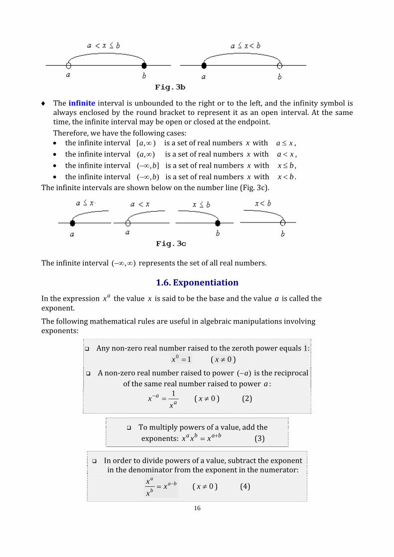
16
♦ The infinite interval is unbounded to the right or to the left, and the infinity symbol is always enclosed by the round bracket to represent it as an open interval. At the same time, the infinite interval may be open or closed at the endpoint. Therefore, we have the following cases: • the infinite interval ),[ ∞a is a set of real numbers x with xa ≤ , • the infinite interval ),( ∞a is a set of real numbers x with xa < , • the infinite interval ],( b−∞ is a set of real numbers x with bx ≤ , • the infinite interval ),( b−∞ is a set of real numbers x with bx < .
The infinite intervals are shown below on the number line (Fig. 3c).
The infinite interval ),( ∞−∞ represents the set of all real numbers.
1.6. Exponentiation
In the expression ax the value x is said to be the base and the value a is called the exponent. The following mathematical rules are useful in algebraic manipulations involving exponents:
Any non‐zero real number raised to the zeroth power equals 1: 10 =x ( 0≠x )
A non‐zero real number raised to power )( a− is the reciprocal of the same real number raised to power a :
aa
xx 1
=− ( 0≠x ) (2)
To multiply powers of a value, add the exponents: baba xxx += (3)
In order to divide powers of a value, subtract the exponent in the denominator from the exponent in the numerator:
bab
ax
xx −= ( 0≠x ) (4)

17
In order to raise powers of a value by a power, multiply the exponents: abba xx =)( (5)
A power of a product is equal to the product of powers: aaa yxxy =)( (6)
The numerator and denominator are raised to the power when raising a fraction to the power.
a
aa
yx
yx
=⎟⎟⎠
⎞⎜⎜⎝
⎛ ( 0≠y ) (7)
Examples:
• 2653653 / xxxxx == −+
• x
xxxx 1
)(1)6(7
32
7=== −−−−
−
−
• 409622)2( 124343 === ⋅
• 1)( 01141511
453=== −−
−
xxx
xx
1.6.1. Rational Exponents
The following is the definition of a radical in which the index n is a natural number greater than one: Nn∈ , 1>n . Number y is said to be the nth root of a real number x if xyn = .
The nth root of x is denoted symbolically by n x or nx1
. Thus, the relationship between exponents and roots is written as follows:
nxxn1
= (8) In the above expression x is known as the radicand, n is the index of the radical sign . Therefore, both equalities, xyn = and n xy = , express the same statement. The second root of a number is known as its square root, while its third root is known as its cube root. If the index n is equal to two, it can be omitted from the expression, i.e. the square root of the number x is written as 2 xx ≡ . The roots of real numbers may be either real or complex numbers. In particular, the nth root of a negative radicand, where n is even, has to be a complex number, since the nth power of any real number, where n is even, has to be a positive number. We will restrict our discussion of exponents and roots to real‐number solutions. No real nth root exists when the index n is even and the radicand x is a negative number. There are two real nth roots, y and )( y− , when the index n is even and the radicand is positive, because in this case nn yy )(−= . To avoid confusion, we define the principal nth root of a real number, where the nth root is a real number, to be the positive nth root of the number. When an algebraic expression refers to the nth root of a number, and the root is a real number, we generally mean by default the principal (positive) nth root of that number. For instance, the symbol x is defined for 0≥x and means the positive square root of the number x .
18
Therefore, ||2 xx = (9)
Examples: • Since 25)5(5 22 =−= , the square root of 25 has the values 5 and )5(− . Its positive
square root is 5 . Therefore, the principal square root of 25 is number 5 .
• 3|3|32 == , 3|3|)3( 2 =−=− . In order to find a square root we can factor an expression under the radical sign to get a perfect square. Then the perfect square is taken out from under the radical sign. What is not a perfect square is left under the radical sign.
Examples: 343431648 2 =⋅=⋅= .
The following properties of radicals are based on the rules of exponentiation and the properties of real numbers:
By setting na 1= and mb = , we get from rule (5):
nmmnnm
xxx11
)()( ==
Therefore, we have the following formula for radicals: mnn m xx )(= (10)
If we set a and b to be equal to )1( n , then from rule (6) it follows that:
nnn yxxy111
)()()( =
Hence, the nth root of a product of numbers is equal to the product of the nth roots: nnn yxxy ⋅= (11)
Similarly to above, the nth root of a quotient of two numbers is equal to the quotient of the nth roots:
n
nn
yx
yx= ( 0≠y ) (12)
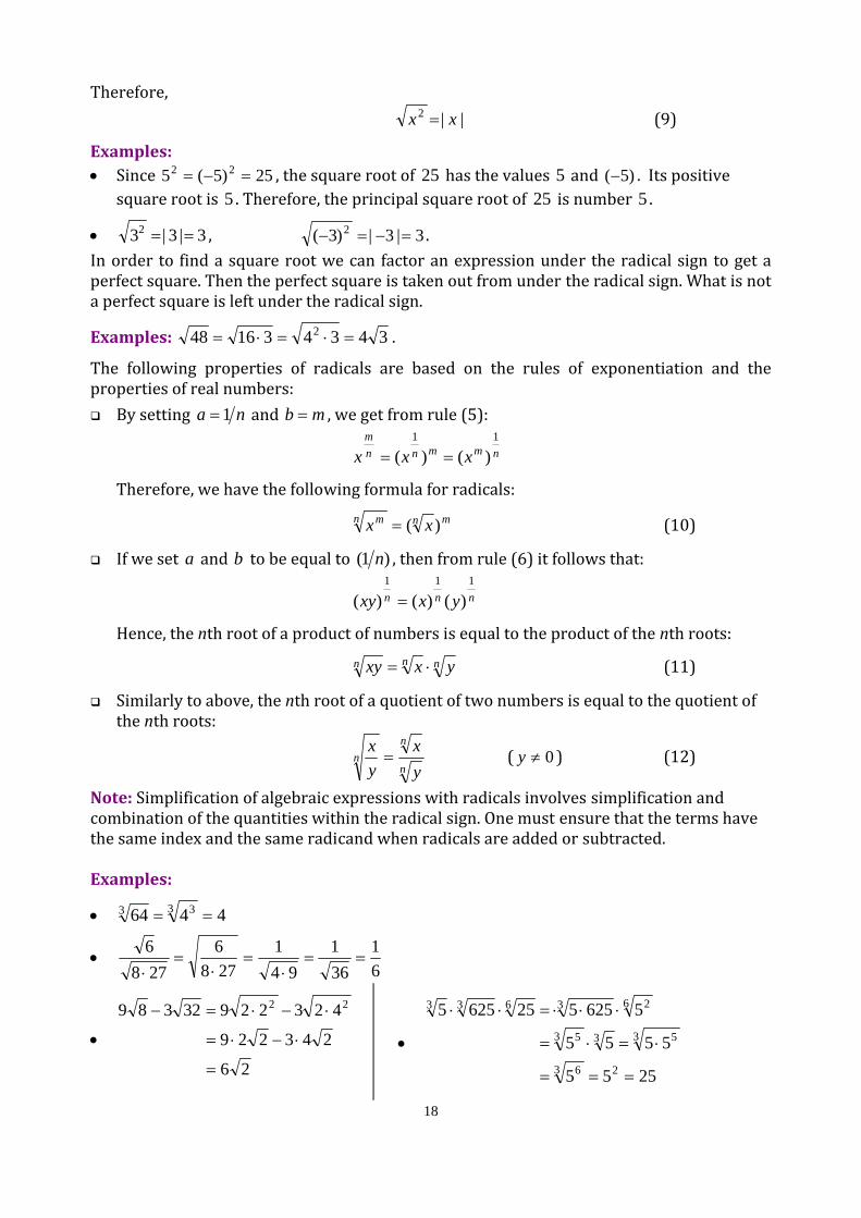
Note: Simplification of algebraic expressions with radicals involves simplification and combination of the quantities within the radical sign. One must ensure that the terms have the same index and the same radicand when radicals are added or subtracted. Examples:
• 4464 3 33 ==
• 61
361
941
2786
2786
==⋅
=⋅
=⋅
•
26
243229
42322932389 22
=
⋅−⋅=
⋅−⋅=−
•
2555
5555
56255256255
23 6
3 533 5
6 23633
===
⋅=⋅=
⋅⋅⋅=⋅⋅

19
1.6.2. Summary The most important rules of exponentiation are represented by the following table:
10 =x
aa
xx 1
=− 0≠x
baba xxx +=
bab
ax
xx −= 0≠x
abba xx =)(
aaa yxxy =)(
a
aa
yx
yx
=⎟⎟⎠
⎞⎜⎜⎝
⎛ 0≠x
nxxn1
=
||2 xx =
mnn m xx )(=
nnn yxxy ⋅=
n
nn
yx
yx= 0≠x
Algebra: Algebraic Expressions
20
2. Algebraic Expressions
♦ A constant is a symbol that represents a definite mathematical quantity.
♦ A variable is a symbol used to represent an unknown number.
♦ The number that the variable represents is called its value.
♦ A term is a product with an unspecified number of factors, where the factors are variables or constants.
♦ The variables of a term are said to be literal factors, and the product of the constants is called a coefficient of the term.
♦ The term, whose only factors are constants, is called a constant term.
♦ Terms that have the same literal factors but differ only in their numerical coefficients are called similar terms.
♦ The degree of a term in one variable is the exponent of that variable.
♦ An algebraic expression is an additive combination of any number of terms. By applying the distributive property, two or more similar terms can be combined into one term. The new term has the same literal factors as the similar terms, but its coefficient is the sum of the coefficients of the similar terms. This process is known as combining similar terms.
♦ The algebraic expression takes on a numerical value when numbers substitute for variables. This process is known as evaluating algebraic expression.
Example: • The algebraic expression
xxxyx 98354 23 −++− involves the terms xxxyx 9,3,5,4 23 −− and constant 8. The degree of the term 34x is 3. Two terms, x3 and )9( x− , have the same literal factor, so they are similar terms and can be combined into the single term )6( x− . The given expression is reduced to the following: 8654 23 +−− xxyx and can be evaluated by setting, e.g. 2=x and 3=y :
64812903282632524 23 −=+−−=+⋅−⋅⋅−⋅
♦ A term is called a monomial when its every variable has a non‐negative integer exponent.
♦ The degree of a monomial is the sum of the exponents of its variables. For example, the degree of the monomial 425 yx is (2+4)=6.
2.1. Polynomials
♦ The finite additive combination of monomials is known as a polynomial. We can say that a monomial is a polynomial with just one term.
♦ A polynomial with two terms is called a binomial; and a polynomial with three terms is a trinomial.
♦ The degree of a polynomial is the degree of the monomial with the highest degree.

Algebra: Algebraic Expressions
21
Examples: • The polynomial zx35 is a monomial of degree 4)13( =+ .
• The polynomial yx 92 − is a binomial of degree 1.
• The polynomial 3242 543 zyyzxx −+ is a trinomial. The term x3 has degree 1, the term 424 yzx has degree 7)412( =++ , and the term
)5( 32 zy− has degree 5)32( =+ . Thus, the above polynomial is the trinomial of degree 7.
A polynomial is one of the most important functions in mathematics and its applications. We can easily manipulate or evaluate the polynomial, but finding its roots is a more difficult task. There is a worthwhile case when a polynomial has a single variable. We will come to nothing more than polynomials with a single variable that are the most useful. A polynomial with a single variable is an expression that can be written in the following form:
011
1 ...)( axaxaxaxP nn
nn ++++= −
− (1)
where Nn∈ and x is a variable. The numbers na are called the coefficients; 0a is the constant coefficient.
A polynomial is said to be having degree n if 0≠na .
A polynomial is said to be a monic polynomial if the coefficient of the term of highest degree is one.
Examples:
• The polynomial 2)( =xP has degree 0; it is a constant polynomial.
• The polynomial 75)( += xxP has degree 1; it is a linear polynomial.
• The polynomial 43)( 2 +−= xxxP has degree 2; it is a quadratic polynomial.
• The polynomial 12)( 3 −+= xxxP has degree 3; it is a cubic polynomial.
Polynomials are not always given in an expanded form as above. For instance, the expression )1)(4( 2 +− xx is also a polynomial of degree 3, as it can be easily checked.
2.2. Algebraic Transformations
It is a general situation when one needs to write a particular algebraic expression in the simplest possible form. Although it is difficult to say exactly what one means in all cases by the "simplest form", a worthwhile practical procedure is to look at many different forms of an expression, and pick out the one that involves the smallest number of parts. There are many different ways to write the same algebraic expression. In most cases, it is best simply to experiment, trying different transformations until we get a suitable form. It is impossible to formulate any general‐purpose method of getting expressions into the simplest form. For instance, if one has an expression with a single variable, one can choose to write it as a sum of terms, a product, and so on.

Algebra: Algebraic Expressions
22
When one has an expression with several variables, there is an even wider selection of possible forms. One can, for example, group terms in the expression in such a way that one or another of the variables is chosen as major. Even when we deal with polynomials and rational expressions, there are many different ways to write any particular expression. If we consider more complicated expressions, involving, for example, trigonometric functions, the variety of possible forms becomes still greater. However, we can try to formulate some simple principles that are suitable for solving some specific tasks. First of all let us define the following common rules: • Perform a sequence of algebraic transformations on the expression and return to the
simplest form you found. • Simplify the expression making use of factoring or expanding of some parts of
expression. • Collect together terms that involve the same powers or radicals, etc. • Put all terms over a common denominator or separate into terms with simple
denominators. • Cancel common factors between the numerator and denominator, etc. Here we consider the following common and useful methods of manipulating and simplifying algebraic expressions, equations and inequalities: factoring, expanding and rationalizing the denominator.
2.2.1. Factoring
“Factor expression” is the same as “write expression as a product of factors”. This procedure often gives simpler expressions. As one example, the following expression
4232 )3()2)(( yxyxyx +−+ is the polynomial with two variables and 36 terms. As is known, the process of factoring a real number involves expressing the number as a product of prime numbers that are irreducible factors, i.e. each of which has only two factors, the number one and the prime number itself. Similarly, we can factor a polynomial expression by representing it as a product of irreducible polynomials, i.e. the polynomials each of which cannot be further reduced to other factors aside from the number one and itself. Transformations of expressions by expanding or factoring are always correct, whatever values the symbolic variables in the expressions may have. Examples: Factor the following expressions to irreducible factors:
• 532260 ⋅⋅⋅= • )25(3615 2 aaaa −=− • )3)(2()2(3)2(6322 −+=+−+=−−+ abababaabaaba
Problem 1: Reduce to a product of factors the difference between two squares: 22 ba − . Solution: First, we subtract and add the product ab :
2222 babababa −+−=−
Then, we combine the terms by pairs and take out the common factors:
))(()()(22
babababbaabababa
+−=−+−=−+−
Algebra: Algebraic Expressions
23
Finally, we get the following helpful formula:
))((22 bababa +−=− (2)
Examples:
• )53)(53(5)3(259 222 +−=−=− xxxx
•
)13)(3((3)39)(3(
)435)(435()4()35(16)35( 2222
++=++=
++−+=−+=−+
xxxx
xxxxxxxx
• )1)(1)(1()1)(1(1)(1 2222224 ++−=+−=−=− xxxxxxx
•
)21)(21(
)2()1(
2)12)((
2121
22
222
2222
2244
xxxx
xx
xxx
xxxx
++−+=
−+=
−++=
−++=+
Problem 2: Reduce to a product of factors the following quadratic polynomial: 22 2 baba ++
Solution: First, we rewrite the term ab2 as abab + ; next, we combine the terms by pairs; then, we take out the common factors:
))(()()()()(
222
2222
babababbaabababa
bababababa
++=+++=+++=
+++=++
Finally, we obtain the following formula for the perfect square: 222 2)( bababa ++=+ (3)
Corollary: From the last formula one can easily get another formula for the perfect square by substituting )( b− for b :
222 )()(2))(( bbaaba −+−+=−+ ⇒
222 2)( bababa +−=− (4)
Formulas (3)‐(4) can now be combined into a uniform formula: 222 2)( bababa +±=± (5)
Problem 3: Reduce to a product of factors the difference between two cubes: 33 ba − Solution: We can use a similar way as above, but now we first add and subtract the terms
ba2 and 2ab ; then we combine the terms by pairs and take out the common factors:
Algebra: Algebraic Expressions
24
))((
)()()(22
22
32222333
bababa
babbaabbaa
bababbabaaba
++−=
−+−+−=
−+−+−=−
We have one more helpful formula:
) bab b) (a (a ba 2233 ++−=− (6)
Corollary: From the last formula one can easily get a formula for the sum of two cubes by substituting )( b− for b :
)2233 (-b)(-b) a (-b)) (a (a (-b)a +⋅+−=− ⇒
) bab b) (a (a ba 2233 +−+=+ (7)
Examples:
•
)41025)(25(
))2(255)(25(
)2(58125
2
22
333
xxx
xxx
xx
++−=
+⋅+−=
−=−
• )41025)(25()2(58125 2333 xxxxx +−+=+=+
•
11
11)1(
1)1(
1)12(
11
)1)(1()1)(1(
11
22
22
2
2
3
+−+=
+−
++
=+
−+=
+−++
=+++
=
+−++−
=−−
xxx
xx
xx
xxx
xxxx
xxx
xxxxx
xx
2.2.2. Expanding
Here we consider one more method of transformation between different forms of algebraic expressions. Expanding is the inverse operation to factoring. We can get another form of an algebraic expression if we multiply out products and powers, writing the result as a sum of terms. We give below some examples. Examples: We can also read formulas (3)‐(5) from right to left and expand the following expression:
• 11025152)5()15( 222 +−=+⋅−=− xxxxx
• 422222222 9124)3(322)2()32( yxyxyyxxyx ++=+⋅⋅+=+
• 2222 16249)4(4323)43( xxxxx +±=+⋅⋅±=±
Problem 4: Prove the following formulas: 32233 33)( babbaaba +++=+ (8)
32233 33)( babbaaba −+−=− (9)
Algebra: Algebraic Expressions
25
Proof: Let us start from the cube of sum (8) and expand the expression on the left‐hand side:
3223
32223
22
23
33
2
))(2(
)()()(
babbaa
bababbaa
bababa
bababa
+++=
++++=
+++=
++=+
Then, as above, we get a formula for the cube of the difference by substituting )( b− for b :
3223
32233
33
)()(3)(3)(
babbaa
bbabaaba
−+−=
−+−+−+=−
Excellent advice: Memorize and use the above formulas. Examples:
• 442
3222332
125150608
)5()5(235232)52(
xxx
xxxx
+++=
+⋅⋅⋅+⋅⋅+=+
• 2223
22233
125150608
)5()5(235)2(3)2()52(
babbaa
bbabaaba
−+−=
−⋅+⋅−=−
2.2.3. Rationalizing Denominators
Since a rational expression is the quotient of two algebraic expressions, it can be represented in a fractional form. In doing so, it is often desirable to eliminate all the terms involving radicals from the denominator of the fraction. This is known as rationalizing the denominator. Examples:
• ||22 b
ab
b
abbab
ba
===
• 5
5255
525
2==
• 1133
11
331133
113
22 ===
There are tree cases when the denominator can be easily rationalized. 1. Let the denominator be a binomial radical expression )( ba + , where each item, a and b
, can contain radicals, but the difference between two squares, 22 ba − , cannot do so. Then one can multiply both the numerator and denominator of the fraction by factor
)( ba − to rationalize the denominator (in view of formula for the difference between two squares):
22))((1
baba
bababa
ba −−
=−+
−=
+ (10)
Example: Rationalize the denominator of the given expression: )32(
1−
.
Algebra: Algebraic Expressions
26
Solution: First, we multiply both the numerator and the denominator by the factor )32( + . Then we use the formula (2):
323432
)3(232
)32)(32(32
321
22 +=−+
=−+
=
+−+
=−
Example: Rationalize the denominator of the given expression: )12(1 + . Solution: Now we multiply both the numerator and the denominator by the factor )12( − and end up by using formula (2):
121212
1)2(12
)12)(12(12
121
2 −=−−
=−
−=
−+−
=+
Example: Rationalize the denominator of the given expression:
153151
−+−.
Solution: First of all we have to factor the denominator. Making use of the identity 3515 = , one can combine the terms by pairs and take out the common factor:
)13)(15()15()15(3
1533515315
+−=−+−=
−+−=−+−
Now the fraction can be represented as a product of the fractions:
131
151
153151
+⋅
−=
−+−
so that each of them, taken separately, can be rationalized as above:
)13)(15(81)13(
21)15(
41
)13)(13(13
)15)(15(15
131
151
−+=−+=
−+−
⋅+−
+=
+⋅
−
Example: Rationalize the denominator of the given expression: 2)57(
1
+
Solution: First, we rationalize the denominator of the fraction )57(1 + :
)57(21
5757
)5()7(57
)57)(57(57
571
22 −=−−
=−−
=
−+−
=+
which being squared gives:
2353)53527(
41
))5(572)7((41
)57(1 22
2
−=+−=
+−=+
Algebra: Algebraic Expressions
27
Example: Rationalize the denominator of the given expression: 1212
−+
Solution: As above, we first rationalize the denominator of the fraction )12(1 − :
121212
)12)(12()12(
121
+=−+
=+−
+=
−
Then, we multiply the above by the term )( 12 + and take a square root:
12)12(1212 2 +=+=
−+
2. Now let the denominator be a trinomial radical expression with the structure )( 22 baba ++ , where each item can contain radicals, but the difference between cubes,
33 ba − , cannot do so. Then the problem of rationalizing the denominator is solved in a similar way: we multiply both the numerator and denominator of the fraction by the factor )( ba − and use the formula for the difference between two cubes:
332222 ))((1
baba
babababa
baba −−
=−++
−=
++ (11)
3. Let the denominator be a trinomial radical expression with the structure )( 22 baba +− , where each item, but not the sum of cubes, 33 ba + , can contain radicals. Then we have a similar problem, so it can be solved as above:
332222 ))((1
baba
babababa
baba ++
=++−
+=
+− (12)
The below examples involve the cases when a denominator can be rationalized by using the formulas for the sum and difference of two cubes in view of the properties of radicals. Examples:
•
6945
64545
4)5(45
)45)(454)5((45
454)5(1
1654251
33
333
3
32323
3
232333
+=
++
=++
=
++−+
=
+−=
+−
•
yxyx
yxyx
yxyyxxyx
yxyx
−−
=−
−=
−+⋅+−
=++
33
3333
33
33233323
33
3 233 2
)()(
))()()((1
We can also use formulas (11)‐(12) to solve similar problems. Example: Rationalize the denominator of the given expression: )42(1 33 2 ++ xx . Solution: Setting 3 xa = and 2=b we get from formula (11) the following result:
82
42
1 3
33 2 −−
=++ x
x
xx.

Algebra: Algebraic Expressions
28
3. Algebraic Equations and Inequalities ♦ An algebraic equation is a mathematical statement of the equivalence (in a certain
well‐defined sense) of two algebraic expressions, i.e. it states that one algebraic expression is equal to another algebraic expression.
♦ An algebraic inequality is a mathematical statement comparing two algebraic expressions. One algebraic expression can be • greater than (>) another; • less than (<) another; • greater than or equal to )(≥ another; • less than or equal to )(≤ another algebraic expression.
The symbols ba << and ba >> are used to denote “ a is much less than b '' and “ a is much greater than b ”, respectively.
♦ The solution of equations and inequalities involves finding the values of the variables that make the mathematical statements true. The addition and multiplication properties of equalities and inequalities as well as the properties of real numbers, are used to simplify the equation or the inequality as much as possible, prior to formulating the solution set for the variable in question.
3.1. Properties of Equations and Inequalities
The following properties of equalities apply to equations. The addition property of equalities states that
ba = if and only if cbca +=+ for any c .
This property applies to equations, but it is better to say:
Any number or expression can be added to both sides of an equation to produce an equivalent equation.
The multiplication property of equalities states that ba = if and only if bcac = for any 0≠c .
A more suitable wording for equations is the following:
Both sides of an equation can be multiplied by the same non‐zero quantity to produce an equivalent equation.
The addition property of inequalities states that ba > if and only if cbca +>+ for any c .
In other words:
Any number or expression can be added to both sides of an inequality to produce an equivalent inequality.
The multiplication property of inequalities is given in two cases. The first case states that
if ba > and 0>c then bcac > .
Algebra: Algebraic Expressions
29
The second case states that if ba > and 0<c then bcac < .
Both sides of an inequality can be multiplied by the same positive quantity to produce an equivalent inequality:
If both sides of an inequality are multiplied by the same negative quantity, then the inequality symbol must be reversed:
3.2. Linear Equations
A linear equation in one variable is that equation which can be put into the following form:
0=+ bax (1)
where a and b are constants ( 0≠a ), and x is a variable. Let us note that the expression on the left‐hand side (1) is a linear polynomial. Here is the solution of the equation (1):
abx −= (2)
Example: Solve the equation 2211 bxabxa +=+ for the variable x . Solution: In order to solve the given equation, first we have to subtract xa2 and 1b from both sides.
1221 bbxaxa −=− Next, we combine similar terms: 1221 )( bbxaa −=−
If 21 aa ≠ , then the solution is 21
12
aabbx
−−
= .
If 21 aa = and 21 bb = , then the solution set is any Rx∈ . If 21 aa = but 21 bb ≠ , then the given equation has no solution.
3.3. Linear Inequalities
A linear inequality in one variable is that inequality which can be put into one of the following forms:
0≥+ bax (3a) 0>+ bax (3b)
where a and b are constants ( 0≠a ), and x is a variable. • If 0>a , then the solution set is respectively
abx −≥ (4a) abx −> (4b)
• Otherwise, if 0<a , then the solution set is
abx −≤ (5a) abx −< (5b)
The endpoint of the solution's interval may be included or not. It depends on whether the inequality contains the inequality symbol “≥ ” (“≤ ”) or “>” (“<”).
Algebra: Algebraic Expressions
30
The process of solving inequalities is similar to that of equations, except that properties of inequalities apply. Example: Solve the following inequality: 17235 +≥+− xx Solution: First, we have to simplify this inequality by subtracting the term x2 and the number 3 from both sides:
147 ≥− x . Then we divide both sides of the above inequality by the negative number )7(− to get the solution set: 2−≤x
3.4. Linear Equations Involving Absolute Values
1. Let a linear equation involve some absolute value || bax + . Following the definition of an absolute value, we can drop the absolute symbol, provided that the correct sign is chosen. There are two possible cases: 1) if 0≥+ bax , then baxbax +=+ || ; 2) if 0<+ bax , then )(|| baxbax +−=+ . Therefore, the initial equation is split into two equations such that each of them does not contain the absolute value bars. Hence, we must solve two ordinary linear equations and choose solutions to satisfy the above conditions.
Example 1: Solve the equation 5|32| =+x Solution: Case 1: If 032 ≥+x , that means 23−≥x , then the absolute symbol can be simply dropped:
5|32| =+x ⇒ 532 =+x ⇒ 1=x , provided that 23−≥x . That is a true statement.
Case 2: If 032 <+x , that means 23−<x , then we have to change the sign in front of the expression )52( +x when the absolute symbol is dropped:
5|32| =+x ⇒ 5)32( =+− x ⇒ 4−=x , provided that 23−<x . That is true. The solution set is the union of the solutions involving case 1 and case 2:
}1,4|{ =−= xxx .
Example 2: Solve the equation 1|152| =+x Solution:
Case 1: If 0152 ≥+x , that means 2
15−≥x , then
1|152| =+x ⇒ 1152 =+x ⇒ 7−=x , provided that 2
15−≥x .
That is certainly true.
Case 2: If 0152 <+x , then 1)152( =+− x ⇒ 4−=x , provided that 2
15−<x .
That is a contradiction, since )215()4( −>− . Therefore, the value 4−=x is not the solution for the considered equation, i.e. the solution set for case 2 is the empty set Ø. Hence, the solution set involves the singular value 7−=x .

Algebra: Algebraic Expressions
31
2. When an equation involves absolute values || bax + and || dcx + , then we have to make a few steps to solve the equation: • Solve each intermediate equation below for x to find out where the expressions
change their signs: 0=+ bax ⇒ 1xx = 0=+ dcx ⇒ 2xx =
Let 1x be less than 2x . We use this statement for the sake of determinacy only because the opposite case can be considered in a similar way.
We get three intervals: ),( 1x−∞ , ),[ 21 xx and ),[ 2 ∞+x ;
hence, we have to solve three ordinary equations when absolute bars are dropped and correct signs of the expressions are applied. The positive or negative value of each expression must be
evaluated separately according to the definition of the absolute value. • It is necessary to select consistent solutions by testing whether each solution lies in the
corresponding interval. The solution set is the union of the solutions involving all cases. Example 3: Solve the given equation
xxx 4|27||43| −−=+ (6) Solution: 1) We solve two intermediate linear equations:
043 =+x ⇒ 34
−=x
027 =−x ⇒ 72
=x
Thus, we have obtained the following three intervals: )34,( −−∞ , )72,34[− and ),72[ ∞+. 2) Now we consider three cases:
Case 1: If 34
−<x , then )43(|43| +−=+ xx and )27(|27| −−=− xx .
Hence, equation (6) can be transformed in the following way: xxx 4|27||43| −−=+ ⇒ xxx 42743 −+−=−− ⇒
68 =x ⇒ 43
=x , provided that 34
−<x .
That is a contradiction. Hence, the equation (6) has no solution when 34
−<x .
Case 2: If 72
34
<≤− x , then 43|43| +=+ xx and )27(|27| −−=− xx .
As above, we get the following result: xxx 4|27||43| −−=+ ⇒ xxx 42743 −+−=+ ⇒
214 −=x ⇒ 71
−=x , provided that 72
34
<≤− x .
That is true.
Algebra: Algebraic Expressions
32
Case 3: If 72
>x , then 43|43| +=+ xx and 27|27| −=− xx .
Hence, the equation (6) implies xxx 42743 −−=+ ⇒ 24 −= .
That is a contradiction and so equation (6) has no solution when 72
>x .
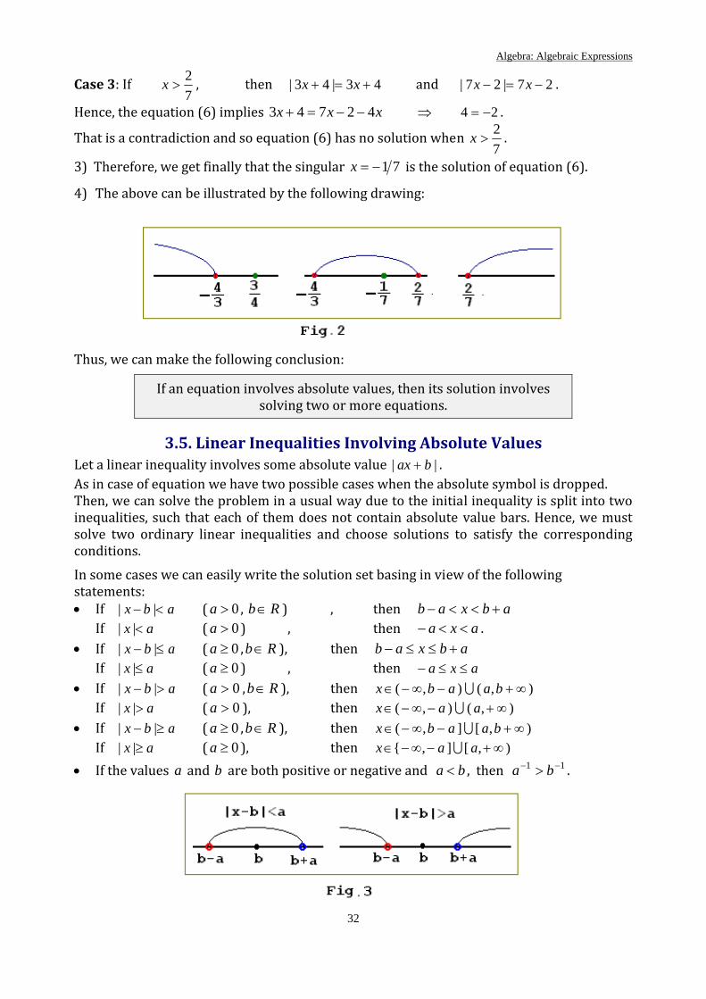
3) Therefore, we get finally that the singular 71−=x is the solution of equation (6).
4) The above can be illustrated by the following drawing:
Thus, we can make the following conclusion:
If an equation involves absolute values, then its solution involves solving two or more equations.
3.5. Linear Inequalities Involving Absolute Values Let a linear inequality involves some absolute value || bax + . As in case of equation we have two possible cases when the absolute symbol is dropped. Then, we can solve the problem in a usual way due to the initial inequality is split into two inequalities, such that each of them does not contain absolute value bars. Hence, we must solve two ordinary linear inequalities and choose solutions to satisfy the corresponding conditions. In some cases we can easily write the solution set basing in view of the following statements: • If abx <− || ( 0>a , Rb∈ ) , then abxab +<<−
If ax <|| ( 0>a ) , then axa <<− . • If abx ≤− || ( 0≥a , Rb∈ ), then abxab +≤≤−
If ax ≤|| ( 0≥a ) , then axa ≤≤− • If abx >− || ( 0>a , Rb∈ ), then ),(),( ∞+−∞−∈ baabx U
If ax >|| ( 0>a ), then ),(),( ∞+−∞−∈ aax U • If abx ≥− || ( 0≥a , Rb∈ ), then ),[],( ∞+−∞−∈ baabx U
If ax ≥|| ( 0≥a ), then ),[],{ ∞+−∞−∈ aax U • If the values a and b are both positive or negative and ba < , then 11 −− > ba .

Algebra: Algebraic Expressions
33
Example 1: Solve the inequality 5|13| <−x . Solution: According to the above statement it follows from the given inequality that
51351 +<<− x ⇒ 234
<<− x
Example 2: Solve the inequality 3|54| ≥+x . Solution: As above 3|54| ≥+x ⇒ )53(4 −−≤x or 534 −≥x ⇒ 2−≤x or )21(−≥x
Therefore, the solution set is ))21()2(|( −≥−≤ xxx U
Example 3: Solve the inequality xx 2|13| <− . Solution:
Case 1: If 013 ≥−x , that means 31
≥x , then
xx 2|13| <− ⇒ xx 213 <− ⇒ 1<x , provided that 31
≥x .
So the solution set in this case is )1,31[∈x .
Case 2: If 013 <−x , that means 31
<x , then
xx 2|13| <− ⇒ xx 2)13( <−− ⇒ 51
>x , provided that 31
<x .
Now the solution set is )31,
51(∈x .
One can easily find the union of the of the solutions involving cases 1 and 2:
)1,51(}1,
31[)
31,
51( =U
Therefore, xx 2|13| <− for any )1,51(∈=x .
Example 4: Solve the inequality 105|2| −≤+ xx . Solution:
Case 1: If 02 ≥+x , that means 2−≥x , then 105|2| −≤+ xx ⇒ 1052 −≤+ xx ⇒ 3≥x , provided that 2−≥x .
Hence, the solution set in this case includes any ),3[ ∞+∈x . Case 2: If 02 <+x , that means 2−<x , then
105|2| −≤+ xx ⇒ 105)2( −≤+− xx ⇒ 34
≥x , provided that 2−<x
. This case is impossible. Therefore, the solution set contains case 1 only: ),3[ ∞+∈x .
If an inequality involves two or more absolute values, then its solution involves solving three or more inequalities. Then, it is necessary to select the solutions obtained by testing whether each of them lies in the corresponding interval. The solution set is the union of the solutions involving all cases.
Algebra: Algebraic Expressions
34
3.6. Quadratic Equations
A quadratic equation in one variable x is that equation which can be written in the following form:
02 =++ cbxax (7)
where ba , and c are constants ( 0≠a ). Equation (7) is also said to be a second‐degree equation. We can see that the expression on the left‐hand side (7) is a quadratic polynomial. There is nothing special about the symbol x in these equations; any other letter could be used. The equation
02 =++ cbzaz is also a quadratic equation that is quadratic in one variable, namely, z . An expression is said to be a monic quadratic in a single variable x if it can be written as
acx
abx ++2 . Therefore, any quadratic equation in only one variable can be rewritten so
that one side is a monic quadratic by dividing both sides by the numerical coefficient of the quadratic term:
02 =++acx
abx (8)
There are a few methods of solving the second‐degree equations: • completing the square, • using the quadratic formula, • factoring.
3.6.1. Completing the Square
Let us transform the quadratic polynomial on the left‐hand side of equation (8) by adding and subtracting the constant to complete the perfect square:
))2
(()2
(
)2
()2
(
22
2222
ac
ab
abx
ac
ab
abx
abx
acx
abx
−−+=
+−++=++
We get the equation that is equivalent to the original one:
))2
(()2
( 22
ac
ab
abx −=+ .
Now we reduce the right side to a common denominator:
2
22
44)
2(
aacb
abx −
=+ (9)
The value acbD 42 −=
is said to be a discriminant of the quadratic equation. The sign of the discriminant is an important characteristic of the quadratic equation. There are tree possible cases: 0<D , 0=D and 0>D .
Case 1: If 0<D , then in view of equality (9) we get 0)2
( 2 <+a
bx .
This is a contradiction. Therefore, equation (8) has no real roots, i.e. the solution set for case 1 is the empty set Ø. Case 2: If 0=D , then from (9) we get
Algebra: Algebraic Expressions
35
0)2
( 2 =+a
bx
Therefore, equation (8) has one real root or rather two real roots that are equal to each other:
abx
2−= (10)
Case 3: If 0>D , then by taking the square root of the both sides, the equation (2) can be transformed into the following form::
aacb
abx
24|
2|
2 −=+ ⇒
aacbbx
242 −±−
= (11a)
Formula (11a) is known as quadratic formula. It gives the complete solution of the quadratic equation (7) and it is usually written as follows:
aDba
acbbx
2
242
2,1
±−=
−±−=
(11b)
Example 1: The equation 043 2 =+− xx has no real roots because the discriminant 059534)1( 2 <−=⋅⋅−−=D
Example 2: The equation 0962 =+− xx has the solution 326 ==x in view of formula (10) because 03636 =−=D . Example 3: The equation 0562 =++ xx has the solution set 1,5 21 −=−= xx in view of formula (11).
3.6.2. Factoring a Polynomial Expression
Another way to solve a quadratic equation is based on factoring a polynomial expression, i.e. by representing it as a product of irreducible polynomials. This worthwhile method is suitable for solving another kind of equations too.
• If 0<D , then equation (8) has no real roots, and polynomial acx
abx ++2 cannot be
reduced to other factors aside from the number one and itself. • If 0=D , then roots for equation (8) coincide with each other: 21 xx = . So the
considered polynomial can be represented as 2
12 )( xx
acx
abx −=++ (12)
• If 0>D , then equation (8) has two real roots 1x and 2x ( 21 xx ≠ ), i.e. the polynomial
acx
abx ++2 is equal to zero, if and only if either 1xx = or 1xx = . Among the second‐
degree polynomials there is only one, namely ))(( 21 xxxx −− , that has the same properties. Consequently,
))(( 212 xxxx
acx
abx −−=++ (13)
Algebra: Algebraic Expressions
36
Let us remove the parentheses on the right side of equation (13) and combine similar terms:
212122 )( xxxxxx
acx
abx ++−=++ ⇒
acxxxxx
ab
−=++ 2121 )(
This is a true statement when
021 =++ xxab and 021 =−
acxx .
Hence, the sum of the roots for the quadratic equation (8) produces the relationship
abxx −=+ 21 (14)
and the product of the roots produces the relationship
acxx =21 (15)
These helpful statements may be used to find the roots or check if the found roots are correct. Example 3: Solve the quadratic equation 01242 =−− xx . Solution: First, we add and subtract x2 to the left side of the equation, next group the terms by pairs, then take out the common factor: 01242 =−− xx ⇒ 0126)2( 2 =−−+ xxx ⇒
0)2(6)2( =+−+ xxx ⇒ 0)6)(2( =−+ xx A product of terms is equal to zero if only any of them equals zero. Hence, the solution set is
2−=x and 6=x . Example 4: Solve the quadratic equation 0542 =−+ xx . Solution: One can easily see that
)5(14 −+=− and )5(15 −⋅=− Hence, in view of relationships (7)‐(8) we get the solution set 5−=x and 1=x . Example 5: Solve the quadratic equation 024112 =+− xx . Solution: It is evident that
8311 += and 8324 ⋅= Hence, in view of relationships (7)‐(8) we get the solution set 3=x and 8=x . Check:
If 3=x , then 024112 =+− xx ⇒ 0243332 ≡+− . That is true. If 8=x , then 024112 =+− xx ⇒ 0248882 ≡+− . That is true.
Example 6: Solve the cubic equation 064 23 =−++ xxx . Solution: Let us transform the cubic polynomial on the left‐hand side of the equation. First, we subtract and add the term 22x . Next, we combine the terms by pairs. Then, we factor the obtained expression:

Algebra: Algebraic Expressions
37
)3)(2)(1()65)(1(
)66)(1(
)1)(1(6)1()1(
)1(6)1()1(
)66()()(64
2
2
2
22
222323
++−=++−=
++−−=
+−+−−−=
−+−−−=
−+−−−=−++
xxxxxx
xxxx
xxxxxx
xxxxx
xxxxxxxx
Thus, 0)3)(2)(1( =++− xxx . A product of terms is equal to zero if only any of the terms equals zero. Hence, the solution set is 2,3 −=−= xx and 1=x .
3.7. Quadratic Inequalities
A quadratic inequality in one variable is that inequality which can be put into one of the following forms:
02 >++ cbxax (16a) 02 ≥++ cbxax (16b)
where a , b and c are constants ( 0≠a ), and x is a variable.
In order to solve the quadratic inequality it is necessary first to solve the corresponding quadratic equation (7): 02 =++ cbxax .
There are three possible cases: 1. If 0<D , then equation (7) has no real roots, and the expression cbxax ++2 has the
same sign as the coefficient a for each value of x .
2. If 0=D , then roots for equation (7) coincide with each other: 21 xx = . So the expression cbxax ++2 has the same sign as the coefficient a for each value x except
21 xxx == when it is equal to zero.
3. If 0>D , then equation (7) has two real roots 1x and 2x ( 21 xx < ), so the polynomial cbxax ++2 changes its sign when the variable x jumps over 1x or 2x . Therefore, there
are three intervals: ),( 1x−∞ , ),( 21 xx and ),( 2 ∞x . • If 0>a , then the solution set for inequalities (16a)‐(16b) is respectively
}|{ 21 xxxxx >< U or }|{ 21 xxxxx ≥≤ U . • If 0<a , then the solution set for inequalities (16) is respectively
}|{ 21 xxxx << or }|{ 21 xxxx ≤≤ .
We can use the number line to get the solution set for the inequality.
Example 1: Solve the following inequality:
0822 >−+ xx (17)
Algebra: Algebraic Expressions
38
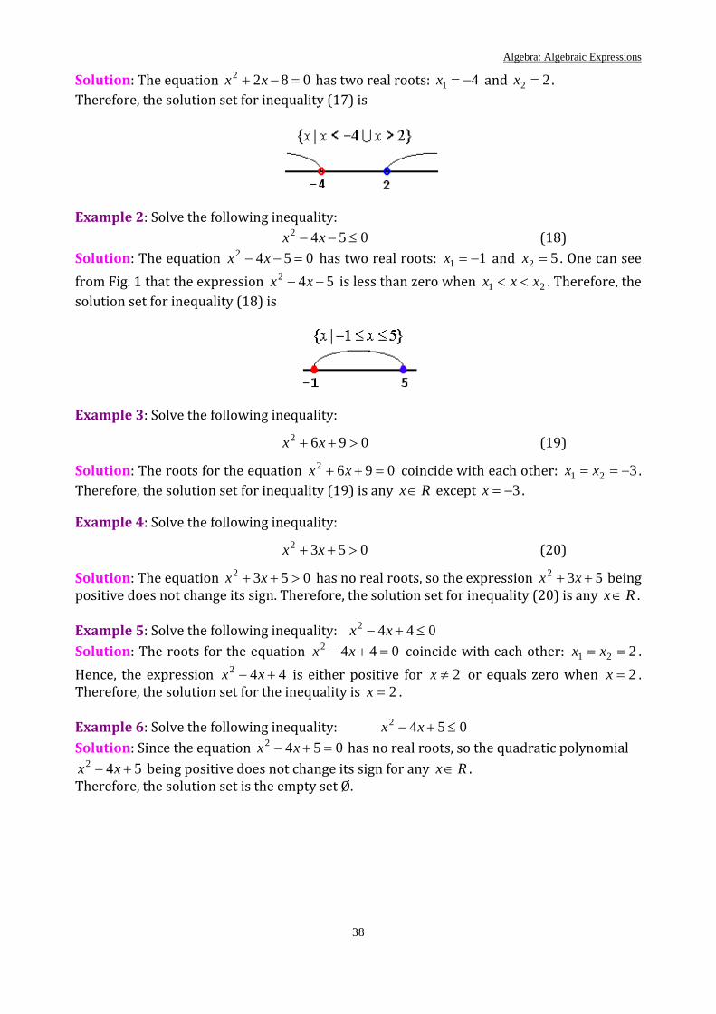
Solution: The equation 0822 =−+ xx has two real roots: 41 −=x and 22 =x . Therefore, the solution set for inequality (17) is
Example 2: Solve the following inequality: 0542 ≤−− xx (18)
Solution: The equation 0542 =−− xx has two real roots: 11 −=x and 52 =x . One can see from Fig. 1 that the expression 542 −− xx is less than zero when 21 xxx << . Therefore, the solution set for inequality (18) is
Example 3: Solve the following inequality:
0962 >++ xx (19)
Solution: The roots for the equation 0962 =++ xx coincide with each other: 321 −== xx . Therefore, the solution set for inequality (19) is any Rx∈ except 3−=x .
Example 4: Solve the following inequality:
0532 >++ xx (20)
Solution: The equation 0532 >++ xx has no real roots, so the expression 532 ++ xx being positive does not change its sign. Therefore, the solution set for inequality (20) is any Rx∈ .
Example 5: Solve the following inequality: 0442 ≤+− xx Solution: The roots for the equation 0442 =+− xx coincide with each other: 221 == xx . Hence, the expression 442 +− xx is either positive for 2≠x or equals zero when 2=x . Therefore, the solution set for the inequality is 2=x .
Example 6: Solve the following inequality: 0542 ≤+− xx Solution: Since the equation 0542 =+− xx has no real roots, so the quadratic polynomial
542 +− xx being positive does not change its sign for any Rx∈ . Therefore, the solution set is the empty set Ø.
Algebra: Functions
39
4. Functions
4.1. Introduction to Cartesian Coordinate System
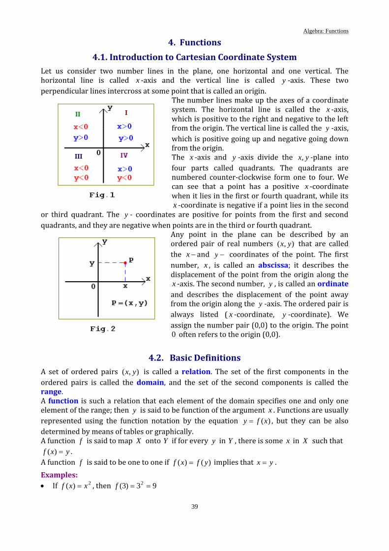
Let us consider two number lines in the plane, one horizontal and one vertical. The horizontal line is called x ‐axis and the vertical line is called y ‐axis. These two perpendicular lines intercross at some point that is called an origin.
The number lines make up the axes of a coordinate system. The horizontal line is called the x ‐axis, which is positive to the right and negative to the left from the origin. The vertical line is called the y ‐axis, which is positive going up and negative going down from the origin. The x ‐axis and y ‐axis divide the yx, ‐plane into four parts called quadrants. The quadrants are numbered counter‐clockwise form one to four. We can see that a point has a positive x ‐coordinate when it lies in the first or fourth quadrant, while its x ‐coordinate is negative if a point lies in the second
or third quadrant. The y ‐ coordinates are positive for points from the first and second quadrants, and they are negative when points are in the third or fourth quadrant.
Any point in the plane can be described by an ordered pair of real numbers ),( yx that are called the −x and −y coordinates of the point. The first number, x , is called an abscissa; it describes the displacement of the point from the origin along the x ‐axis. The second number, y , is called an ordinate and describes the displacement of the point away from the origin along the y ‐axis. The ordered pair is always listed ( x ‐coordinate, y ‐coordinate). We assign the number pair (0,0) to the origin. The point 0 often refers to the origin (0,0).
4.2. Basic Definitions
A set of ordered pairs ),( yx is called a relation. The set of the first components in the ordered pairs is called the domain, and the set of the second components is called the range. A function is such a relation that each element of the domain specifies one and only one element of the range; then y is said to be function of the argument x . Functions are usually represented using the function notation by the equation )(xfy = , but they can be also determined by means of tables or graphically. A function f is said to map X onto Y if for every y in Y , there is some x in X such that
yxf =)( . A function f is said to be one to one if )()( yfxf = implies that yx = . Examples: • If 2)( xxf = , then 93)3( 2 ==f
Algebra: Functions
40
• The domain of the function 14)( += xxf is }any |{{ Rxx ∈= and its range is }any |)({ Rxxf ∈ .
• The domain of the function 2
)(−
=x
xxf is }2 |{ ≠= xxD because a denominator cannot
be equal to zero. However, the function )(xf can have any values, so its range is }any |)({ Rxxf ∈ .
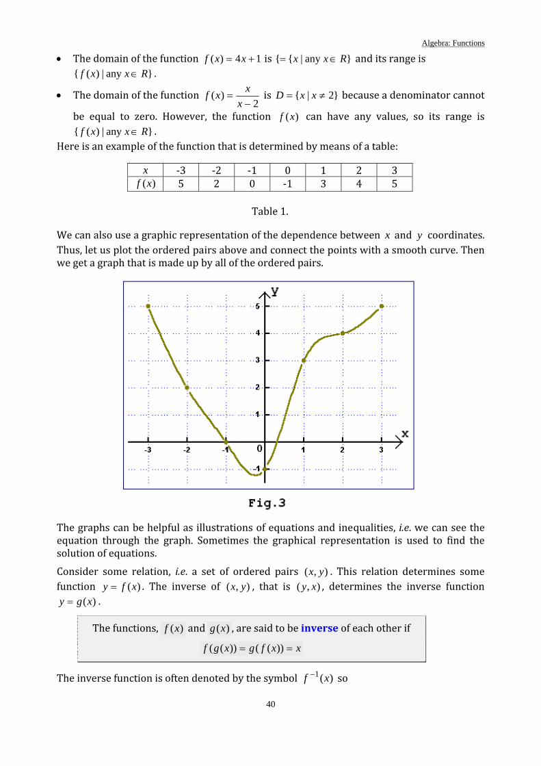
Here is an example of the function that is determined by means of a table:
x ‐3 ‐2 ‐1 0 1 2 3 )(xf 5 2 0 ‐1 3 4 5
Table 1.
We can also use a graphic representation of the dependence between x and y coordinates. Thus, let us plot the ordered pairs above and connect the points with a smooth curve. Then we get a graph that is made up by all of the ordered pairs.
The graphs can be helpful as illustrations of equations and inequalities, i.e. we can see the equation through the graph. Sometimes the graphical representation is used to find the solution of equations. Consider some relation, i.e. a set of ordered pairs ),( yx . This relation determines some function )(xfy = . The inverse of ),( yx , that is ),( xy , determines the inverse function
)(xgy = .
The functions, )(xf and )(xg , are said to be inverse of each other if
xxfgxgf == ))(())((
The inverse function is often denoted by the symbol )(1 xf − so

Algebra: Functions
41
xxffxff == −− ))(())(( 11 (1)
In order to find the inverse function of )(xf we have to replace )(xf with y , next replace x with y and y with x , and then solve the equality for y . Example: Find inverse functions of 27)( −= xxf . • 27)( −= xxf ⇒ 27 −= xy ⇒ 27 −= yx ⇒ 7)2( += xy
Thus, 7)2()(1 +=− xxf . Let us check whether this function is inverse of )(xf :
xxxxfxff =−+=−+
=+
=− 2)2(27
27)7
2())(( 1
xxxfxff =+−
==−= −−
72)27()27())(( 11 .
The inverse function test is correct.
4.3. Graphs of Some Algebraic Functions
1. Linear function in the slope‐intercept form: bkxxf +=)( . Slope of a line between two different points, ),( 11 yx and ),( 22 yx , is
12
12
xxyyk
−−
= .
It does not matter which two points are selected on a line; the slope is always the same. The slope of a horizontal line is equal to zero because in this case 21 yy = The slope of a vertical line is undefined because in this case 21 xx = but one never divides by zero. The point where a line crosses or touches the x ‐axis or y ‐axis is called an intercept. In order to find the x ‐intercepts for the graph of a function )(xfy = we have to set
0=y and solve the equation 0)( =xf . The y ‐intercept is found from the expression )0(fy = .
The graphs of some linear functions are shown in the drawing below. We can see the line 4=y with a zero‐slope, the lines with positive and negative slopes, and the vertical line whose slope is undefined. The intercepts are also shown.
Algebra: Functions
42
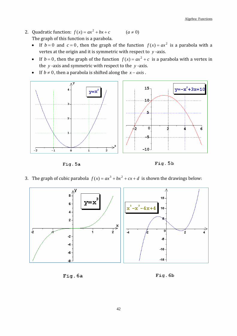
2. Quadratic function: cbxaxxf ++= 2)( )0( ≠a
The graph of this function is a parabola. • If 0=b and 0=c , then the graph of the function 2)( axxf = is a parabola with a
vertex at the origin and it is symmetric with respect to y ‐axis. • If 0=b , then the graph of the function caxxf += 2)( is a parabola with a vertex in
the y ‐axis and symmetric with respect to the y ‐axis. • If 0≠b , then a parabola is shifted along the axisx − .
3. The graph of cubic parabola dcxbxaxxf +++= 23)( is shown the drawings below:
Algebra: Functions
43
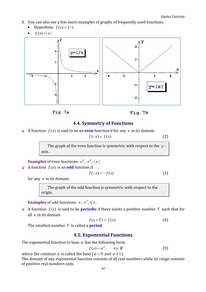
4. You can also see a few more examples of graphs of frequently used functions. • Hyperbola: xxf /1)( = • ||)( xxf =
4.4. Symmetry of Functions
A function )(xf is said to be an even function if for any x in its domain )()( xfxf =− (2)
The graph of the even function is symmetric with respect to the y ‐axis.
Examples of even functions: 2x , 4x , || x . A function )(xf is an odd function if
)()( xfxf −=− (3) for any x in its domain.
The graph of the odd function is symmetric with respect to the origin.
Examples of odd functions: x , 3x , x1 . A function )(xf is said to be periodic if there exists a positive number T such that for all x in its domain
)()( xfTxf =+ (4) The smallest number T is called a period.
4.5. Exponential Functions
The exponential function to base a has the following form: xaxf =)( , Rx∈ (5)
where the constant a is called the base ( 0>a and 1≠a ). The domain of any exponential function consists of all real numbers while its range consists of positive real numbers only.
Algebra: Functions
44
Here are some useful properties of exponential functions:
yx aa = if and only if yx = . If 1>a , then from yx < it follows that yx aa < . If 10 << a , then from yx < it follows that yx aa > .
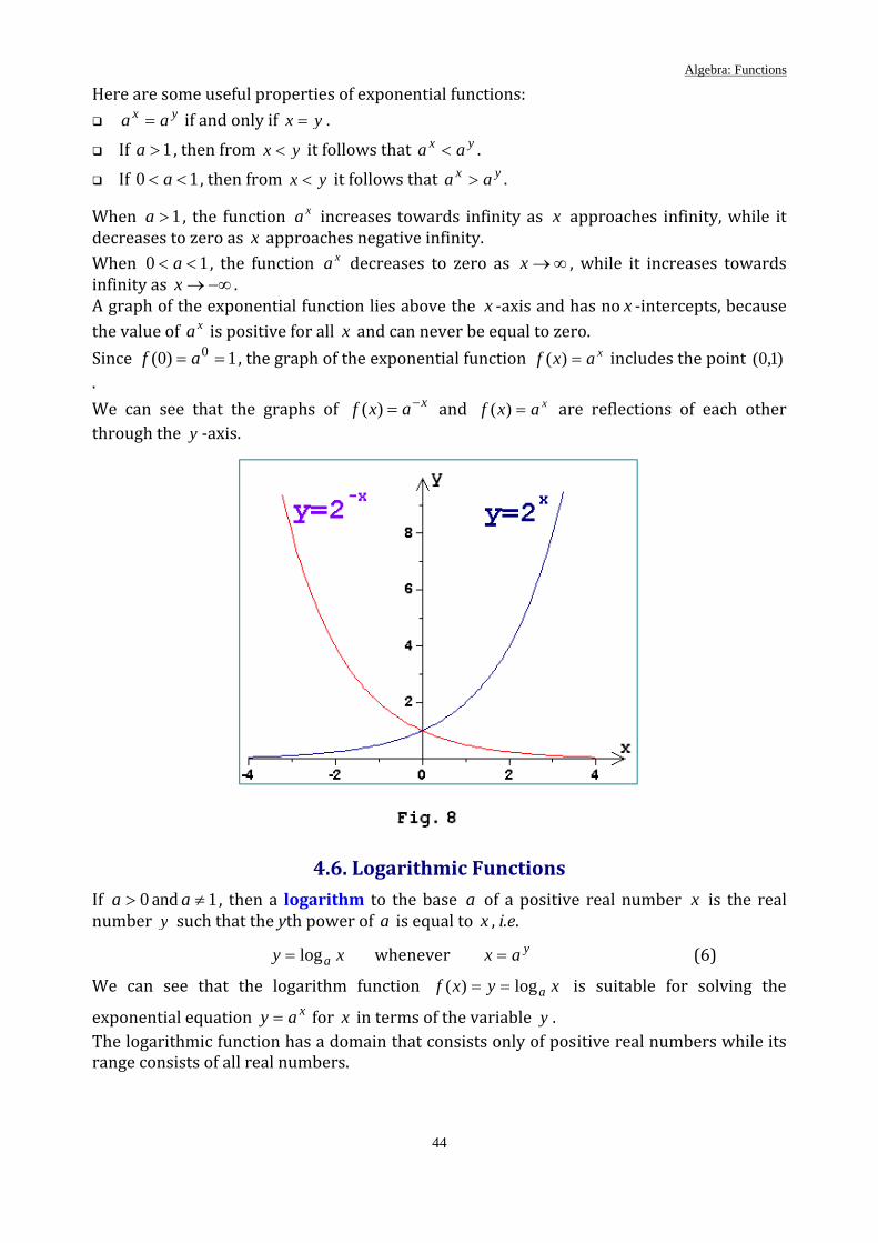
When 1>a , the function xa increases towards infinity as x approaches infinity, while it decreases to zero as x approaches negative infinity. When 10 << a , the function xa decreases to zero as ∞→x , while it increases towards infinity as −∞→x . A graph of the exponential function lies above the x ‐axis and has no x ‐intercepts, because the value of xa is positive for all x and can never be equal to zero. Since 1)0( 0 == af , the graph of the exponential function xaxf =)( includes the point )1,0(. We can see that the graphs of xaxf −=)( and xaxf =)( are reflections of each other through the y ‐axis.
4.6. Logarithmic Functions
If 1 and 0 ≠> aa , then a logarithm to the base a of a positive real number x is the real number y such that the yth power of a is equal to x , i.e.
xy alog= whenever yax = (6)
We can see that the logarithm function xyxf alog)( == is suitable for solving the
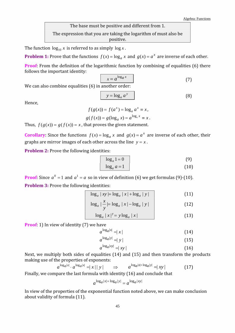
exponential equation xay = for x in terms of the variable y . The logarithmic function has a domain that consists only of positive real numbers while its range consists of all real numbers.
Algebra: Functions
45
The base must be positive and different from 1. The expression that you are taking the logarithm of must also be
positive.
The function x10log is referred to as simply xlog .
Problem 1: Prove that the functions xxf alog)( = and xaxg =)( are inverse of each other.
Proof: From the definition of the logarithmic function by combining of equalities (6) there follows the important identity:
xaax log= (7) We can also combine equalities (6) in another order:
ya ay log= (8)
Hence, xaafxgf x
ax ≡== log)())(( ,
xaxgxfg xa
a ≡== log)(log))(( . Thus, xxfgxgf == ))(())(( , that proves the given statement.
Corollary: Since the functions xxf alog)( = and xaxg =)( are inverse of each other, their graphs are mirror images of each other across the line xy = .
Problem 2: Prove the following identities:
01log =a (9) 1log =aa (10)
Proof: Since 10 =a and aa =1 so in view of definition (6) we get formulas (9)‐(10).
Problem 3: Prove the following identities:
||log||log||log yxxy aaa += (11)
||log||log||log yxyx
aaa −= (12)
||log||log xyx ay
a = (13)
Proof: 1) In view of identity (7) we have ||||log xa xa = (14)
||||log ya ya = (15)
||||log xya xya = (16) Next, we multiply both sides of equalities (14) and (15) and then transform the products making use of the properties of exponents:
||||||log||log yxaa xx aa =⋅ ⇒ ||||log||log xya yx aa =+ (17) Finally, we compare the last formula with identity (16) and conclude that
||log||log||log xyayaxa aa =+
In view of the properties of the exponential function noted above, we can make conclusion about validity of formula (11).

Algebra: Functions
46
2) Formula (12) can be proved in a similar way, but now we have to divide equalities (14) and (15) one by another. One can easily get the following relationship:
||||log||log
yxa yx aa =− (18)
Then, as above, we can write down the identity ||||log yxa yxa = and compare it with (18) to complete the proof. 3) In order to prove formula (13) we can make the following transformations:
yyxaxay xaa ||)( ||log||log ==⋅ yyxa xa ||||log =
yxaxay aa ||log||log =⋅ ⇒ ||log||log xyx ay
a = . Identity (13) is proved. When it is necessary to change in the base of a logarithmic function, the following equality can be used:
ax
xc
ca log
loglog = (19)
Corollary 1: By changing in the base of a logarithmic function we get a new identity:
xa
xax
ax
x aa
a
a
a
a
aa log
loglog
loglog
)1(loglog
log 11 −=−
===−
Therefore, a logarithmic function in the base a differs from a logarithmic function in the
base a1 in the sign only:
xx aa loglog1 −= (20)
Hence, their graphs are mirror images of each other across the x ‐axis.
Corollary 2: As above, making use of formulas (19), (13) and (10) we can also get a more general formula:
bx
abx
ax
x a
a
ab
a
aba
loglog
logloglog
log)(
−===
bx
x aba
loglog −= (16)
Examples:
• 3log5 =x ⇒ 12553 ==x
• 2log =x ⇒ 100102 ==x ⇒ 10000=x
• 42log42log16log 24
22 ===
• 16log)32(log3log2log 6666 ==⋅=+
• 543log
54)3(log
51)81(log81log 3
43
513
53 ====
• 25log2)4/20(log16log400log 52
555 ===−

Algebra: Functions
47
• 27log27log49log 72
77/1 1 −=−== −
4.6.1. Graphs of Logarithmic Functions
When 1>a , the function xy alog= increases towards infinity as ∞→x , while it will approach the y ‐axis asymptotically as 0→x . When 10 << a , the function xy alog= decreases continuously as x grows. Since 01log =a , the graph of each logarithmic function xxf alog)( = includes the point
)0,1( . The graphs of xxf alog)( = and xxf a/1log)( = are reflections of each other through the x ‐axis.
The below drawings illustrate the general property of inverse functions: the graphs of functions inverse of each other, xy alog= and xay = , are mirror images of each other across the line xy = .
Algebra: Functions
48
4.6.2. Natural Logarithm
One of the most important numbers used as the base for exponential and logarithmic functions is denoted as e . It is an irrational number, with its value approximated as
02874590452353671828182842.e = . Exponential and logarithmic functions with the base e occur in many practical applications, including those involving growth and decay. The natural logarithm of a positive real number x is defined as the logarithm to the base e of the number x . The natural logarithm xelog is denoted as xln :
xx elogln ≡ .
By definition, the equality yx =ln implies that xe y = . In order to convert logarithm from base 10 to base e , one can proceed from on formula (14):
xxxxxx
e
e ln43.03.2
ln10ln
ln10log
logloglog 10 ≈≈==≡
Since the functions xexf =)( and xxf ln)( = are inverse of each other, then
xex =ln
xe x =ln
The natural logarithm possesses the same properties as common logarithms. For instance, 1ln =e , 01ln = ..
Examples:
• 51ln
51)ln(ln 515 === eee
• 3ln213lnln
3ln −=−= ee
Algebra: Discrete Algebra
49
5. Discrete Algebra
5.1. Mathematical Induction Principle
Induction is a mathematical method suitable for proving an infinite sequence of statements. The statements can be represented, for example, by mathematical equations or inequalities involving the variable n. The main idea of this method is the following. Let nS be an infinite sequence of statements for ...,2,1,0=n If the statement nS is true for 0=n , and if the truth of nS implies that 1+nS is true, then nS is true for every non‐negative integer n .
The induction principle is based on a quite clear self‐intuitive premise. Indeed, if a particular statement nS is true for 0=n and nS implies that 1+nS is also true, then the statement nS is true for 110 =+=n . Similarly, nS is true for 211 =+=n , 312 =+=n , and so on for all non‐negative integers.
The mathematical induction principle includes three components: • the induction basis, • the induction hypothesis, • the induction step.
The induction basis is such a statement that being true gives a starting point for the induction. Therefore, in order to form the induction basis one has to prove (or check) that the statement nS is true for some integer kn = . Usually, one takes 0=k or 1=k . When we try to prove the truth of some general statement, it is quite naturally to check whether it is valid in a particular case.
The induction hypothesis is an assumption of the truth of the statement nS for some integer kn ≥ . In other words, we are ready to believe that the statement nS holds true for some integer kn ≥ . At this stage of induction we suppose the truth of the statement nS but prove nothing.
The induction step is the main stage of induction. If the statement nS implies 1+nS , provided kn ≥ , then nS must be true for all integers kn ≥ . Here, we proceed from verifications and assumptions to direct proving of the statement. So that in order to conclude that nS is true for any integer kn ≥ , we must prove the statement 1+nS being based on the assumption nS .
The above discussion shows that the mathematical induction method can be represented by the following pattern.
• The induction basis: The statement kS is true for some integer k . • The induction hypothesis: The statement nS holds true for some integer
kn ≥ . • The induction step: If the statement nS implies 1+nS , provided kn ≥ , then
nS must be true for all integers kn ≥ .

Algebra: Discrete Algebra
50
According to this scheme, the procedure of proving the validity of some statement nS for all integers kn ≥ also includes three stages: First, we need to originate a basis of induction. Second, we have to formulate an induction hypothesis. Finally, we must prove that the statement nS implies 1+nS that in view of a man‐made assumption allows to complete the proof.
Note: If nS ⇒ 1+nS but the statement kS is false, then we can at least conclude that nS is false for every kn ≤ , but we cannot say anything about nS for kn > .
The method of mathematical induction is very helpful in proving many statements about integers. The following examples illustrate the technique of it using in practice.
Example 1: Prove that nn >2 for all positive integers n . Proof: Let nS be the statement: nn >2 . Induction basis: The statement 1S is true: 1221 >= . Induction hypothesis: Suppose that the statement nS (i.e. inequality nn >2 ) holds for some integer 1≥n . Induction step: 12222 1 +≥+=⋅>⋅=+ nnnnnn . We can see that the inequality nn >2 implies the inequality )1(2 1 +>+ nn . Therefore, the proof of the above inequality by mathematical induction is complete.
Example 2: For all positive integers n we have the following formula:
2)1(
1
+=∑
=
nnin
i (1)
Note: The last formula is written using the Σ‐notation: nin
i+++=∑
=
...211
. We will employ
similar notations hereinafter. Proof: Let nS be statement (1).
Induction basis: The statement 1S is certainly true because 2211 ⋅
= .
Induction hypothesis: Let equality (1) hold true for some integer 1≥n .
Induction step: We verify the statement 1+nS which can be read as: 2
)2)(1(1
1
++=∑
+
=
nnin
i
.
If nS is true, then
2)2)(1()1
2)(1(
)hypothesisinduction (by )1(2
)1(
)1(1
1
1
++=++=
+++
=
++= ∑∑=
+
=
nnnn
nnn
niin
i
n
i
That is true. Therefore, nS is true for 1≥n by induction.
Algebra: Discrete Algebra
51
Example 3: For all positive integers n the following formula is valid:
2
1)12( ni
n
i=−∑
= (2)
Proof: Let nS be statement (2).
Induction basis: The statement 1S is read as: 11)12(1
1
=≡−∑=i
i . That is true.
Induction hypothesis: Suppose that equality (2) holds true for some integer 1≥n . Induction step: We verify that nS ⇒ 1+nS
2
21
1
1
)1()hypothesisinduction by ()12(
)1)1(2()12()12(
+=
++=
−++−=− ∑∑=
+
=
nnn
niin
i
n
i
If nS is true, then 1+nS must be true. Formula (2) is proved by induction.
Example 4: For all positive integers n we have the following formula:
6)12)(1(
1
2 ++=∑
=
nnnin
i (3)
Proof: Let nS be statement (3).
Induction basis: The statement 1S is read as: 16
)12)(11(112 =++
= . That is true.
Induction hypothesis: Let equality (3) be valid for some integer 1≥n .
Induction step: The statement 1+nS is read as: 6
)32)(2)(1(1
1
2 +++=∑
+
=
nnnin
i
.
We verify that nS ⇒ 1+nS
6)32)(2)(1(
))2(3)2(2(6
1
terms)groupingby ())63()42((6
1
)672(6
1
out) taken is rm(common te))1(6)12((6
1
)hypothesisinduction by ()1(6
)12)(1(
)1(
2
2
2
2
1
21
1
2
+++=
++++
=
++++
=
+++
=
++++
=
++++
=
++= ∑∑=
+
=
nnn
nnnn
nnnn
nnn
nnnn
nnnn
niin
i
n
i
Thus if nS is true, so is 1+nS .
Algebra: Discrete Algebra
52
Example 5: Use mathematical induction to prove that 2
1
3
2)1(⎟⎠⎞
⎜⎝⎛ +
=∑=
nnin
i (4)
is true for all positive integers n . Proof: Let nS be statement (4).
We check 1S which is read as: 12
)2(112
3 =⎟⎠⎞
⎜⎝⎛= . That is true.
Assume that equality (4) is true. Then
22
22
22
22
32
3
1
3
1
3
2)1)1)((1(
2)2)(1(
factoring)(by )2(4
)1(
)44(4
)1(
out) taken is mcommon ter())1(4(4
)1(
)hypothesisinduction by ()1(2
)1(
)1(
⎟⎠⎞
⎜⎝⎛ +++
=⎟⎠⎞
⎜⎝⎛ ++
=
++
=
+++
=
+++
=
++⎟⎠⎞
⎜⎝⎛ +
=
++= ∑∑==
nnnn
nn
nnn
nnn
nnn
niin
i
n
i
Thus if nS is true, so is 1+nS . Therefore, nS is true for all positive n by induction. Note: We can write down one more surprising formula by comparing formulas (1) and (4) with each other:
3332 ...21)...21( nn +++=+++ (5a)
That looks in the Σ‐notation as follows:
∑∑==
=⎟⎟⎠
⎞⎜⎜⎝
⎛ n
i
n
iii
1
32
1 (5b)
Example 6: Let n be any non‐negative integer and 1≠q , then the following formula is valid:
111
0 −−
=+
=∑ q
qqnn
i
i (6)
Proof: Let nS be statement (6). Let us check the above formula for 0=n : )1()1(10 −−== qqq The statement 0S is true. Suppose nS is true. Then we get

Algebra: Discrete Algebra
53
11
11
1)1(11
1
1)1(2
11
11
1
0
1
0
−−
=−−
=
−−+−
=
+−−
=+=
+++
++
++
+
=
+
=∑∑
qqqq
qqqq
nn
nn
nn
nn
i
in
i
i
by expanding the parentheses and combining similar terms. Thus, the statement nS implies 1+nS . Therefore, by the induction principle we can conclude that nS is true for all integers 0≥n . Formula (6) is proved.
Example 7: For all positive integers n the following formula is valid:
3)14()12(
2
1
2 −=−∑
=
nnin
i (7)
Proof: Let nS be statement (7).
Let us check 1S : 3
)14(11 −⋅= . That is true.
Let us denote that )12)(12()14( 2 +−=− nnn . Then the statement 1+nS is read as:
3)32)(12)(1(
3)1)1(2)(1)1(2)(1()12(
1
1
2
+++=
++−++=−∑
+
=
nnn
nnnin
i
Suppose that nS is true. Then we pass to the induction step:
3)1)(32)(12())1(3)1(2(
3)12(
))33()22((3
)12()352(3
)12(
))12(3)12((3
)12(
)12(3
)12)(12()12(3
)14(
)1)1(2()12()12(
22
222
2
1
21
1
2
+++=+++
+=
++++
=+++
=
++−+
=
+++−
=++−
=
−++−=− ∑∑=
+
=
nnnnnnn
nnnnnnn
nnnn
nnnnnnn
niin
i
n
i
We can see that nS implies 1+nS . Therefore, by induction principle we come to the conclusion that nS is true for all positive integers n .
Example 8: Use mathematical induction to check the validity of the assumption 22 nn > (8)
for positive integers n .
Solution: Let nS be statement (8). Let us check 1S : 12 > . That is true.
Algebra: Discrete Algebra
54
Suppose that nS is true. Then 21 2222 nnn >⋅=+ .
So we must test whether 22 )1(2 +> nn . 22 )1(2 +> nn ⇒ 0122 >−− nn ⇒ 21+>n ⇒ 3≥n .
Therefore, the statement 1S cannot be taken as the induction basis. Let us check nS for 3≥n :
3=n : 9382 23 =>= . That is a false statement. 4=n : 164162 24 =>= . That is false. 5=n : 255322 25 =>= . That is true.
Thus, the starting point is 5=n . We can see that the statement 5S is true and nS implies 1+nS for all integers 5≥n . Hence, 22 nn > for all integers 5≥n .
5.2. Arithmetic Progression
An arithmetic progression is a sequence in which each term (after the first) is determined by adding a constant to the preceding term. This constant is said to be the common difference of the arithmetic progression. The following equations express this sentence mathematically:
daa nn +=+1 (9) ndaan +=+ 11 (10)
Here 1a is the first term of the arithmetic progression; na is its nth term;
d is the common difference of the arithmetic progression; Nn∈ .
Consider the sum of the first n terms of an arithmetic progression:
nn
n
kkn aaaaaS ++++== −
=∑ 121
1... (11)
Let us note that sum (11) consists of equal pairs:
...)()(
)()(
2312
1211
=+=−++=
+=−++=+
−−
−
nn
nnn
aadadaaadadaaa
Therefore, the sum nS holds its value if each term in (11) is replaced by 2)( 1 naa + . Since sum (11) contains n terms, so we get the following formula:
2)( 1
1
naaaS n
n
kkn
+==∑
= (12)
The last formula can be also written as
ndnaSn )2
)1(( 1−
+= (13)
making use of the equality dnaan )1(1 −+= .

Algebra: Discrete Algebra
55
Example: Calculate the sum of the first 10 terms of the arithmetic progression if 42 =a and 225 =a .
Solution: From equality (2) it follows that 412 =+= daa (14) 22415 =+= daa (15)
We can find the common difference of the arithmetic progression by subtracting equality (14) from (15):
183 =d ⇒ 6=d . Then from (14) we calculate the first term of the arithmetic progression:
26441 −=−=−= da The sum of the first 10 terms of the arithmetic progression in view of formula (13) is
25010)2
692(10 =⋅⋅
+−=S
5.3. Geometric Progression
A geometric progression is a sequence in which each term (after the first) is determined by multiplying the preceding term by a constant. This constant is called the common ratio of the arithmetic progression. The following equations express this statement mathematically:
qaa nn =+1 (16) n
n qaa 11 =+ (17)
Here 1a is the first term of the geometric progression; na is the nth term of the geometric progression;
q is the common ratio of the geometric progression; Nn∈ .
Let us calculate the sum of the first n terms of the geometric progression:
.)...1(
......1
11
121
11
2111321
∑−
=
−
−
=++++=
++++=++++=n
k
kn
nnn
qaqqqa
qaqaqaaaaaaS (18)
At fist, let us multiply both sides of the above equality by the factor q :
∑=
=n
k
kn qaqS
21 , (19)
then subtract equality (18) from equality (19) and simplify both sides:
∑∑−
==
−=−1
11
21
n
k
kn
k
knn qaqaSqS ⇒
)()()1(1
21
1
21 qqaqqaqS
n
k
kn
k
nkn +−+=− ∑∑
−
=
−
=
⇒
)1()1( 1 −=− nn qaqS
The sum nS can be obtained by dividing both sides of the latter by the factor )1( −q , if 1≠q:
Algebra: Discrete Algebra
56
1)1(1
−−
=qqa
Sn
n (20)
Note: If 1|| <q , then 0→nq when ∞→n . Hence, the sum of an infinite number of terms of decreasing geometric progression is equal to
qaS−
=∞ 11 (21)
Example: Calculate the sum of the first ten terms of the geometric progression and find the seventh term if the sum of the first five terms 315 =S and the common ratio 2=q . Solution:
1) From formula (20) we get 1132
311
)1(5
51 =
−=
−−
=q
qSa .
2) Making use of formula (20) for 10=n we get 1023121010 =−=S .
3) From formula (17) we get 6426617 === qaa .
5.4. Binomial Theorem
At first let us introduce binomial coefficients defined by the following formula:
)!(!!
knknC k
n −= (22)
The symbol “ !n ” has to be read as “n factorial” and means the product of all natural numbers from 1 to n :
nn ⋅⋅⋅= ...21!
A zero factorial is equal to one unit by definition: 1!0 = . It is clear that !)1()!1( nnn ⋅+=+
The binomial coefficient knC gives a number of ways for choosing k objects from a set of n
objects, regardless of the order in which the k objects are chosen. Making use of definition (22) we get the following relationships:
)!(!!
knknCC k
nkn
n −==−
1)!0(!0
!0 =−
==nnCC n
nn
nnnCn =−
=)!1(!1
!1
One can also check the validity of the recursion relation between the binomial coefficients kn
kn
kn CCC 1
1+
− =+ (23)
which allows by means of constructing the Pascal’s triangle to evaluate knC in a simple way.

Algebra: Discrete Algebra
57
Pascal's triangle is a triangular array of binomial coefficients. Its structure is evident from the table below.
00C 1 k=0
kC1 1 1 k=0, 1
kC2 1 2 1 k=0, 1, 2
kC3 1 3 3 1 k=0, 1, 2, 3
kC4 1 4 6 4 1 k=0, 1,2,3,4
kC5 1 5 1
0 10
5 1 k=0, 1,2,3,4,5
… … … … … … …
Examples:
• 32112
02
13 =+=+= CCC
• 43113
03
14 =+=+= CCC
• 63323
13
24 =+=+= CCC
• 51444
34
45 =+=+= CCC
The Binomial Theorem: For any positive integer n and real a and b the following formula is valid:
kknn
k
kn
n baCba −
=∑=+
0)( . (24)
Setting 1=a and xb = we get from the last formula:
kn
k
kn
n xCx ∑=
=+0
)1(
One can see that binomial coefficients are the coefficients of x in the expansion of nx)1( + . Examples:
• 22222
12
202
2 2)( bababCabCaCba ++=++=+ .
• 3223333
223
213
303
3 33)( babbaabCbaCbaCaCba +++=+++=+
• 543223455 510105)( babbababaaba +++++=+
The binomial theorem is employed in calculus, combinatorial analysis, statistics, etc.
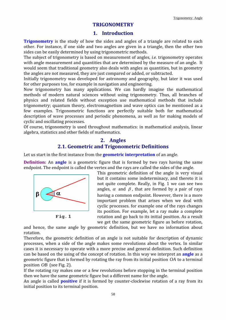
Trigonometry: Angle
58
TRIGONOMETRY
1. Introduction
Trigonometry is the study of how the sides and angles of a triangle are related to each other. For instance, if one side and two angles are given in a triangle, then the other two sides can be easily determined by using trigonometric methods. The subject of trigonometry is based on measurement of angles, i.e. trigonometry operates with angle measurement and quantities that are determined by the measure of an angle. It would seem that traditional geometry also deals with angles as quantities, but in geometry the angles are not measured, they are just compared or added, or subtracted. Initially trigonometry was developed for astronomy and geography, but later it was used for other purposes too, for example in navigation and engineering. Now trigonometry has many applications. We can hardly imagine the mathematical methods of modern natural sciences without using trigonometry. Thus, all branches of physics and related fields without exception use mathematical methods that include trigonometry; quantum theory, electromagnetism and wave optics can be mentioned as a few examples. Trigonometric functions are perfectly suitable both for mathematical description of wave processes and periodic phenomena, as well as for making models of cyclic and oscillating processes. Of course, trigonometry is used throughout mathematics: in mathematical analysis, linear algebra, statistics and other fields of mathematics.
2. Angles 2.1. Geometric and Trigonometric Definitions
Let us start in the first instance from the geometric interpretation of an angle. Definition: An angle is a geometric figure that is formed by two rays having the same endpoint. The endpoint is called the vertex and the rays are called the sides of the angle.
This geometric definition of the angle is very visual but it contains some indeterminacy, and thereto it is not quite complete. Really, in Fig. 1 we can see two angles, α and β , that are formed by a pair of rays having a common endpoint. However, there is a more important problem that arises when we deal with cyclic processes. for example one of the rays changes its position. For example, let a ray make a complete rotation and go back to its initial position. As a result we get the same geometric figure as before rotation,
and hence, the same angle by geometric definition, but we have no information about rotation. Therefore, the geometric definition of an angle is not suitable for description of dynamic processes, when a side of the angle makes some revolutions about the vertex. In similar cases it is necessary to operate with a more precise and general definition. Such definition can be based on the using of the concept of rotation. In this way we interpret an angle as a geometric figure that is formed by rotating the ray from its initial position OA to a terminal position OB (see Fig. 2). If the rotating ray makes one or a few revolutions before stopping in the terminal position then we have the same geometric figure but a different name for the angle. An angle is called positive if it is formed by counter‐clockwise rotation of a ray from its initial position to its terminal position.
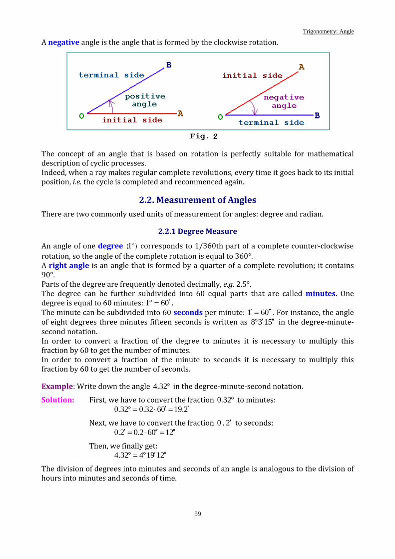
Trigonometry: Angle
59
A negative angle is the angle that is formed by the clockwise rotation.
The concept of an angle that is based on rotation is perfectly suitable for mathematical description of cyclic processes. Indeed, when a ray makes regular complete revolutions, every time it goes back to its initial position, i.e. the cycle is completed and recommenced again.
2.2. Measurement of Angles
There are two commonly used units of measurement for angles: degree and radian.
2.2.1 Degree Measure
An angle of one degree )( o1 corresponds to 1/360th part of a complete counter‐clockwise rotation, so the angle of the complete rotation is equal to 360°. A right angle is an angle that is formed by a quarter of a complete revolution; it contains 90°. Parts of the degree are frequently denoted decimally, e.g. 2.5°. The degree can be further subdivided into 60 equal parts that are called minutes. One degree is equal to 60 minutes: 061 ′=° . The minute can be subdivided into 60 seconds per minute: 061 ′′=′ . For instance, the angle of eight degrees three minutes fifteen seconds is written as 5138 ′′′° in the degree‐minute‐second notation. In order to convert a fraction of the degree to minutes it is necessary to multiply this fraction by 60 to get the number of minutes. In order to convert a fraction of the minute to seconds it is necessary to multiply this fraction by 60 to get the number of seconds.
Example: Write down the angle °32.4 in the degree‐minute‐second notation.
Solution: First, we have to convert the fraction °32.0 to minutes: 2.190632.032.0 ′=′⋅=°
Next, we have to convert the fraction 20 ′. to seconds: 21062.02.0 ′′=′′⋅=′
Then, we finally get: 2191432.4 ′′′°=°
The division of degrees into minutes and seconds of an angle is analogous to the division of hours into minutes and seconds of time.
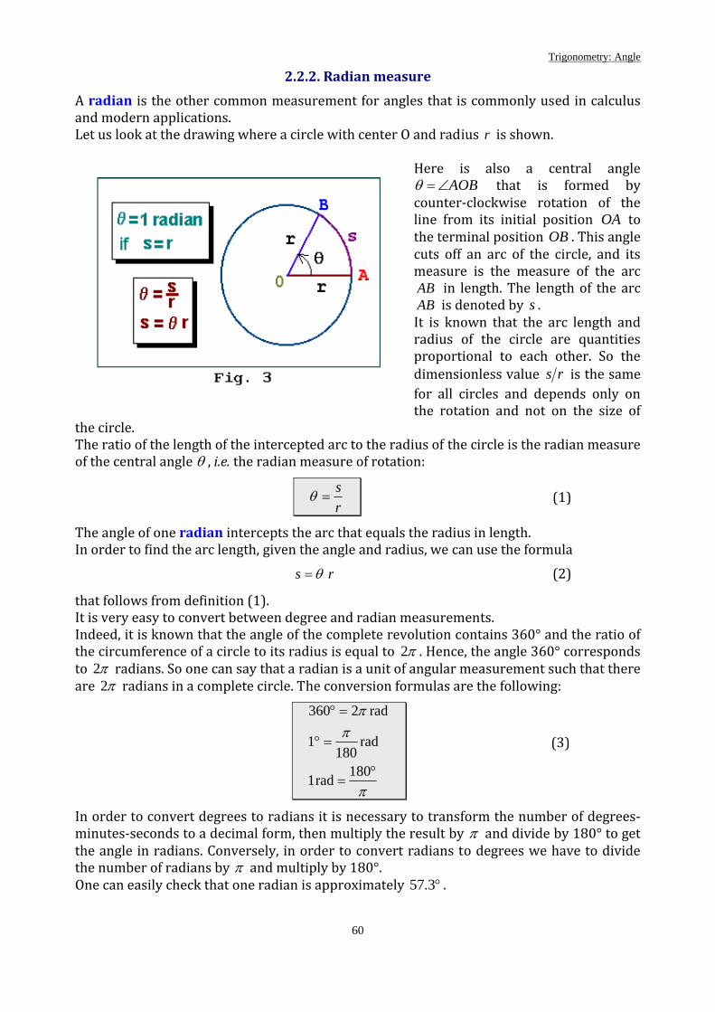
Trigonometry: Angle
60
2.2.2. Radian measure
A radian is the other common measurement for angles that is commonly used in calculus and modern applications. Let us look at the drawing where a circle with center O and radius r is shown.
Here is also a central angle AOB∠=θ that is formed by
counter‐clockwise rotation of the line from its initial position OA to the terminal position OB . This angle cuts off an arc of the circle, and its measure is the measure of the arc AB in length. The length of the arc AB is denoted by s . It is known that the arc length and radius of the circle are quantities proportional to each other. So the dimensionless value rs is the same for all circles and depends only on the rotation and not on the size of
the circle. The ratio of the length of the intercepted arc to the radius of the circle is the radian measure of the central angle θ , i.e. the radian measure of rotation:
rs
=θ (1)
The angle of one radian intercepts the arc that equals the radius in length. In order to find the arc length, given the angle and radius, we can use the formula
rs θ= (2)
that follows from definition (1). It is very easy to convert between degree and radian measurements. Indeed, it is known that the angle of the complete revolution contains 360° and the ratio of the circumference of a circle to its radius is equal to π2 . Hence, the angle 360° corresponds to π2 radians. So one can say that a radian is a unit of angular measurement such that there are π2 radians in a complete circle. The conversion formulas are the following:
π
ππ
°=
=°
=°
180rad1
rad180
1
rad2360
(3)
In order to convert degrees to radians it is necessary to transform the number of degrees‐minutes‐seconds to a decimal form, then multiply the result by π and divide by 180° to get the angle in radians. Conversely, in order to convert radians to degrees we have to divide the number of radians by π and multiply by 180°. One can easily check that one radian is approximately °3.57 .
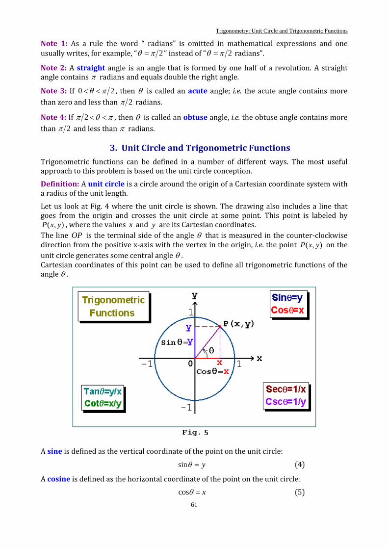
Trigonometry: Unit Circle and Trigonometric Functions
61
Note 1: As a rule the word “ radians” is omitted in mathematical expressions and one usually writes, for example, “ 2πθ = ” instead of “ 2πθ = radians”.
Note 2: A straight angle is an angle that is formed by one half of a revolution. A straight angle contains π radians and equals double the right angle.
Note 3: If 20 πθ << , then θ is called an acute angle; i.e. the acute angle contains more than zero and less than 2π radians.
Note 4: If πθπ <<2 , then θ is called an obtuse angle, i.e. the obtuse angle contains more than 2π and less than π radians.
3. Unit Circle and Trigonometric Functions Trigonometric functions can be defined in a number of different ways. The most useful approach to this problem is based on the unit circle conception. Definition: A unit circle is a circle around the origin of a Cartesian coordinate system with a radius of the unit length. Let us look at Fig. 4 where the unit circle is shown. The drawing also includes a line that goes from the origin and crosses the unit circle at some point. This point is labeled by
),( yxP , where the values x and y are its Cartesian coordinates. The line OP is the terminal side of the angle θ that is measured in the counter‐clockwise direction from the positive x‐axis with the vertex in the origin, i.e. the point ),( yxP on the unit circle generates some central angle θ . Cartesian coordinates of this point can be used to define all trigonometric functions of the angle θ .
A sine is defined as the vertical coordinate of the point on the unit circle:
y=θsin (4)
A cosine is defined as the horizontal coordinate of the point on the unit circle: x=θcos (5)
Trigonometry: Unit Circle and Trigonometric Functions
62
Both functions, tangent and cotangent, are defined as the ratio of Cartesian coordinates:
xy
=θtan if 0≠x (6a)
yx
=θcot if 0≠y (7a)
It is clear that θtan and θcot can be also expressed in terms of θsin and θcos using the above definitions:
θθθ
cossintan = (6b)
θθθ
sincoscot = (7b)
We see that the tangent is reciprocal of the cotangent and vice versa:
θθ
θθ
tan1cot
cot1tan
=
= (8)
A reciprocal of a cosine is known as a secant:
x1
cos1sec ==θ
θ if 0≠x (9)
A cosecant is defined as a reciprocal of a sine:
y1
sin1csc ==θ
θ if 0≠y (10)
Thereby all trigonometric functions are related to each other trough simple identities. We can denote that the sine and cosine together are the “primary” trigonometric functions, whereas the others are “secondary”, i.e. they can be defined in terms of sine and cosine. Summary: In order to find trigonometric functions of a given angle θ we can draw a line from the origin at the angle θ to get the point where this line crosses the unit circle. Then the x ‐coordinate of this point gives θcos and its y ‐coordinate is θsin . All the other trigonometric functions can be found by using θsin and θcos .
Example 1: Calculate θsin and θcos of the angles nπθ = , where In∈ .
Solution: The angles ...,4,2,0 ππθ ±±= correspond to the point )0,1( on the unit circle, while the angles ...,5,3, πππθ ±±±= correspond to the point )0,1(− . The y ‐coordinate is equal to zero in both cases and therefore,
0sin =nπ , In∈ (11)
However, 1cos =nπ for even numbers n , and 1cos −=nπ for odd numbers n . Both odd‐even cases can be combined into uniform identity:
nn )1(cos −=π , In∈ (12)
Trigonometry: Basic Properties of Trigonometric Functions
63
3.1. Domains of the Trigonometric Functions Some trigonometric functions, the sine and cosine namely, are defined for any θ , but the others are not defined for certain angles. Therefore, we have to determine their domains.
• Both functions, the tangent and secant, are defined if and only if 0≠x , because a denominator cannot be equal to zero. Any point with a zero‐ x ‐coordinate lies on the −y axis, so the condition 0≠x implies
nππθ +≠2
, In∈ .
• The cotangent and cosecant are defined if and only if 0≠y . Any point with a zero‐ y ‐coordinate lies on the x ‐ axis, and the condition 0≠y implies
nπθ ≠ , In∈ .
In summary, the above can be represented by the following table:
Trigonometric function
Domain
θsin θcos
any R∈θ
θtan θsec
nππθ +≠ 2 , In∈
θcot θcsc
nπθ ≠ , In∈
Table 1
4. Basic Properties of Trigonometric Functions
Here are the most important properties of trigonometric functions. We start out from the properties that can be easily derived using the definitions of trigonometric functions. Let us go back to the unit circle.
4.1. The Fundamental Trigonometric Identity Let ),( yx be any point on the unit circle, i.e. its distance to the origin is equal to one unit.
The square of this distance 21 is equal to the sum of squares of coordinates by the Pythagorean Theorem:
122 =+ yx In view of definitions (4) and (5) we get the fundamental trigonometric identity:
1cossin 22 =+ θθ (13)
Corollary. For any θ the following inequalities are valid: 1|sin| ≤θ 1|cos| ≤θ
Problem 1: Prove the following formula:
θθ 2
2
cos1tan1 =+ (14)
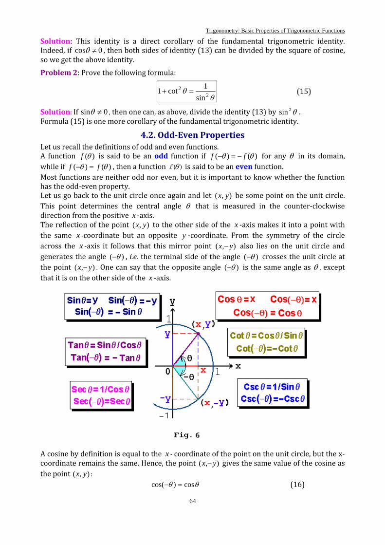
Trigonometry: Basic Properties of Trigonometric Functions
64
Solution: This identity is a direct corollary of the fundamental trigonometric identity. Indeed, if 0cos ≠θ , then both sides of identity (13) can be divided by the square of cosine, so we get the above identity. Problem 2: Prove the following formula:
θθ 2
2
sin1cot1 =+ (15)
Solution: If 0sin ≠θ , then one can, as above, divide the identity (13) by θ2sin . Formula (15) is one more corollary of the fundamental trigonometric identity.
4.2. OddEven Properties Let us recall the definitions of odd and even functions. A function )(θf is said to be an odd function if )()( θθ ff −=− for any θ in its domain, while if )()( θθ ff =− , then a function )(θf is said to be an even function. Most functions are neither odd nor even, but it is important to know whether the function has the odd‐even property. Let us go back to the unit circle once again and let ),( yx be some point on the unit circle. This point determines the central angle θ that is measured in the counter‐clockwise direction from the positive x ‐axis. The reflection of the point ),( yx to the other side of the x ‐axis makes it into a point with the same x ‐coordinate but an opposite y ‐coordinate. From the symmetry of the circle across the x ‐axis it follows that this mirror point ),( yx − also lies on the unit circle and generates the angle )( θ− , i.e. the terminal side of the angle )( θ− crosses the unit circle at the point ),( yx − . One can say that the opposite angle )( θ− is the same angle as θ , except that it is on the other side of the x ‐axis.
A cosine by definition is equal to the x ‐ coordinate of the point on the unit circle, but the x‐coordinate remains the same. Hence, the point ),( yx − gives the same value of the cosine as the point ),( yx :
θθ cos)cos( =− (16)
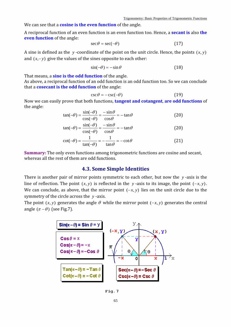
Trigonometry: Basic Properties of Trigonometric Functions
65
We can see that a cosine is the even function of the angle. A reciprocal function of an even function is an even function too. Hence, a secant is also the even function of the angle:
)sec(sec θθ −= (17)
A sine is defined as the y ‐coordinate of the point on the unit circle. Hence, the points ),( yx and ),( yx − give the values of the sines opposite to each other:
θθ sin)sin( −=− (18)
That means, a sine is the odd function of the angle. As above, a reciprocal function of an odd function is an odd function too. So we can conclude that a cosecant is the odd function of the angle:
)csc(csc θθ −−= (19) Now we can easily prove that both functions, tangent and cotangent, are odd functions of the angle:
θθθ
θθθ tan
cossin
)cos()sin()tan( −=
−=
−−
=− (20)
θθθ
θθθ tan
cossin
)cos()sin()tan( −=
−=
−−
=− (20)
θθθ
θ cottan
1)tan(
1)cot( −=−=−
=− (21)
Summary: The only even functions among trigonometric functions are cosine and secant, whereas all the rest of them are odd functions.
4.3. Some Simple Identities
There is another pair of mirror points symmetric to each other, but now the y ‐axis is the line of reflection. The point ),( yx is reflected in the y ‐axis to its image, the point ),( yx− . We can conclude, as above, that the mirror point ),( yx− lies on the unit circle due to the symmetry of the circle across the y ‐axis. The point ),( yx generates the angle θ while the mirror point ),( yx− generates the central angle )( θπ − (see Fig.7).
Trigonometry: Basic Properties of Trigonometric Functions
66
These points, ),( yx and ),( yx− , give values of the sines equal to each other but the opposite values of the cosines:
θθπθθπ
cos)cos(sin)sin(−=−
=− (22)
It follows from above that
θθπθθπθθπθθπ
csc)csc(sec)sec(
cot)cot(tan)tan(
−=−=−−=−−=−
(23)
Now let us consider the pair of points ),( yx and ),( yx −− . They both lie on the unit circle and are symmetric to each other relative to the origin. The point ),( yx corresponds to the angle θ while the point ),( yx −− generates the central angle )( θπ + . One can easy prove in a similar way the following identities:
θθπθθπθθπθθπ
cot)cot(tan)tan(
cos)cos(sin)sin(
=+=+−=+−=+
(24)
It is clear that similar identities are also valid for secant and cosecant.
4.4. Periodicity
Now let us suppose that the terminal side of the angle θ makes complete revolutions, i.e. rotates until it coincides with the position before. Then the angle of the entire rotation
)2( π± is added to the primary angle θ . The sign depends on the direction of rotation: minus is taken when the terminal side rotates in the clockwise direction. We can imagine any number of such rotations, and each of them adds the value )2( π± to the angle. That means the point ),( yxP on the unit circle generates the infinite set of angles,
nπθ 2+ ( In∈ ), such that each one taken separately corresponds, just as θ , to the same point ),( yxP . Therefore, we can conclude that for any θ the following identities are valid:
θπθθπθ
cos)2cos(sin)2sin(
=+=+
nn
(25)
We can see that the sine and cosine are periodic functions because for all θ there exists a positive number T such that θθ sin)sin( =+ T and θθ cos)cos( =+T . The value π2=T is the smallest positive value for which these equations are valid. Therefore, the functions
θsin and θcos have period π2 . The other trigonometric functions are also periodic because they are defined through the periodic functions cosine and sine. The periodic functions θsec and θcsc have the same period π2 :
θπθθπθ
csc)2csc(sec)2sec(
=+=+
nn
(26)
The periodic functions θtan and θcot have a different period that is equal to π as that follows from identities (24):
θπθθπθ
cot)cot(tan)tan(
=+=+
nn
(27)
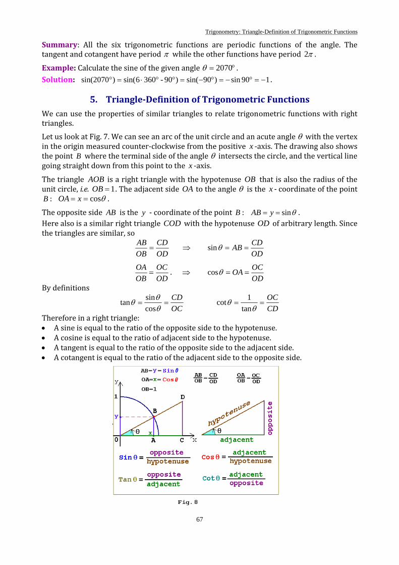
Trigonometry: Triangle-Definition of Trigonometric Functions
67
Summary: All the six trigonometric functions are periodic functions of the angle. The tangent and cotangent have period π while the other functions have period π2 .
Example: Calculate the sine of the given angle °= 2070θ . Solution: 190sin)90sin()90-3606sin()sin(2070 −=°−=°−=°°⋅=° .
5. TriangleDefinition of Trigonometric Functions
We can use the properties of similar triangles to relate trigonometric functions with right triangles. Let us look at Fig. 7. We can see an arc of the unit circle and an acute angle θ with the vertex in the origin measured counter‐clockwise from the positive x ‐axis. The drawing also shows the point B where the terminal side of the angle θ intersects the circle, and the vertical line going straight down from this point to the x ‐axis.
The triangle AOB is a right triangle with the hypotenuse OB that is also the radius of the unit circle, i.e. 1=OB . The adjacent side OA to the angle θ is the x ‐ coordinate of the point B : θcos== xOA .
The opposite side AB is the y ‐ coordinate of the point B : θsin== yAB . Here also is a similar right triangle COD with the hypotenuse OD of arbitrary length. Since the triangles are similar, so
ODCD
OBAB
= ⇒ ODCDAB ==θsin
ODOC
OBOA
= . ⇒ ODOCOA ==θcos
By definitions
OCCD
==θθθ
cossintan
CDOC
==θ
θtan
1cot
Therefore in a right triangle: • A sine is equal to the ratio of the opposite side to the hypotenuse. • A cosine is equal to the ratio of adjacent side to the hypotenuse. • A tangent is equal to the ratio of the opposite side to the adjacent side. • A cotangent is equal to the ratio of the adjacent side to the opposite side.

Trigonometry: Triangle-Definition of Trigonometric Functions
68
The last statements are known as right triangledefinition of trigonometric functions. Example: There are given sides 2=a and 5=b in the right triangle. Let a be the opposite side to the angle θ . Find the values of all trigonometric functions of the angle θ . Solution: Let us denote the hypotenuse of the triangle by c . 1) Find the hypotenuse using the Pythagorean Theorem:
2925422 =+=+= bac
2) Calculate trigonometric functions using the right triangle‐based definitions: 292sin == caθ 295cos == cbθ
52tan == baθ 25cot == abθ 529cos1sec == θθ 229sin1csc == θθ
Now let us look at Fig. 9 where a right triangle with a hypotenuse of an arbitrary length c is shown. The sides in the right triangle are denoted by a and b .
• The side a is adjacent to the angle θ , so ca=θcos by definition. The side a is also opposite to the angle ϕ , so ca=ϕsin . Hence,
ϕθ sincos = • In a similar way one can easily get that ϕθ cossin = . Since θπϕ −= 2 , so we see that
sine and cosine are complementary:
)2
cos(sin θπθ −= )2
sin(cos θπθ −= (28)
It is quite clear that the same statement is valid for another pair of functions, a tangent and a cotangent:
)2
cot(tan θπθ −= )2
tan(cot θπθ −= (29)
5.1. Sines and Cosines for Special Angles There are special reference angles that come up in many of the calculations: °30 , °45 and
°60 .
Problem 1: Find the values of trigonometric functions of the angles °30 and °60 . Solution: Let us look fist at Fig. 9 where the right triangle ABC with a hypotenuse AB is shown. There is also the right triangle ACD that is a mirror reflection of the triangle ABC relative to the side AB . So we have the equilateral triangle ABD . Let the hypotenuse AB be denoted by c .

Trigonometry: Triangle-Definition of Trigonometric Functions
69
It follows from the equilateral triangle ABD that cABBD == and 2cBC = .
1) 2160cos30sin ==°=°
ABBC
2) 22 )()( BCABAC −= by the Pythagorean Theorem. 3) Using the above equalities we get 23cAC = .
4) 2330cos60sin ==°=°
ABAC
5) 33
31
30cos30sin60cot30tan ==°°
=°=°
6) 360cos60sin30cot60tan =°°
=°=°
7) 3
323
230cos
160csc30sec ==°
=°=°
8) 260cos
130csc60sec =°
=°=°
Problem 2: Find the values of trigonometric functions of the angle °45 . Solution: Let us consider the isosceles right triangle that is shown in Fig. 11.
1) Both sides in the triangle are equal to each other and denoted by a . The hypotenuse is denoted by c ; it can be found by using the Pythagorean Theorem: 222 aaac =+= .
2) 222145cos45sin ===°=° ca .
3) 145cot45tan ==°=° aa .
4) 245sin145csc45sec =°=°=° .

Trigonometry: Addition Formulas for Sine and Cosine
70
The values of trigonometric functions of special angles in the radian and degree measurements are placed into the following table:
θ radian
θ degree
θsin θcos θtan θcot
0 0o 0 20 1 0 Undefined
6π 30o
21
21
23
33 3
4π 45o
22
22
22
1 1
3π 60o
23
23
21 3
33
2π 90o 1
24 0 Undefined 0
Table 2.
Note: The set of the sine data is represented by the two columns, where the second column
attracts your attention to the simple pattern of the quantities: 24,
23,
22,
21,
20
and prompts us a simple way to memorize the table above. Naturally, you can always go back to the usual form: 020 = , 2121 = and 124 = . The column that includes the cosine data set is inverse to that of the sine one.
6. Addition Formulas for Sine and Cosine
Look at the following drawing. There are two lines, OP and OQ , going from the origin. The line OQ is the terminal side of the angle α that is measured in the counter‐clockwise direction from the positive x ‐axis with the vertex in the origin. The line OP is the terminal side of the angle β that is measured in the counter‐clockwise direction from the line OQ with the vertex in the origin too. The point P is taken at a distance of the unit length from the origin, i.e. the point P lies on the imaginable unit circle. The point Q is taken to be the foot of the perpendicular that is dropped from the point P . Therefore, we get the right triangle OPQ with the hypotenuse 1=OP . We can also see perpendiculars that are dropped from the points P and Q onto the x ‐ and y ‐axes. In that way two similar right triangles are formed (see Fig. 12).
1) The x ‐ coordinate of the point P , viz. x , gives the cosine of the angle )( βα + , while the y ‐ coordinate of this point, that is y , is equal to the sine of the same angle:
x=+ )cos( βα y=+ )sin( βα
2) The coordinates of the point P can be represented as follows:
)()(
11
11
yyyyxxxx
−+=−−=
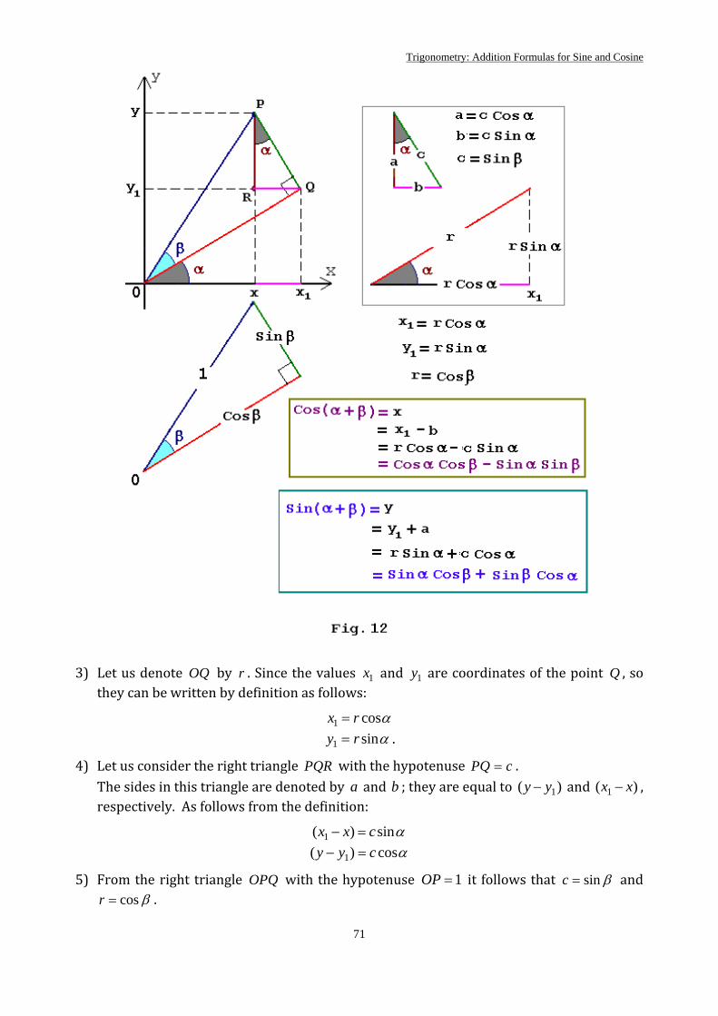
Trigonometry: Addition Formulas for Sine and Cosine
71
3) Let us denote OQ by r . Since the values 1x and 1y are coordinates of the point Q , so they can be written by definition as follows:
αcos1 rx = αsin1 ry = .
4) Let us consider the right triangle PQR with the hypotenuse cPQ = . The sides in this triangle are denoted by a and b ; they are equal to )( 1yy − and )( 1 xx − , respectively. As follows from the definition:
αsin)( 1 cxx =− αcos)( 1 cyy =−
5) From the right triangle OPQ with the hypotenuse 1=OP it follows that βsin=c and βcos=r .

Trigonometry: Addition Formulas for Sine and Cosine
72
6) Now we can substitute the expressions obtained into the above to get formulas of prime importance that are called addition formulas for sine and cosine:
αββαβα cossincossin)sin( +=+ (30)
βαβαβα sinsincoscos)cos( −=+ (31)
These worthwhile formulas are the most important trigonometric formulas in every respect. • They are valid for any values of α and β . • One can derive all trigonometric formulas and properties using addition formulas for
sine and cosine only. For instance, subtraction formulas for sine and cosine can be obtained from the above by substituting β for )( β− :
αββαβα cossincossin)sin( −=− (32)
βαβαβα sinsincoscos)cos( +=− (33)
Finally, we can combine addition formulas and subtraction formulas into one pair of addition and subtraction formulas for sine and cosine:
αββαβα cossincossin)sin( ±=± (34)
βαβαβα sinsincoscos)cos( m=± (35)
Advice: Try to get into the habit of checking whether the given formula is correct. • Attempt to reproduce the already known results by fitting a suitable proportion
between variables. • Analyze and investigate special or singular cases. • Make a selection check by substituting some numbers for variables.
6.1. Application of Addition Formulas for Sine and Cosine
The following examples are based on the addition and subtraction formulas. Problem 1: Prove the odd‐even properties for sine and cosine using only the definitions of trigonometric functions and the addition or subtraction formulas. Solution: Let α be equal to zero. • Then from formula (32) it follows that a sine is an odd function:
0cossincos0sin)sin( βββ −=− ⇒ ββ sin)sin( −=− That is true.
• From formula (33) it follows that a cosine is an even function: βββ sin0sincos0cos)cos( +=− ⇒ ββ cos)cos( =−
That is true. Problem 2: Prove the following formula: απα sin)2sin( =+ . Solution: Let πβ 2= . From formula (30) we get the property of periodicity of sine:
αππαπα cos)2sin()2cos(sin)2sin( +=+ ⇒ απα sin)2sin( =+ The given formula is proved.
Problem 3: Prove the fundamental trigonometric identity. Solution: Let αβ = . Then from formula (33) we get

Trigonometry: Addition Formulas for Sine and Cosine
73
ααα sinsincos0cos 2 += ⇒ α22 sincos1 += Problem 4: Prove the following useful identities:
απε cos)2sin( ±=± (36)
απα sin)2
cos( m=± (37)
Solution: Let 2πβ = . • From formula (34) we get identity (36):
αππαπα cos)2sin()2cos(sin)2sin( ±=± ⇒ απε cos)2sin( ±=+
• From formula (31) we get identity (37):
2sinsin
2coscos)
2cos( παπαπα m=± ⇒ απα sin)
2cos( m=±
The identities are proved. Example 1: Check whether formula (30) is correct. 1. If 0=α and 0=β , then from (30) we get identity 00 = . 2. If αβ −= , then from (30) in view of the odd‐even properties of the functions considered
we get the identity: αααα cossincossin0sin −= ⇒ 00 = . That is true.
Example 2: Check whether formulas (34) and (35) are correct. 1. If 0=α and 0=β , then from (35) we get identity
0sin0cos0cos 22 −= ⇒ 11 = 2. If πβ = , then from formulas (34) and (35) we get the well‐known identities:
απα cos)cos( −=± απα sin)sin( −=± • Let αβ 2= then
αα
ααα
ααααα
ααααα
3
32
222
sin4sin3
sincossin3
cossin2)sin(cossin
cos2sin2cossin3sin
−=
−=
+−=
+=
αα
ααα
ααααα
ααααα
cos3cos4
cossin3cos
cossin2)sin(coscos
sin2sin2coscos3cos
3
23
222
−=
−=
−−=
−=
7. Double and HalfAngle Formulas for Sine and Cosine
1. From (30) and (31) setting βα = we obtain double‐angle formulas: ααα cossin22sin = (39)
ααα 22 sincos2cos −= (40) 2. From (33) setting βα = we reproduce the already known fundamental trigonometric
identity:
αα 22 sincos1 += (41)

Trigonometry: Other Trigonometric Identities for Sine and Cosine
74
More identities may be proved similarly to the above ones. The most essential thing is to remember the addition formulas and use them whenever needed. 1. In accordance with the additional property for equalities we can add any expression to
both sides of the equality to produce an equivalent one. So let us add identity (40) to identity (7) side by side:
αα 2cos22cos1 =+ (42)
Then we subtract identity (39) from identity (41):
αα 2sin22cos1 =− (43)
2. The above identities are very helpful. One can use and read them both from left to right and from right to left. In the last case formulas (42) and (43) have to be transformed to a form more convenient for use. Let us substitute 2α for α and then divide both sides of these identities by number two. So we get the following half‐angle formulas:
)cos1(21
2cos2 αα
+= (44)
)cos1(21
2sin 2 αα
−= (45)
These half‐angle formulas relate the values of a sine and cosine at 2α to their values at α .
8. Other Trigonometric Identities for Sine and Cosine
1. Let us go back to identities (30) ‐ (33). We can add one to another or subtract one from another:
βαβαβαβαβαβααββαβαβαβαβα
sinsin2)cos()cos(coscos2)cos()cos(
cossin2)sin()sin(cossin2)sin()sin(
=+−−=−++=−−+=−++
(46)
Usually, we read these formulas from right to left as follows:
))cos()(cos(21coscos βαβαβα ++−= (46)
))cos()(cos(21sinsin βαβαβα +−−= (47)
))sin()(sin(21cossin βαβαβα ++−= (48)
We use the above formulas whenever it is necessary to transform the product of sines and cosines into a sum. For instance, such problems arise in techniques of integration. Now they are suitable for transformation of the product of trigonometric functions to their algebraic sum.

Trigonometry: Other Trigonometric Identities for Sine and Cosine
75
2. Let us transform formulas ( 46)–(48) making change of variables:
θβαϕβα
=−=+
(49)
One can easily get that
2
2θϕβ
θϕα
−=
+=
(50)
Now we get the formulas that are suitable for transformation of the algebraic sum of trigonometric functions to their product:
2cos
2cos2coscos θϕθϕθϕ −+
=+ (51)
2sin
2sin2coscos θϕθϕθϕ −+
−=− (52)
2cos
2sin2sinsin θϕθϕθϕ −+
=+ (53)
2cos
2sin2sinsin θϕθϕθϕ +−
=− (54)
A similar transformation is an important component of the procedure of solving some trigonometric equations. 3. Let us now discuss the problem of transformation of the sum )cos(sin βα + to the
product of the trigonometric functions. In order to get a formula similar the above we can express either the sine through the cosine or the cosine through the sine making use of a suitable identity. For instance, we can use identities (36)‐ (37) or property (28). In this way the problem is reduced to the one considered above. Example 1: Transform to the product of trigonometric functions the following expression:
)sin(cos αα ± .
Solution: Let us use the identity )2sin(cos απα += and then formula (34):
)4
sin(24
cos)4
sin(2
sin)2
sin(sincos
παππα
απααα
+=+=
++=+
)4
cos(2)4
cos(4
sin2
sin)2
sin(sincos
παπαπ
απααα
+=+=
−+=−
Example 2: Transform the expression )sin1( α+ to the product of trigonometric functions. Solution: First we use identity (36) then formula (42):
)42
(sin2)2
cos(1sin1 2 παπαα +=+−=+
Trigonometry: Trigonometric Identities for Tangent and Cotangent
76
Problem 1: Prove the following useful identities ( In∈ ):
απα
απα
cos)1()cos(
sin)1()sin(n
n
n
n
−=+
−=+ (55)
Solution: First, from the addition formulas (30)‐(31) it follows that αππαπα cos)sin()cos(sin)sin( nnn +=+
αππαπα sin)sin()cos(cos)cos( nnn −=+
Then, by using the identities 0)sin( =nπ and nn )1()cos( −=π we get formulas (55).
Problem 2: Prove the following identities ( In∈ ):
αππα
αππα
sin)1()2
cos(
cos)1()2
sin(
1+−=++
−=++
n
n
n
n (56)
Solution: First we use formulas (36) and (37):
)sin()2
cos(
)cos()2
sin(
nn
nn
παππα
παππα
+−=++
+=++
One can easily see that the problem is reduced to the one considered above. The proof can be completed by using formulas (55).
9. Trigonometric Identities for Tangent and Cotangent
Problem 1: Prove the following formula:
βαβαβα
tantan1tantan)tan(
m
±=± (57)
Solution: First, we use the definition of tangent in terms of sine and cosine. Then, the addition formulas for sine and cosine are used. Next, the numerator and denominator of the fraction are divided by the product of cosines:
βαβα
βαβααββα
βαβαβα
tantan1tantan
sinsincoscoscossincossin
)cos()sin()tan(
mm
±=
±=
±±
=±
Problem 2: Prove the double‐angle formula for tangent.
ααα 2tan1
tan22tan−
= (58)
Solution: Consider formula (57). Let us take the sign “+” and set αβ = . Then, identity (57) is reduced to the double‐angle formula for tangent. Problem 3: Prove the half‐angle formulas for tangent.
ααα
sincos1
2tan −
= (59)
Trigonometry: Trigonometric Identities for Tangent and Cotangent
77
Solution: First, we use the definition of tangent in terms of sine and cosine. Next, the numerator and denominator are multiplied by a double sine of a half angle:
)2cos()2sin(2)2(sin2
)2cos()2sin(
2tan
2
ααα
ααα
== (60)
Then, we transform the numerator in view of the half‐angle formula for sine. Finally, by using the double‐angle formula for sine the denominator is reduced to αsin .
Problem 4: Prove the following half‐angle formulas for tangent:
ααα
cos1sin
2tan
+= (61)
Solution: In a similar way we have
αα
ααα
ααα
cos1sin
)2(cos2)2cos()2sin(2
)2cos()2sin(
2tan 2 −
===
The given formula is proved. Problem 5: Prove the following formula:
βαβαβα
coscos)sin(tantan ±
=± (62)
Solution: First, we use the definition of tangent in terms of sine and cosine. Next, we reduce the fractions to a common denominator; the addition formulas for sine and cosine are used:
βαβα
βααββα
ββ
ααβα
coscos)sin(
coscoscossincossin
cossin
cossintantan
±=
±=
±=±
One can easily obtain as above (Problem 5) the following useful identities:
βαβαβα
sinsin)sin(cotcot ±
±=±
βαβαβα
sincos)cos(cottan m
±=±
Setting αβ = we get from the last formula a few more new identities:
ααα
2sin2cottan =+
ααα 2cot2cottan −=−
Let us note additional relationships between tangent and cotangent:
απα cot)2
tan( −=+ απα tan)2
cot( −=+
Here is the proof of one of them:
ααα
παπαπα cot
sincos
)2cos()2sin()
2tan( −=
−=
++
=+

Trigonometry: Graphs of Trigonometric Functions
78
10. Graphs of Trigonometric Functions In order better to understand the behavior of trigonometric functions, we have to draw their graphs. First, let us draw the graph of function θsin=y that can be generated by using the unit circle. In Fig.13 the horizontal axis we take to be the θ ‐axis, while the vertical y ‐ axis represents the sine of the angle θ . Let us start out from the point on the unit circle )0,1( that corresponds to the angle 0=θ , and follow the unit circle around keeping the y ‐coordinate of the point on the unit circle under observation. In the first quadrant the sine grows from zero to one unit as the angle θ increases from 0 to
2π . Then in the second quadrant as the angle θ increases from 2π to π , the sine keeps its positive sign but decreases from one to zero. In the third quadrant, as the angle θ keeps going from π to 23π , the y ‐coordinate of the point on the unit circle keeps going down reaching )1(− ; here the sine is negative. When the angle θ is passing through the fourth quadrant the sine keeps its negative sign but increases and reaches zero again when θ gets to π2 . Now the point has made its all way around the circle and back to its departure position. We get the graph of the function θsin=y .
Then we can repeat this cycle retracing the path of the point on the unit circle again; so the graph repeats itself indefinitely (see Fig.14).

Trigonometry: Graphs of Trigonometric Functions
79
We can see that the sine is a periodic function of the angle θ and has the period π2 ; i.e. one can take the curve and slide it π2 either left or right, then the curve falls back onto itself.
Now let us look at the graph of the function θcos=y . In view of the identity )2sin(cos πθθ += we can conclude that it has to look just like the graph of the function θsin=y except that it is translated to the left by 2π .
Note: Both sine and cosine graphs are within one unit of the y ‐axis.

Trigonometry: Graphs of Trigonometric Functions
80
Next let us look at the graphs of the secant and cosecant functions.
The secant function is not defined for the following values of its angle: ...,23,2 ππθ ±±= One can see that the secant becomes very large numerically as the angle θ approaches these values. When θ jumps over these values then the secant changes its sign and makes jumps from large negative to large positive values (or from large positive to large negative values). In this case it is said that the graph of the function has vertical asymptotes; they are shown in Fig.16 by dotted lines.
The graph of the cosecant behaves in a similar fashion, but now the following values fall out of the domain of the cosecant function: ...,2,,0 ππθ ±±=
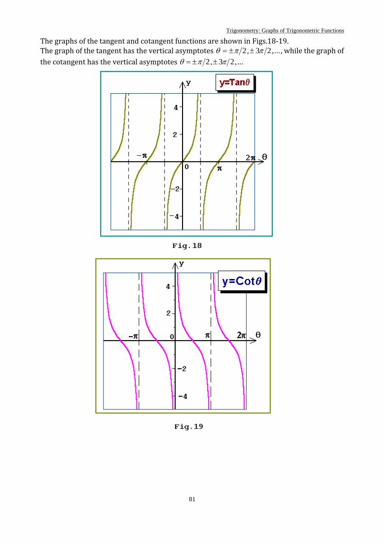
Trigonometry: Graphs of Trigonometric Functions
81
The graphs of the tangent and cotangent functions are shown in Figs.18‐19. The graph of the tangent has the vertical asymptotes ...,23,2 ππθ ±±= , while the graph of the cotangent has the vertical asymptotes ...,23,2 ππθ ±±=

Trigonometry: Graphs of Trigonometric Functions
82
11. Inverse Trigonometric Functions A function has an inverse function if there is one‐to‐one correspondence between its domain and range. Since trigonometric functions are periodic, so they do not have inverse functions. However, we can impose restrictions on the domain of the function so that an inverse function might exist.
Function
Symbol Domain Range Conditions
Inverse sine
xarcsinx1sin−
1|| ≤x 2
|arcsin| π≤x xx =)sin(arcsin
xx =− )sin(sin 1
Inverse cosine
xarccosx1cos−
1|| ≤x π≤≤ xarccos0 xx =)cos(arccos
xx =− )cos(cos 1 Inverse tangent
xarctanx1tan−
any Rx∈
2|arctan| π<x xx =)tan(arctan
xx =− )tan(tan 1
Inverse cotangent x1cot− any Rx∈ π<< − x1cot0 xx =− )cot(cot 1
The inverse cosecant and inverse secant are determined by the analogy with the above. The graphs of the inverse functions are shown in Figs. 20‐21.
Fig. 2021.

83
GEOMETRY
Geometry is the branch of mathematics that deals with the nature of space and the size, shape, and other properties of figures as well as the transformations that preserve these properties. Some assumptions in geometry are postulated without proof as a basis for reasoning or arguing. Postulates are propositions that require no proof, being self‐evident, or that are assumed true and used in the proof of other propositions. Theorems are theoretical propositions, statements or formulas that need to be proven first from other propositions or formulas before they can be used in a consequent proof. Every theorem consists of a hypothesis, i.e. the statement of the given facts, and a conclusion, i.e. the statement of what is to be proved. Postulates and theorems are used to prove geometric ideas. A proof can include a sequence of steps, statements, or demonstrations that leads to a valid conclusion. An indirect proof is such method when one assumes temporarily that the conclusion is false and reasons logically until a contradiction of the hypothesis or another fact is reached. QED is abbreviation for quod erat demonstrandum, used to denote the end of a proof.
1. Basic Terms of Geometry In geometry, the terms point, line and plane are considered to be undefined terms since they are explained using only examples and descriptions. These terms are useful in defining other geometric terms and properties. Points are the simplest figures in geometry. A point has no size, although it may represent an object with size. It is shown pictorially as a dot and is usually named using a capital letter. All geometric figures consist of points. A line is a set of points that originate from one point and extend indefinitely in two opposing directions. Often, a line is named by a lower case letter; if a line contains two points A and B, then the line can be denoted as AB or BA . Lines have no thickness, even though pictorial representations of lines do. Planes extend indefinitely in all directions and have no edges or thickness. Planes are often denoted by a single capital letter and represented as four‐sided figures. A halfplane is the part of a plane that lies on one side of a given line.
Space is the set of all points. Collinear points are points that lie in the same line. Coplanar points are points that lie in the same plane. The intersection of two geometric figures is the set of points that are common to both figures.

84
The intersection point of a line with a line or plane is called the foot of the line.
A locus is the set of all points that satisfy some specified requirement. A normal is the same as a perpendicular. The term “to bisect” means the same as to cut in half.
Postulates:
• Through two distinct points only one line can be drawn.
• Two straight lines can intersect in only one point.
• A point divides a line into two infinite subsets of points of the line. Each part of the line is called a halfline, and the dividing point is called the endpoint of each half‐line. If a half‐line contains its endpoint, it is said to be closed; if it does not, it is said to be open.
• A straight line divides the plane into three subsets of points: two half planes and the line itself.
• The intersection of two planes is a line.
• If two points are in a plane then the line through the points is in that plane.
• In a plane, one and only one line can be drawn through a point, either outside or on a given line, perpendicular to the given line.
• Through any three points, there is at least one plane, and through any three non‐collinear point there is exactly one plane.
• A line contains at least two points, a plane contains at least three points but not all in one line, and space contains at least four points, but not all on one plane.
• The shortest distance between two points is the length of the line segment joining them.
• A geometric figure can be moved without altering its size or shape.

85
Simple theorems:
The intersection of two lines is exactly at one point. If a line and a point not on the line are existent, then a plane contains both figures. If two lines intersect, then a plane contains both of them.
Segments
• A line segment is the part of a line between two given distinct points on that line (including the two points).
Segment AB consists of points A and B and all points in between A and B . A point C is said to be a point on the segment AB if
ABCBAC =+ . The points A and B are said to be endpoints of the segment AB .
• Congruent segments are segments with equal lengths.
• A chord is the line segment between two points on a given curve.
• The longest chord of a figure is called a diameter.
• The midpoint of a segment is the point that divides the segment into two congruent segments.
The point C is the midpoint of the segment AB because BCAC = .
• The ray AB is a set of points that originate from the point A and extend indefinitely in the direction to the point B .
The point A is the endpoint of the ray. When denoting a ray, its endpoint is named first.
• Two rays, AB and AC , are said to be opposite rays if they have a common endpoint and extend indefinitely in opposing directions.
All the points on both opposite rays are collinear with respect to each other.
• The bisector of a segment is a line, plane, ray or another segment that intersects the segment at its midpoint.
• A perpendicular bisector of a segment is a line, ray or another segment that is perpendicular to the segment at its midpoint. If a point lies on the perpendicular bisector of a segment, then the point is equidistant from the endpoints of the segment, and vice versa, if a point is equidistant from the endpoints of a segment, then the point lies on the perpendicular bisector of the segment.
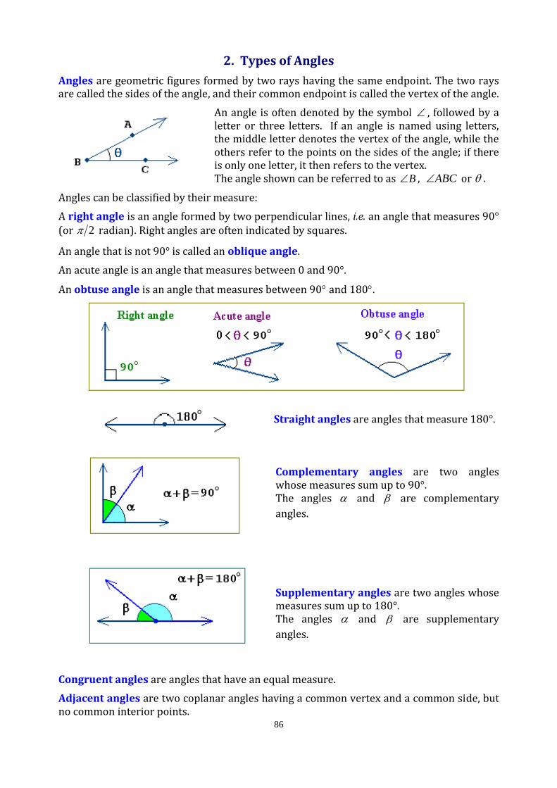
86
2. Types of Angles Angles are geometric figures formed by two rays having the same endpoint. The two rays are called the sides of the angle, and their common endpoint is called the vertex of the angle.
An angle is often denoted by the symbol ∠ , followed by a letter or three letters. If an angle is named using letters, the middle letter denotes the vertex of the angle, while the others refer to the points on the sides of the angle; if there is only one letter, it then refers to the vertex. The angle shown can be referred to as B∠ , ABC∠ or θ .
Angles can be classified by their measure: A right angle is an angle formed by two perpendicular lines, i.e. an angle that measures 90° (or 2π radian). Right angles are often indicated by squares.
An angle that is not 90° is called an oblique angle. An acute angle is an angle that measures between 0 and 90°.
An obtuse angle is an angle that measures between 90° and 180°.
Straight angles are angles that measure 180°.
Complementary angles are two angles whose measures sum up to 90°. The angles α and β are complementary angles.
Supplementary angles are two angles whose measures sum up to 180°. The angles α and β are supplementary angles.
Congruent angles are angles that have an equal measure. Adjacent angles are two coplanar angles having a common vertex and a common side, but no common interior points.
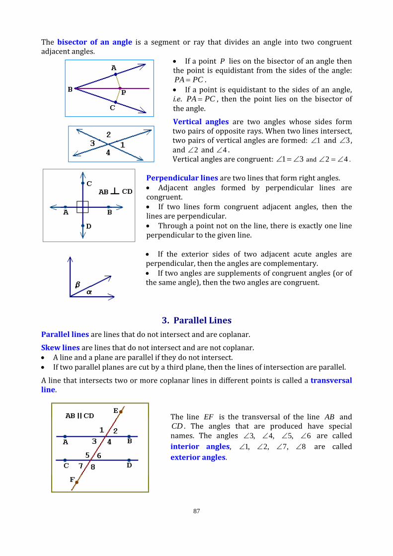
87
The bisector of an angle is a segment or ray that divides an angle into two congruent adjacent angles.
• If a point P lies on the bisector of an angle then the point is equidistant from the sides of the angle:
PCPA = . • If a point is equidistant to the sides of an angle, i.e. PCPA = , then the point lies on the bisector of the angle. Vertical angles are two angles whose sides form two pairs of opposite rays. When two lines intersect, two pairs of vertical angles are formed: 1∠ and 3∠ , and 2∠ and 4∠ . Vertical angles are congruent: 31 ∠=∠ and 42 ∠=∠ .
Perpendicular lines are two lines that form right angles. • Adjacent angles formed by perpendicular lines are congruent. • If two lines form congruent adjacent angles, then the lines are perpendicular. • Through a point not on the line, there is exactly one line perpendicular to the given line. • If the exterior sides of two adjacent acute angles are perpendicular, then the angles are complementary. • If two angles are supplements of congruent angles (or of the same angle), then the two angles are congruent.
3. Parallel Lines Parallel lines are lines that do not intersect and are coplanar. Skew lines are lines that do not intersect and are not coplanar. • A line and a plane are parallel if they do not intersect. • If two parallel planes are cut by a third plane, then the lines of intersection are parallel. A line that intersects two or more coplanar lines in different points is called a transversal line.
The line EF is the transversal of the line AB and CD . The angles that are produced have special names. The angles 6,5,4,3 ∠∠∠∠ are called interior angles, 8,7,2,1 ∠∠∠∠ are called exterior angles.

88
The two non‐adjacent interior angles on opposite sides of the transversal are called the alternate interior angles.
3∠ and 6∠ are alternate interior angles.
4∠ and 5∠ are alternate interior angles.
The two interior angles on the same side of the transversal are called the sameside interior angles.
3∠ and 5∠ are same‐side interior angles.
4∠ and 6∠ are same‐side interior angles.
The two angles in corresponding positions relative to the two lines are called the corresponding angles.
1∠ and 5∠ are corresponding angles.
2∠ and 6∠ are corresponding angles.
3∠ and 7∠ are corresponding angles.
4∠ and 8∠ are corresponding angles.
Postulates:
• If two parallel lines are intersected by a transversal, then the corresponding angles are congruent.
• If two lines are intersected by a transversal and their corresponding angles are congruent, then the lines are parallel.
Simple theorems:
If two parallel lines are intersected by a transversal, then the alternate interior angles are congruent.
If two parallel lines are intersected by a transversal, then the same‐side interior angles are supplementary.
If the transversal is perpendicular to one of the two parallel lines, then it is perpendicular to the other one as well.
If two lines are intersected by a transversal and their alternate interior angles are congruent, then the lines are parallel.
If two lines are intersected by a transversal and the same‐side interior angles are supplementary, then the lines are parallel.
In a plane, if two lines are perpendicular to the same line, then the lines are parallel. Through a point not on the line, there is exactly one line parallel to the given line. If two lines are parallel to a third line, then they are all parallel to each other. If three parallel lines cut congruent segments off a transversal, then they cut off congruent segments on every transversal.
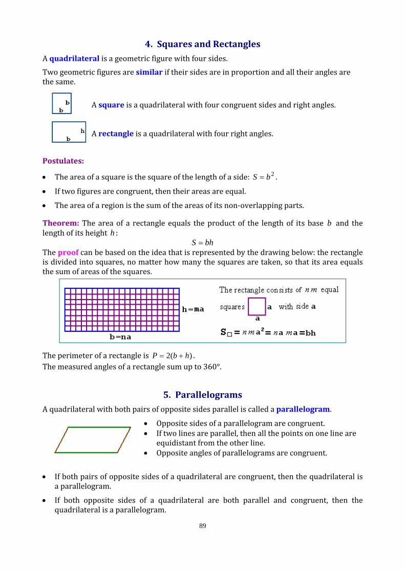
89
4. Squares and Rectangles A quadrilateral is a geometric figure with four sides. Two geometric figures are similar if their sides are in proportion and all their angles are the same.
A square is a quadrilateral with four congruent sides and right angles. A rectangle is a quadrilateral with four right angles.
Postulates:
• The area of a square is the square of the length of a side: 2bS = .
• If two figures are congruent, then their areas are equal.
• The area of a region is the sum of the areas of its non‐overlapping parts.
Theorem: The area of a rectangle equals the product of the length of its base b and the length of its height h :
bhS = The proof can be based on the idea that is represented by the drawing below: the rectangle is divided into squares, no matter how many the squares are taken, so that its area equals the sum of areas of the squares.
The perimeter of a rectangle is )(2 hbP += . The measured angles of a rectangle sum up to 360°.
5. Parallelograms A quadrilateral with both pairs of opposite sides parallel is called a parallelogram.
• Opposite sides of a parallelogram are congruent. • If two lines are parallel, then all the points on one line are
equidistant from the other line. • Opposite angles of parallelograms are congruent.
• If both pairs of opposite sides of a quadrilateral are congruent, then the quadrilateral is a parallelogram.
• If both opposite sides of a quadrilateral are both parallel and congruent, then the quadrilateral is a parallelogram.
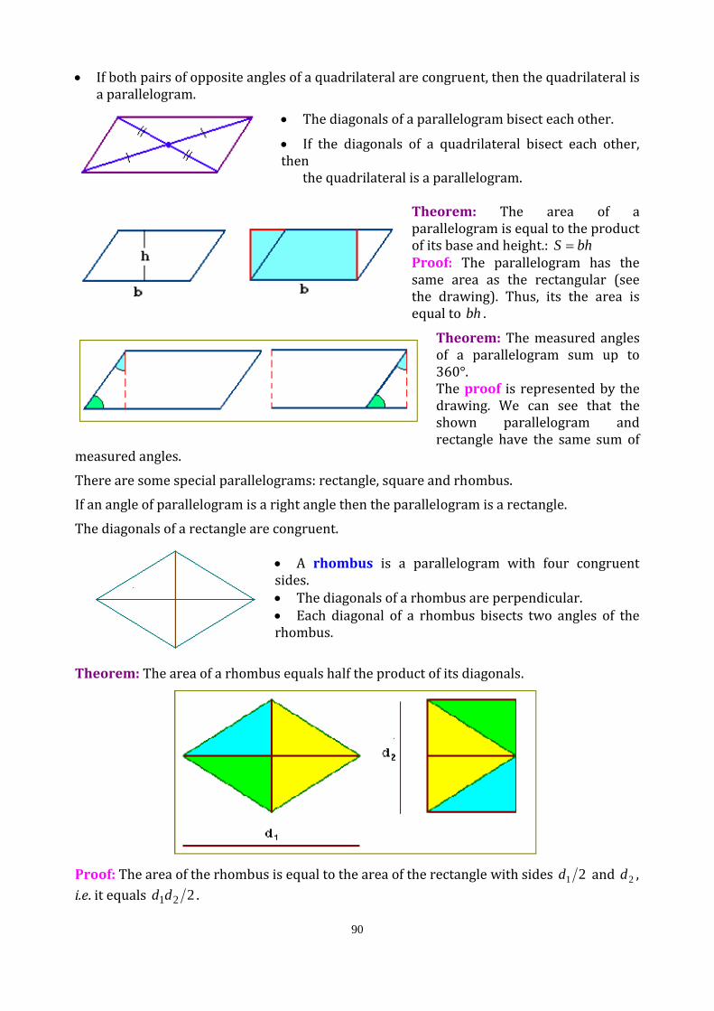
90
• If both pairs of opposite angles of a quadrilateral are congruent, then the quadrilateral is a parallelogram.
• The diagonals of a parallelogram bisect each other.
• If the diagonals of a quadrilateral bisect each other, then
the quadrilateral is a parallelogram.
Theorem: The area of a parallelogram is equal to the product of its base and height.: bhS = Proof: The parallelogram has the same area as the rectangular (see the drawing). Thus, its the area is equal to bh .
Theorem: The measured angles of a parallelogram sum up to 360°. The proof is represented by the drawing. We can see that the shown parallelogram and rectangle have the same sum of
measured angles. There are some special parallelograms: rectangle, square and rhombus. If an angle of parallelogram is a right angle then the parallelogram is a rectangle. The diagonals of a rectangle are congruent.
• A rhombus is a parallelogram with four congruent sides. • The diagonals of a rhombus are perpendicular. • Each diagonal of a rhombus bisects two angles of the rhombus.
Theorem: The area of a rhombus equals half the product of its diagonals.
Proof: The area of the rhombus is equal to the area of the rectangle with sides 21d and 2d , i.e. it equals 221dd .
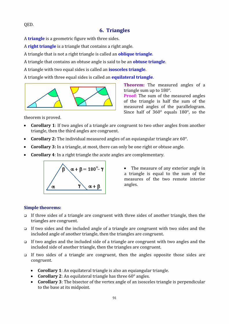
91
QED. 6. Triangles
A triangle is a geometric figure with three sides. A right triangle is a triangle that contains a right angle. A triangle that is not a right triangle is called an oblique triangle. A triangle that contains an obtuse angle is said to be an obtuse triangle. A triangle with two equal sides is called an isosceles triangle. A triangle with three equal sides is called an equilateral triangle.
Theorem: The measured angles of a triangle sum up to 180°. Proof: The sum of the measured angles of the triangle is half the sum of the measured angles of the parallelogram. Since half of 360° equals 180°, so the
theorem is proved.
• Corollary 1: If two angles of a triangle are congruent to two other angles from another triangle, then the third angles are congruent.
• Corollary 2: The individual measured angles of an equiangular triangle are 60°.
• Corollary 3: In a triangle, at most, there can only be one right or obtuse angle.
• Corollary 4: In a right triangle the acute angles are complementary. • The measure of any exterior angle in a triangle is equal to the sum of the measures of the two remote interior angles.
Simple theorems:
If three sides of a triangle are congruent with three sides of another triangle, then the triangles are congruent.
If two sides and the included angle of a triangle are congruent with two sides and the included angle of another triangle, then the triangles are congruent.
If two angles and the included side of a triangle are congruent with two angles and the included side of another triangle, then the triangles are congruent.
If two sides of a triangle are congruent, then the angles opposite those sides are congruent.
• Corollary 1: An equilateral triangle is also an equiangular triangle. • Corollary 2: An equilateral triangle has three 60° angles. • Corollary 3: The bisector of the vertex angle of an isosceles triangle is perpendicular
to the base at its midpoint.
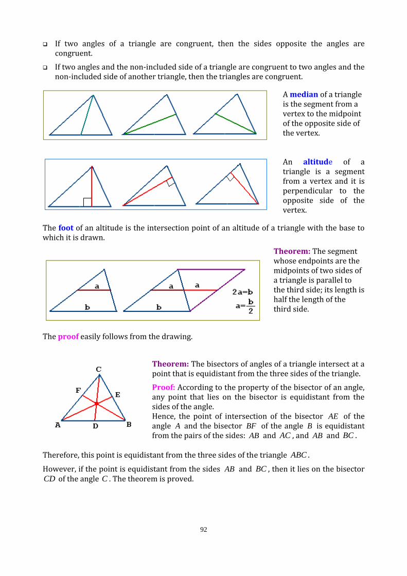
92
If two angles of a triangle are congruent, then the sides opposite the angles are congruent.
If two angles and the non‐included side of a triangle are congruent to two angles and the non‐included side of another triangle, then the triangles are congruent.
A median of a triangle is the segment from a vertex to the midpoint of the opposite side of the vertex.
An altitude of a triangle is a segment from a vertex and it is perpendicular to the opposite side of the vertex.
The foot of an altitude is the intersection point of an altitude of a triangle with the base to which it is drawn.
Theorem: The segment whose endpoints are the midpoints of two sides of a triangle is parallel to the third side; its length is half the length of the third side.
The proof easily follows from the drawing.
Theorem: The bisectors of angles of a triangle intersect at a point that is equidistant from the three sides of the triangle. Proof: According to the property of the bisector of an angle, any point that lies on the bisector is equidistant from the sides of the angle. Hence, the point of intersection of the bisector AE of the angle A and the bisector BF of the angle B is equidistant from the pairs of the sides: AB and AC , and AB and BC .
Therefore, this point is equidistant from the three sides of the triangle ABC .
However, if the point is equidistant from the sides AB and BC , then it lies on the bisector CD of the angle C . The theorem is proved.

93
Theorem: The perpendicular bisectors of the sides of a triangle intersect at a point that is equidistant from the three vertices of the triangle. Proof: According to the property of the bisector of a segment any point that lies on the perpendicular bisector of a segment is equidistant from the endpoints of the segment.
Hence, the point of intersection of the bisector OE of the segment BC and the bisector OFof the segment AC is equidistant from the pairs of the angles: A∠ and C∠ , and B∠ and
C∠ .
Therefore, this point is equidistant from the three vertices of the triangle ABC .
However, if the point O is equidistant from the endpoints of the segment AB , then this point lies on the perpendicular bisector OD of the segment AB . The theorem is proved.
Theorem: The lines that contain the altitudes of a triangle intersect at one point. Proof: Consider the triangle ABC . Let a point O be the point of intersection of the lines CO and EO that contain altitudes CD and EB respectively. Let us also draw the line AO . We have to prove that CFAO⊥ , i.e. the line AO contains altitude AF . 1) From the triangle AFC it follows that
)(180 CAFACFAFCAFB ∠+∠−°=∠=∠ . 2) Since ACFEBCOBF ∠−°=∠=∠ 90 , so we get from the triangle OBF
)(180 OBFFOBBFO ∠+∠−°=∠ ⇒ )(180)(180 ACBCAFACBBAFCABAFB ∠+∠−°=∠+∠+∠−°=∠
Theorem: The medians of a triangle intersect at a point that is two thirds the distance from a vertex to the midpoint of the side opposite the vertex. Proof: The median CD divides the triangle ABC into
two triangles, ADC and BDC . Let the segment EG be the median of the triangle BDC . If BF is the median of the triangle ABC , then parallel segments EG and CD divide this median into three equal parts so that FOBO 2= . Hence, the median CD intersects the median BF at the point O that is two thirds the distance from the vertex B to the midpoint F . In a similar way we can conclude that the median BF intersect the median CD at the point O that is two thirds the distance from a vertex C to the midpoint D .
The same conclusion is valid for any pairs of the medians. Therefore, the theorem is proved.

94
Theorem: The area of a triangle is equal to half the product of its base and height: 2/bhS =
Proof: The area of the triangle is equal to half the area of the parallelogram
with the same base and height.
Theorem: The area of a triangle with sides ba, and c can be calculated by using the following formula:
))()(( cpbpappS −−−= , where 2)( cbap ++= is half the perimeter of the triangle.
Similar Triangles
• If two angles of a triangle are congruent with two angles of another triangle, then the triangles are similar.
• If an angle of a triangle is congruent with another angle of a different triangle and their sides including the angles are in proportion, then the triangles are similar.
• If the sides of two triangles are in proportion, then the triangles are similar.
• If a line parallel to one of the sides of a triangle intersects the other two sides, then the line divides those sides proportionally.
• If a ray bisects an angle of a triangle, then it divides the opposite side of the angle into segments proportional to the other two sides.
7. Right Triangles In right triangles, the side opposite the right angle is called the hypotenuse, and the other sides are called the legs.
• If one side and the hypotenuse of a right triangle are congruent with the hypotenuse and one side of another right triangle, then the right triangles are congruent.
Theorem: The midpoint of the hypotenuse of a right triangle is equidistant from the three vertices. The proof follows from the drawing.
Theorem: The area of a triangle is the product of half the length of its base and the length of
the height: 2bhS =
Proof: It is clear from the above drawing that the area of a rectangle equals twice the area of a triangle on the one hand, and it equals the product bh of the length of the base and the length of the height on the other hand.

95
The Pythagorean Theorem: In a right triangle, the square of the hypotenuse is equal to the sum of the squares of the legs. 222 bac += .
Proof: It follows from the drawing that the area of the square with the sides )( ba + is equal to the sum of areas of the right triangles and the square with the sides c . The area of the right triangles with the
legs a and b is equal to 2ab .
However, according to the above postulate the area of the square is the square of the length of its side. Therefore,
22 )(2
4 bacab+=+⋅ ⇒
222 22 babacab ++=+ ⇒
222 bac +=
• If the square of one side of a triangle is equal to the sum of the squares of the other
sides, then the triangle is a right triangle.
• If the square of the longest side of a triangle is greater than the sum of the squares of the other two sides, then the triangle is an obtuse triangle.
• If the square of the longest side of a triangle is less than the sum of the squares of the other two sides, then the triangle is an acute triangle.
Special Right Triangles
An isosceles right triangle is also called a 45‐45‐90 triangle because of the measures of the angles. • The hypotenuse of a 45‐45‐90 triangle is 2 times as long as a leg.
• The hypotenuse of a 30‐60‐90 triangle is twice as long as the short leg and the longer leg is 3 times longer than the shorter leg.
8. Polygons Polygons are made by coplanar segments such that: • Each segment exactly intersects two other segments, one at each endpoint, • No two segments with a common endpoint are collinear. A Convex polygon is a polygon that has no side in the interior of the polygon. A polygon all of whose sides are equal is called an equilateral polygon. A polygon all of whose interior angles are equal is called an equiangular polygon. Polygons are named according to the number of sides they have. A triangle is the simplest polygon. The terms that apply to triangles can also be applied to polygons. The area of a polygon means the polygon itself and its interior.

96
A diagonal of a polygon is a segment that joins two non‐adjacent vertices. In the above drawing the dotted lines represent the diagonals of the polygon.
Polygons are similar if
• their corresponding vertices are congruent,
• their corresponding sides are in proportion.
Theorem: The sum of the measured angles of an n‐sided polygon is equal to the product °− 180)2(n .
Proof: Let us draw all diagonals of a polygon from one vertex to get the triangles (see the drawing). Since the number of the triangles is equal to )2( −n , and the sum of the measured angles of each triangle equals °180 , so the sum of the measured angles of an n‐sided polygon is equal to the product °− 180)2(n .
Examples:
• The number of sides of a triangle equals three. Therefore, °=°−=°− 180180)23(180)2(n .
• The sum of the measured angles of six‐sided polygon is equal to °=°− 720180)26( .
A regular polygon is a polygon that is both equilateral and equiangular. The regular six‐sided polygon is shown in the drawing.

97
9. Trapezoids
A quadrilateral with exactly one pair of parallel sides is a trapezoid. The parallel sides of a trapezoid are called bases, and the other sides are called legs. A trapezoid with congruent legs is called isosceles. Base angles of an isosceles trapezoid are congruent. Theorem: The median of a trapezoid • is parallel to the bases, • its length is equal to half the sum of the bases. Proof: The median of a trapezoid is equal to the sum of the medians of the parallelogram and triangle (see the drawing). The length of the median of the triangle equals half the sum of its base, i.e. 2)( ab − . Therefore, the length of the median of the trapezoid is 2)(2)( baaba +=−+ .
Theorem: The area of a trapezoid is equal to the product of half its height and the sum of the bases:
hbaS2+
=
Proof: The area of a trapezoid is equal to the sum of areas of the parallelogram and the triangle (see the above drawing). The area of the parallelogram is ah and the area of the triangle is equal to 2)( hab − . Therefore, the area of a trapezoid is
2)(2)( hbahabah +=−+ .
Corollary: Since the median of a trapezoid is equal to 2)( ba + , so the area of a trapezoid is equal to the product of its height and the median.
10. Geometric Inequalities
• If one side of a triangle is longer than a second side, then the angle opposite the longer side is larger than the opposite angle of the second side.
• If one angle of a triangle is larger than a second angle, then the side opposite the larger angle is longer than the opposite side of the second angle.
• Corollary 1: The perpendicular segment from a point to a line is the shortest segment from the point to the line.
• Corollary 2: The perpendicular segment from a point to a plane is the shortest segment from the point to the plane.
• The sum of the lengths of any two sides of a triangle is greater than the length of the third side.
• If two sides of a triangle are congruent with two sides of another triangle, but the included angle of the first triangle is larger than the included angle of the second

98
triangle, then the third side of the first triangle is longer than the third side of the second triangle.
• If two sides of a triangle are congruent with two sides of another triangle, but the third side of the first triangle is larger than the third side of the second triangle, then the included angle of the first triangle is larger than the included angle of the second triangle.
11. Circles
A circle is a set of points in a plane that are equidistant from a fixed point. The fixed point is called the center and the distance from the fixed point to the set of points is the radius. A segment that joins two points on a circle is called a chord. A chord that passes through the center is called a diameter. A secant is a straight line that intersects a curve in two or more points. The diameter of a circle is twice the radius.
Congruent circles are circles that have congruent radii. Concentric circles are circles in the same plane with the same center and different radii.
A circle is said to be circumscribed about the polygon, if the circle is drawn around a polygon and the vertices of the polygon are touching the circle A polygon is said to be inscribed in a circle, if the polygon is drawn inside the circle and the vertices of the polygon are touching the circle. meets a smooth curve at a single point and does not cut across the curve.
A tangent of a circle is the line that lies in the same plane as the circle and meets the circle at exactly one point, called the point of tangency, and does not cut across the curve.
• If a line is tangent to a circle then the radius is perpendicular to the line at the point of
tangency.
• If a line is perpendicular to the radius of a circle at the radius' outer endpoint, then the line is a tangent to the circle.
An arc is an unbroken part of a circle. A sector is a region that is bounded by two radii and an arc of the circle.
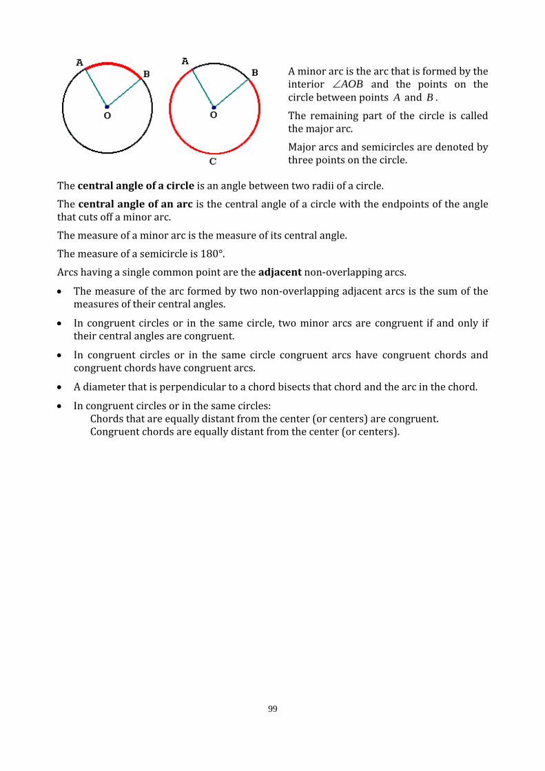
99
A minor arc is the arc that is formed by the interior AOB∠ and the points on the circle between points A and B . The remaining part of the circle is called the major arc. Major arcs and semicircles are denoted by three points on the circle.
The central angle of a circle is an angle between two radii of a circle. The central angle of an arc is the central angle of a circle with the endpoints of the angle that cuts off a minor arc. The measure of a minor arc is the measure of its central angle. The measure of a semicircle is 180°. Arcs having a single common point are the adjacent non‐overlapping arcs.
• The measure of the arc formed by two non‐overlapping adjacent arcs is the sum of the measures of their central angles.
• In congruent circles or in the same circle, two minor arcs are congruent if and only if their central angles are congruent.
• In congruent circles or in the same circle congruent arcs have congruent chords and congruent chords have congruent arcs.
• A diameter that is perpendicular to a chord bisects that chord and the arc in the chord.
• In congruent circles or in the same circles: Chords that are equally distant from the center (or centers) are congruent. Congruent chords are equally distant from the center (or centers).
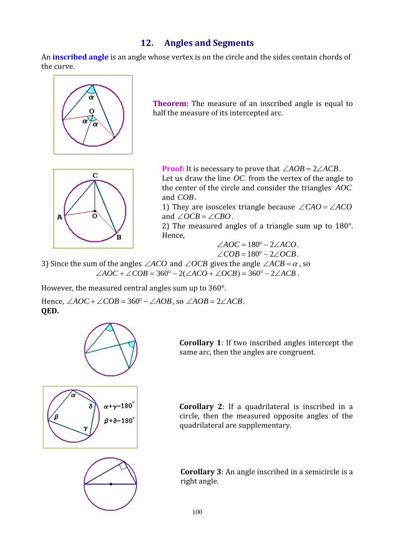
100
12. Angles and Segments
An inscribed angle is an angle whose vertex is on the circle and the sides contain chords of the curve.
Theorem: The measure of an inscribed angle is equal to half the measure of its intercepted arc. Proof: It is necessary to prove that ACBAOB ∠=∠ 2 . Let us draw the line OC from the vertex of the angle to the center of the circle and consider the triangles AOC and COB . 1) They are isosceles triangle because ACOCAO ∠=∠ and CBOOCB ∠=∠ . 2) The measured angles of a triangle sum up to 180°. Hence,
ACOAOC ∠−°=∠ 2180 . OCBCOB ∠−°=∠ 2180 .
3) Since the sum of the angles ACO∠ and OCB∠ gives the angle α=∠ACB , so ACBOCBACOCOBAOC ∠−°=∠+∠−°=∠+∠ 2360)(2360 .
However, the measured central angles sum up to 360°. Hence, AOBCOBAOC ∠−°=∠+∠ 360 , so ACBAOB ∠=∠ 2 . QED.
Corollary 1: If two inscribed angles intercept the same arc, then the angles are congruent.
Corollary 2: If a quadrilateral is inscribed in a circle, then the measured opposite angles of the quadrilateral are supplementary. Corollary 3: An angle inscribed in a semicircle is a right angle.
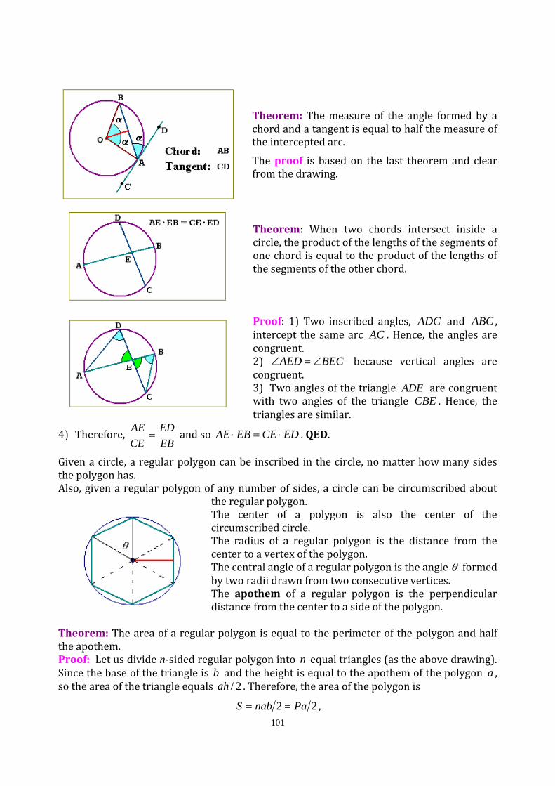
101
Theorem: The measure of the angle formed by a chord and a tangent is equal to half the measure of the intercepted arc. The proof is based on the last theorem and clear from the drawing.
Theorem: When two chords intersect inside a circle, the product of the lengths of the segments of one chord is equal to the product of the lengths of the segments of the other chord. Proof: 1) Two inscribed angles, ADC and ABC , intercept the same arc AC . Hence, the angles are congruent. 2) BECAED ∠=∠ because vertical angles are congruent. 3) Two angles of the triangle ADE are congruent with two angles of the triangle CBE . Hence, the triangles are similar.
4) Therefore, EBED
CEAE
= and so EDCEEBAE ⋅=⋅ . QED.
Given a circle, a regular polygon can be inscribed in the circle, no matter how many sides the polygon has. Also, given a regular polygon of any number of sides, a circle can be circumscribed about
the regular polygon. The center of a polygon is also the center of the circumscribed circle. The radius of a regular polygon is the distance from the center to a vertex of the polygon. The central angle of a regular polygon is the angle θ formed by two radii drawn from two consecutive vertices. The apothem of a regular polygon is the perpendicular distance from the center to a side of the polygon.
Theorem: The area of a regular polygon is equal to the perimeter of the polygon and half the apothem. Proof: Let us divide n‐sided regular polygon into n equal triangles (as the above drawing). Since the base of the triangle is b and the height is equal to the apothem of the polygon a , so the area of the triangle equals 2/ah . Therefore, the area of the polygon is
22 PanabS == ,
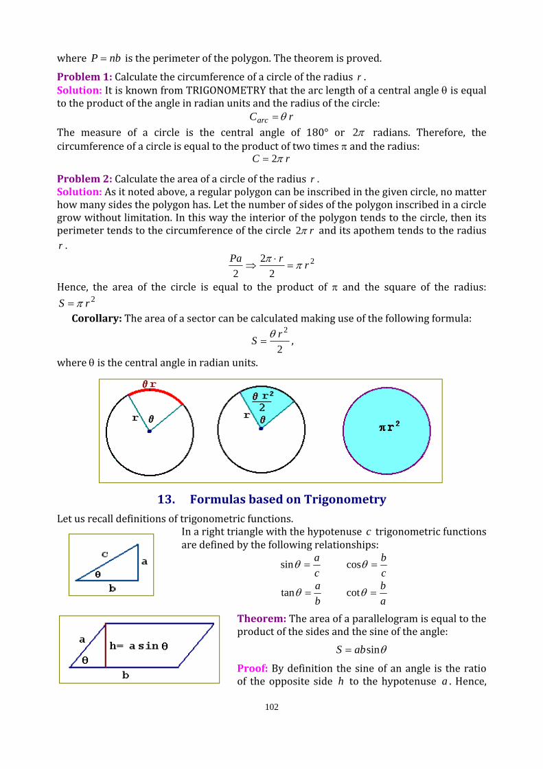
102
where nbP = is the perimeter of the polygon. The theorem is proved.
Problem 1: Calculate the circumference of a circle of the radius r . Solution: It is known from TRIGONOMETRY that the arc length of a central angle θ is equal to the product of the angle in radian units and the radius of the circle:
rCarc θ= The measure of a circle is the central angle of 180° or π2 radians. Therefore, the circumference of a circle is equal to the product of two times π and the radius:
rC π2=
Problem 2: Calculate the area of a circle of the radius r . Solution: As it noted above, a regular polygon can be inscribed in the given circle, no matter how many sides the polygon has. Let the number of sides of the polygon inscribed in a circle grow without limitation. In this way the interior of the polygon tends to the circle, then its perimeter tends to the circumference of the circle rπ2 and its apothem tends to the radius r .
2
22
2rrPa ππ
=⋅
⇒
Hence, the area of the circle is equal to the product of π and the square of the radius: 2rS π=
Corollary: The area of a sector can be calculated making use of the following formula:
2
2rS θ= ,
where θ is the central angle in radian units.
13. Formulas based on Trigonometry
Let us recall definitions of trigonometric functions. In a right triangle with the hypotenuse c trigonometric functions are defined by the following relationships:
ca
=θsin cb
=θcos
ba
=θtan ab
=θcot
Theorem: The area of a parallelogram is equal to the product of the sides and the sine of the angle:
θsinabS =
Proof: By definition the sine of an angle is the ratio of the opposite side h to the hypotenuse a . Hence,
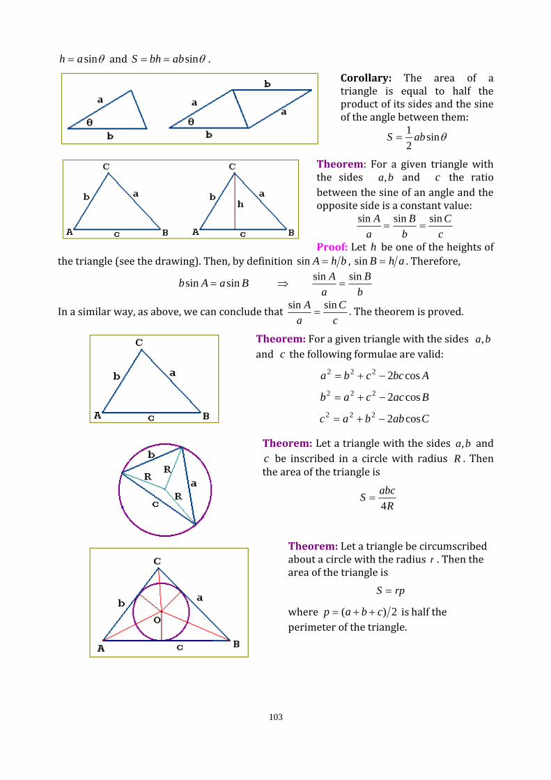
103
θsinah = and θsinabbhS == .
Corollary: The area of a triangle is equal to half the product of its sides and the sine of the angle between them:
θsin21 abS =
Theorem: For a given triangle with the sides ba, and c the ratio between the sine of an angle and the opposite side is a constant value:
cC
bB
aA sinsinsin
==
Proof: Let h be one of the heights of the triangle (see the drawing). Then, by definition bhA =sin , ahB =sin . Therefore,
BaAb sinsin = ⇒ b
Ba
A sinsin=
In a similar way, as above, we can conclude that cC
aA sinsin= . The theorem is proved.
Theorem: For a given triangle with the sides ba, and c the following formulae are valid:
Abccba cos2222 −+=
Baccab cos2222 −+=
Cabbac cos2222 −+=
Theorem: Let a triangle with the sides ba, and c be inscribed in a circle with radius R . Then the area of the triangle is
RabcS4
=
Theorem: Let a triangle be circumscribed about a circle with the radius r . Then the area of the triangle is
rpS =
where 2)( cbap ++= is half the perimeter of the triangle.
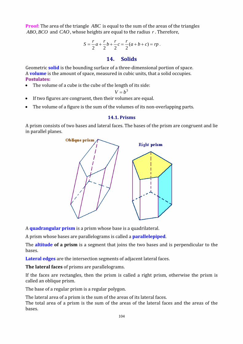
104
Proof: The area of the triangle ABC is equal to the sum of the areas of the triangles BCOABO, and CAO , whose heights are equal to the radius r . Therefore,
rpcbarcrbrarS =++=++= )(2222
.
14. Solids
Geometric solid is the bounding surface of a three‐dimensional portion of space. A volume is the amount of space, measured in cubic units, that a solid occupies. Postulates: • The volume of a cube is the cube of the length of its side:
3bV = • If two figures are congruent, then their volumes are equal.
• The volume of a figure is the sum of the volumes of its non‐overlapping parts.
14.1. Prisms
A prism consists of two bases and lateral faces. The bases of the prism are congruent and lie in parallel planes.
A quadrangular prism is a prism whose base is a quadrilateral. A prism whose bases are parallelograms is called a parallelepiped. The altitude of a prism is a segment that joins the two bases and is perpendicular to the bases. Lateral edges are the intersection segments of adjacent lateral faces. The lateral faces of prisms are parallelograms. If the faces are rectangles, then the prism is called a right prism, otherwise the prism is called an oblique prism. The base of a regular prism is a regular polygon. The lateral area of a prism is the sum of the areas of its lateral faces. The total area of a prism is the sum of the areas of the lateral faces and the areas of the bases.
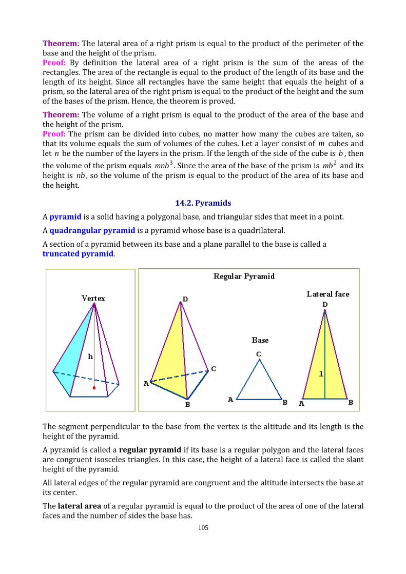
105
Theorem: The lateral area of a right prism is equal to the product of the perimeter of the base and the height of the prism. Proof: By definition the lateral area of a right prism is the sum of the areas of the rectangles. The area of the rectangle is equal to the product of the length of its base and the length of its height. Since all rectangles have the same height that equals the height of a prism, so the lateral area of the right prism is equal to the product of the height and the sum of the bases of the prism. Hence, the theorem is proved. Theorem: The volume of a right prism is equal to the product of the area of the base and the height of the prism. Proof: The prism can be divided into cubes, no matter how many the cubes are taken, so that its volume equals the sum of volumes of the cubes. Let a layer consist of m cubes and let n be the number of the layers in the prism. If the length of the side of the cube is b , then the volume of the prism equals 3mnb . Since the area of the base of the prism is 2mb and its height is nb , so the volume of the prism is equal to the product of the area of its base and the height.
14.2. Pyramids
A pyramid is a solid having a polygonal base, and triangular sides that meet in a point. A quadrangular pyramid is a pyramid whose base is a quadrilateral. A section of a pyramid between its base and a plane parallel to the base is called a truncated pyramid.
The segment perpendicular to the base from the vertex is the altitude and its length is the height of the pyramid. A pyramid is called a regular pyramid if its base is a regular polygon and the lateral faces are congruent isosceles triangles. In this case, the height of a lateral face is called the slant height of the pyramid. All lateral edges of the regular pyramid are congruent and the altitude intersects the base at its center. The lateral area of a regular pyramid is equal to the product of the area of one of the lateral faces and the number of sides the base has.
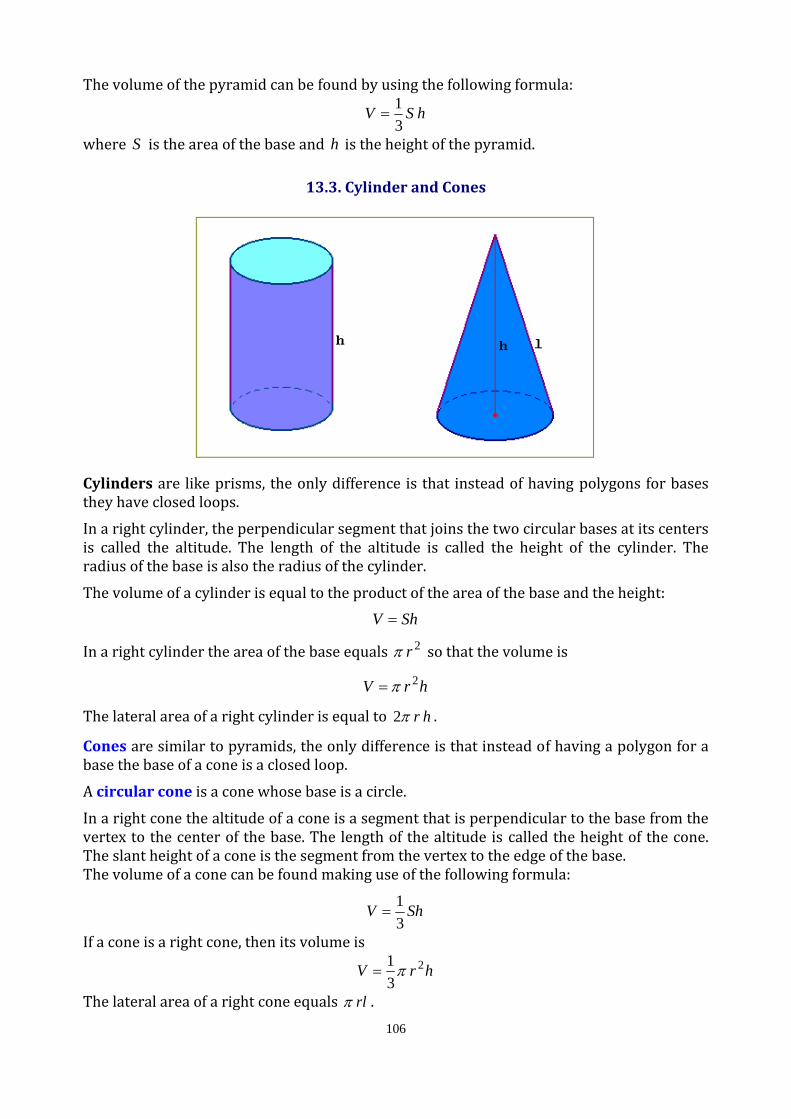
106
The volume of the pyramid can be found by using the following formula:
hSV31
=
where S is the area of the base and h is the height of the pyramid.
13.3. Cylinder and Cones
Cylinders are like prisms, the only difference is that instead of having polygons for bases they have closed loops. In a right cylinder, the perpendicular segment that joins the two circular bases at its centers is called the altitude. The length of the altitude is called the height of the cylinder. The radius of the base is also the radius of the cylinder. The volume of a cylinder is equal to the product of the area of the base and the height:
ShV =
In a right cylinder the area of the base equals 2rπ so that the volume is
hrV 2π=
The lateral area of a right cylinder is equal to hrπ2 .
Cones are similar to pyramids, the only difference is that instead of having a polygon for a base the base of a cone is a closed loop. A circular cone is a cone whose base is a circle. In a right cone the altitude of a cone is a segment that is perpendicular to the base from the vertex to the center of the base. The length of the altitude is called the height of the cone. The slant height of a cone is the segment from the vertex to the edge of the base. The volume of a cone can be found making use of the following formula:
ShV31
=
If a cone is a right cone, then its volume is
hrV 2
31π=
The lateral area of a right cone equals rlπ .

107
14.4. Spheres
A sphere is a locus of points in three‐ dimensional space that are equidistant from a fixed point (called the center). The terms used for circles are also used for spheres.
The area of a sphere with the radius r is equal to 24 rπ .
The volume of a sphere with the radius r is
3
34 rV π= .
Areas and volumes of similar solids If ba is the scale factor of two similar figures, then: • the ratio of the corresponding perimeters is ba ;
• the ratio of the lateral areas, base areas and total areas is 2)( ba ;
• the ratio of volumes is 3)( ba .
A solid of revolution is a solid formed by rotation a plane figure about an axis in three‐space.
References
1. D. Cohen. Precalculus. Minneapolis/St. Paul, N.Y., Los Angeles, San Francisco. 1997. 2. V.V. Konev, The Elements of Mathematics. Textbook. Tomsk. TPU Press, 2009, 140p. 3. V.V. Konev. The Elements of Mathematics. Workbook, Part 1. Tomsk. TPU Press, 2009,
54p. 4. V.V. Konev. The Elements of Mathematics. Workbook, Part 2. Tomsk. TPU Press, 2009,
40p. 5. V.V. Konev. Mathematics: Preparatory Course. Textbook. Tomsk. TPU Press, 1998, 104p.

Valery V. Konev, Associate Professor of the Higher Mathematics Department, TPU, Ph.D.
Preparatory course of Mathematics
Textbook Reviewed by: V.A. Kilin, Professor of the Higher Mathematics Department. TPU, D.Sc.


![Course Selection [Grade 11] - Crestwood Preparatory College](https://img.pdfslide.us/doc/110x75/6251e0fb3b45b96f755a9526/course-selection-grade-11-crestwood-preparatory-college.jpg)