PREPARATIVE DENSITY GRADIENT CENTRIFUGATIONS

By A. Fritsch Departement de Biologie Moleculaire

Institut Pasteur, Paris

Beckman®

for all countries except USA and Canada© Copyright by Beckman Instruments International S.A., Geneva,

CONTENTS

FOREWORD

5 CHAPTER I: INTRODUCTION

7 CHAPTER II: ZONE CENTRIFUGATION

9 II.1 The principle of the method 9 II.2 Practical aspects of zone centrifugation 10

a) The choice of the rotor b) The choice of the gradient material c) Making the gradient

- Swinging bucket rotors - Zonal rotors

d) Layering the macromolecular sample - Swinging bucket rotors - Zonal rotors

e) The centrifuge run f) Fractionating the gradient

II.3 The measurement of sedimentation coefficients 23 a) The sedimentation coefficient b) Isokinetic and equivolumetric gradients c) The measurement of sedimentation coefficients

II.4 Sedimentation coefficient and molecular weight 28 a) Proteins b) DNA's c) RNA's

II.5 Sedimentation and conformational changes 32 II.6 The resolving power 34

a) General notions b) Elements for a quantitative approach

- Isokinetic gradients - The gradient induced zone sharpening

II.7 The macromolecular load of the gradients 42 a) The hydrostatic stability criterion b) The differential diffusion effect c) The particular case of DNA

CHAPTER III: ISOPYCNIC CENTRIFUGATION 49 III.1 The principle of the method 49 III.2 The density gradient 50 III.3 Measurements and significance of the buoyant density 52 III.4 The shape of macromolecular bands 56 III.5 The duration of the centrifuge run 58

a) Sedimentation equilibrium of the gradient material b) Sedimentation equilibrium of the macromolecules

- Equilibrium gradients - Preformed gradients

III. 6 Resolving power, and rotor speed 62 a) Equilibrium gradients b) Preformed gradients

III.7 Density gradient materials and their applications 65 a) Nucleic acids b) Proteins c) Subcellular fractions d) Viruses e) Cells

III. 8 Practical aspects of isopycnic centrifugation 75

APPENDIX 79 A.1 Properties of rotors used for zone centrifugation A.2 Density of aqueous solutions of a few salts A.3 Sedimentation equilibrium coefficients of the aqueous solutions

of a few salts

A.4 Relationship between the density of salt solutions and their refractive index

BIBLIOGRAPHY 85

Foreword

Since the first edition of this monography, density gradient centrifugation methods have undergone numerous theoretical and technical improve-ments. In particular, the advent of high performance rotors, especially of zonal rotors, has led to a more thorough study of resolving power and macromolecular load of the gradients. Accordingly, the field of applications of these methods has been considerably extended. In addition to their being a fundamental tool in molecular biochemistry, they are more and more used for the fractionation and characterization of subcellular particles and whole cells. Their industrial applications have been developped as well.

Unavoidably, this second edition became almost a new book. But as for the first edition, its scope is limited to the use of density gradient methods with preparative centrifuges. They have not only their own methodology but their field of applications is the widest. Our aim was essentially to write a handbook which should help in setting up experiments and in interpreting their results.

If some properties, like the macromolecular load of the gradients, are in-completely treated, this is essentially because the experimental facts still suffer from a lack of good theoretical support. But as soon as this gap will be filled, one can predict that new experimental conditions will give rise to new applications. Other shortages of this text are exclusively due to the limits of our personal experience; we hope that we were able to compensate them partially by our choice of bibliographic references.

We are specially indebted to P. Tiollais for his criticism and invaluable sug-gestions during the preparation of the manuscript. We also acknowledge the help of P. Courvalin, P. Rouget, P. Tiollais and A. Ullmann who kindly supplied part of the experimental support. We wish especially to thank J. Freud for her expert secretarial contribution, and D. Thus/us for correcting the English translation.

Paris, February 1975.

CHAPTER I

Introduction

During density gradient* centrifugation, one should distinguish zone centrifugation (also called rate zonal centrifugation) from isopycnic centrifugation (or isopycnic zonal centrifugation). Despite the fact that one uses density gradients in both cases, that the macromolecules to be studied are always concentrated in narrow bands, and that one resorts to the same rotors, their principles are completely different. Zone centrifugation separates macromolecules according to their sedimentation velocity, or, more precisely, according to their sedimentation coefficients. The density of the sedimentation medium is always smaller than the density of the macromolecules. Accordingly, beyond a certain time of centrifugation, they will pile up at the bottom of the centrifuge tube, or at the edge of the rotor. The role of the gradient is secondary, albeit necessary: it is to avoid the convection currents which tend to destroy the macro-molecular zones. In the case of isopycnic centrifugation on the other hand, the density gradient constitutes the very principle of the method. The density range which is covered by the gradient, necessarily includes the density of the macromolecules. After a proper time of centrifugation the latter are concentrated at a position in the gradient where their density is equal to the density of the sedimentation medium. Isopycnic centrifugation, thus, separates macromolecules according to their density. Zone centrifugation and isopycnic centrifugation are semi-analytical meth- ods. Indeed, despite the impossibility to follow the sedimentation process while it is going on, one can measure sedimentation coefficients and den- sities, and sometimes molecular weights and conformational changes. The most remarkable aspect of both methods is that these parameters can be measured for non-purified macromolecules at extremely small amounts. The minimal amount depends on the sensitivity of the method used for measuring concentrations (enzymatic activity, radioactivity, etc.)] whereas the purity depends only on the specificity of this method for eadh kind of macromolecule. * In rigorous terms, the expression "density gradient" designates the slope of the curve which describes the density of the sedimentation medium as a function of the distance to the rotor axis. However, it is common practice in biochemistry to call density gradient every sedimentation medium in which a density change occurs. We shall use the expression in both senses, its precise meaning being always defined by the context.

Zone centrifugation and isopycnicc£nltifugation are also purification / methods at a more or less large scajefFor this application, the design (Ander-L--s"on and Burger, 1962) of the zonal rotors has led to large progress. In the laboratory, they allow the purification of several grams of ribosomal sub-units (Eikenberry et al., 1970), whereas a battery of 48 zonal centrifuges is used for the commercial purification of influenza vaccines (Sorrentino et al.,1973). The importance of zonal rotors is largely illustrated by an entire volume of Nat. Cancer Inst. Monograph (vol. 21, 1966), and by a recent meeting (Spectra 2000, vol. 4, 1973; Editions Cité Nouvelle, Paris) which entirely dealt with them.

Zone and isopycnic centrifugation methods can be combined, either as an analytical tool, for example to characterize the replicating complex of a viral genome (Magnusson et al., 1973), or as a preparative method for the purifi-cation of large amounts of subcellula£ fractions. For the latter, one takes into account that in the two dimensional space defined by the sedimentation coefficient and the density, mitochondria, nuclei, viruses, etc. occupy a very definite position (Anderson, 1966). Both methods are sometimes combined during the same centrifuge run (Wilcox et at., 1969: Anderson, 1973).

Our aim is to show how to use these centrifugation methods for both their analytical and preparative applications. Since it is impossible to mention all the applications, we will restrict ourselves to those which appear - at least to us - to be methodologically the most significant. Number of applications are analyzed in monographies devoted to zonal rotors (Anderson, 1967; Cline and Ryel, 1971; Price, 1972; Chervenka and Elrod, 1972) and in "Fractions" (Beckman Instruments, edt). In looking through any issue of the periodicals devoted to biochemistry, or molecular biology, one becomes rapidly aware of the variety, and of the importance of these methods.

CHAPTER II

Zone Centrifugation

11.1 THE PRINCIPLE OF THE METHOD

In order to separate macromolecules, or subcellular fractions according to their sedimentation coefficient differences, i.e. most often according to their mass differences (section II.3.a), two methods can be used. The first one, called moving boundary centrifugation, or differential centrifugation, consists in centrifuging a homogeneous solution of macromolecules. At the time where the most rapidly sedimenting molecules are pelleted at the bottom of the tubes, part of the more slowly sedimenting ones will still be in solution. If the ratio of the respective sedimentation velocities is equal to, say 5, the pellet will be contaminated by 20% of the slower macromolecules, whereas only less than 80% of them can be recovered in purified form.

The second method is zone centrifugation, still called rate zonal centrifuga-tion. After the pioneering work of Brakke (1951; 1953), Britten and Roberts (1960), and Martin and Ames (1961) gave zone centrifugation its present shape. Its principle is the following:

A very narrow layer, or zone, of a macromolecular solution is layered on top of an appropriate medium. During centrifugation, macromolecules with the same sedimentation velocity move through this medium as a single zone. It will appear as many zones as the initial layered contained different types of macromolecules. Each zone sediments at the speed characteristic of the macromolecules which it contains. The centrifuge run is stopped before the fastest zone has reached the bottom of the tube (or rotor). The content of the tube is then fractionated into layers perpendicular to the direction of the centrifugal force field, and the macromolecular content of each fraction is measured.

In order to keep the zones stable, i.e. as narrow as possible, their sedimentation should obey a certain number of criteria.

First, the density of the initial layer should always be smaller than the density of the sedimentation medium just below the layer. Otherwise, the content of the layer would immediately spread into the sedimentation medium.

Second, as soon as the macromolecular sample solution has been layered on top of the supporting medium, a negative density gradient is generated on the leading edge of the zone. In order to maintain the stability of the zone.

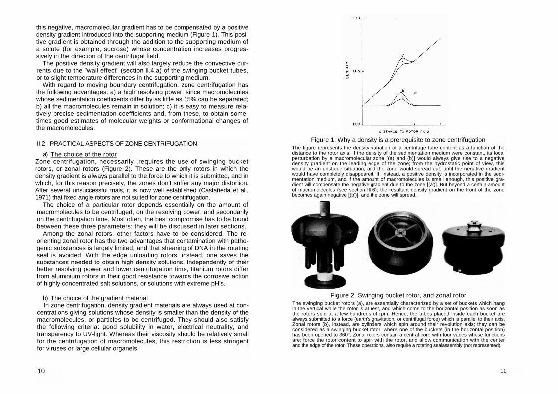
this negative, macromolecular gradient has to be compensated by a positive density gradient introduced into the supporting medium (Figure 1). This posi-tive gradient is obtained through the addition to the supporting medium of a solute (for example, sucrose) whose concentration increases progres-sively in the direction of the centrifugal field.

The positive density gradient will also largely reduce the convective cur-rents due to the "wall effect" (section ll.4.a) of the swinging bucket tubes, or to slight temperature differences in the supporting medium.

With regard to moving boundary centrifugation, zone centrifugation has the following advantages: a) a high resolving power, since macromolecules whose sedimentation coefficients differ by as little as 15% can be separated; b) all the macromolecules remain in solution; c) it is easy to measure rela-tively precise sedimentation coefficients and, from these, to obtain some-times good estimates of molecular weights or conformational changes of the macromolecules.

II.2 PRACTICAL ASPECTS OF ZONE CENTRIFUGATION a) The choice of the rotor

Zone centrifugation, necessarily .requires the use of swinging bucket rotors, or zonal rotors (Figure 2). These are the only rotors in which the density gradient is always parallel to the force to which it is submitted, and in which, for this reason precisely, the zones don't suffer any major distortion. After several unsuccessful trials, it is now well established (Castañeda et al., 1971) that fixed angle rotors are not suited for zone centrifugation.

The choice of a particular rotor depends essentially on the amount of macromolecules to be centrifuged, on the resolving power, and secondarily on the centrifugation time. Most often, the best compromise has to be found between these three parameters; they will be discussed in later sections.

Among the zonal rotors, other factors have to be considered. The re-orienting zonal rotor has the two advantages that contamination with patho-genic substances is largely limited, and that shearing of DNA in the rotating seal is avoided. With the edge unloading rotors, instead, one saves the substances needed to obtain high density solutions. Independently of their better resolving power and lower centrifugation time, titanium rotors differ from aluminium rotors in their good resistance towards the corrosive action of highly concentrated salt solutions, or solutions with extreme pH's.

b) The choice of the gradient material In zone centrifugation, density gradient materials are always used at con-

centrations giving solutions whose density is smaller than the density of the macromolecules, or particles to be centrifuged. They should also satisfy the following criteria: good solubility in water, electrical neutrality, and transparency to UV-light. Whereas their viscosity should be relatively small for the centrifugation of macromolecules, this restriction is less stringent for viruses or large cellular organels.

Figure 1. Why a density is a prerequisite to zone centrifugation The figure represents the density variation of a centrifuge tube content as a function of the distance to the rotor axis. If the density of the sedimentation medium were constant, its local perturbation by a macromolecular zone [(a) and (b)] would always give rise to a negative density gradient on the leading edge of the zone; from the hydrostatic point of view, this would be an unstable situation, and the zone would spread out, until the negative gradient would have completely disappeared. If, instead, a positive density is incorporated in the sedi-mentation medium, and if the amount of macromolecules is small enough, this positive gra-dient will compensate the negative gradient due to the zone [(a')]. But beyond a certain amount of macromolecules (see section III.6), the resultant density gradient on the front of the zone becomes again negative [(b')], and the zone will spread.

Figure 2. Swinging bucket rotor, and zonal rotor

The swinging bucket rotors (a), are essentially characterized by a set of buckets which hang in the vertical while the rotor is at rest, and which come to the horizontal position as soon as the rotors spin at a few hundreds of rpm. Hence, the tubes placed inside each bucket are always submitted to a force (earth's gravitation, or centrifugal force) which is parallel to their axis. Zonal rotors (b), instead, are cylinders which spin around their revolution axis; they can be considered as a swinging bucket rotor, where one of the buckets (in the horizontal position) has been opened to 360°. Zonal rotors contain a central core with four vanes whose functions are: force the rotor content to spin with the rotor, and allow communication with the center and the edge of the rotor. These operations, also require a rotating sealassembly (not represented).

10 11

Since the first experiments of Britten and Roberts (1960), the most used substance is sucrose. For certain experiments, it is necessary to usVglycerol, which is a distillation product, and thus devoid of impurities, in particular nucleases (Williams et al.,.1960; Orth and Cornwell, 1961). In order to\>btain a better resolving power than in sucrose, Kaempfer and Meselson N971) have used cesium chloride gradients at low temperature. For the centrifuga-tion of RNA, the use of sulfolane, trimethyl phosphate, or urea has been proposed (Parish and Hastings, 1S66; Hastings et al., 1968) the two former products have the advantage not toVteract with the liquid scintillation count-ing process. Centrifugation of DNA'xabove pH 12 leads to strand breaks, and in order to avoid them, Gaudin and Yielding (1972) centrifuge single stranded DNA in 90% to 100%, or 25% to\50% formamide gradients. Snyder et al. (1972) have studied the dissociation of alkaline phosphatase in Tris gradients. Sodium bromide gradients have been used for the fractionation of lipoproteins (Wilcox et al., 1969). Centrifugation of low molecular weight macromolecules (less than 104 daltons), leads to run lengths and rotor speeds which are such that the initial shape of the density gradient is modified (it tends towards the equilibrium gradient, see chapter III). Since zone centrifu-gation very often implies an accurate knowledge of the gradient shape (sections II.3 and II.4), McEwen (1967, a) suggests the use of equilibrium sodium chloride gradients; it is obvious that the macromolecules should then remain soluble, and stable at high ionic strength.

For the Centrifugation of subcellular particles sensitive to high osmotic pressure, sucrose can be replaced by sorbitol (Neal et al., 1970,1971), or by Ficoll (Boone et al., 1968; Pretlow, 1971). None of these two substances pene-trates into the cells. Ficoll solutions, at a weight to weight concentration of 25%, have an osmotic pressure similar to the physiological pressure. Mixtures of sucrose, sorbitol and Ficoll have also been used (Vasconcelos et al., 1971).

In all cases, the density gradient materialis dissolved in a buffer solution suited for each particular experiment. In order to increase the density of the solutions, they are sometimes prepared with heavy water (Beaufay et al., 1959; Kaempfer and MeselsorX 1971). \

In orderta solidify the conteYvt of the centrifuge tubes at the end of the centrifuge runTsome photopolymerizable acrylamide can be added to\the gradient (Cole, 1971). \

\ c) Making the gradient In this section, we shall only describe the methods used to obtain different

gradient shapes. Their properties, instead, will be given in later sections of this chapter.

- Swinging bucket rotors With this type of rotor, the gradients are established before centrifuga-

tion. They are obtained upon mixing in the proper way two solutions of the density gradient material at the appropriate concentrations. Before filling, the centrifuge tubes should sometimes be treated with silicone; this will

12

avoid sticking of the macromolecules on the tubes (Burgi and Hershey, 1968). It is recommended that the density gradient be established at the tempera-ture of the centrifuge run.

Figure 3 shows a very simple apparatus (Britten and Roberts, 1960; Martin and Ames, 1961), which is commercially available under different versions. It gives gradients in which the concentration of the gradient material varies linearly with distance, or certain convex gradients. More generally, if the two reservoirs, Ri and R2 have respective sections of Ai and A2 cm2, the shape of the gradient will be given by:

z1and z2 are the initial concentrations of the two gradient material solutions in each reservoir, and v1 and v2 are their initial volumes; z1and z2 are also the two extreme concentrations of the gradient, z is the concentration of the mixture when the centrifuge tube has received a gradient volume equal to v. (v1 + v2) is equal to the final gradient volume. Equation II-1 shows that the concentration varies linearly for A1 = A2. This case is the most widely used, especially in order to obtain the isokinetic (section II.3b) 5% to 20% sucrose, or 10% to 30% glycerol gradients, and for certain Ficoll gradients (Pretlow, 1971). For A1<A2, one obtains convex gradients with which the macro-molecular load can be increased (section II.7). The case where A1>A2 is

without any interest, since the density gradient at the meniscus would be equal to zero.

The apparatus of Figure 3 is more difficult to use when the density dif-

Figure 3. Density gradient maker for centrifuge tubes The gradients are constant, if the sections of both reservoirs are equal (see text).

II-1

ference between the two initial solutions is larger than 0.06 g/cm3, because the levels of the solutions in the two reservoirs would be different, and thus the gradient wouldn't have the expected shape. It is then easier to resort to the somewhat more complicated equipment (commercially available) in which two syringes are simultaneously emptied at the appropriate rate.

Figure 4 is a schematic representation of a very simple apparatus, with which exponential gradients are generated, i.e.

The various symbols of the equation are defined as above. With this ap-paratus, the volume V2 remains constant during the whole filling procedure of the centrifuge tube. Noll (1967,1969,1971), McCarty et al., (1968), Hender-son (1969) Leifer and Kreutzer (1971) give details for the construction of such apparatuses, as well as the method to determine the volume V2 and the initial concentrations in the two reservoirs. The same authors also show

Figure 4. Schematic representation of an exponential gradient maker

For its practical design, see the references given in the text.

14

how to obtain isokinetic gradients for sucrose concentrations at the meniscus larger than 5%. Henderson (1969) discusses the difficulties in setting up exponential gradients of large volumes.

Some other gradient apparatuses are sometimes used. The one described by Bessman (1967) is aimed to superimpose a series of gradients with de-creasing slopes. Niederwieser (1967) describes another one, with which concave, convex, or S-shaped gradients can be obtained.

Figures 3 and 4 have been drawn for the use of cellulose nitrate centrifuge tubes. With polyallomer tubes, which are not wetable, the solutions cannot flow along the tube wall. For this reason, these tubes have to be filled from the bottom: the gradient solution flows through a thin glass tube which touches the bottom of the centrifuge tube and filling starts with the less dense solution (in Figure 3, the mixture is made in the reservoir which con-tained initially the less dense solution). But polyallomer tubes can be rendered wetable if they stand for a few days in an "old" mixture of sulfochromic acid (Wallace, 1969).

For some particular applications (Cohen et al., 1972), continuous sucrose gradients have been obtained from a homogeneous solution which is sub-mitted to a few cycles of freezing and thawing.

As soon as the density gradients have been set up, the tubes and rotors have to be handled carefully. Mechanical shocks (extraction of the glass tube from polyallomer tubes), or sudden temperature variations, can severly perturb the gradient.

But, owing to the high viscosity of sucrose and glycerol solutions, the gradients can be stored in the cold for 12 or 24 hrs.

In order to avoid the collapse of the tubes during centrifugation, they have to be almost completely filled up: the filling volumes given in Table A.1 (appendix) leave an empty space of about 0.8 cm, which is enough for the plug used in the fractionation apparatus of Figure 7.

- Zonal rotors In reorienting zonal rotors, the gradient is established with the rotor at

rest. Apparatuses similar to those of Figures 3 and 4 can be used. With large extreme concentration differences of the gradient material, a "gradient pump" is more reliable (several models are commercially available): the gradient shape is generally given by a mechanical (Figure 5), or electronic cam. Any shape, even discontinuous gradients (Griffith and Wright, 1972), can be easily realized.

In certain cases, classical rotors can also be loaded at rest (Tayot and Montagnon, 1973).

More generally, the edge loading rotors have to be loaded while they are spinning at low speed (2,000 to 5,000 rpm), with filling rates of 20 to 40 ml/mn (Figure 6). In some cases, the procedures outlined in Figures 3 and 4 can be used, but due to the back-pressure generated in the rotating seal, a pump (peristaltatic pump) has to be inserted. Here again, a gradient pump is preferable. The connexions between the gradient pump and the

15

z - z1z2 - z1

= e-v/v2II-2

rotor should be as short as possible and their internal diameter about 2 mm (Price and Kovacs, 1969).

The instruction manuals of the rotors and pumps are very explicit and contain very detailed procedures. We shall only insist on the following point. Equations 11-1 and II-2 describe the concentration change of the gra-dient material as a function of the volume of the centrifuge tubes or rotors. In tubes, the concentration changes versus volume, or distance are identical. This is no longer true in zonal rotors, where the volume is a quadratic func-tion of the distance. Since the cam profile of the gradient pumps also de-scribes the concentration versus volume, this property has to be taken into account when the cams are prepared.

In the particular case of constant concentration gradients (the concentra-tion varies linearly with distance), the shape of the mechanical cam is given by: x and y are the relative coordinates of the cam profile; the abscissa x is pro-portional to the gradient volume, and, like y, varies from 0 to 1. a and b are dimensionless parameters, particular for each rotor, and are defined by:

Figure 5. Density gradient pump with a mechanical cam

a =

b =

Tb

®

Figure 6. Introduction of the density gradient in an edge loading zonal rotor

a) While the rotor is spinning at low speed, the gradient with increasing density is introduced at the edge (P), and the air is evacuated at the center (c).

b) Once the gradient fills the rotor, the sample solution is introduced through (c), and part of the bottom cushon of the gradient flows out of the rotor at the edge (P).

rm and rb are the distances from the rotor axis to the top and bottom of the gradient, respectively (typical values are given in Table A.1).

With such a cam, isokinetic gradients with a linear variation of 5% to 20% sucrose, or 10 to 30% glycerol are obtained. Steensgard (1970) has cal-culated the cam shapes which give isokinetic gradients for different mean sucrose concentrations, and different types of macromolecules.

With zonal rotors, other types of gradients appear to be more promising than isokinetic gradients.

We shall first mention the equivolumetric gradients, first set up by Price and his co-workers (Pollack and Price, 1971; Price, 1973). They have shown that with such gradients, sedimentation coefficients can be easily measured in zonal rotors (section Ill.S.b), and that a better resolving power is achieved (section II.6.b). For the practical make up of equivolumetric gradients the reader is referred to the following articles: Pollack and Price (1971); Berns et al. (1971); Van der Zeijst and Bult (1972); Eikenberry (1973); Schmider (1973). With equivolumetric gradients, Berns etal. (1971) obtained an excellent resolution upon the purification of calf crystalline lens messenger RNA, from the total polysomal RNA.

p c P C

x (b2-a2) + a21/2

-ay =II-3

rm

rb - rma =

rb

rb - rmb =

II-4

Figure 7. Fractionation device of density gradients in centrifuge tubes

The tube is firmly held in a clamp and connected to a water-manometer (M) through a three-way cock (R). While the rubber stopper is introduced into the centrifuge tube, the cock is open to atmospheric pressure. Then communication is made with the manometer, a negative pressure is applied above the tube whose bottom is then punctured with a needle (A). After removal of the needle the flowrate is kept at about one drop per second through a progressive increase of the pressure. Other devices are mentioned in the text.

®

Figure 8. Unloading of a zonal rotor At the end of the centrifuge run (a), the rotor speed is reduced to 2,000 to 5,000 rpm, and its content is fractionated (b) through the introduction of a sufficiently dense solution at the edge (P). The gradient flows out through the center (c) of the rotor.

18

Secondly, hyperbolic gradients should be mentioned. According to Ber-man (1966) they allow the centrifugation of maximal amounts of macro-molecules (section ll.6.a). Their shape is given by:

II-5

where ρ is the local density of the sedimentation medium, ρp the density of the macromolecules, r the distance to the rotor axis, and k a constant. Price (1972) gives details for the construction of these gradients. They have been used in the impressive work of Eikenberry etal. (1970), who separated in one single experiment, the subunits of 2 grams of ribosomes. They give the cam profile and the sucrose concentrations which they used for this work.

d) Layering the macromolecular solution onto the gradient Swinging bucket rotors

The small volume of macromolecular solution is layered on top of the gradient just before starting the run. Since the resolving power is greater the narrower the initial sample zone (section III.6), the great,est care should be taken in the layering procedure. To avoid any mixing with the gradient, a simple pipette or a mechanically driven syringe (Abelson and Thomas, 1966) with very low flow rates are suitable. Still another procedure is to use the specially designed band-forming caps (Cropper and Griffith, 1966). With DMA of very large molecular weight (more than 108 daltons) special precau-tions have to be taken (Levin and Hutchinson, 1973-a).

- Zonal rotors Once the gradient is established, the sample solution is simply layered

with a pipette (reorienting rotors), or with a large volume syringe connected to the central part of the rotor (rotor spinning at low speed). The syringe is emptied at a rate of 5 to 10 ml/mn (Figure 6,b).

In the case where large amounts of macromolecules have to be centrifuged (section III.7), it might be advantageous to introduce the sample as an in-verted gradient (Britten and Roberts, 1960; Eikenberry et al., 1970; Halsall and Schumaker, 1972). Instead of being constant throughout the initial sample layer, the macromolecular concentration increases from the "bottom" to the "top" of the layer. The inverted gradient is obtained with an apparatus similar to the one described in Figure 3; the flow into the rotor is facilitated with a pump, or with compressed air (Price and Hirvonen, 1967).

For both swinging bucket and zonal rotors, the problems of the initial width of the layer and of the macromolecular concentration will be dis-cussed below, in connection with the resolving power and the maximum macromolecular load.

e) The centrifuge run Except with DMA (see section II.4.b), all the rotors should be used at their

maximum allowable speed, since the resolving power is then the largest, and the centrifugation time the shortest.

19

ρ = ρp - kr

In order to determine the duration of the run the following has to be known: an estimate of the sedimentation coefficient of the most rapidly sedimenting zone; an estimate of the distance through which it has to move; certain properties of the gradient. With isokinetic (or equivolumetric) gradients, the duration can be determined with equation 11-11 (sections II.2.b and II.3.c) or from the K' constants given by the manufacturers of the rotors. With non-isokinetic gradients the centrifugation time can be estimated with curves similar to the one given in Figure 9. To achieve the best resolution, the centrifugation time will be set in order that the fastest zone will move as closely as possible to the bottom of the gradient.

In the cases where an accurate knowledge of the centrifugation time is required (measurement of sedimentation coefficients without an appropriate

Figure 9. Examples showing the isokinetic character of a 10% to 30%

glycerol gradient, and the non-isokinetic character of a 10% to 40% glycerol gradient, in the SW41 rotor

The relative distance (r- rm)/(rh- rm) through which a macro-molecular zone sediments at 5°C, has been plotted versus $20. w«?t. The different symbols are defined in the text.

Such curves allow the estimation of the centrifugation time: in order that macromolecules, characterized by SQQ.W = 20S, move through 85% of the length of the 10% to 40% gradient, one needs 520 ^ufl = 2.5; when the rotor is spun at its maximum speed (w2 = 1.84 x 107), it follows that t'= 2.5/20 x10~13x1.84 x107 = 6.8x104sec. #19 hours. For the same distance in the 10% to 30% gradient, one has S20.wurt = 2.05, and t = 19 (2.05/2.5) = 15.5 hours.

In the case of the non-isokinetic gradient, these curves also allow the estimation of sedi-mentation coefficients. If the 20S macromolecules are used as reference molecules, and if they have sedimented through 85% of the gradient length, one has u)2t = 2.5/20 x 10~13 = 1.25 x 10 . If the unknown macromolecules have sedimented through 68% of the gradient, it follows that S20.W"" = 1-88, and s'2o,w = 1.88/1.25 x 1012 = 15S. If this gradient were considered as an isokinetic one, one would obtain s'2o,w = 20 (68/85) = 16S, which would be in error by 7%. If this sedimentation coefficient were to be used for the determination of the molecular weight of DNA (equation 11-19), the figure found for the latter would be in excess of 20%.

20

• marker molecule; section II.3.c), the acceleration and deceleration times have to be taken into account. The equivalent sedimentation time during acceleration is given by:

Nmax is the working rotor speed in rpm, N its instantaneous speed and ∆t the time interval separating two consecutive speed values. As a rule, ten different speed values and the corresponding time intervals should be noted. A similar correction applies for the deceleration time tb. If t is the centrifuga-tion time at the working speed, the equivalent time of centrifugation is given by:

Another method to obtain teq is to use the special attachment on which the integral ‡ ω2dt can be read at any moment. This is actually the term which is necessary for the calculations; ω is the angular rotor speed in radians per second.

f) Fractionating the gradient Figure 7 shows a very simple set up, used to fractionate gradients in cel-

lulose nitrate or wetable (section II.2.c) polyallomer tubes. Similar devices are shown by Vinograd (1963). Their principle consists in puncturing the bottom of the tube with a needle, and then letting the tube content flow out dropwise; the flow-rate is controlled by a slight negative pressure above the tube. The drops are collected one by one, or by groups of several drops, into test tubes, scintillation vials, or on filters in view of their further analysis. The disadvantages of these devices are that the drop size is sometimes too large, or slightly variable.

They are eliminated if the tubes are punctured with a hollow needle, which is kept in place during the whole fractionation procedure. The drop size depends essentially on the outside diameter of the needle. A hollow needle has to be used whenever polyallomers have not been rendered wetable. Several such devices are commercially available. The most convenient ap-pear to be those where the point of the needle has lateral holes; this will avoid the needle from being plugged with an eventual precipitate or small tube debris due to puncturing.

To avoid the contamination of the collected fractions by a precipitate at the bottom of the gradient, the centrifuge tube can be punctured laterally with a syringe needle whose tip is pushed to the center of the tube.

Fractionation of the gradients from the top comes now more and more into use. It allows a better control of the different operations. A dense liquid is progressively injected at the bottom of the tube either via a hollow needle,

21

Sta =N2

max

1Nmax

0

N2∆t

teq = ta + t + tb

II-6

II-7

with which the tube bottom has been punctured, or via a thin rigid tube plunging through the gradient. The tube content is then pushed toward the top, where it flows through a specially designed stopper and the drops are collected by hand or by a fraction collector. While several such devices are commercially available, one of the most interesting ones has been designed by Bresch and Meyer (1973), since absolutely no mixing of consecutive gradient layers seems to occur, thus maintaining the maximum resolution. As a dense displacement liquid these authors recommend 1,1, 2, 2 - tetrabro-methane whose density is equal to 2.96 g/cm3.

If the concentration of the macromolecules and their extinction coefficient are large enough, their distribution through the gradient can be obtained with a continuous flow spectrophotometer.

The fractionation procedures of zonal rotors are explicitely outlined in the instruction manuals of the rotors (Figure 8). The flow rates at which the rotors are emptied should be kept relatively low, between 30 and 50 ml/mn. Fraction collection and the further analysis of their content can be done manually. But, owing to the large volume of zonal rotors, a recording con-tinuous flow spectrophotometer and a fraction collector are particularly usefull. To avoid any spreading of the zones during fractionation, the con-nections between the rotor outlet and the instruments to which it is connected should be kept as short as possible, and their internal diameter maintained at 2 mm (Price and Kivacs, 1969).

In the particular case where zone centrifugation is used to measure sedi-mentation coefficients, an accurate knowledge of the distance, or volume, through which this individual zones have moved, is required. This is relatively easy to determine in swinging bucket tubes: the distance is proportional to the number of constant volume fractions which separate a given zone from the less dense part of the tube content (section II.3.c).

This is no longer true in zonal rotors, where an overlay is layered on top of the initial sample zone. In order to determine the volume through which the zones have sedimented, one has to know which fraction corresponds to the interface initial sample/gradient. This interface can be determined through the measurement of the refraction index, i.e. gradient material con-centration, of each fraction. For this reason, a recording refractometer con-nected in series with the rotor outlet is particularly useful (use the second channel of the spectrophotometer recorder). 22

II.3 THE MEASUREMENT OF SEDIMENTATION COEFFICIENTS

a) The sedimentation coefficient The velocity at which a molecule sediments is characterized by its sedimenta-tion coefficient. It can be defined as the sedimentation velocity per unit field strength (Svedberg and Pedersen, 1940), i.e. r is the distance of the molecule to the rotor axis at time t; thus, dr/dt is its velocity at this time, ω is the angular rotor speed in radians/sec., and it is given by: where N is the rotor speed in rpm.

Sedimentation coefficients are usually expressed in Svedberg units; one Svedberg unit is equal to 10~13 CGS units, and its symbol is S.

The sedimentation coefficient of a given kind of macromolecule depends on properties of the macromolecule itself, as well on properties of the sedi-mentation medium. Svedberg and Pedersen (1940) have shown that: M is the molecular weight of the macromolecule, and f its frictional coef-ficient, which depends on the size and shape of the molecule and is always proportional to the local viscosity n of the sedimentation medium, ν is a parameter, which is obtained from the slope of a plot of sri versus p (Bruner and Vinograd, 1965), p being the local density of the sedimentation medium; in zone centrifugation, v differs only very slightly from the partial specific volume of the macromolecule, and it is as such that it will be designated in the following. (1-νρ) is called the buoyancy term. If it is positive, the macromolecules move in the direction of the centrifugal field, and in the opposite direction if it is negative. For (1 - νρ) = 0, no sedimentation occurs. NA is Avogadro's number.

Zone centrifugation separates macromolecules according to their sedi-mentation coefficients. According to equation II-9, it will be possible to separate macromolecules with different molecular weights, or macromolecules with the same mass but different conformations, or still, but very rarely, macromolecules with different partial specific volumes.

Equation II-9 shows also that the sedimentation coefficient s decreases for increasing density and/or viscosity of the sedimentation medium. In zone centrifugation both of these parameters increase continuously from the top

23

s =

drdtω2r

ω= 2π N60

II-9 s =M(1-νρ)

fNA

II-8

to the bottom of the gradient and they depend on the temperature. In addi-tion, sedimentation coefficients of different substances are rarely measured under identical experimental conditions (sedimentation medium, temperature). In order to take all these variations into account, Svedberg and Pedersen (1940) defined a standard sedimentation coefficient, 820, w, which one would measure in water at 20°C. 820, w is given by: where η20,w and (1-νρ)20,w are the viscosity of water, and the buoyancy term in water at 20°C. In addition to the gradient material, the contribution to r| and p of the salts of the sedimentation medium, is sometimes significant.

Experiments performed with an analytical centrifuge show that the stan-dard sedimentation coefficient decreases with increasing macromolecular concentration (Schachman, 1959); this variation is particularly important for DNA's (Crothers and Zimm, 1965). In order to obtain a sedimentation coef-ficient with a precise thermodynamic meaning (Tanford, 1961), the experi-mental values have to be extrapolated to zero concentration. The extrapolated sedimentation coefficient, designated by sº20,w. is a parameter characteristic of each type of macromolecule. Zone centrifugation is aimed to measure sº20,w values, too.

By this method, measurements are usually made at concentrations low enough to avoid any extrapolation. Nevertheless, with DNA zone centrifuga-tion leads to sedimentation coefficients slightly smaller than the values obtained from analytical centrifugation (Leighton and Rubenstein, 1969; Van der Schansetal., 1969; Levin and Hutchinson, 1973-a). If this difference can be explained by the difficulties to measure accurately absolute values of sedimentation coefficients by zone centrifugation, it is more likely due to the still non-understood interactions between DNA, density gradient mate-rial and water. In the following this difference will be neglected, and extrapo-lated sedimentation coefficients will be systematically designated by s20,w.

b) Isokinetic and equivolumetric gradients During sedimentation the macromolecules undergo two antagonistic ef-

fects: their sedimentation velocity tends to increase, due to the progressive increase of the centrifugal field; simultaneously, they move through a medium of increasing density and viscosity, which tends to decrease their velocity. Thus, the sedimentation velocity of the macromolecules is not necessarily constant (equation 11-10); the way it varies with distance depends on the rotor, on the composition and shape of the gradient and on the temperature.

In addition, zone centrifugation allows only the measurement of an average sedimentation velocity, which is calculated from the total distance through which the macromolecules have sedimented, and from the length of the run.

24

Finally, the measurement of standard sedimentation coefficients by zone centrifugation requires the search for conditions which give the simplest relation between sedimentation coefficient and sedimented distance. The fact that the gradient is fractionated into constant volume fractions will have to be taken into account. The simplest relation will then be the one where the number of fractions through which the molecules have moved during a given time, is proportional to their standard sedimentation coefficient.

In the cylindrical tubes of the swinging bucket rotors, the number of con-stant volume fractions through which a zone has moved, is proportional to the sedimented distance. For this type of rotor, the ideal conditions will be those where this distance is proportional to s20,w. According to equation 11-10, it will also be proportional to the duration of the centrifugation time, and to the square of the angular rotor speed tu. That is, where α is a proportionality constant, rm the distance of the meniscus to the rotor axis, and r the distance to the same axis of the macromolecular zone at time t. The sedimentation velocity will then be constant and equal to αs20,wω2. A medium in which the sedimentation velocity is constant, is called an isokinetic gradient. Equation 11-11 can be written under a more practical form, which is: where rb is the distance of the bottom of the gradient to the rotor axis, S20,w the standard sedimentation coefficient in Svedberg units, N0 the rotor speed in thousands of rpm, t' the centrifugation time in hours, and a^ a new constant (table A.1 of the appendix); the first member of the equation is equal to the fractional length of the gradient through which the macromolecular zone has moved.

Martin and Ames (1961), in the case of proteins, and Burgi and Hershey (1963), in the case of double-stranded linear DNA, were the first to show that, with the SW39 rotor, sucrose gradients whose concentration varies linearly from 5% to 20%, are indeed isokinetic gradients. This result has later been largely confirmed by others (Siegel and Monty, 1966; Abelson and_ Thomas, 1966; Van der Schans et al., 1969). It has then been extended to all the swinging bucket and zonal rotors, to glycerol gradients whose con-centration varies linearly between 10% and 30%, and the corresponding a-values have been calculated (Fritsch, 1973-b).

Isokinetic sucrose gradients can also be obtained for any value of the sucrose concentration at the meniscus, provided the sucrose concentration in the gradient varies exponentially (section II.2.c). Isokinetic Ficoll gradients have also been set up (Pretlow, 1971).

With constant concentration gradients, the isokinetic character is lost if the extreme concentrations are different from 5% and 20% sucrose, or 10% and 30% glycerol (Siegel and Monty, 1966; Fritsch, 1973-b). Examples are

s20,w =

drdtω2r

x ηη20,w

xνρ(1 - )20,w

νρ(1 - )II-10

r - rm = αs20,w ω2tII-11

r - rmrb - rm

= αS20,wN2t’ºII-11bis

given in Figures 9 and 13. Since in zonal rotors, the volume increases with the square of the radius,

with isokinetic gradients the sedimented distance will not be proportional to the number of constant volume fractions through which the zones move. For this type of rotors, the ideal conditions for measuring standard sedimen-tation coefficients will then be those where the volume - and no more the distance - through which the macromolecules have moved, is proportional to Sao.w. Gradients with this property are called equivolumetric gradients (Pollack and Price, 1971; Price, 1973-a).

c) The measurement of the sedimentation coefficient According to the type of rotor to be chosen for the experiment, isokinetic

or equivolumetric gradients will be preferentially used. If the aim of the experiment is only to measure sedimentation coefficients, a small swinging bucket rotor will be the most appropriate. These rotors have the best resolving power, and the shortest centrifugation time. Except in certain cases (section ll.4.b), they should be used at their maximum speed. The macromolecular concentrations should be small enough to avoid any extrapolation to zero concentration. This implies the availability of a sufficiently sensitive method to measure the concentrations in the individual fractions (enzymatic activity, radioactivity, etc.).

The centrifugation time will be chosen in order that the most rapidly sedimenting zone will move close to the bottom of the gradient. If an estimate of the corresponding sedimentation coefficient is available, the length of the run can be determined from equation 11-11 bis. The necessary values of a can be found in Table A.1. The centrifugation time can also be determined with the K'values given by the manufacturers of the rotors.

Since the sedimentation coefficient of an unknown substance is propor-tional to the number of constant volume fractions through which the cor-responding zone has sedimented, the simplest way to measure it, is to centrifuge a mixture of this substance and of a similar one (two proteins, two DNA's, etc.) whose sedimentation coefficient is known. If the known sedimentation coefficient is equal to (520, w)i, the coefficient to be measured will be given by where n1 and n2 are the number of fractions through which the known and unknown macromolecules have respectively sedimented.

In the experiment of Figure 10, one has n1 = 37 - 24 = 13, and n2 = 37 -19 = 18; knowing that (s20,w)1 = 11.4S, one gets (S20,w)2 = 11.4 (18/13) = 15.8S.

Since it is standard sedimentation coefficients which one wants to mea-sure, the reference macromolecules and the unknown macromolecules need to have the same partial specific volume ν. Martin and Ames (1961) have shown that with the assumption that a certain RNA has the same partial

26

specific volume as the reference proteins (0.72 cm3/g), one gets s20,w = 4.6S, whereas if the correct value of ν is taken (0.48 cm3/g), one gets s20,w = 4.4 S.

More generally, it has been shown (Fritsch, 1973-b), that the a and a con-stants of equation 11-11 relative to nucleic acids, are 7% larger than those relative to proteins.

As a rule, the sedimentation coefficients of the reference and unknown macromolecules should not differ by more than a factor of two. Standard sedimentation coefficients of numerous proteins and nucleic acids are pub-lished in the "Handbook of Biochemistry" (Sober, edit, the Chemical Rubber Co.).

According to equations II-11, sedimentation coefficients can be measured without a marker substance. But then, the proportionality constant, a or a, the duration of the centrifugation, the rotor speed, and the sedimented distance have to be known with a relatively good accuracy. This is relatively easy for the last parameter, but, in current practice, more delicate for the others. More particularly, the actual value of a is extremely sensitive to tem-perature (3% to 4% variation per degree centigrade; see table A.1), which is not always well known. In addition, the actual rotor speed is not always equal to the value given on the centrifuge; finally, the speed variations during the acceleration and braking periods of the rotor should also be taken into account (section II.2.c).

At least in principle, sedimentation coefficients can also be measured in non-isokinetic (or, non-equivolumetric) gradients. In addition to the preceding difficulties, one should add the exact knowledge of how the sedimented

Figure 10. Zone centrifugation of a mixture of catalase (•) and {3-galactosidase (o)

The experiment has been performed in an SW39 rotor, at 5°C. 39,000 rpm, and the run time was 7 hours. The centrifuge tube contained 4.8 ml of a constant 5% to 20% sucrose gradient, over which a 0.1 ml sample solution was layered. At the end of the run, the tube was punctured at the bottom and the gradient was fractionated into 37, identical 5 drops fractions. The enzymatic activity (arbitrary units) was plotted versus the fraction number. (The experimental results were kindly supplied by A. Ullmann.)

27

(s20,w)2 = (s20,w)1 xn2n1

II-12

distance (or volume) varies with time. This can be obtained from an experi-mental calibration of the gradients (Reisner et al., 1972), or through compu-tation (Bishop, 1966; McEwen, 1967b), or still from curves similar to those of Figure 9.

The sedimentation coefficients of subcellular particles can be measured by moving boundary centrifugation in swinging bucket rotors (Slinde and Flatmark, 1973).

II.4 SEDIMENTATION COEFFICIENT AND MOLECULAR WEIGHT

If the sedimentation coefficient of a given macromolecule depends on its molecular weight, it also depends on the frictional coefficient and on the partial specific volume (equation II-9), i.e. on the overall conformation of the macromolecule. In general, it will be impossible to determine molecular weights from the only measurement of sedimentation coefficients.

But one of the most interesting properties of zone centrifugation is that sedimentation coefficients can be measured with non purified substances, at very low concentration. For this reason the problem of the molecular weight determination of such substances, has arisen since the very first applications of the method (Martin and Ames, 1961; Burgi and Hershey, 1963).

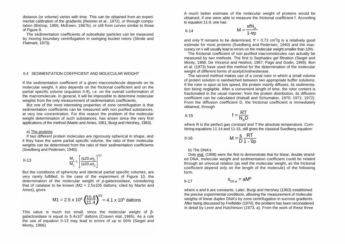
a) The proteins If two different protein molecules are rigorously spherical in shape, and

if they have the same partial specific volume, the ratio of their molecular weights can be determined from the ratio of their sedimentation coefficients (Svedberg and Pedersen, 1940): But the conditions of sphericity and identical partial specific volumes, are very rarely fulfilled. In the case of the experiment of Figure 10, the determination of the molecular weight of p-galactosidase, considering that of catalase to be known (M2 = 2.5x105 daltons; cited by Martin and Ames), gives This value is much too small, since the molecular weight of β-galactosidase is equal to 5.4x105 daltons (Craven etal.,1965). As a rule the use of equation II-13 may lead to errors of up to 50% (Siegel and Monty, 1966).

A much better estimate of the molecular weight of proteins would be obtained, if one were able to measure the frictional coefficient f. According to equation 11-9, one has:

and only ν remains to be determined, ν = 0,73 cm3/g is a relatively good estimate for most proteins (Svedberg and Pedersen, 1940) and the inac-curacy on v will usually lead to errors on the molecular weight smaller than 10%.

The frictional coefficient of non purified macromolecules can actually be measured by two methods. The first is Sephadex gel filtration (Siegel and Monty, 1966; De Vincenzi and Hedrick, 1967; Page and Godin, 1969). Bon et al. (1973) have used this method for the determination of the molecular weight of different forms of acetylcholinesterase.

The second method makes use of a zonal rotor in which a small volume of protein solution is sandwiched between two appropriate buffer solutions. If the rotor is spun at low speed, the protein mainly diffuses, its sedimenta-tion being negligible. After a convenient length of time, the rotor content is fractionated in the usual manner; from the protein distribution, its diffusion coefficient can be calculated (Halsall and Schumaker, 1970; 1971; 1972). From the diffusion coefficient D, the frictional coefficient is immediately obtained, through where R is the perfect gas constant and T the absolute temperature. Com-bining equations 11-14 and 11-15, still gives the classical Svedberg equation:

b) The DNA's Doty etal. (1958) were the first to demonstrate that for linear, double strand-

ed DNA, molecular weight and sedimentation coefficient could be related through an univocal relation (as well the molecular weight, as the frictional coefficient depend only on the length of the molecule) of the following form: where a and b are constants. Later, Burgi and Hershey (1963) established the precise experimental conditions, allowing the measurement of molecular weights of linear duplex DNA's by zone centrifugation in sucrose gradients. After being discussed by Freifelder (1970), the problem has been reconsidered in detail by Levin and Hutchinson (1973, a). From the work of these three

M1M2

=(s20,w)1(s20,w)2

3/2

II-13

M =sfNA

1-νρII-14

f = RTNADII-15

M1 = 2.5 x 105 15.811.4( )3/2

= 4.1 x 105 daltons

M = sD

RT1 - νρ

II-16

s20,w = aMbII-17

groups, it appears that if the centrifugation is performed in 5% to 20% sucrose gradients, containing IM NaCI, 10-2 M Tris, and 3.5.10-3 M EDTA, in a small swinging bucket rotor, at speeds below 35,000 rpm, and for 4.3x106< M < 110x106daltons, one has: with s20,w given in Svedberg units.

With isokinetic gradients, and if n1 and n2 are the number of fractions through which two DNA's with molecular weights M1 and M2 have moved, equation 11-18 reduces to: This allows an easy measurement of one of the molecular weights, if the other one is known.

Equations similar to II-18 and II-19 hold for linear, single-stranded DNA. Abelson and Thomas (1966), and Levin and Hutchinson (1973, b) have shown that in constant 5% to 20% sucrose gradients, containing 0.9M NaCI and 0.1 NaOH,one has

For circular DNA's, Clayton and Vinograd (1967) have established equa-tions similar to 11-17. They found: b = 0.38 for double-stranded, circular, supercoiled DNA (pH 7) b = 0.39 for double-stranded, circular, relaxed DNA (pH 7) b = 0.49 for double-stranded, alkaline denatured, supercoiled DNA (the pH of the sedimentation medium has to be equal to 12, or above).

These last three values of b have been determined by analytical centrifuga-tion and they still seem to be checked by zone centrifugation.

Centrifugation of linear duplex DNA raises a problem particular to this type of molecule. It has been recognized for a long time (see, for example Aten and Cohen, 1965), that beyond a certain rotor speed, the sedimenta-tion coefficient of a given DNA decreases, instead of remaining constant. The limiting rotor speed is the smaller, the larger the molecular weight of the DNA.

Levin and Hutchinson (1973, a) have studied this phenomenon while they isolated the intact B. subtilis chromosome through zone centrifugation. They rely upon a theoretical study of Zimm, who shows that if a DNA molecule sediments through a viscous liquid and if the rotor speed is progressively increased, the molecule undergoes a conformational change, passing from a random coil structure to a structure with a smaller sedimentation coefficient.

These authors show that in order to keep equations 11-18 and 11-19 ap-

plicable, a DNA of 110x106 daltons (DNA from bacteriophage T2) has to be centrifuged at less than 37,000 rpm, if constant 5% to 20% sucrose gra-dients and the SW50.1 rotor are used. One calculates that for the same experimental conditions, a DNA of 78x106 daltons has to be spun at less than 55,000 rpm, and a DNA of 30x106 daltons at less than 100,000 rpm (this speed is far beyond the upper limit of the presently available rotors). During the course of their study, Levin and Hutchinson (1973, a) showed that for increasing molecular weight of the DNA's, the sedimentation velocity reaches an upper limit. Particularly, if they apply equation 11-19 to the entire chromosome of B. subtilis using T2 DNA as a reference, and centrifuging at 7,400 rpm, they can only conclude that the chromosomal DNA is equal or greater than 13 times the T2 DNA. They show by another method that, in fact, the B. subtilis chromosome is 26.4 times longer than the T2 DNA.

Circular DNA's, or single stranded DNA have a more compact structure than linear duplex DNA's of the same length - for this reason they sediment faster - and it seems likely that their conformation will be less affected by sedimentation. But it seems safe to use the same rotor speed limitations.

c) The RNA's The measurement of the molecular weight of RNA's raises the same

problem as for proteins. The conformations of tRNA, mRNA, etc. are very different from each other, and no univocal relation between sedimentation coefficient and molecular weight exists (Boedtker, 1968).

Nevertheless, in the case of single-stranded RNA and in the absence of intra- and intermolecular interactions, an equation similar to equation 11-17 could be established (Gierer, 1958; Spirin, 1961). In constant 5% to 20% sucrose gradients, containing 10~1M NaCI, and 10~2M EDTA, the two authors find respectively: a = 1,100 b = 2.2 a = 1,550 b = 2.1

According to Staehelin etal. (1964), the coefficients of Gierer are the most accurate.

More generally, the molecular weight measurement of non-purified RNA's requires the measurement of their frictional coefficients. It seems that the method of Halsall and Schumaker (1972; see also section IIAa) should be the most reliable.

30 31

s20,w = 0.506 M0.38

n1n2

= ( )M1M2

0.38

II-18

II-19

n1n2

= ( )M1M2

0.39

II-20

11.5 SEDIMENTATION COEFFICIENT AND CONFORMATIONAL CHANGE

According to equation 11-9, the sedimentation coefficient depends on the frictional coefficient and on the partial specific volume, i.e. on the conforma-tion of the macromolecule. Thus, the measurement of the sedimentation coefficient by zone centrifugation, should allow the detection of eventual conformation changes even with non-purified macromolecules.

For proteins, the dissociation of an oligomeric molecule into its subunits under the action of allosteric effectors (or, other dissociating agents) con-stitutes an extreme case of conformational change. It is always accompanied by an important decrease of the sedimentation coefficient. A good example of such a case is given by the separation of the catalytic and regulatory subunits of aspartase transcarbamylase (Gerhart and Schachman, 1965). But in the absence of dissociation, the conformational changes of proteins lead only to extremely small sedimentation coefficient variations; in order to measure them, it is necessary to resort to the very sensitive methods of analytical ultracentrifugation (Kirschner and Schachman, 1971).

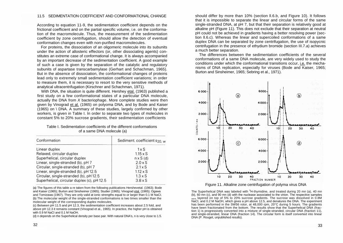
With DNA, the situation is quite different. Hershey etal. (1963) published a first study on a few conformational states of a particular DNA molecule, actually the DNA from X bacteriophage. More complete studies were then given by Vinograd et al. (1965) on polyoma DNA, and by Bode and Kaiser (1965) on \ DNA. A summary of these studies, largely confirmed by other workers, is given in Table I. In order to separate two types of molecules in constant 5% to 20% sucrose gradients, their sedimentation coefficients

Table I. Sedimentation coefficients of the different conformations

of a same DNA molecule (a)

should differ by more than 10% (section ll.6.b, and Figure 10). It follows that it is impossible to separate the linear and circular forms of the same single-stranded DNA, at pH 7, but that their separation is relatively good at alkaline pH (Figure 11). This does not exclude that their separation at neutral pH could not be achieved in gradients having a better resolving power (sec-tion ll.6.c). Whereas the linear and supercoiled conformations of a same duplex DNA can be separated by zone centrifugation, the use of isopycnic centrifugation in the presence of ethydium bromide (section III.7.a) achieves a much better separation.

The differences between the sedimentation coefficients of the several conformations of a same DNA molecule, are very widely used to study the conditions under which the conformational transitions occur, i.e. the mecha-nisms of DNA replication, especially for viruses (Bode and Kaiser, 1965; Burton and Sinsheimer, 1965; Sebring et al., 1971).

(a) The figures of this table a re taken from the following publications Hershevetal. (1963); Bode and Kaiser (1965); Burton and Sinsheimer (1965); Studier (1965); Vinograd etal. (1965); Ogawa and Tomizawa (1967). They are only valid at ionic strengths equal to or larger than 0.1 M NaCI. (b) The molecular weight of the single-stranded conformations is two times smaller than the molecular weight of the corresponding duplex molecules. (c) Between pH 11.5 and pH 12.3, the sedimentation coefficient increases about 2.5 fold, and above pH 12.3 it remains constant (Vinograd et al., 1965). In practice, the higher pH is obtained with 0.9 M NaCI and 0.1 M NaOH. (d) n depends on the Superhelical density per base pair. With natural DNA's, n is very close to 1.5.

32

Figure 11. Alkaline zone centrifugation of polyma virus DNA The Superhelical DNA was labeled with 3H-thymidine, and treated during 20 mn (a), 40 mn (b), 60 mn (c), and 90 mn (d) with the nuclease associated to the virion. The respective samples were layered on top of 5% to 20% sucrose gradients. The sucrose was dissolved in 0.8M NaCI, and 0.2 M NaOH, which gives a pH above 12.5, and denatures the DNA. The experiment has been performed in the SW56 rotor, at 48,000 rpm, 20°C during 5 hours. The gradients have been fractionated from the bottom. The results show that the Superhelical DNA (frac-tion 1) is progressively converted into a mixture of single-stranded, circular DNA (fraction 11), and single-stranded, linear DNA (fraction 14). The circular form is itself converted into linear DNA (P. Rouget, unpublished results).

33

11.6 THE RESOLVING POWER

The analytical applications of zone centrifugation which have been dealt with in the preceding sections - measurement of sedimentation coefficients, measurement of molecular weights, detection of conformational changes -do not necessarily require a complete separation of the respective macro-molecular zones. Most often it does not matter whether two enzyme zones overlap more or less, provided the measurement of the two independent enzymatic activities allows a precise location of the two zones relative to each other (Figure 10). If, instead, zone centrifugation is used to purify one particular macromolecular component, it should be contaminated as little as possible by other components whose sedimentation coefficients are only slightly different. One should then search for the experimental conditions which give an appropriate resolution for each particular case. As will be seen below, one is most often led to find the best compromise between resolving power, the total amount of macromolecules to be purified, and centrifugation time.

We shall first try to analyze the problem of resolution. Unfortunately, an exhaustive analysis will be impossible, since its experimental as well as its theoretical studies are still very uncomplete.

a) General notions As for isopycnic centrifugation (Ifft et al., 1961), the resolving power of zone

centrifugation can be defined as: where ∆ r is the distance which separates two macromolecular zones, and cf2 and ai are the standard deviations of the gaussian curves which both of them describe. In the particular case of zonal rotors. Pollack and Price (1971) propose a slightly different, but experimentally more accessible definition, namely where ∆ V is now the volume by which the two zones are separated, and σν,1 and σν,2 the standard deviations of the volume distribution curves of the zones. (For a given experiment, the two definitions are identical if σ1=σ2; otherwise, Λ and Λv differ only very slightly.) It turns out - and it is obvious a priori - that the resolving power will be the better, the greater the distance between two zones, and the smaller their widths.

The distance - or the volume - which separates two zones is greater, the greater the relative difference between the corresponding sedimentation coefficients. For a given difference, this distance increases with the total

34

distance through which the zones have sedimented, j.a it increases with cen-trifugation time and with the length of the gradient (which depends on the rotor). This distance is smaller in gradients where the sedimentation velocity decreases progressively, than in isokinetic gradients (section II.6.b). The opposite occurs in gradients where the sedimentation velocity increases progressively (Kaempfer and Meselson, 1971).

The width of the zones depends on several factors. As far as the wall effect is negligible (see below), the final zone width always increases with the initial zone width, i.e. with the volume of the initial sample layer. In order to keep the initial zone width close to its theoretical value, one should layer the sample with maximum care (section II.2.d), and avoid any excess of macromolecules (section II.7). In addition, a bad fractionation procedure of the gradient might enlarge the final zone width (section ll.2.f).

Secondly, the final zone width depends on the speed at which the macro-molecules diffuse. As a rule, small molecules diffuse more rapidly than large ones; the former will give rise to broader zones than the latter. Since the broadening of the zones due to diffusion always increases with time, the rotors should always be run at their maximum allowable speed (see sec-tion IIAbforthe particular case of DNA).

The final zone width depends also on the way the sedimentation velocity varies along the gradient. In an isokinetic gradient, the sedimentation velocity will be the same on the front and on the rear of a given zone; in the absence of diffusion, or other perturbing effects, the zone width will remain constant during the whole experiment. If, instead, the sedimentation velocity pro-gressively decreases, the molecules which are at the front of a given zone will sediment slowlier than those which are placed at the rear. A sharpening of the zone will ensue. This gradient induced zone sharpening effect, which was initially described by Schumaker (1966; 1967) and by Berman (1966), was first utilized by Spragg etal. (1969) for their isometric gradients, and was then further developed and applied to hyperbolic and equivolumetric gra-dients by Price and his coworkers (Eikenberry etal., 1970; Pollack and Price, 1971; Price, 1973, a). In addition to the improvment of the resolving power, this sharpening effect has the following advantage; in zonal rotors and iso-kinetic gradients, a macromolecular zone whose diffusion is negligible, is contained in a cylindrical crown of constant thickness but of increasing radius, i.e. the volume occupied by the zone increases progressively and the macromolecules become more and more diluted. If, instead, the shape of the gradient is such that it induces a sharpening of the zones, the dilution is lessened or even inverted. In equivolumetric gradients, non-diffusing zones occupy normally a constant volume.

Gradients in which the sedimentation velocity increases progressively should normally produce a broadening of the zones. But in their CsCI gra-dients, Kaempfer and Meselson (1971) had zones whose final width was the same as in isokinetic gradients. This is probably due to the fact that the expected broadening is much less important than the broadening due to the "wall effect".

35

Λ = ∆ rσ1 + σ2

II-21

Λv =∆ V

σν,1 + σν,2

II-22

The "wall effect" consists of the following: in the cylindrical tubes of the swinging bucket rotors, some molecules hit continuously the walls of the tube along which, then, they tend to slide. This leads to zone broadening (Schumaker, 1967). The existence of the density gradient counteracts the wall effect, but in 5% to 20% sucrose gradients an important broadening still remains. We have observed that in such gradients, zones containing non-diffusing macromolecules suffered a two to three-fold broadening during sedimentation. On the other hand, the fact that the experimental resolving power of macromolecules with a mean molecular weight of 4 x 106

daltons is equal to the theoretical resolving power (Fritsch, 1973, b), suggests that as soon as the diffusion becomes appreciable, the wall effect becomes negligible. It seems also likely that the wall effect becomes less important if one centrifuges less macromolecules, or if one uses a steeper density gradient. One of the main advantages of zonal rotors is that the wall effect does not exist.

The width of zones still increases under several other, but still badly elu-cidated factors. Spragg etal. (1969) speak of "abnormal" broadening, and with Price (1973, a) they seem to relate it to the eventual interactions between the macromolecules and the gradient material (sucrose, etc.). According to Halsall and Schumaker (1970; 1971), and Meuwissen (1973), it should rather be due to the differential diffusion of the macromolecules and the gradient material (section II.7.b).

Finally, it should be remembered that with DNA the final zone width can increase through the fact that the sedimentation coefficient strongly increases with decreasing concentration. It follows that the molecules at the leading edge of the zone will sediment much faster than the molecules placed in the region where their concentration is maximum. Although the rate at which the sedimentation coefficient varies with concentration strongly depends on the molecular weight, DNA concentrations of more than a few fig/ml per zone, induce a significant broadening. At high DNA concentrations, a given zone may occupy one third of the total gradient length. Its shape is no more gaussian, but becomes triangular with a sudden concentration increase at the rear of the zone, and a progressive decrease towards the gradient bottom.

b) Elements for a quantitative study In the recent literature dealing with the resolving power of zone centrifuga-

tion, only part of the preceding elements have been taken into a quantitative study. Nevertheless, several important practical conclusions can be drawn:

- Isokinetic gradients For isokinetic gradients, an equation of the resolving has been derived

under the following assumptions (Fritsch, 1973, a): the gradients are not overloaded with macromolecules, and the wall effect is negligible. The latter assumption is always valid in zonal rotors, and in swinging bucket rotors if the diffusion is relatively important (M<5x106 daltons). The equation is given here under a slightly modified form:

36

Most of the symbols of this equation have already been defined earlier in this chapter, except σo which is the half initial zone width, M, which is a mean of the molecular weight of the two macromolecular species under considera-tion, η, which is the mean viscosity of the sedimentation medium through which the two zones have moved, and r2, which is the distance to the rotor axis of the fastest moving zone.

Equation II-23 confirms that in order to obtain the largest resolving power with a given rotor, it should be used at its maximum speed (see section ll.4.b for the particular case of DNA), that the gradient should be as long as pos-sible (see some optimum filling conditions of the tubes and zonal rotors in Table A.1), and that the fastest sedimenting zone should come as close as possible to the gradient bottom.

With isokinetic sucrose, or glycerol gradients, it turns out that a is almost inversely proportional to the mean viscosity of the gradient. From equation II-23 it then follows that, with a given rotor, the resolving power is nearly the same with all isokinetic gradients, and that it is independent of the temperature.

If the resolving power is proportional to the relative difference between the two sedimentation coefficients, it also depends on the mean molecular weight of the macromolecules under consideration (Figure 12). It should be pointed out that for Mú5x106 daltons, the resolving power is, in principle, independent of the rotor speed and inversely proportional to the initial thick-ness 2 σo of the sample layer. With high molecular weight DNA's (Mú50 x 10s

daltons), it is however necessary to consider the rotor speed effect which has been analyzed by Levin and Hutchinson (1973, a; see also section ll.4.b). Indeed, above a certain rotor speed, two DNA's with very different masses might sediment at the same velocity, and be completely unseparable. On the other hand, with molecular weights smaller than 5x104 daltons, the resolving power is proportional to the rotor speed, and almost independent of 2σo, if the latter is smaller than 5% of the total gradient length.

Equation II-23 allows the comparison of the resolving power of the various rotors (Figure 12 and Table A.1). From Figure 12, it appears that for low molecular weights, appreciable differences exist. It is noteworthy that the rotors with the best resolving power are those which support the less macro-molecular material. For very high molecular weights (M>5x106 daltons), and for 2 σo equal to a constant fraction of the total length, the differences among the rotors almost vanish. Figure 12 and Table A.1 ought to contribute to the choice of the best suited rotor for a given experiment as well as to predict the resolving power upon switching from a low scale to a large scale preparative run.

For the interpretation of Figure 12 and Table A.1, one should also notice

37

Λ =

σ2αω2 +o2 RT

M (1 - νρ) η(r2 - rm)

1/2

(r2 - rm)α 1/2

2

x(s20,w)2 - (s20,w)1

(s20,w)2II-23

that a complete separation of two zones is achieved for A = 3, whereas if A = 2 a slight overlap of the zone occurs; for A = 1.5, the overlap is very appreciable, and almost complete for A = 1 (Ifftetal., 1961; Fritsch, 1973, a, b).

- The sharpening of the zones Every non isokinetic density gradient induces a progressive change of

the zone width. This is because on both sides of the zones the macromolecules sediment at different velocities Berman (1966) has shown that in any gradient, provided the diffusion is negligible and the zones are narrow, the ratio of the final zone width 2 σ to the initial zone width 2o0, is given by:

Figure 12. Resolving power versus molecular weight, for various rotors, and isokinetic gradients

The curves have been drawn from equation II-23, with the assumption that the rotors are spun at their maximum speed, that the filling volumes are those of Table A.1 (Appendix), and that the fastest zone has sedimented to the bottom of the gradient For the calculations it was assumed that the sample volumes were twice as large as those from Table A.1; this is without any influence on Λ in the low molecular weight range, and for high molecular weights it corrects for the "wall effect" (see text). In order to obtain the resolving power in a given rotor, for two macromolecules whose molecular weight is equal to M, the corresponding ordinate is multi-plied by their relative sedimentation coefficient difference, (s1-s2)/s2. a) Rotors SW65, SW56, and SW41; b) Rotor SW50.1; c) Rotors SW50, SW36, and SW27; d) Rotors SW39, and SW25.2; e) Rotors Ti14, and Ti15: f) Rotors AIM, and AI15.

38

f'm/f’ is the measure of an eventual conformational of the macromolecules when they sediment from the distance rm (meniscus) to the distance r. (1-vp)m and (1-vp) are the buoyancy terms, and ηm and η the viscosities of the gradient at rm and r, respectively. The comparison of equations 11-10 and II-24 shows that the ratio 2σ/2σo is actually equal to the ratio of the final velocity to the initial velocity of a given zone.

It follows that every gradient where the final sedimentation velocity of a zone is smaller than its initial sedimentation velocity will induce a sharpening of the zone (Figure 13). On the other hand, if the final velocity is larger than the initial velocity, the zone will broaden.

In zonal rotors, the zone width is usually expressed in volume units, rather than in units of length (equation II-22); the two corresponding sharpening ratios are then related through: From this equation it would seem that in zonal rotors the sharpening is less important than in cylindrical tubes; this is only apparent, since without sharpening (isokinetic gradients), the volume of the zones would increase according to the ratio r/rm, whereas it remains constant in tubes.

No good experimental check of equation II-24 seems to be available. With the tubes of swinging bucket rotors it is particularly difficult, owing to the wall effect. Particularly, in the CsCI gradients of Kaempfer and Meselson (1971), where the sedimentation velocity increases progressively, the total broadening of the zones appears to be identical to the broadening due to the wall effect. In another experiment, where the zone widths of a given DNA have been measured in a 5% to 20%, and in a 5% to 30% sucrose gradients, Piedra and Fritsch (unpublished results) have observed that in the second gradient the zone was 1.4 times narrower than in the first gradient (Figure 14); but in the 5% to 20% gradient the zone was already broadened 2 to 3 times by the wall effect.

In zonal rotors, as well isometric (Spragg et al., 1969), hyperbolic (Eiken-berry, 1970), as equivolumetric gradients (Price, 1973, a) should induce zone sharpening. If such is indeed the case (Price, 1973, a), the sharpening is nevertheless always smaller than expected on the grounds of equations II-24. Sometimes (Spragg et al., 1969), a broadening of the zones occurs. The reasons for these abnormalities are not yet understood, but it could well be that they are simply due to the overload of the gradients with macromolecules (section II.7.b in fine).

If the properties of a gradient are such that they induce some zone sharpening, the two zones will also come closer together than in an isokinetic gradient. The question then arises whether an improvement of the resolving

39

2σ2σo

= f’mf’

(1 - vρ)(1 - vρ)m

ηm

ηrrm

II-24

2σv

2σv, o= 2σ

2σo

rrm

II-24bis

power necessarily follows. The experimental facts presently available, all support the idea that zone sharpening gradients indeed improve the resolu-tion. The equivolumetric gradients have already been mentioned. Similarly, Neal and Florini (1972) could detect seven RNA zones (extracted from chicken liver) in 10% to 70% sucrose gradients (they are necessarily sharp-ening), whereas only four zones could be recognized in 10% to 20% gra-dients. The sharpening gradient used in Figure 13, has also a better resolving power than an isokinetic gradient. On the other hand, not much theoretical

evidence is available yet. It has been shown (Fritsch, unpublished), that in gradients where the sedimentation velocity decreases linearly with distance, the resolution is always larger than in isokinetic gradients. Particularly, if the Ti14 rotor is loaded with a constant 5% to 30% sucrose gradient, the ratio of the final to the initial sedimentation velocity is equal to 0.5, and a 40% increase of the resolution is expected for non-diffusing particles.

Finally, the gradient induced zone sharpening effect also explains the improved resolution of stepwise gradients (Griffith, 1973). The properties of such gradients are still largely unexploited, probably because the centrifuga-tion time is sometimes critical.

Figure 13. Zone centrifugation of polysomes

The polysomes have been extracted from 4 x 102 L5178 y cells, and were layered on a constant 10% to 40% sucrose gradient. The SW25.1 rotor was used at 25,000 rpm, and 5°C; the run length was 4 hours. The centrifuge tube was punctured at the bottom and about 40 fractions of 0.75 ml each were collected. The absorption at 260 nm {• - •{ of each fraction was mea-sured. The zones characterized by sedimentation coefficients of 803, 60S, and 45S corre-spond to whole ribosomes, to the large ribosomal subunit, and to the small subunit, respec-tively. Zones which sediment faster than whole ribosomes, correspond to polysomes of in-creasing size. (From Tiollais etal., 1971.)

The sedimentation velocity (in arbitrary units) of a given macromolecular zone as a function ofthesedimented distance, has also been plotted (---). Its decrease with increasing distance to the rotor axis, shows that this gradient induces a sharpening of the zones. If the experiment had been performed with an isokinetic gradient, the resolution between polysomal zones would not have been as good (Tiollais, personal communication).

Figure 14. Gradient induced zone sharpening of a 5% to 30% constant sucrose gradient

0.2 fig of tritiated \ phage DNA have been layered on two sucrose gradients whose concentra-tion varied linearly from 5% to 20%, and from 5% to 30%, respectively. The gradient volume was 4.8 ml and the sample volume 0.1 ml. Rotor SW50.1 was used at 49,000 rpm and 20°C. The two gradients were spun during 90 mn, and 120 mn, respectively. Under these conditions, it was predicted that both zones would move through approximately 75% of the total gradient length. At the end of the runs the gradients were directly collected into liquid scintillation vials. The radioactivity has been plotted versus the fraction number. Only the interesting region of the gradients has been drawn on the figure.

The measurement of the zone widths at 60% of their height shows that the width in the 5% to 30% gradient (o-o) is 2/1.4 = 1.4 times smaller than the width in the 5% to 20% gradient (•-•). Calculation predicts a 1.5 fold sharpening of the zone (see text).

40 41

1.7 THE MAXIMUM LOAD OF THE GRADIENTS

The use of zone centrifugation as a purification tool of macromolecules or subcellular particules, raises the problem of the total amount of such sub-stances which can be treated in a single run. This is another aspect of zone centrifugation to which much work has been devoted, especially since the appearance of the zonal rotors, and which should be completely understood in the very near future.

The maximum amount of macromolecules which a density gradient can support, is defined as the amount which does not yield more zone broadening than would be expected from the normal sedimentation and diffusion of the macromolecules (and, eventually, from the wall effect). In order to avoid any excessive zone broadening several factors have to be considered. Two of them appear to be relatively well known, namely the hydrostatic stability of the zones, and the differential diffusion between macromolecules and gradient material.

a) The hydrostatic stability of the zones A first, and obvious condition to be satisfied is that the density of the

macromolecular solution to be layered on the gradient be smaller than the density of the gradient just below the initial layer. With gradients whose minimum sucrose concentration is equal to 5%, this means that the concen-tration in the initial sample should always be smaller than 60 mg/ml of proteins, or 30 mg/ml of nucleic acids. But for other reasons (see below) such large concentrations can never be used.

Another condition to be satisfied during the whole sedimentation process is the following: on the leading edge of a zone the macromolecular concen-tration decreases, and to this concentration decrease a density decrease is related (negative density gradient); if this density decrease is compensated through the progressive increase of the density of the sedimentation medium (positive density gradient), i.e. if the overall density always increases in the direction of the centrifugal field (positive resultant density gradient), the macromolecular zone will be stable. If the resultant density gradient were negative, the zone would broaden until the negative gradient could be com-pensated by the positive one. One understands immediately that this stability criterion depends on the amount of macromolecules contained in a given zone (Figure!).

If stated in the preceding terms, the problem of the maximum load of the gradients has been treated by several authors (Svensson etal., 1957; Berman, 1966; Vinograd and Bruner, 1966; Schumaker, 1967) who derived the fol-lowing equation:

where Qmax. is the total amount of macromolecules to be supported by a zone of thickness 20 and whose area is equal to A; dρ/dr is the supporting

42

density gradient in the zone. If the sample is layered as an inverted gradient (section II.2.c and II.7.b), 2tf designates the whole sample thickness; in this particular case the second member of equation II-25 can be multiplied by 2 (Svensson etal., 1957; Eikenberry etal., 1970; Meuwissen and Heirwegh, 1970). If the diffusion of the macromolecules to be centrifuged is appreciable the Qmax. values given by equation II-25 can as well be multiplied by 2 (Vino-grad and Bruner, 1966). It is with the latter assumption that the Qmax. values of Table A.1 have been calculated.

None of the parameters of the preceding equation is necessarily constant during centrifugation. In the zonal rotors, A = 2Tihr (h is the height of the rotor) and increases progressively during sedimentation; in the swinging bucket rotors instead, A is constant and equal to the cross-sectional area of the tubes. It is essentially because A varies very much from one rotor to another that their capacities are very different. The zone thickness depends on the following factors: the initial width of the sample layer; the diffusion of the macromolecules, which always leads to a broadening of the zones; the wall effect; the shape of the gradient, which might induce either a sharp-ening or a broadening of the zones (section II.6.b). For a given experiment, Qmax. should always be calculated for the conditions where A (2σ)2 dρ/dr is minimum.

With 5% to 20% isokinetic sucrose gradients this product is always the smallest at the beginning of an experiment. Hence Qmax. should be calculated for the initial thickness of the sample layer, and, for zonal rotors, with the initial value of A, taking r = rm. The Qmax. values of Table A.1 have been calculated in this way; they correspond to 5% to 20% constant sucrose and to 2cr0 equal to 2.5% of the length of the gradient. With constant 10% to 30% glycerol the figures of Table A.1 should be reduced by 20%. With both these gradients the maximum load of nucleic acids is equal to 60% of the protein load.

The comparison of the Λrel and Qmax values of Table A.1 shows that the rotors which have the best resolving power are those which support the smallest amount of macromolecules.

If one should resort to 5% to 40% sucrose gradients in order to improve the resolving power, the gradient would induce a zone sharpening equal to (2σ/2σo), and Qmax. should be calculated for a zone width equal to 2<j0 (2a/2a0). With the Ti14 zonal rotor, one would expect (2a/2a0) = 0.36, and the load would be equal to (0.36)2 = 0.13 times the load of a 5% to 20% gradient. But since the gradient dp/dr would be two times larger, one finally ends up with a load 4 times smaller than with the 5% to 20% gradient. This calcula-tion does not include the progressive increase of the gradient area A. But nevertheless, this is another example which illustrates how one is often led to find the best compromise between macromolecular load and resolving power.

Berman (1966) has calculated that in zonal rotors a zone which is initially stable remains stable during its sedimentation, if the density gradient has a hyperbolic shape (equation II-5 of section ll.2.c): the progressive decrease

43

Qmax = A(2σ)2 dρ/dr2 (1 - vρ)

II-25

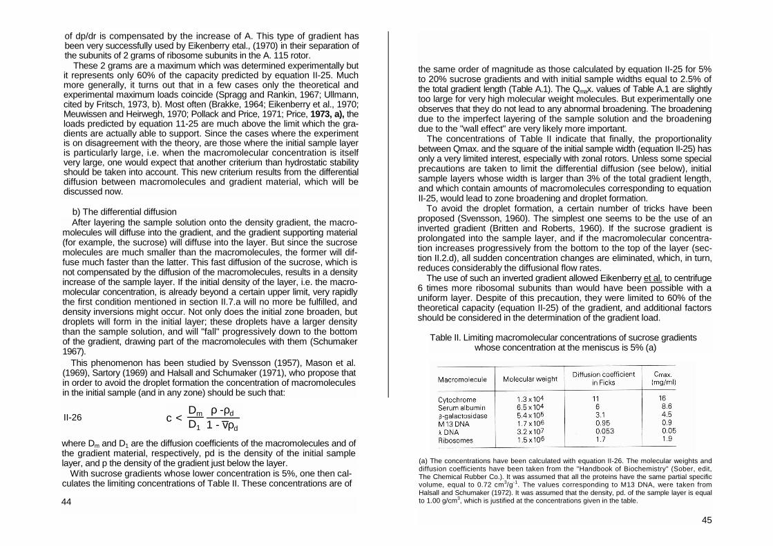
of dp/dr is compensated by the increase of A. This type of gradient has been very successfully used by Eikenberry etal., (1970) in their separation of the subunits of 2 grams of ribosome subunits in the A. 115 rotor.

These 2 grams are a maximum which was determined experimentally but it represents only 60% of the capacity predicted by equation II-25. Much more generally, it turns out that in a few cases only the theoretical and experimental maximum loads coincide (Spragg and Rankin, 1967; Ullmann, cited by Fritsch, 1973, b). Most often (Brakke, 1964; Eikenberry et al., 1970; Meuwissen and Heirwegh, 1970; Pollack and Price, 1971; Price, 1973, a), the loads predicted by equation 11-25 are much above the limit which the gra-dients are actually able to support. Since the cases where the experiment is on disagreement with the theory, are those where the initial sample layer is particularly large, i.e. when the macromolecular concentration is itself very large, one would expect that another criterium than hydrostatic stability should be taken into account. This new criterium results from the differential diffusion between macromolecules and gradient material, which will be discussed now.

b) The differential diffusion After layering the sample solution onto the density gradient, the macro-

molecules will diffuse into the gradient, and the gradient supporting material (for example, the sucrose) will diffuse into the layer. But since the sucrose molecules are much smaller than the macromolecules, the former will dif-fuse much faster than the latter. This fast diffusion of the sucrose, which is not compensated by the diffusion of the macromolecules, results in a density increase of the sample layer. If the initial density of the layer, i.e. the macro-molecular concentration, is already beyond a certain upper limit, very rapidly the first condition mentioned in section II.7.a will no more be fulfilled, and density inversions might occur. Not only does the initial zone broaden, but droplets will form in the initial layer; these droplets have a larger density than the sample solution, and will "fall" progressively down to the bottom of the gradient, drawing part of the macromolecules with them (Schumaker 1967).

This phenomenon has been studied by Svensson (1957), Mason et al. (1969), Sartory (1969) and Halsall and Schumaker (1971), who propose that in order to avoid the droplet formation the concentration of macromolecules in the initial sample (and in any zone) should be such that:

the same order of magnitude as those calculated by equation II-25 for 5% to 20% sucrose gradients and with initial sample widths equal to 2.5% of the total gradient length (Table A.1). The Qmax. values of Table A.1 are slightly too large for very high molecular weight molecules. But experimentally one observes that they do not lead to any abnormal broadening. The broadening due to the imperfect layering of the sample solution and the broadening due to the "wall effect" are very likely more important.

The concentrations of Table II indicate that finally, the proportionality between Qmax. and the square of the initial sample width (equation II-25) has only a very limited interest, especially with zonal rotors. Unless some special precautions are taken to limit the differential diffusion (see below), initial sample layers whose width is larger than 3% of the total gradient length, and which contain amounts of macromolecules corresponding to equation II-25, would lead to zone broadening and droplet formation.

To avoid the droplet formation, a certain number of tricks have been proposed (Svensson, 1960). The simplest one seems to be the use of an inverted gradient (Britten and Roberts, 1960). If the sucrose gradient is prolongated into the sample layer, and if the macromolecular concentra-tion increases progressively from the bottom to the top of the layer (sec-tion II.2.d), all sudden concentration changes are eliminated, which, in turn, reduces considerably the diffusional flow rates.

The use of such an inverted gradient allowed Eikenberry et al. to centrifuge 6 times more ribosomal subunits than would have been possible with a uniform layer. Despite of this precaution, they were limited to 60% of the theoretical capacity (equation II-25) of the gradient, and additional factors should be considered in the determination of the gradient load.

Table II. Limiting macromolecular concentrations of sucrose gradients

whose concentration at the meniscus is 5% (a)

where Dm and D1 are the diffusion coefficients of the macromolecules and of the gradient material, respectively, pd is the density of the initial sample layer, and p the density of the gradient just below the layer.

With sucrose gradients whose lower concentration is 5%, one then cal-culates the limiting concentrations of Table II. These concentrations are of

44

(a) The concentrations have been calculated with equation II-26. The molecular weights and diffusion coefficients have been taken from the "Handbook of Biochemistry" (Sober, edit, The Chemical Rubber Co.). It was assumed that all the proteins have the same partial specific volume, equal to 0.72 cm3/g-1. The values corresponding to M13 DNA, were taken from Halsall and Schumaker (1972). It was assumed that the density, pd. of the sample layer is equal to 1.00 g/cm3, which is justified at the concentrations given in the table.

45

c <DmD1

ρ -ρd

1 - vρdII-26

Hence, Meuwissen (1973) was led to consider the problem from the point of view of the conservation of the volume fluxes. In a macromolecular zone this statement is explicited according to the following equation:

where the subscripts m and 1 are relative to the macromolecules and to the gradient material, respectively; c are the concentrations, and D the diffusion coefficients. The (-) sign is due to the fact that at the leading edge of a zone the gradient material and macromolecular density gradients are of opposite signs.

Both the Halsall and Schumaker approach, and the Meuwissen approach, set an upper limit to the concentration of macromolecules. This is different from the hydrostatic stability criterium, according to which the concentra-tion could be increased (indefinitely?) provided the zone width was increased correspondingly. Both approaches also state that the limiting concentration is proportional to the ratio of the diffusion coefficients of the macromolecules and gradient material.

But with equation II-28, Meuwissen finds limiting concentrations about 10 times smaller than those determined from the Halsall and Schumaker equation. On the other hand, the Meuwissen approach has the considerable advantage to explain why the load of a gradient is much smaller at rest than upon centrifugation (Brakke, cited by Schumaker, 1967, Nasonetal.,1969). Nevertheless, the limiting concentrations calculated according to the equa-tion of Halsall and Schumaker (Table II) are much closer to those which are experimentally observed; in particular, the limiting concentration of 2 mg/ml of ribosomes has been reported by Price (1973, a).

The introduction of the sedimentation fluxes in equation II-28 does not resolve the contradiction between the two theories, since as pointed out by Meuwissen (1973) himself "all practical density gradient procedures in use so far have to go through at least two cycles where the external centrifugal force field causing effective migration of the components is quasi absent."

Although the quantitative and experimental aspects of differential diffu-sion have still to be worked out further, it explains some older observations of Meuwissen and Heirwegh (1970), namely that the load of a gradient can be increased if the molecular weight of the gradient supporting material is itself increased (large molecules diffuse less than small ones), and that the load of the gradients is not indefinitely proportional to dp/dr.

Price (1973, a), on the contrary, attributes the preceding molecular weight effect to the interactions of the gradient material with the macromolecules. The eventual existence of such interactions is corroborated by the slight difference between the sedimentation coefficients measured by zone cen-trifugation and by analytical boundary sedimentation where the concentra-tion of the secondary solute (sucrose, NaCI, etc.) is usually extremely small (see section II.3.a). It seems likely that at high macromolecular concentra-

46

tions the local decrease of the sucrose and water concentrations changes as well the hydrostatic stability criterium, the conditions of the differential diffusion, as the interactions between macromolecules and gradient mate-rial. But nothing very precise is yet available on the manner in which these various factors could affect the macromolecular zones.

c) The particular case of DNA Neither the hydrostatic stability criterion, nor the differential diffusion ef-

fect should be used in determining the maximum DNA load, but the fact that the sedimentation coefficients very strongly increases with decreasing DNA concentration. In order to avoid an excessive broadening of the zones, and in order to maintain the meaning of the expression "zone" centrifuga-tion, one should keep the DNA concentrations below 10 jig/ml per zone for molecular weights smaller than 20x106 daltons. For larger molecular weights the concentration should be decreased correspondingly. Unfortunatelly, no systematic study of this problem has yet been undertaken.

d) How to centrifuge a given amount of macromolecules Obviously, no general answer can be given to this problem. This is not

only because our knowledge of the various elements on which the maximum load of the gradient depends on is still incomplete (see above), but still other factors, particular to each experiment, have to be considered. In each particular case, a minimum resolving power will have to be achieved, which will depend on the factors discussed in section 11-6, but also on the par-ticular mixture of macromolecules, or particles, to be centrifuged. For the centrifugation of low molecular weight macromolecules, whose diffusion is relatively important, the centrifugation time will have to be shortened as much as possible. The single methods of measuring sedimentation coef-ficients will require the use of particularly shaped gradients (section II.3.c).

First of all, the amount of macromolecules to be loaded on a given gra-dient should always be below the limits determined from both the hydrostatic stability criterion and the differential diffusion effect. Examples where the former gives larger limiting concentrations than the latter have already been mentioned. But with low molecular weight macromolecules (Table I), and/or with high molecular weight gradient material, the differential diffusion ef-fect allows relatively large concentrations; if the hydrostatic stability criterion were no longer satisfied, the zones would nevertheless be unstable.

In so far as the properties (resolving power, and gradient load) of the rotors given in Figure 12 and Table A.1 are appropriate to a given experi-ment, it is advantageous indeed to use constant 5% of 20% sucrose gra-dients. In addition to their isokinetic character, they are easy to set up, their resolving power is reasonably good, and the centrifugation times are the shortest. In zonal rotors, they might give an up to two- fold dilution of the sample; if this were excessive, an equivolumetric gradient should be favored. With swinging bucket rotors, the simultaneous use of six gradients should be considered.

47

dcmdc1

>v1vm

DmD1

-II-28

In case where, for a given rotor, the maximum loads of Tables II and A.1 are too low, three factors can be changed: the volume of the initial sample layer, the use of an inverted gradient for the layering, and the properties of the gradient. With very large loads, a more or less important loss of resolu-tion unavoidably ensues. This appears very clearly from a comparison of the results of Eikenberry etal. (1970) and Pollack and Price (1971), on the separa-tion of ribosomal subunits.

If the resolving power of the 5% to 20% sucrose gradients were insuf-ficient, 5% to 40% gradients seem to be a good recourse. But their zone sharp-ening effect (increase of the concentration) should be taken into account. With a crude cellular extract, or a mixture of macromolecules with a wide sedimentation heterogeneity, the disadvantages of this effect will be largely compensated by the separation of the individual components into different zones.

Finally, in many cases, only the experiments will allow to find out the best suited conditions for the centrifugation of very large amounts of macro-molecules. Preliminary experiments at a low scale should be helpful.

48

CHAPTER III

Isopycnic centrifugation

III.1 THE PRINCIPLE OF THE METHOD

Isopycnic centrifugation designates density gradient centrifugation methods, where the macromolecules end up in a position where their apparent density -or, buoyant density - is equal to the local density of the gradient. Above this position, the apparent buoyancy term of the macromolecules (section ll.S.a) is positive, and they sediment in the direction of the centrifugal force field, whereas below this position (1-vp)app is negative, and the macromolecules move in the opposite direction. Macromolecules with different buoyant densities distribute themselves into bands which occupy different positions in the gradient. Thus, isopycnic centrifugation separates macromolecules according to their relative buoyant density differences, and no longer ac-cording to their sedimentation coefficients, as in zone centrifugation.

For isopycnic centrifugation, the density gradients can be set up, either preliminary to the centrifugation, or they establish themselves upon the influence of the centrifugal force field.

In the first case, gradients are prepared as for zone centrifugation, except that for a given kind of macromolecules, the gradient material is used at much higher concentrations. Most continuous flow centrifugations enter into this category, and examples will be given in section III.7.

For reasons which will appear below, the method which uses gradients which establish themselves during centrifugation is still called equilibrium isopycnic centrifugation. Because of its own methodology, its very wide use, and its numerous applications, the present chapter will be almost completely devoted to the equilibrium method.

Initially designed for the analytical centrifuge (Meselson etal.. 1957), this method has been very rapidly used with the preparative centrifuges and swinging bucket rotors (Weigle et al., 1959), and then with the zonal rotors (El Aaser etal., 1966: Whitson etal., 1966).

Its principle is the following: centrifugation of a concentrated salt solu-tion - cesium chloride, for example - leads to a difference in salt concentra-tion between the two ends of the liquid column; to this concentration variation corresponds a density variation, or density gradient. After a certain time of centrifugation, this density gradient reaches an equilibrium state, where the

49