WORCESTER POLYTECHNIC INSTITUTE

Preparation and Characterization of Composite PES/Nanoparticle

Membranes A Major Qualifying Project submitted to the faculty of Worcester Polytechnic Institute in partial

fulfillment of the requirements for the Degree of Bachelor of Science in Environmental Engineering

Submitted by Patrick Sheppard

4/25/2013

Submitted to:

Project Advisor: Professor DiBiasio, Worcester Polytechnic Institute

Project Advisor: Professor Chi, Shanghai Jiao Tong University

Abstract

Membrane fouling remains an obstacle to widespread adoption of membrane technologies, and improving the hydrophilicity of a membrane’s surface reduces membrane fouling. Therefore, there has been significant interest in improving membrane hydrophilicity. Many researchers have accomplished this by imbedding inorganic nanoparticles, often metal oxides, on polymeric membrane surfaces. These studies show that antifouling performance is significantly improved after the addition of inorganic nanoparticles. However, despite this multitude of studies that demonstrate the effectiveness of this technique, no study has critically analyzed which nanoparticle is most effective at reducing fouling. This study helps to fill this research gap. Four different nanoparticles TiO2, SiO2, ZnO, and ZrO2, were dispersed in a polyethersulfone (PES) casting solution at 1 wt %, and composite membranes were then prepared from this casting solution via the phase inversion method. The resulting membranes’ properties were characterized, and the results were compared. Of the four particles tested, SiO2 displayed the best antifouling performance.

1 | P a g e

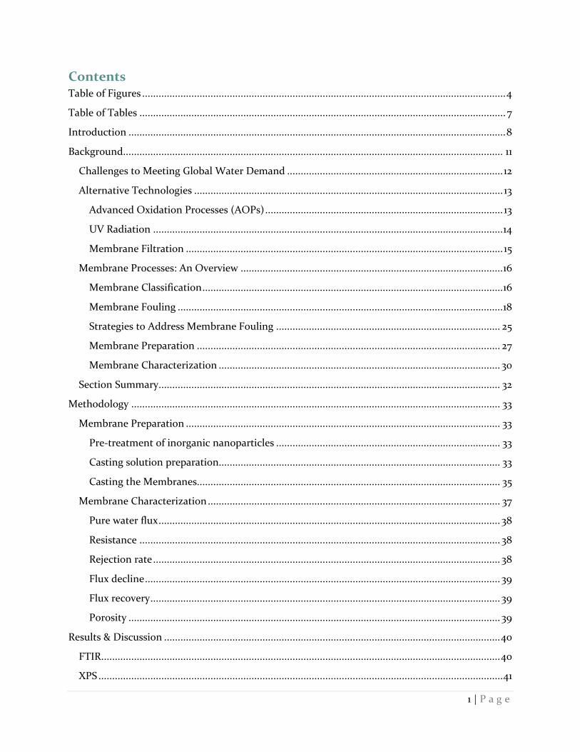
Contents Table of Figures ..................................................................................................................................... 4

Table of Tables ...................................................................................................................................... 7

Introduction .......................................................................................................................................... 8

Background ........................................................................................................................................... 11

Challenges to Meeting Global Water Demand ............................................................................... 12

Alternative Technologies ................................................................................................................. 13

Advanced Oxidation Processes (AOPs) ....................................................................................... 13

UV Radiation ................................................................................................................................ 14

Membrane Filtration .................................................................................................................... 15

Membrane Processes: An Overview ................................................................................................ 16

Membrane Classification .............................................................................................................. 16

Membrane Fouling ....................................................................................................................... 18

Strategies to Address Membrane Fouling .................................................................................. 25

Membrane Preparation ............................................................................................................... 27

Membrane Characterization ....................................................................................................... 30

Section Summary ............................................................................................................................. 32

Methodology ....................................................................................................................................... 33

Membrane Preparation ................................................................................................................... 33

Pre-treatment of inorganic nanoparticles .................................................................................. 33

Casting solution preparation....................................................................................................... 33

Casting the Membranes............................................................................................................... 35

Membrane Characterization ........................................................................................................... 37

Pure water flux ............................................................................................................................. 38

Resistance .................................................................................................................................... 38

Rejection rate ............................................................................................................................... 38

Flux decline .................................................................................................................................. 39

Flux recovery ................................................................................................................................ 39

Porosity ........................................................................................................................................ 39

Results & Discussion ........................................................................................................................... 40

FTIR .................................................................................................................................................. 40

XPS .................................................................................................................................................... 41

2 | P a g e

ZrO2 ............................................................................................................................................. 43

Hydrophilicity.................................................................................................................................. 44

Contact Angle .............................................................................................................................. 44

Antifouling Performance ................................................................................................................. 46

Summary of Membrane Antifouling Performance ..................................................................... 50

Pure Water Flux ............................................................................................................................... 50

Rejection Rate ................................................................................................................................... 51

Porosity ............................................................................................................................................ 52

Roughness ........................................................................................................................................ 53

Mechanical Properties ..................................................................................................................... 54

Thermal Properties .......................................................................................................................... 56

SEM ...................................................................................................................................................... 57

Cross Section ................................................................................................................................ 57

Bottom Surface ............................................................................................................................ 59

Summary .......................................................................................................................................... 59

Recommendations................................................................................................................................ 61

Treatment Facility Design................................................................................................................... 62

Introduction: Membrane Bioreactor .............................................................................................. 62

Cost Comparison: Pure PES Membrane versus SiO2 Modified Membrane .................................. 63

Excess Sludge ................................................................................................................................... 65

Oxygen Demand .............................................................................................................................. 66

Capital Costs .................................................................................................................................... 67

Summary .......................................................................................................................................... 68

References ............................................................................................................................................ 69

Appendix 1: Information on Methodology ......................................................................................... 73

Appendix 2: Raw Data ......................................................................................................................... 74

Contact Angle Data ......................................................................................................................... 74

Pure Water Flux Data ...................................................................................................................... 74

Flux Recovery Data .......................................................................................................................... 75

Porosity ............................................................................................................................................ 76

Viscosity ........................................................................................................................................... 77

Mechanical Properties ..................................................................................................................... 79

3 | P a g e

Breaking Force ............................................................................................................................. 79

Elongation Rate ........................................................................................................................... 79

Appendix 3: Calibration Curves .......................................................................................................... 80

4 | P a g e

Table of Figures Figure 1: Projected global water scarcity by 2025 ................................................................................ 11

Figure 2: An example of an advanced oxidation process with Hydrogen Peroxide (Sewerage

Business Management Centre) ............................................................................................................ 13

Figure 3: Impact of UV radiation on DNA. Demonstrates how UV radiation inactivates pathogens

(DaRo UV) ............................................................................................................................................ 15

Figure 4: Illustration of a membrane process (Saddatt, 2011) ............................................................. 16

Figure 5: Illustration of the four major classifications of membranes based on permeate particle

size, MF, UF, NF, and RO, as well as some of the sizes of many common pollutants (Davis and

Masten, 2009). ...................................................................................................................................... 17

Figure 6: The three phases of fouling. In the first phase, which lasts roughly one minute, flux loss

is primarily caused by concentration polarization. In the second phase, which lasts between one

and three hours, the flux declines at a moderate rate due to protein deposition on the membrane

surface. And in the final phase, which continues indefinitely, the flux declines slowly due to

further protein deposition. .................................................................................................................. 19

Figure 7: Illustration of concentration polarization, which leads to the first phase of flux loss

during membrane filtration. ................................................................................................................ 19

Figure 8: Illustration of the electrical double layer that forms around charged particles

(http://www.substech.com/dokuwiki/lib/exe/fetch.php?w=&h=&cache=cache&media=electric_do

uble_layer.png) .................................................................................................................................... 20

Figure 9: Graphical representation of the DLVO Theory

(http://www.malvern.com/labeng/industry/colloids/dlvo_theory_1.jpg) ......................................... 21

Figure 10: Illustration of hydrophobic interactions among components in water. These

hydrophobic interactions increase contact between hydrophobic membrane surfaces and

hydrophobic foulants in wastewater which leads to increased fouling.

(http://chemwiki.ucdavis.edu/Physical_Chemistry/Physical_Properties_of_Matter/Intermolecular

_Forces/Hydrophobic_interactions) .................................................................................................. 22

Figure 11: Demonstrates two different types of membrane strucutres, symmetric and asymmetric.

(a) is symmetric, as the pores are all nearly equal in size. (b) is asymmetric, as it consists of two

distinct layers (Membrane Structure). ............................................................................................... 28

Figure 12: Schematic representation of three dry-wet separation processes. A) precipitation with

nonsolvent vapor; B) evaporation of solvent; C) immersion precipitation. The arrows denote the

net direction of diffusion for each step. Polymer, solvent, and nonsolvent are represented by P, S,

and NS, respectively (Kools and Catherina, 1998). ............................................................................ 29

Figure 13: Ternary phase diagram for the phase inversion process through immersion precipitation

(Matar, Hewitt and Ortiz, 1989) ......................................................................................................... 30

Figure 14: Illustration of contact angle (http://en.wikipedia.org/wiki/File:Contact_angle.svg) ..... 32

Figure 15: Weight percentages of the components of the pure PES membrane ............................... 34

Figure 16: Weight percentages of the components of the four modified PES membranes .............. 34

Figure 17: Three of the completed casting solutions .......................................................................... 35

Figure 18: The glass plates that the casting solutions are poured onto ............................................ 36

5 | P a g e

Figure 19: This machine evenly distributes the casting solutions across the glass plates at a

specified thickness .............................................................................................................................. 37

Figure 20: Fourier transform infrared spectroscopy results. The different peaks correspond to

different organic functional groups. Each colored line corresponds to a different membrane. ...... 40

Figure 21: Summary of XPS data for all five membranes .................................................................... 41

Figure 22: Comparison of the XPS results for the SiO2 modified membrane and the pure PES

membrane. The red lines correspond to the data for the SiO2 membrane, and the blue lines

correspond to the data for the pure PES membranes. As is clear, each membrane contained

oxygen, carbon, nitrogen, and sulfur. However, only the SiO2 modified membrane contained

silicon, as expected. ............................................................................................................................. 42

Figure 23: Comparison of the XPS results for the TiO2 modified membrane and the pure PES

membrane. The red lines correspond to the data for the TiO2 membrane, and the gold lines

correspond to the data for the pure PES membranes. As is clear, each membrane contained

oxygen, carbon, nitrogen, and sulfur. However, only the TiO2 modified membrane contained

titanium, as expected. ......................................................................................................................... 42

Figure 24: Comparison of the XPS results for the ZnO modified membrane and the pure PES

membrane. The red lines correspond to the data for the ZnO membrane, and the blue lines

correspond to the data for the pure PES membranes. As is clear, each membrane contained

oxygen, carbon, nitrogen, and sulfur. However, only the ZnO modified membrane contained zinc,

as expected. ......................................................................................................................................... 43

Figure 25: Comparison of the XPS results for the ZnO modified membrane and the pure PES

membrane. The red lines correspond to the data for the ZnO membrane, and the purple lines

correspond to the data for the pure PES membranes. As is clear, each membrane contained

oxygen, carbon, nitrogen, and sulfur. However, only the ZrO2 modified membrane contained

zirconium, as expected........................................................................................................................ 43

Figure 26: This image shows amorphous SiO2 and water molecules. Because both are polar, the

two attract each other. The silicon image was taken from

http://upload.wikimedia.org/wikipedia/commons/8/8b/SiO2.svg. The water molecule image was

taken from http://image.tutorvista.com/cms/images/44/molecular-geometry-of-water.JPG. ....... 44

Figure 27: Contact angles of each of the prepared membranes. PES had the largest contact angle

followed by ZrO2, SiO2, TiO2, and ZnO. ........................................................................................... 45

Figure 28: Reduction in the contact angle of the four modified membranes as compared to the

pure PES membrane. The ZnO membrane showed the greatest contact angle reduction, followed

by TiO2, SiO2, and then ZrO2. ........................................................................................................... 46

Figure 29: Flux decline curves for all five prepared membranes. On the x-axis is flux (L/m2*hr),

and on the x-axis is the time when the flux measurement was taken (minutes). The longer it takes

for the graph to plateau, the better the antifouling performance..................................................... 47

Figure 30: Illustrates the amount of time it took each membrane to reach a constant flux. The

pure PES membrane took the shortest amount of time, followed by ZnO, ZrO2, and then SiO2

and TiO2. ............................................................................................................................................. 48

Figure 31: % of initial pure water flux recovered after the membranes were cleaned with pure

water. ZnO showed the greatest original flux recovery followed by SiO2, TiO2, ZrO2, and PES ... 49

6 | P a g e

Figure 32: Percent improvement in flux after cleaning with pure water of all five prepared

membranes .......................................................................................................................................... 50

Figure 33: Initial pure water flux prior to filtration with the BSA wastewater. ................................. 51

Figure 34: Rejection rate of all five prepared membranes ................................................................. 52

Figure 35: Porosity of all five prepared membranes ........................................................................... 53

Figure 36: Roughness values for all five prepared membranes ......................................................... 54

Figure 37: Elongation rate of the five prepared membranes ............................................................. 55

Figure 38: Breaking force of the five prepared membranes ............................................................... 56

Figure 39: Glass transition temperatures of the five prepared membranes. ..................................... 57

Figure 40: Cross sectional SEM image of the five prepared membranes at a scale of 100

micrometers......................................................................................................................................... 58

Figure 41: Bottom surface SEM image of the five prepared membranes at a scale of 10 micrometers

.............................................................................................................................................................. 59

Figure 42: Schemactic of typical CAS and MBR systems

(http://upload.wikimedia.org/wikipedia/en/thumb/c/c0/MBRvsASP_Schematic.jpg/550px-

MBRvsASP_Schematic.jpg) ................................................................................................................. 62

Figure 43: BSA calibration curve, which was generated using the data in ....................................... 80

7 | P a g e

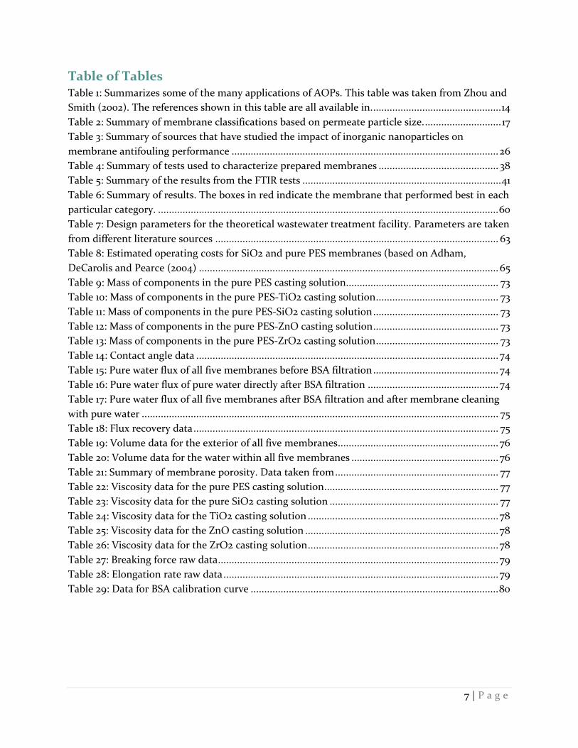
Table of Tables Table 1: Summarizes some of the many applications of AOPs. This table was taken from Zhou and

Smith (2002). The references shown in this table are all available in. ............................................... 14

Table 2: Summary of membrane classifications based on permeate particle size. ............................ 17

Table 3: Summary of sources that have studied the impact of inorganic nanoparticles on

membrane antifouling performance .................................................................................................. 26

Table 4: Summary of tests used to characterize prepared membranes ............................................ 38

Table 5: Summary of the results from the FTIR tests ......................................................................... 41

Table 6: Summary of results. The boxes in red indicate the membrane that performed best in each

particular category. ............................................................................................................................. 60

Table 7: Design parameters for the theoretical wastewater treatment facility. Parameters are taken

from different literature sources ........................................................................................................ 63

Table 8: Estimated operating costs for SiO2 and pure PES membranes (based on Adham,

DeCarolis and Pearce (2004) .............................................................................................................. 65

Table 9: Mass of components in the pure PES casting solution........................................................ 73

Table 10: Mass of components in the pure PES-TiO2 casting solution ............................................. 73

Table 11: Mass of components in the pure PES-SiO2 casting solution .............................................. 73

Table 12: Mass of components in the pure PES-ZnO casting solution .............................................. 73

Table 13: Mass of components in the pure PES-ZrO2 casting solution ............................................. 73

Table 14: Contact angle data ............................................................................................................... 74

Table 15: Pure water flux of all five membranes before BSA filtration .............................................. 74

Table 16: Pure water flux of pure water directly after BSA filtration ................................................ 74

Table 17: Pure water flux of all five membranes after BSA filtration and after membrane cleaning

with pure water ................................................................................................................................... 75

Table 18: Flux recovery data ................................................................................................................ 75

Table 19: Volume data for the exterior of all five membranes ........................................................... 76

Table 20: Volume data for the water within all five membranes ...................................................... 76

Table 21: Summary of membrane porosity. Data taken from ............................................................ 77

Table 22: Viscosity data for the pure PES casting solution ................................................................ 77

Table 23: Viscosity data for the pure SiO2 casting solution .............................................................. 77

Table 24: Viscosity data for the TiO2 casting solution ...................................................................... 78

Table 25: Viscosity data for the ZnO casting solution ....................................................................... 78

Table 26: Viscosity data for the ZrO2 casting solution ...................................................................... 78

Table 27: Breaking force raw data ....................................................................................................... 79

Table 28: Elongation rate raw data ..................................................................................................... 79

Table 29: Data for BSA calibration curve ........................................................................................... 80

8 | P a g e

Introduction According to the World Health Organization (2009), water scarcity is a growing issue that affects

one in three people on every continent. Population growth, urbanization, increased standards of

living, and the expansion of industrial activities are exacerbating this issue (Choi et al., 2002).

Therefore, there is a growing need for better water resource management, which includes more

effective water and wastewater treatment technologies. Of these technologies, membrane

treatment is particularly promising. Zhou and Smith (2002) explain that membrane processes

offer several advantages over conventional treatment processes: they are able to produce high

quality effluent for a diverse range of inputs, do not require chemical addition under most

circumstances, reduce the amount of solids disposal, occupy a small amount of space, are easy to

control, and reduce operation and maintenance costs.

However, membrane fouling remains an obstacle to widespread adoption of membrane

technologies (Meng et al., 2009). Huang et al. (2012) explain that membrane fouling is caused by

the deposition of pollutants on the membrane surface or from adsorption of pollutants into

membrane pores. It leads to reduced flux and therefore increased energy usage over time. It also

often creates the need for chemical cleaning, which further increases cost and maintenance

requirements (Huang et al., 2012).

Currently, organic polymers are the most commonly used materials for commercial membranes

(Zhou and Smith, 2002). However, organic polymers have a hydrophobic surface which, as

observed in many studies, makes them particularly susceptible to membrane fouling (Su et al.,

2011; Yu et al., 2005; Choi et al., 2002). Fouling is more severe in hydrophobic membranes because

of hydrophobic interactions between solutes, microbial cells, and membrane material (Choi et al.,

2002).

As a result, there has been significant interest recently in discovering ways to improve the

hydrophilicity of organic polymer membranes (Shen et al., 2011). Wu et al. (2008) explain that

several methods have been employed to modify membrane surfaces to make them more

hydrophilic, including the application of ultraviolet radiation, blending with hydrophilic

materials, graft polymerization, and plasma grafting. Of these methods, blending with hydrophilic

materials, particularly inorganic nanoparticles, has attracted the most attention because it

requires mild synthesis conditions during membrane preparation (Genne, Kuypers and Leysen,

1996).

Li et al. (2008) write that there are three methods commonly used to blend inorganic materials

with polymer membranes: (1) disperse nanoparticles in the casting solution directly and prepare

the composite membranes via phase inversion; (2) add prepared sol containing nanoparticles in

the casting solution and prepare the composite membranes via phase inversion; and (3), dip the

prepared membrane in an aqueous suspension containing nanoparticles and prepare the

composite membranes via self-assembly. Several studies have applied these methods to blend

different nanoparticles with organic polymer membranes. The nanoparticles used include TiO2 (Li

et al., 2009; Wu et al., 2008) SiO2 (Huang et al., 2012; Shen et al., 2011), ZrO2 (Maximous et al.,

9 | P a g e

2010; Bottino, Capannelli and Comite, 2002; Genne, Kuyperes and Leysen, 1996), and ZnO (Shen

et al., 2012).

Of these nanoparticles, TiO2 has been studied the most thoroughly due to its stability, availability,

(Wu et al., 2008) high hydrophilicity, and photocatalytic potential (Li et al., 2009). Jing-Feng Li et

al. (2009) dispersed varying concentrations of TiO2 nanoparticles (0-5 wt %) in polyethersulfone

(PES) casting solutions and prepared composite membranes via phase inversion. They found that

the composite membranes had enhanced thermal stability, hydrophilicity, and permeation

performance. They recommended an optimal loading rate of 1-2 wt % TiO2. Wu et al. (2008) also

prepared TiO2/PES composite membranes via nanoparticle dispersion and phase inversion. They

confirmed Jing-Feng Li et al.’s findings that the addition of TiO2 enhanced the hydrophilicity,

thermal stability, and mechanical strength of the membrane. However, they recommended an

optimal TiO2 loading rate of 0.5 wt % rather than 1-2 wt %. Jian-Hua Li et al. (2008) modified poly

(styrene-alt-maleic anhydride)/poly(vinylidene fluoride) (SMA/PVDF) to contain TiO2

nanoparticles via the self-assembly method. They also confirmed that the modified membranes

had enhanced hydrophilicity and superior permeability.

SiO2, though not as widely studied as TiO2, has also been analyzed. Shen et al. (2011) prepared

PES/SiO2 composite membranes (0-5 wt % SiO2) by the phase inversion method. They found that

pure and raw water flux increased, hydrophilicity was enhanced, and anti-fouling ability increased

with the addition of SiO2. Huang et al. (2012) prepared mesoporous silica (MS) modified PES

membranes via phase inversion. They found that the MS improved membrane hydrophilicity,

porosity, anti-fouling ability, and thermal stability. They recommend an optimal MS loading rate

of 2 wt %.

A third nanoparticle that has been studied for membrane modification is ZrO2. Maximous et al.

(2010) prepared PES/ZrO2 composite membranes (0, 0.01, 0.03, 0.05, 0.07, and 0.1 PES/ZrO2

weight ratios) via phase inversion and used these membranes for activated sludge filtration to

study their fouling characteristics. They found that the addition of ZrO2 particles improved

mechanical strength and anti-fouling ability. They recommend an optimal ZrO2 loading rate of

0.05 ZrO2/PES. Two older studies (Bottino, Capannelli, and Comite, 2002; Genne, Kuypers and

Leysen, 1996) also prepared ZrO2 composite membranes. Though their analyses were not as

thorough as those conducted by Maximous et al., both confirmed that permeability increased

with the addition of ZrO2.

Though less studied than the three other aforementioned particles, ZnO’s effect on membrane

performance has also been analyzed. Shen et al. (2012) prepared PES/ZnO composite membrane

via phase inversion. They found that the addition of ZnO imporves hydrophilicity, thermal

decomposition temperature, water flux, and porosity.

All these studies demonstrate the validity of the principle that the addition of nanoparticles can

enhance membrane anti-fouling performance as well as many other membrane characteristics.

However, despite this multitude of studies that demonstrate this principle, no study, to our

10 | P a g e

knowledge, has critically analyzed which nanoparticle is most effective at improving membrane

performance. We hope this study helps to fill this research gap.

We studied the effect that the addition of four different nanoparticles, TiO2, SiO2, ZrO2, and ZnO,

will have on PES membranes. The nanoparticles were dispersed in a PES casting solution at 1 wt

%. Composite membranes were then prepared from this casting solution via the phase inversion

method. The resulting membranes’ properties were characterized, and the results were compared.

11 | P a g e

Background An abundant supply of clean, fresh water is important for human wellbeing. It is essential for

numerous human activities, such as irrigated agriculture, which supplies much of the world’s

food; for many industrial processes, which help to fuel economic development; for human

consumption and leisure, which help to keep us healthy and happy; and for energy production,

which allows industrial societies to thrive (Pereira, Cordery, and Iacovides, 2009).

However, in many areas of the globe, an abundant supply of clean, fresh water does not exist –

water scarcity now affects one in three people on every continent (World Health Organization).

By 2025, an estimated 1.8 billion people will live in areas that are water scare (<1000 m3 of water

per capita per year), and two-thirds of the world’s population will live in areas that are water

stressed (<1700 m3 of water per capita per year) (National Geographic). Figure 1 illustrates the

areas of the globe most affected by water scarcity.

Figure 1: Projected global water scarcity by 2025

Not only is lack of water a growing issue, however, but poor water-quality is as well. Scientific

knowledge has increased about the consequences of poor water quality on public and

environmental health, and this increased awareness has led to increased regulation in many

nations. Zhou and Smith (2002) explain that we (1) better understand the impacts of disinfection

byproducts from conventional water-treatment methods, (2) have witnessed disease outbreaks

caused by water contaminated with Giardia cysts and Cryptosporidium ocysts, and (3) have seen

how nutrients, like nitrogen and phosphorous, as well as synthetic organic compounds, impact

public health and the environment. These observations have led to further regulation. For

example, The United States Environmental Protection Agency has proposed legislation such as

12 | P a g e

the Interim Enhanced Surface Water Treatment Rule and the Disinfection-Disinfection By-

Product Rule (Zhou and Smith, 2002).

As a result of both this lack of water and of the increased scientific knowledge about the

importance of water quality, the scientific community recognizes the need for a more abundant,

high-quality water supply. Unfortunately, though, there are key challenges that make meeting

this need difficult, including rapid population growth, industrialization, increased global living

standards, and climate change. These challenges are discussed below.

Challenges to Meeting Global Water Demand

According to the Population Institute (2010), the world’s population is increasing at a rate of 80

million people per year. This corresponds to an increase in fresh water demand of roughly 64

billion m3 annually. By 2050, the population is expected to expand to 9 billion people, and much

of this expansion will occur in developing countries, many of which are already experiencing

water stress or water scarcity (Population Institute, 2010).

In addition to population growth, water use per capita is increasing as well, according to the

World Water Organization (2010). This is the result of increasing standards of living. In the

United States, a developed nation, residents use 100 to 176 gallons of water per day. Conversely, in

Africa, the average family uses 5 gallons of water per day. As more countries, such as China, India,

and Brazil, industrialize, water use per capita moves further from levels observed in Africa and

nearer to levels observed in the United States. As a result of this trend, since 1950, the world

population has doubled, but water use has tripled (World Water Organization, 2010).

Global warming is also expected to further exacerbate water scarcity in the future. According to

Mcintyre (2012), temperature increases raise the amount of water in the atmosphere, which leads

to heavier rainfall when the air cools. However, though this increases the amount of freshwater

resources, it also increases the rate that these resources flow into the ocean. Also, the impact of

global warming on water availability will be varied. In many areas that are already dry, rainfall is

expected to decrease further and evaporation rates are expected to increase, threatening

approximately 1 billion people who live in these already-dry locations (Mcintyre, 2012). Also, a

report from the United Nations Food and Agriculture Organization (FAO, 2011) reports that

glaciers, which support 40% of the world’s agricultural irrigation, will recede and reduce the

amount of surface water available for many farmers.

Due to these challenges, there is a growing need for better water resource management, which

includes more effective water and wastewater treatment technologies. Three technologies –

advanced oxidation processes (AOPs), UV irradiation, and membrane filtration – have been

developed to meet these needs (Zhou and Smith, 2002). These three technologies are discussed

briefly below.

13 | P a g e

Alternative Technologies

Advanced Oxidation Processes (AOPs)

Advanced oxidation processes, broadly, refer to a set of chemical reactions used to treat water and

wastewater through the use of hydroxyl radicals (-OH). Poyatos and others (2010) write that these

radicals are reactive, attack most organic molecules, and are not highly selective. They efficiently

fragment and convert pollutants into small inorganic molecules, the authors continue. The

generation of –OH radicals is accomplished by combining “ozone (O3), hydrogen peroxide (H2O2),

titanium dioxide (TiO2), heterogeneous photocatalysis, UV radiation, ultrasound, and (or) high

electron beam irradiation” (Zhou and Smith, 2002, p. 254). Figure 2 illustrates an AOP that uses

ozone and hydrogen peroxide. The applications of AOPs, though, are diverse, and many are

shown in Table 1.

Figure 2: An example of an advanced oxidation process with Hydrogen Peroxide (Sewerage Business Management Centre)

14 | P a g e

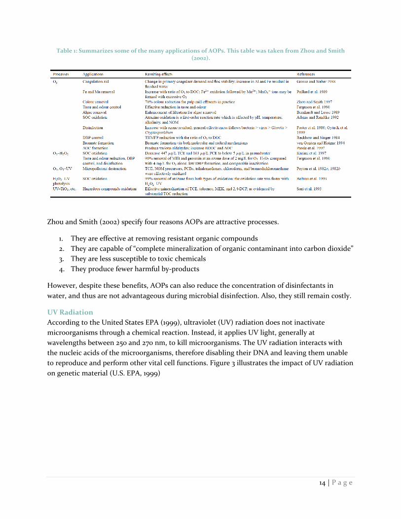
Table 1: Summarizes some of the many applications of AOPs. This table was taken from Zhou and Smith (2002).

Zhou and Smith (2002) specify four reasons AOPs are attractive processes.

1. They are effective at removing resistant organic compounds

2. They are capable of “complete mineralization of organic contaminant into carbon dioxide”

3. They are less susceptible to toxic chemicals

4. They produce fewer harmful by-products

However, despite these benefits, AOPs can also reduce the concentration of disinfectants in

water, and thus are not advantageous during microbial disinfection. Also, they still remain costly.

UV Radiation

According to the United States EPA (1999), ultraviolet (UV) radiation does not inactivate

microorganisms through a chemical reaction. Instead, it applies UV light, generally at

wavelengths between 250 and 270 nm, to kill microorganisms. The UV radiation interacts with

the nucleic acids of the microorganisms, therefore disabling their DNA and leaving them unable

to reproduce and perform other vital cell functions. Figure 3 illustrates the impact of UV radiation

on genetic material (U.S. EPA, 1999)

15 | P a g e

Figure 3: Impact of UV radiation on DNA. Demonstrates how UV radiation inactivates pathogens (DaRo UV)

According to the EPA (1999), UV radiation holds numerous advantages when compared to

conventional treatment methods. It is effective at eliminating most viruses, spores, and cysts; it

eliminates the need for chemical handling; there are no harmful residual effects post-treatment; it

is user-friendly; and it requires very little space and also very little contact time (20 to 30 seconds)

when compared to other disinfectants.

However, despite these advantages, the EPA (1999) also does recognize that there are

disadvantages. It does not inactivate all pathogens; organisms can sometimes repair the damage

UV radiation does to them; a maintenance program is necessary to control fouling in tubes;

turbidity can render it ineffective; and it is not quite as cost-effective as chlorination.

Membrane Filtration

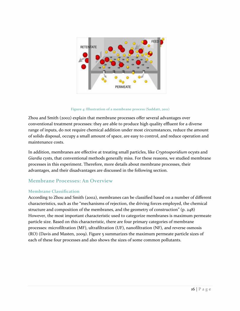
Membranes are semi-permeable barriers that separate materials based on their physical and/or

chemical properties. Figure 4 illustrates a membrane process. In this process, a solution is passed

over the membrane. Some of this solution, the permeate, travels through the membrane. Other

parts of this solution, the retentate, do not. The passage of materials through a membrane

generally requires a driving force, normally pressure (Davis and Masten, 2009).

16 | P a g e

Figure 4: Illustration of a membrane process (Saddatt, 2011)

Zhou and Smith (2002) explain that membrane processes offer several advantages over

conventional treatment processes: they are able to produce high quality effluent for a diverse

range of inputs, do not require chemical addition under most circumstances, reduce the amount

of solids disposal, occupy a small amount of space, are easy to control, and reduce operation and

maintenance costs.

In addition, membranes are effective at treating small particles, like Cryptosporidium ocysts and

Giardia cysts, that conventional methods generally miss. For these reasons, we studied membrane

processes in this experiment. Therefore, more details about membrane processes, their

advantages, and their disadvantages are discussed in the following section.

Membrane Processes: An Overview

Membrane Classification

According to Zhou and Smith (2002), membranes can be classified based on a number of different

characteristics, such as the “mechanisms of rejection, the driving forces employed, the chemical

structure and composition of the membranes, and the geometry of construction” (p. 248)

However, the most important characteristic used to categorize membranes is maximum permeate

particle size. Based on this characteristic, there are four primary categories of membrane

processes: microfiltration (MF), ultrafiltration (UF), nanofiltration (NF), and reverse osmosis

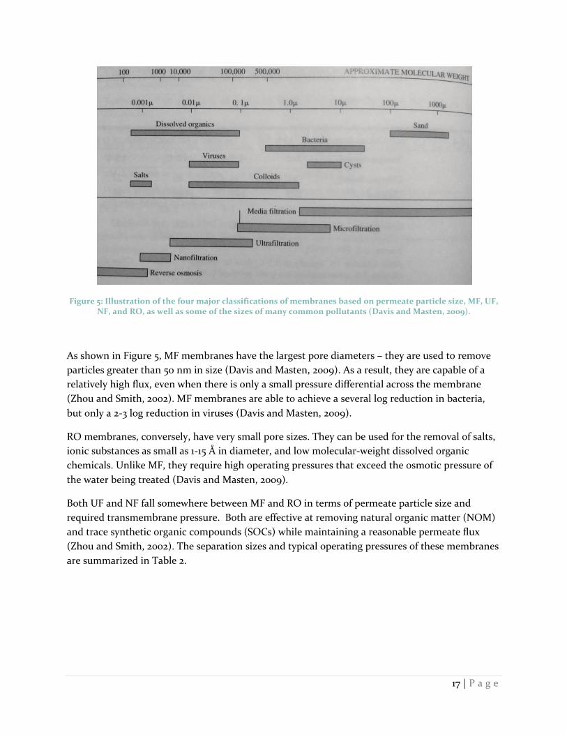
(RO) (Davis and Masten, 2009). Figure 5 summarizes the maximum permeate particle sizes of

each of these four processes and also shows the sizes of some common pollutants.

17 | P a g e

Figure 5: Illustration of the four major classifications of membranes based on permeate particle size, MF, UF, NF, and RO, as well as some of the sizes of many common pollutants (Davis and Masten, 2009).

As shown in Figure 5, MF membranes have the largest pore diameters – they are used to remove

particles greater than 50 nm in size (Davis and Masten, 2009). As a result, they are capable of a

relatively high flux, even when there is only a small pressure differential across the membrane

(Zhou and Smith, 2002). MF membranes are able to achieve a several log reduction in bacteria,

but only a 2-3 log reduction in viruses (Davis and Masten, 2009).

RO membranes, conversely, have very small pore sizes. They can be used for the removal of salts,

ionic substances as small as 1-15 Å in diameter, and low molecular-weight dissolved organic

chemicals. Unlike MF, they require high operating pressures that exceed the osmotic pressure of

the water being treated (Davis and Masten, 2009).

Both UF and NF fall somewhere between MF and RO in terms of permeate particle size and

required transmembrane pressure. Both are effective at removing natural organic matter (NOM)

and trace synthetic organic compounds (SOCs) while maintaining a reasonable permeate flux

(Zhou and Smith, 2002). The separation sizes and typical operating pressures of these membranes

are summarized in Table 2.

18 | P a g e

Table 2: Summary of membrane classifications based on permeate particle size.

Membrane Separation Size (µm)

Main Mechanisms

Typical Transmembrane pressure (MPa)

Permeate Flux

RO <0.001 Diffusion + Exclusion

5-8 Low

NF 0.001-0.008 Diffusion + Exclusion

0.5-1.5 Medium

UF 0.003-0.1 Sieving 0.05-0.5 High

MF >0.05 Sieving 0.03-0.3 High

Membrane Fouling

Though diverse in structure and performance, there are still drawbacks that apply to nearly all

membrane processes. The biggest of these drawbacks is membrane fouling, which is primarily

responsible for preventing the widespread adoption of membrane technologies (Davis and

Masten, 2009). Membrane fouling is caused by the deposition of pollutants on the membrane

surface or from adsorption of pollutants into membrane pores (Huang et al., 2012). It leads to

reduced flux and therefore increased energy usage over time. It also often creates the need for

chemical cleaning, which further increases cost and maintenance requirements (Huang et al.,

2012). This section provides further background on membrane fouling.

Description of Membrane Fouling

Marshall, Munro and Tragardh (1993) write that flux loss due to fouling occurs in three phases.

These three phases are shown in Figure 6. In the first phase, which lasts approximately one

minute, flux loss is primarily caused by concentration polarization. Figure 7 illustrates

concentration polarization. Concentration polarization occurs because the solute that is rejected

by the membrane builds up at the membrane surface. The concentration of this solute, then, is

higher at the membrane surface (Cm) than it is in the bulk solution (Cb). If Cm grows large enough,

a gel layer with solute concentration Cg forms. This gel layer adds additional resistance (Rg) that,

ultimately, reduces the flux (McCabe, Smith and Harriott, 1956).

19 | P a g e

Figure 6: The three phases of fouling. In the first phase, which lasts roughly one minute, flux loss is primarily caused by concentration polarization. In the second phase, which lasts between one and three hours, the flux declines at a moderate rate due to protein deposition on the membrane surface. And in the final phase, which

continues indefinitely, the flux declines slowly due to further protein deposition.

Figure 7: Illustration of concentration polarization, which leads to the first phase of flux loss during membrane filtration.

Concentration polarization is dictated by the hydrodynamic conditions of the membrane system

(Marshall et al., 1993). It can be controlled by a “cross-flow membrane module by means of

20 | P a g e

construction,” velocity adjustment, pulsation, ultrasound, or electric field generation

(Koltuniewicz and Noworyta) and is always reversible.

In the second phase of flux decline, the flux decreases moderately and is a result of protein

deposition on the membrane surface. It is likely that proteins initially adsorb onto the membrane

surface as a monolayer until a complete surface layer forms, resulting in reduced membrane flux.

The third phase of flux decline occurs when there is further protein deposition onto this

monolayer.

Although Goosen et al. (2005) explain that a number of different substances can cause fouling,

including bacteria, humic acids, and inorganics, this study focuses on fouling caused by proteins

because proteins were the only pollutants that this study tested experimentally. It is generally

accepted that protein adsorption, however, plays an important role in membrane fouling

(Marshall et al., 1993).

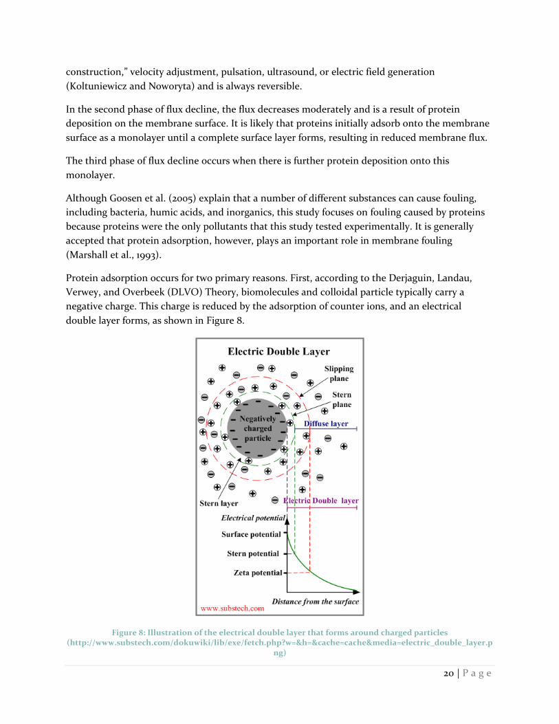
Protein adsorption occurs for two primary reasons. First, according to the Derjaguin, Landau,

Verwey, and Overbeek (DLVO) Theory, biomolecules and colloidal particle typically carry a

negative charge. This charge is reduced by the adsorption of counter ions, and an electrical

double layer forms, as shown in Figure 8.

Figure 8: Illustration of the electrical double layer that forms around charged particles (http://www.substech.com/dokuwiki/lib/exe/fetch.php?w=&h=&cache=cache&media=electric_double_layer.p

ng)

21 | P a g e

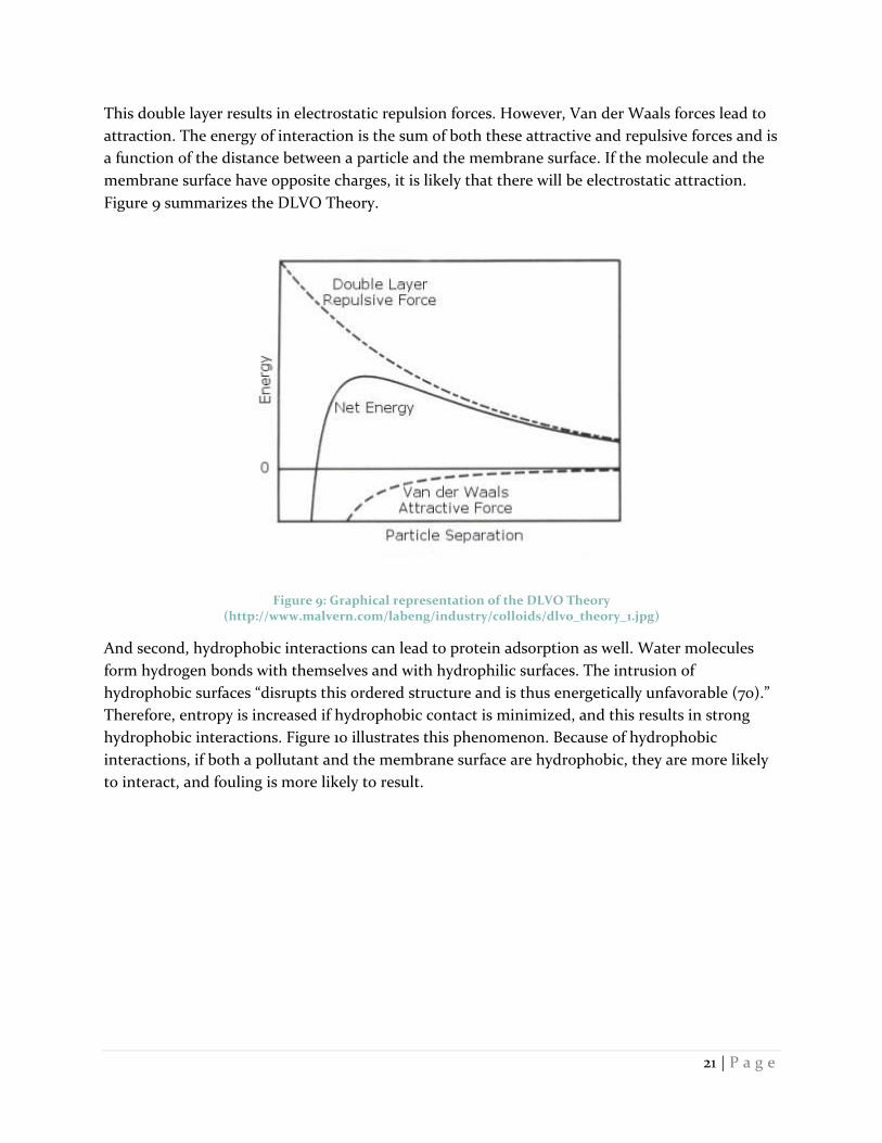
This double layer results in electrostatic repulsion forces. However, Van der Waals forces lead to

attraction. The energy of interaction is the sum of both these attractive and repulsive forces and is

a function of the distance between a particle and the membrane surface. If the molecule and the

membrane surface have opposite charges, it is likely that there will be electrostatic attraction.

Figure 9 summarizes the DLVO Theory.

Figure 9: Graphical representation of the DLVO Theory (http://www.malvern.com/labeng/industry/colloids/dlvo_theory_1.jpg)

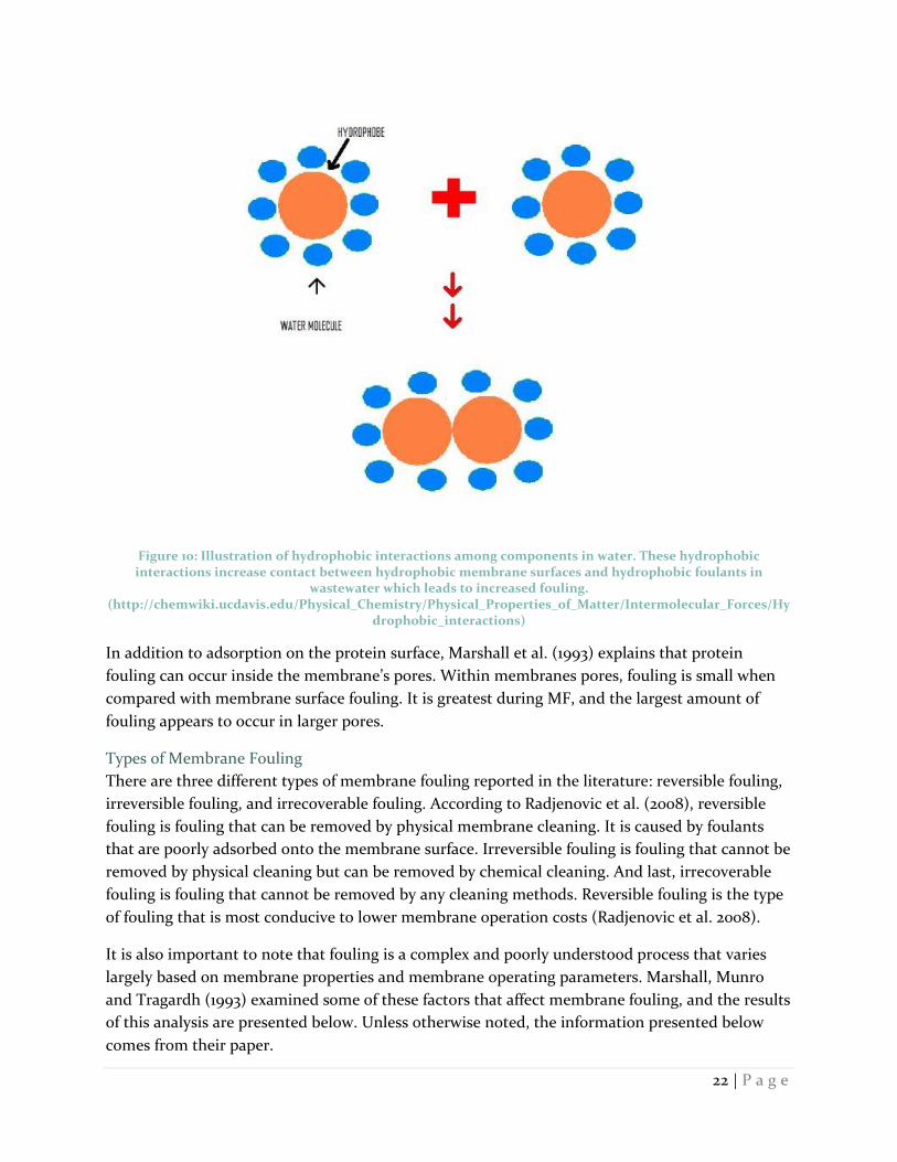
And second, hydrophobic interactions can lead to protein adsorption as well. Water molecules

form hydrogen bonds with themselves and with hydrophilic surfaces. The intrusion of

hydrophobic surfaces “disrupts this ordered structure and is thus energetically unfavorable (70).”

Therefore, entropy is increased if hydrophobic contact is minimized, and this results in strong

hydrophobic interactions. Figure 10 illustrates this phenomenon. Because of hydrophobic

interactions, if both a pollutant and the membrane surface are hydrophobic, they are more likely

to interact, and fouling is more likely to result.

22 | P a g e

Figure 10: Illustration of hydrophobic interactions among components in water. These hydrophobic interactions increase contact between hydrophobic membrane surfaces and hydrophobic foulants in

wastewater which leads to increased fouling. (http://chemwiki.ucdavis.edu/Physical_Chemistry/Physical_Properties_of_Matter/Intermolecular_Forces/Hy

drophobic_interactions)

In addition to adsorption on the protein surface, Marshall et al. (1993) explains that protein

fouling can occur inside the membrane’s pores. Within membranes pores, fouling is small when

compared with membrane surface fouling. It is greatest during MF, and the largest amount of

fouling appears to occur in larger pores.

Types of Membrane Fouling

There are three different types of membrane fouling reported in the literature: reversible fouling,

irreversible fouling, and irrecoverable fouling. According to Radjenovic et al. (2008), reversible

fouling is fouling that can be removed by physical membrane cleaning. It is caused by foulants

that are poorly adsorbed onto the membrane surface. Irreversible fouling is fouling that cannot be

removed by physical cleaning but can be removed by chemical cleaning. And last, irrecoverable

fouling is fouling that cannot be removed by any cleaning methods. Reversible fouling is the type

of fouling that is most conducive to lower membrane operation costs (Radjenovic et al. 2008).

It is also important to note that fouling is a complex and poorly understood process that varies

largely based on membrane properties and membrane operating parameters. Marshall, Munro

and Tragardh (1993) examined some of these factors that affect membrane fouling, and the results

of this analysis are presented below. Unless otherwise noted, the information presented below

comes from their paper.

23 | P a g e

Parameters that Impact Membrane Fouling

Feed Concentration

Increasing the feed concentration, in general, decreases the permeate flux. It also increases

reversible surface fouling, although it appears to have little impact on irreversible surface fouling.

However, it does increase the rate of membrane fouling when internal pore fouling dominates.

pH and Ionic Strength

The effect of pH and ionic strength on fouling is poorly understood, likely because it varies so

much depending on the protein and the membrane being studied. However, it does impact

fouling performance, though these impacts are variable depending on the system being analyzed.

Nevertheless, three general explanations have been provided for the effect of pH and ionic

strength on fouling. First, changes in protein “conformation and stability affect the tendency of

the protein to deposit on the membrane” (p. 83) Second, changes in the charge difference

between the protein and the membrane surface affect fouling. And third, changes in the protein’s

effective size “alter the porosity of the dynamic membrane” (p. 83).

Pre-filtration and the removal of aggregates

Pre-filtration and clarification of the feed material have both been shown to increase protein flux

during membrane filtration. Both these processes remove larger protein aggregates from the bulk

solution, and therefore these larger molecules cannot block membrane pores. This results in

reduced fouling.

Component Interactions

Component interactions in the bulk solution can impact membrane performance in a couple

ways. First, the presence of a larger component can increase the retention rate of smaller

components. This may be because, if the larger molecules are sufficiently retained by the

membrane, they could form a secondary membrane which reduces the passage of smaller

molecules through the primary membrane. Also, larger molecules pass more slowly, due to

friction, through membrane pores, which could further reduce the rate of passage of smaller

molecules. And last, in certain cases, specific component interactions within the feed can affect

retention rates.

Hydrophobicity

Reihanian, Robertson and Michaels (1983) found that filtration of a BSA solution through three

hydrophobic membranes (XM200, XM50, and PM30) led to reduced flux over time. This is likely

due to BSA adsorption on the membrane surface. However, when BSA solution was filtered

through highly hydrophilic cellulosic YM30 and poly-ion complex UM10 membranes, there was

no flux decline, indicating that were also was no BSA adsorption. This suggests that hydrophilic

membranes foul less easily than hydrophobic ones, a finding that has been widely reproduced.

Sheldon et al. suggest that one of the reasons for increased fouling on hydrophobic membranes is

that hydrophobic membrane surfaces help to denature proteins. They found that “the tertiary

protein structure of the globular protein [BSA] had, in some way, been disrupted and distorted by

24 | P a g e

interaction between BSA and polysulphone.” Normally, the outer layer of BSA is hydrophilic, but,

in this experiment, the BSA molecules adsorbed on the membrane surface had their hydrophobic

sites exposed.

Charge

The charge of the membrane surface is dependent on a number of factors including the PH and

ionic strength of the feed solution and the membrane material. Generally speaking, higher

permeate fluxes are observed if the charge of the membrane is similar to that of the protein being

filtered.

Surface roughness

An increase in surface roughness increases the likelihood of protein adsorption. However, it also

affects “the nature of the dynamic membrane” (p. 88). A rough membrane surface can reduce the

“completeness” of the dynamic membrane, which can in turn impact fouling.

Porosity and pore size distribution

Porosity and pore size distribution are important parameters in membrane performance. They

have a large impact on membrane selectivity; membranes with a wide pore size distribution will

be less selective than membranes with a low pore size distribution, assuming the average pore

sizes are the same.

Also, porosity and pore size distribution impact fouling. In general, membrane fouling is most

prevalent in membranes with low porosity and high heterogeneity. Greater heterogeneity leads to

a greater velocity normal to the membrane surface, which increases the rate of protein deposition,

which in turn leads to greater fouling.

Fouling can also impact the pore size distribution on a membrane surface. Studies have shown

that when fouling occurs, porosity and pore size distribution both decrease. Small pores become

blocked, and large pores decrease in size. This leads to a reduction in the number of small and

large pores and an increase in the number of medium sized pores.

Pore size

Pore size affects membrane performance in several ways. Many researchers have observed that

increased pore size, and thus decreased intrinsic membrane resistance, leads to increased

membrane fouling and, in some cases, lower permeate flux. Because of this, there is an optimal

pore size for particular membrane systems. Below this optimal pore size, membrane resistance

dominates and restricts permeate flow. Above this optimal pore size, fouling dominates and

restricts permeate flow. This optimal pore size is dependent on velocity.

Also, pore size is not necessarily the most important factor; rather, but the protein to pore size

ratio may be more important.

25 | P a g e

Transmembrane pressure

Increasing transmembrane pressure (TMP) increases permeate flux but also increases protein

fouling. However, there is an optimal TMP, and after this point, further increasing the TMP will

not lead to an increase in permeate flux. This optimal TMP decreases as pore size increases.

Higher TMP, studies found, also led to lower flux recovery after flushing, which suggests that

more fouling occurred when compared to lower TMP.

Cross-flow velocity and turbulence promoters

Generally, increasing cross-flow velocity results in an increase in permeate flux. Membrane

resistance decreases, which suggests that fouling and concentration polarization decrease as well.

Increased flux recovery is associated with higher cross flow velocity as well, which, again, suggests

less membrane fouling occurs.

Backflushing

The results of backflusing in UF and MF are varied. Some studies show that it is effective, while

others observe little difference. If accumulation of particles takes place on the membrane surface,

backflushing will likely be effective. However, if accumulation of particles takes place in

membrane pores or if particles are tightly adsorbed onto the membrane surface, backflushing will

likely not be very effective.

Temperature

Generally, increasing the temperature lowers the viscosity of the permeate and increases

permeate flux. In addition, it increases diffusivity, which helps to disperse the polarized layer in

membrane filtration.

Strategies to Address Membrane Fouling

Taking to consideration all of these factors that impact membrane fouling performance, several

strategies have been developed to help reduce membrane fouling, including microfiltration,

coagulation and flocculation, and membrane surface-modification. This study focuses on

membrane surface modification.

Membrane Surface Modification

Currently, organic polymers are the most commonly used materials for commercial membranes.

However, organic polymers have a hydrophobic surface which, as observed in many studies,

makes them particularly susceptible to membrane fouling (Su et al., 2011; Yu et al., 2005; Choi et

al., 2002). Fouling is more severe in hydrophobic membranes because of hydrophobic interactions

between solutes, microbial cells, and membrane material (Choi et al., 2002).

As a result, there has been significant interest recently in discovering ways to improve the

hydrophilicity of organic polymer membranes (Shen et al., 2011). Wu et al. (2008) explain that

several methods have been employed to modify membrane surfaces to make them more

hydrophilic, including the application of ultraviolet radiation, blending with hydrophilic

materials, graft polymerization, and plasma grafting. Of these methods, blending with hydrophilic

26 | P a g e

materials, particularly inorganic nanoparticles, has attracted the most attention because it

requires mild synthesis conditions during membrane preparation (Genne, Kuypers and Leysen,

1996).

Li et al. (2008) write that there are three methods commonly used to blend inorganic materials

with polymer membranes: (1) disperse nanoparticles in the casting solution directly and prepare

the composite membranes via phase inversion; (2) add prepared sol containing nanoparticles in

the casting solution and prepare the composite membranes via phase inversion; and (3), dip the

prepared membrane in an aqueous suspension containing nanoparticles and prepare the

composite membranes via self-assembly (Li et al., 2009). Several studies have applied these

methods to blend different nanoparticles with organic polymer membranes. The nanoparticles

used include TiO2 (Li et al., 2009; Wu et al., 2008) SiO2 (Huang et al., 2012; Shen et al., 2011), ZrO2

(Maximous et al., 2010; Bottino, Capannelli and Comite, 2002; Genne, Kuyperes and Leysen, 1996),

and ZnO (Shen et al., 2012). Many of these studies are summarized in Table 3.

Table 3: Summary of sources that have studied the impact of inorganic nanoparticles on membrane antifouling performance

TiO2 ZrO2 SiO2 ZnO

Source

Jing-Feng

Li et al.

2008

Jian-Hua Li

et al. 2008

Wu et al.

2008

Maximous

et al. 2009

Shen et al.

2011

Huang et

al. 2012

Shen et al.

2012

Anti-fouling

ability Enhanced Enhanced

Enhanced

to optimal

value

Enhanced

to optimal

value

Enhanced

to optimal

value

Enhanced

to optimal

value

Enhanced

to optimal

value

Hydrophilicity Enhanced Enhanced Enhanced Enhanced Enhanced

Enhanced

to optimal

value

Polymer

material PES SMA/PVDF PES PES PES

PES

Of these nanoparticles, TiO2 has been studied the most thoroughly due to its stability, availability,

(Wu et al., 2008) high hydrophilicity, and photocatalytic potential (Li et al., 2009). Jing-Feng Li et

al. (2008) dispersed varying concentrations of TiO2 nanoparticles (0-5 wt %) in polyethersulfone

(PES) casting solutions and prepared composite membranes via phase inversion. They found that

the composite membranes had enhanced thermal stability, hydrophilicity, and permeation

performance. They recommended an optimal loading rate of 1-2 wt % TiO2. Wu et al. (2008) also

prepared TiO2/PES composite membranes via nanoparticle dispersion and phase inversion. They

27 | P a g e

confirmed Jing-Feng Li et al.’s findings that the addition of TiO2 enhanced the hydrophilicity,

thermal stability, and mechanical strength of the membrane. However, they recommended an

optimal TiO2 loading rate of 0.5 wt % rather than 1-2 wt %. Jian-Hua Li et al. (2008) modified poly

(styrene-alt-maleic anhydride)/poly(vinylidene fluoride) (SMA/PVDF) to contain TiO2

nanoparticles via the self-assembly method. They also confirmed that the modified membranes

had enhanced hydrophilicity and superior permeability.

SiO2, though not as widely studied as TiO2, has also been analyzed. Shen et al. (2011) prepared

PES/SiO2 composite membranes (0-5 wt % SiO2) by the phase inversion method. They found that

pure and raw water flux increased, hydrophilicity was enhanced, and anti-fouling ability increased

with the addition of SiO2. Huang et al. (2012) prepared mesoporous silica (MS) modified PES

membranes via phase inversion. They found that the MS improved membrane hydrophilicity,

porosity, anti-fouling ability, and thermal stability. They recommend an optimal MS loading rate

of 2 wt %.

A third nanoparticle that has been studied for membrane modification is ZrO2. Maximous et al.

(2010) prepared PES/ZrO2 composite membranes (0, 0.01, 0.03, 0.05, 0.07, and 0.1 PES/ZrO2

weight ratios) via phase inversion and used these membranes for activated sludge filtration to

study their fouling characteristics. They found that the addition of ZrO2 particles improved

mechanical strength and anti-fouling ability. They recommend an optimal ZrO2 loading rate of

0.05 ZrO2/PES. Two older studies (Bottino, Capannelli, and Comite, 2002; Genne, Kuypers and

Leysen, 1996) also prepared ZrO2 composite membranes. Though their analyses were not as

thorough as those conducted by Maximous et al., both confirmed that permeability increased

with the addition of ZrO2.

Though less studied than the three other aforementioned particles, ZnO’s effect on membrane

performance has also been analyzed. Shen et al. (2012) prepared PES/ZnO composite membrane

via phase inversion. They found that the addition of ZnO improves hydrophilicity, thermal

decomposition temperature, water flux, and porosity.

All these experiments suggest that modifying membrane surfaces with TiO2, SiO2, ZrO2 and ZnO

both improves membrane hydrophilicity and enhances membrane antifouling performance.

However, no study has compared which of these inorganic nanoparticles is most effective.

Therefore, in this study, these inorganic nanoparticles were compared. To do this, five types of

membrane were prepared. One of these membranes was not modified with inorganic

nanoparticles, and the other four were each modified with either TiO2, SiO2, ZrO2 and ZnO. The

following section explains the processes used to prepare these membranes.

Membrane Preparation

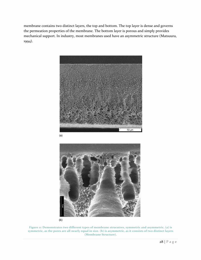
Synthetic membranes have two primary types of structures: symmetric and asymmetric. Figure 11

demonstrates the difference between these structures. In symmetric membranes, the diameter of

the pores is nearly constant throughout the entire cross section. Conversely, in asymmetric

membranes, the pore size is not constant throughout the entire cross section. Instead, the

28 | P a g e

membrane contains two distinct layers, the top and bottom. The top layer is dense and governs

the permeation properties of the membrane. The bottom layer is porous and simply provides

mechanical support. In industry, most membranes used have an asymmetric structure (Matsuura,

1994).

Figure 11: Demonstrates two different types of membrane strucutres, symmetric and asymmetric. (a) is symmetric, as the pores are all nearly equal in size. (b) is asymmetric, as it consists of two distinct layers

(Membrane Structure).

29 | P a g e

Many methods have been developed to prepare asymmetric membranes (Matsura, 1994). Of these

methods, phase inversion techniques are most commonly used.

Phase Inversion

Kools and Catherina (1998) explain that there are three ways to induce phase inversion:

temperature induced phase inversion, reaction induced phase inversion, and dry-wet phase

inversion. Of these, dry-wet phase inversion, or the Loeb-Sourirajan technique, is most common,

and this was the technique used in this experiment.

For the Loeb-Sourirajan technique, a polymer solution is prepared by mixing a polymer and a

solvent. This solution is than cast on a glass plate, and this plate is immersed into a gelation bath.

The process involves two desolvation steps. First, when the solution is cast onto the glass plate,

the solvent evaporates. This facilitates the formation of a thick skin layer at the top of the

membrane. And second, when the solution is immersed into the gelation bath, solvent-nonsolvent

exchange occurs. The nonsolvent diffuses into the polymer film while the solvent diffuses out.

Due to these steps, the polymer solidifies into a porous membrane (ibid). Figure 12 illustrates this

process:

Figure 12: Schematic representation of three dry-wet separation processes. A) precipitation with nonsolvent vapor; B) evaporation of solvent; C) immersion precipitation. The arrows denote the net direction of diffusion

for each step. Polymer, solvent, and nonsolvent are represented by P, S, and NS, respectively (Kools and Catherina, 1998).

For this experiment, the solvent used was dimethylacetmaide (DMAc), the nonsolvent was water,

and the polymer was polyethersulfone. Figure 13 shows the ternary phase diagram for the phase

inversion process in this experiment. The line with points A, B, C, and D denotes the path that the

30 | P a g e

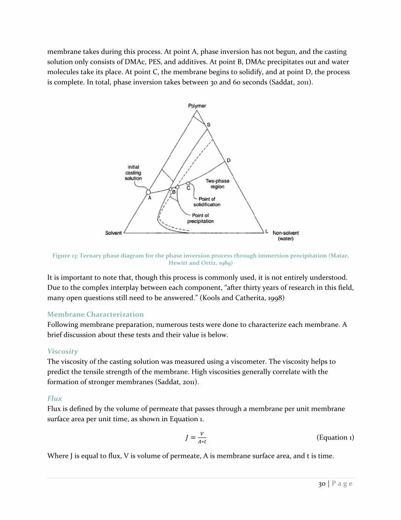
membrane takes during this process. At point A, phase inversion has not begun, and the casting

solution only consists of DMAc, PES, and additives. At point B, DMAc precipitates out and water

molecules take its place. At point C, the membrane begins to solidify, and at point D, the process

is complete. In total, phase inversion takes between 30 and 60 seconds (Saddat, 2011).

Figure 13: Ternary phase diagram for the phase inversion process through immersion precipitation (Matar, Hewitt and Ortiz, 1989)

It is important to note that, though this process is commonly used, it is not entirely understood.

Due to the complex interplay between each component, “after thirty years of research in this field,

many open questions still need to be answered.” (Kools and Catherita, 1998)

Membrane Characterization

Following membrane preparation, numerous tests were done to characterize each membrane. A

brief discussion about these tests and their value is below.

Viscosity

The viscosity of the casting solution was measured using a viscometer. The viscosity helps to

predict the tensile strength of the membrane. High viscosities generally correlate with the

formation of stronger membranes (Saddat, 2011).

Flux

Flux is defined by the volume of permeate that passes through a membrane per unit membrane

surface area per unit time, as shown in Equation 1.

(Equation 1)

Where J is equal to flux, V is volume of permeate, A is membrane surface area, and t is time.

31 | P a g e

Flux is an important indicator of membrane performance. Larger fluxes results in more rapid

filtration and therefore reduced operating and implementation costs.

Porosity

Porosity is a measure of void space within a membrane. Porosity is calculated using Equation 2.

(Equation 2)

The total volume of the membrane is determined through physical measurements. The volume of

the void space is determined by comparing the mass of a membrane when it is wet and when it is

dry. The difference between these masses is equal to the mass of water occupying the void space.

Using the density of water, the volume of void space, then, can also be determined.

Porosity is important because it impacts flux.

Rejection Rate

Rejection rate measures how effectively a membrane can filter a particular pollutant. It is

important because it dictates the quality of the permeate stream. Rejection rate is calculated

using Equation 3.

(

) (Equation 3)

Where Cp is the concentration of a particular component in the permeate stream, and Cf is the

concentration of that same component in the solution prior to filtration.

Scanning Electron Microscope

A Scanning electron microscope (SEM) scans samples with focused beams of electrons. These

electrons “interact with electrons in the sample” being studied, thereby producing information

about the structure of the sample.

Images produced with a SEM elucidate the structure of particular membranes as well as the

thickness of the surface layer of asymmetric membranes.

Fourier Transform Infrared Spectroscopy

Fourier transform infrared spectroscopy (FTIR) is used to obtain the infrared spectrum of for a

particular sample. It collects data over a wide spectral range, and this data can be used to identify

specific functional groups that are present in the sample being studied.

For this experiment, FTIR was used to determine whether or not specific inorganic nanoparticles

were present on the surfaces of the prepared membranes.

X-ray Photoelectron Spectroscopy

X-ray photoelectron spectroscopy (XPS) is used to determine the elemental composition of the

surface of a particular sample. XPS irradiates a material with X-rays and then measures the kinetic

energy and number of electrons that escape the surface of the sample being analyzed. This data

32 | P a g e

can be used to determine the elements that are present on the sample surface. (Queen Mary

University London)

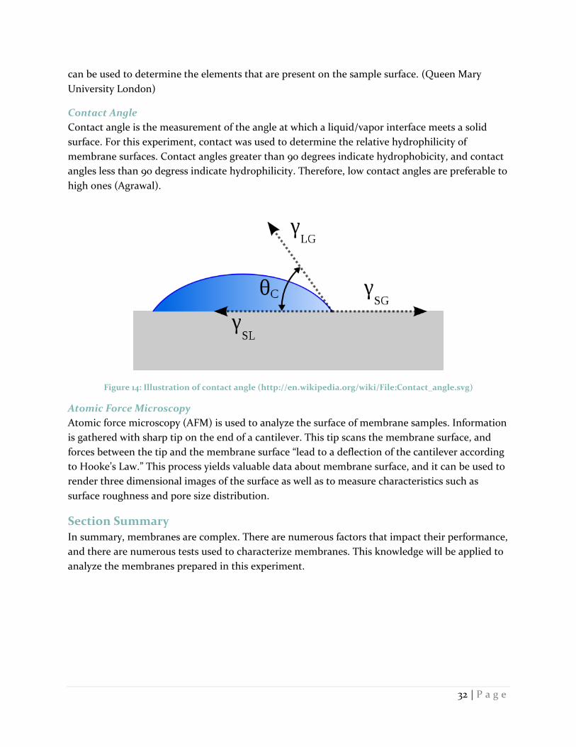
Contact Angle

Contact angle is the measurement of the angle at which a liquid/vapor interface meets a solid

surface. For this experiment, contact was used to determine the relative hydrophilicity of

membrane surfaces. Contact angles greater than 90 degrees indicate hydrophobicity, and contact

angles less than 90 degress indicate hydrophilicity. Therefore, low contact angles are preferable to

high ones (Agrawal).

Figure 14: Illustration of contact angle (http://en.wikipedia.org/wiki/File:Contact_angle.svg)

Atomic Force Microscopy

Atomic force microscopy (AFM) is used to analyze the surface of membrane samples. Information

is gathered with sharp tip on the end of a cantilever. This tip scans the membrane surface, and

forces between the tip and the membrane surface “lead to a deflection of the cantilever according

to Hooke’s Law.” This process yields valuable data about membrane surface, and it can be used to

render three dimensional images of the surface as well as to measure characteristics such as

surface roughness and pore size distribution.

Section Summary

In summary, membranes are complex. There are numerous factors that impact their performance,

and there are numerous tests used to characterize membranes. This knowledge will be applied to

analyze the membranes prepared in this experiment.

33 | P a g e

Methodology In this experiment, five distinct membranes were prepared: a pure PES membrane and four PES

membranes that were modified with different inorganic nanoparticles (TiO2, SiO2, ZnO, and

ZrO2). Following membrane preparation, several tests were conducted to characterize membrane

performance. This section discusses the methods used to both prepare and characterize the

membranes.

Membrane Preparation

All five membranes were prepared using the phase inversion method. For the phase inversion

method, the first step was to create a casting solution for each different membrane. However,

before the casting solutions were prepared, the inorganic nanoparticles needed to be prepared. If

added to the casting solution untreated, the inorganic nanoparticles would aggregate and the

modified membranes would not have been as effective, according to Shen et al. (2011). Therefore,

to increase their dispersability in the casting solution, the inorganic nanoparticles were treated

according to the method described by Shen et al. (2011), the details of which are described in the

section below.

Pre-treatment of inorganic nanoparticles

For each inorganic nanoparticles, 1000 mL of H2O were measured into two beakers. The pH of

each of these beakers was then lowered to 4.0, and a 3.5 weight percent sodium dodecyl sulfate

(SDS) solution was then created with this water. 5 g of inorganic nanoparticles were then added

to each 1000 mL solution, and the solution was then stirred for 8 hours. Following this stirring,

the solution was then vacuum filtered so as to isolate the inorganic nanoparticles. The isolated

nanoparticles were then vacuum dried for 8 hours at 60 degrees C to remove any remaining

water. After drying, the particles were ready for addition to the casting solutions.

Casting solution preparation

After treating the inorganic nanoparticles, the casting solutions were then ready to be prepared.

In total, five casting solutions were created, one for each membrane that was tested. Each casting

solution consisted of dimethylacetamide (DMAc) as the solvent, pure PES, and the additive

polyethylene glycol 400 (PEG 400). The casting solutions for the modified membranes also

contained inorganic nanoparticles. Figure 15 shows the weight percentages of each component

for the pure PES membrane casting solution, and Figure 16 shows the weight percentages of each

component for the modified membranes’ casting solutions. Tables 9-13 in Appendix 2 show the

mass of each component that was present in each casting solution.

34 | P a g e

Figure 15: Weight percentages of the components of the pure PES membrane

Figure 16: Weight percentages of the components of the four modified PES membranes

To prepare the pure PES casting solution, half of the necessary DMAc was first added to a 500 mL

flask. The PES was then added in small increments with regular mixing. After all the PES was

added, the remaining DMAc and the PEG 400 were then added as well. The solution was then

stirred in a water batch heater at 60 degrees C for 6-8 hours, or until all the PES had dissolved.

After stirring, the solution was then allowed to sit for at least 24 hours so as to eliminate all

bubbles.

PES 18%

DMAc 76%

PEG 400 6%

PES 18%

DMAc 75%

PEG 400 6% Nanoparticle

1%

35 | P a g e

To prepare the PES/inorganic nanoparticle casting solutions, half of the necessary DMAc was first

added to a 500 mL flask. The flask was then placed in a high speed stirring machine, and, little by

little, inorganic nanoparticles were added. After all the inorganic nanoparticles were added, the

solution was stirred for an additional ten minutes. After this stirring, the PES was then added

incrementally with regular mixing. After all the PES was added, the remaining DMAc and the

PEG 400 were then added as well. The solution was then stirred in a water batch heater at 60

degrees C for 6-8 hours, or until all the PES had dissolved.

Figure 17 is an image of three of the completed casting solutions.

Figure 17: Three of the completed casting solutions

Following the preparation of all five casting solutions, the viscosity of each casting solution was

then measured. After taking the viscosity measurements, membranes were then able to be

prepared.

Casting the Membranes

To create the membranes, the newly-prepared casting solutions were poured onto a glass plate,

and a machine evenly distributed the casting solutions across this plate. The machine was set to a

particular thickness so that the thickness of all the prepared membranes would be as equal as

36 | P a g e

possible. Figure 18 is an image of the glass plates that the casting solution is poured on, and Figure

19 is an image of the machine that evenly distributes the casting solutions across these plates.

Figure 18: The glass plates that the casting solutions are poured onto

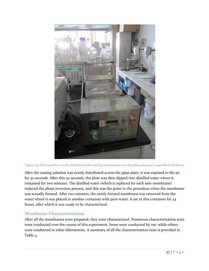
37 | P a g e

Figure 19: This machine evenly distributes the casting solutions across the glass plates at a specified thickness

After the casting solution was evenly distributed across the glass plate, it was exposed to the air

for 30 seconds. After this 30 seconds, the plate was then dipped into distilled water where it

remained for two minutes. The distilled water (which is replaced for each new membrane)

induced the phase inversion process, and this was the point in the procedure when the membrane

was actually formed. After two minutes, the newly-formed membrane was removed from the

water where it was placed in another container with pure water. It sat in this container for 24

hours, after which it was ready to be characterized.

Membrane Characterization

After all the membranes were prepared, they were characterized. Numerous characterization tests

were conducted over the course of this experiment. Some were conducted by me, while others

were conducted in other laboratories. A summary of all the characterization tests is provided in

Table 4.

38 | P a g e

Table 4: Summary of tests used to characterize prepared membranes

In this section, the methodology for the tests that I conducted will be described.

Pure water flux

After the membranes were prepared, the pure water flux at 0.03, 0.05, 0.07, 0.09, and 0.1 MPa was

measured for each. When the pressure was adjusted, at least 20 minutes passed before flux

measurements were taken. This allowed the membrane to reach a steady state flux. Once at least

20 minutes passed, the time it took to filter 40 g of water through each membrane was recorded.

From this data, the pure water flux was calculated at each different pressure.

Resistance

To calculate the intrinsic membrane resistance (Rm), the pure water flux data was graphed on a

curve (pure water flux versus pressure), and a linear curve was fit to this data. Rm was calculated

from this curve.

Rejection rate

To determine the rejection rate, a 1000 mg/L BSA solution was filtered through each membrane.

However, before this filtration occurred, the BSA solution needed to be prepared, and a

concentration curve needed to be created. The concentration curve allowed us to determine the

concentration of BSA in the permeate stream by calculating its absorbance.

BSA Concentration Curve

To create the BSA concentration curve, six solutions of BSA were created, all with different

concentrations of BSA (10, 100, 200, 400, 700, and 1000 mg/L BSA). The absorbance for each of

these pre-made solutions was calculated, and a graph was then created with absorbance data on

the y-axis and BSA concentration data on the x-axis. A linear curve was then fit to this data. With

this linear curve, the concentration of BSA could be determined with absorbance data.

After the BSA concentration curve was created, the 1000 mg/L BSA solution was filtered through

each membrane. The absorbance of the permeate stream was then calculated, and this

absorbance data was used to calculate the BSA concentration in the permeate stream. From this,

rejection rate for each of the membranes was determined.

Conducted by me Conducted by others

Pure Water Flux Fourier Transform Infrared Spectroscopy

Resistance X-ray Photoelectron Spectroscopy

Rejection Rate Atomic Force Microscopy

Flux Decline Scanning Electron Microscope

Flux Recovery Breaking Force

Zeta Potential Elongation Rate

Porosity Total Gravimetric Analysis

Contact Angle

39 | P a g e

Flux decline

To determine flux decline, again, a 1000 mg/L BSA solution was filtered through each membrane.

The permeate stream was diverted into a beaker, and the mass of this beaker was measured every

10 seconds. All this data was recorded by a computer and was later exported into Microsoft Excel.

Using Microsoft Excel, it was determined how the mass flow rate changed with time. From this, it

was determined how the flux changed with time, which in turn elucidated how much the flux was

reduced and how long it took for a steady state flux to be reached.

Flux recovery

After the flux decline experiments were finished, pure water was filtered through each of the

membranes, and a new pure water flux was determined.

Following the determination of this new pure water flux, each membrane underwent a series of

cleaning procedures. First, the membrane was cleaned with pure water. This was accomplished by

placing the membrane in a beaker of water and shaking the beaker for twenty minutes. After this

cleaning was finished, the pure water flux was measured again.

After the pure water cleaning, the membrane was cleaned with NaOH. This was accomplished by

letting the membrane sit in an NaOH solution for twenty minutes. After the NaOH cleaning, the

pure water flux was taken again.

After the NaOH cleaning, the membrane was then cleaned with NaOCl. Again, to accomplish this,

the membrane was placed in an NaOCl solution where it remained for twenty minutes. After this

twenty minutes was complete, the pure water flux was measured again.

After all the cleanings were complete, the new pure water fluxes measured after cleaning were

compared to the pure water fluxes before cleaning. From this data, the flux recovery ratio was

determined.

Porosity

To calculate the membrane porosity, the volume of a membrane sample was first determined.

Next, the weight of this membrane sample was calculated when wet. After this, the membrane

was dried for 8 hours at 60 degrees C, and the dry weight was then measured. From all this data,

the porosity of the membrane was determined. This was repeated for three sample for each

different membrane, and the values for each sample were averaged together.

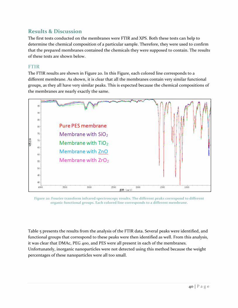
40 | P a g e

Results & Discussion The first tests conducted on the membranes were FTIR and XPS. Both these tests can help to

determine the chemical composition of a particular sample. Therefore, they were used to confirm

that the prepared membranes contained the chemicals they were supposed to contain. The results

of these tests are shown below.

FTIR

The FTIR results are shown in Figure 20. In this Figure, each colored line corresponds to a

different membrane. As shown, it is clear that all the membranes contain very similar functional

groups, as they all have very similar peaks. This is expected because the chemical compositions of

the membranes are nearly exactly the same.

Figure 20: Fourier transform infrared spectroscopy results. The different peaks correspond to different organic functional groups. Each colored line corresponds to a different membrane.

Table 5 presents the results from the analysis of the FTIR data. Several peaks were identified, and

functional groups that correspond to these peaks were then identified as well. From this analysis,

it was clear that DMAc, PEG 400, and PES were all present in each of the membranes.

Unfortunately, inorganic nanoparticles were not detected using this method because the weight

percentages of these nanoparticles were all too small.

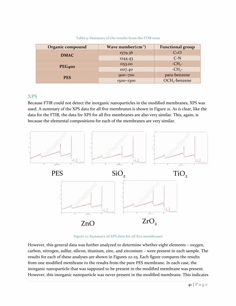
41 | P a g e

Table 5: Summary of the results from the FTIR tests

Organic compound Wave number(cm-1) Functional group

DMAC 1579.36 C=O

1244.43 C-N

PEG400 1153.00 -CH2-

1107.40 -CH2-

PES 900~700 para-benzene

1500~1300 OCH3-benzene

XPS

Because FTIR could not detect the inorganic nanoparticles in the modified membranes, XPS was

used. A summary of the XPS data for all five membranes is shown in Figure 21. As is clear, like the

data for the FTIR, the data for XPS for all five membranes are also very similar. This, again, is

because the elemental compositions for each of the membranes are very similar.

Figure 21: Summary of XPS data for all five membranes

However, this general data was further analyzed to determine whether eight elements – oxygen,

carbon, nitrogen, sulfur, silicon, titanium, zinc, and zirconium – were present in each sample. The

results for each of these analyses are shown in Figures 22-25. Each figure compares the results

from one modified membrane to the results from the pure PES membrane. In each case, the

inorganic nanoparticle that was supposed to be present in the modified membrane was present.

However, this inorganic nanoparticle was never present in the modified membrane. This indicates

PES SiO2 TiO2

ZnO ZrO2

42 | P a g e

that the methodology used succeeded in embedding inorganic nanoparticles on the membrane

surface.

Figure 22: Comparison of the XPS results for the SiO2 modified membrane and the pure PES membrane. The red lines correspond to the data for the SiO2 membrane, and the blue lines correspond to the data for the

pure PES membranes. As is clear, each membrane contained oxygen, carbon, nitrogen, and sulfur. However, only the SiO2 modified membrane contained silicon, as expected.

Figure 23: Comparison of the XPS results for the TiO2 modified membrane and the pure PES membrane. The red lines correspond to the data for the TiO2 membrane, and the gold lines correspond to the data for the

pure PES membranes. As is clear, each membrane contained oxygen, carbon, nitrogen, and sulfur. However, only the TiO2 modified membrane contained titanium, as expected.

Oxygen Carbon Nitrogen Sulfur

Si

Oxygen Carbon Nitrogen Sulfur

Ti

43 | P a g e

Figure 24: Comparison of the XPS results for the ZnO modified membrane and the pure PES membrane. The red lines correspond to the data for the ZnO membrane, and the blue lines correspond to the data for the

pure PES membranes. As is clear, each membrane contained oxygen, carbon, nitrogen, and sulfur. However, only the ZnO modified membrane contained zinc, as expected.

ZrO2

Figure 25: Comparison of the XPS results for the ZnO modified membrane and the pure PES membrane. The red lines correspond to the data for the ZnO membrane, and the purple lines correspond to the data for the pure PES membranes. As is clear, each membrane contained oxygen, carbon, nitrogen, and sulfur. However,

only the ZrO2 modified membrane contained zirconium, as expected.

Oxygen Carbon Nitrogen Sulfur

Zn

Oxygen Carbon Nitrogen Sulfur

Zr

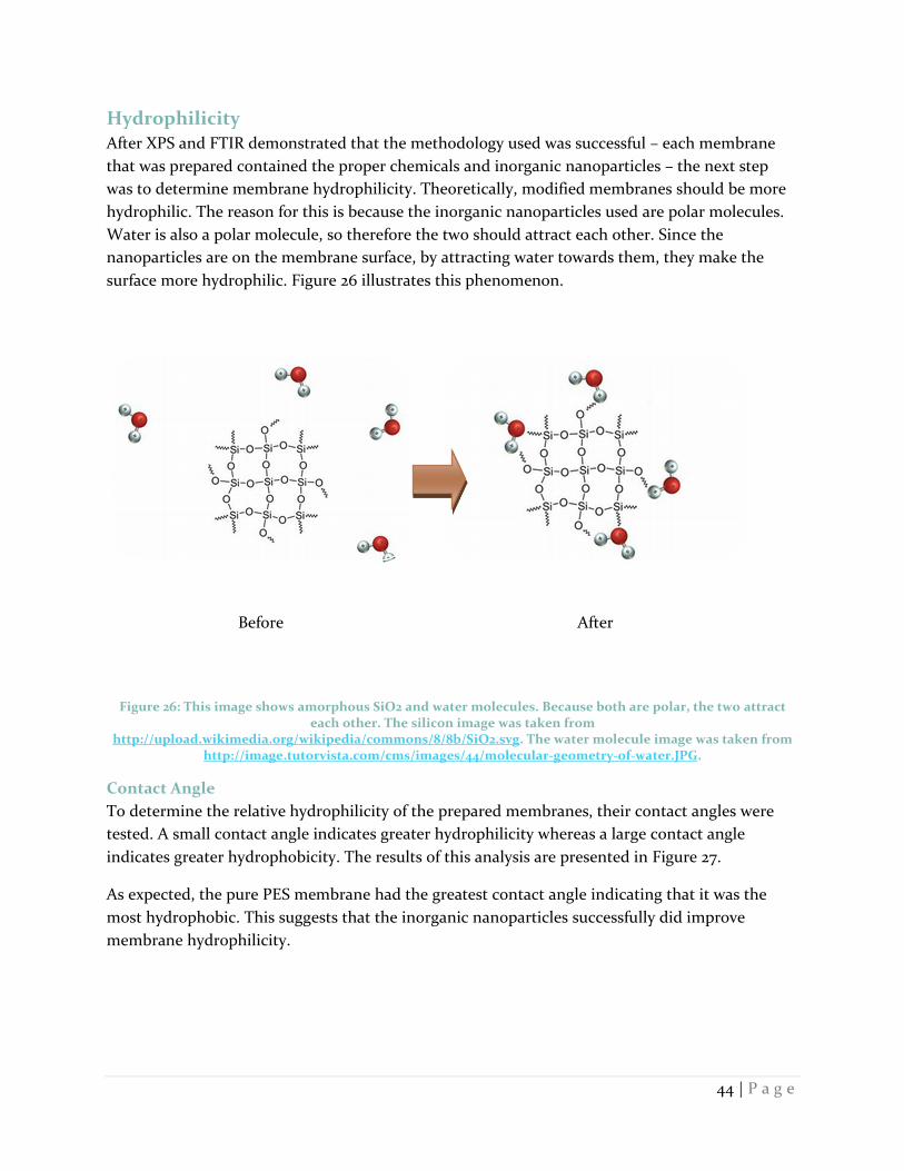
44 | P a g e

Hydrophilicity

After XPS and FTIR demonstrated that the methodology used was successful – each membrane

that was prepared contained the proper chemicals and inorganic nanoparticles – the next step

was to determine membrane hydrophilicity. Theoretically, modified membranes should be more

hydrophilic. The reason for this is because the inorganic nanoparticles used are polar molecules.

Water is also a polar molecule, so therefore the two should attract each other. Since the

nanoparticles are on the membrane surface, by attracting water towards them, they make the

surface more hydrophilic. Figure 26 illustrates this phenomenon.

Figure 26: This image shows amorphous SiO2 and water molecules. Because both are polar, the two attract each other. The silicon image was taken from

http://upload.wikimedia.org/wikipedia/commons/8/8b/SiO2.svg. The water molecule image was taken from http://image.tutorvista.com/cms/images/44/molecular-geometry-of-water.JPG.

Contact Angle

To determine the relative hydrophilicity of the prepared membranes, their contact angles were

tested. A small contact angle indicates greater hydrophilicity whereas a large contact angle

indicates greater hydrophobicity. The results of this analysis are presented in Figure 27.

As expected, the pure PES membrane had the greatest contact angle indicating that it was the

most hydrophobic. This suggests that the inorganic nanoparticles successfully did improve

membrane hydrophilicity.

Before After

45 | P a g e

Figure 27: Contact angles of each of the prepared membranes. PES had the largest contact angle followed by ZrO2, SiO2, TiO2, and ZnO.

Figure 28 compares each of the modified membranes. It illustrates the reduction of each

membrane’s contact angle relative to the contact angle of the pure PES membrane. ZnO showed

the greatest reduction in contact angle (13.5%), followed by TiO2 (8.3%), SiO2 (7.9%), and ZrO2

(7.6%). These results indicate that ZnO was the most hydrophilic of the five prepared

membranes.

20.00

30.00

40.00

50.00

60.00

70.00

80.00

PES PES+SiO2 PES+TiO2 PES+ZnO PES+ZrO2

46 | P a g e

Figure 28: Reduction in the contact angle of the four modified membranes as compared to the pure PES membrane. The ZnO membrane showed the greatest contact angle reduction, followed by TiO2, SiO2, and

then ZrO2.

Antifouling Performance

After determining that the contact angles for each of the modified membranes had been reduced

by the inorganic nanoparticles, the next step was to determine if this reduction in contact angle

led to enhanced antifouling performance. To accomplish this, flux reduction curves were

generated from the BSA filtration data (see “Flux Decline” section in methodology for more

details). These curves are presented in Figure 29. All these curves correspond well with theory.

Each shows three distinct phases of fouling, as described by Marshall, Munro and Tragardh (1993).

The first, which is rapid, occurs in the first minute and is the result of concentration polarization.

The second, which reduces flux at a moderate rate and lasts significantly longer than the first

phase (up to seven hours in the case of this experiment), is caused by protein deposition on the

membrane surface. And the third phase is where the curves flatten and the flux remains nearly

constant (Marshall, Munro and Tragardh, 1993).

0

2

4

6

8

10

12

14

16

PES+SiO2 PES+TiO2 PES+ZnO PES+ZrO2

% R

ed

uct

ion

47 | P a g e

Figure 29: Flux decline curves for all five prepared membranes. On the x-axis is flux (L/m2*hr), and on the x-

axis is the time when the flux measurement was taken (minutes). The longer it takes for the graph to plateau, the better the antifouling performance.

The time it takes for the third phase to be reached is indicative of anti-fouling performance. The

longer it takes to reach the third phase, the more time it took for proteins to form a monolayer on

the membrane surface. Therefore, the membrane that takes the longest to reach the third phase is

the least likely to foul.

Figure 30 illustrates the time it took each membrane to reach the third phase. Of all the

membranes, PES took the least amount of time, by far (~20 minutes), to reach this phase. This

indicates that the pure PES membrane fouled the most easily, which, in turn, indicates that the

addition of the inorganic nanoparticles did enhance membrane anti-fouling performance, as

expected.

ZnO, surprisingly, took the second least amount of time to reach the third phase of flux reduction

(~200 minutes), which indicates that it fouled the second most easily. This was unexpected

because it showed the greatest reduction in hydrophilicity, which should enhance antifouling

performance. This suggests that factors other than membrane hydrophilicity, like porosity,

roughness, and pore distribution, also affect membrane anti-fouling performance, and some of

these factors will be discussed later in the paper to explain why the ZnO-modified membrane’s

antifouling performance was improved the least. SiO2 and TiO2 both took the longest to reach

phase three (~400 minutes), which indicates that they had they had the best anti-fouling

performance.

PES SiO2 TiO2

ZnO ZrO2

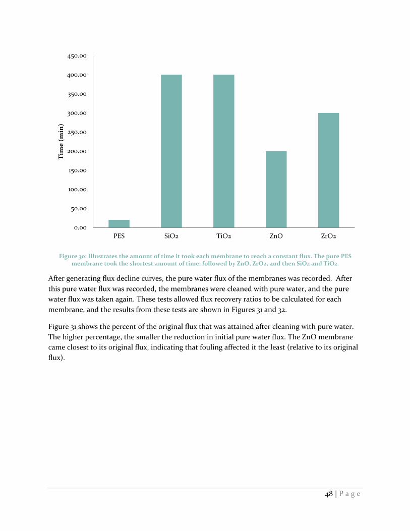
48 | P a g e

Figure 30: Illustrates the amount of time it took each membrane to reach a constant flux. The pure PES membrane took the shortest amount of time, followed by ZnO, ZrO2, and then SiO2 and TiO2.

After generating flux decline curves, the pure water flux of the membranes was recorded. After

this pure water flux was recorded, the membranes were cleaned with pure water, and the pure

water flux was taken again. These tests allowed flux recovery ratios to be calculated for each

membrane, and the results from these tests are shown in Figures 31 and 32.

Figure 31 shows the percent of the original flux that was attained after cleaning with pure water.

The higher percentage, the smaller the reduction in initial pure water flux. The ZnO membrane

came closest to its original flux, indicating that fouling affected it the least (relative to its original

flux).

0.00

50.00

100.00

150.00

200.00

250.00

300.00

350.00

400.00

450.00

PES SiO2 TiO2 ZnO ZrO2

Tim

e (

min

)

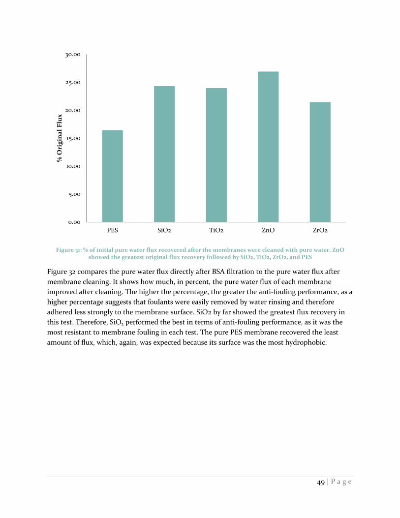
49 | P a g e

Figure 31: % of initial pure water flux recovered after the membranes were cleaned with pure water. ZnO showed the greatest original flux recovery followed by SiO2, TiO2, ZrO2, and PES

Figure 32 compares the pure water flux directly after BSA filtration to the pure water flux after

membrane cleaning. It shows how much, in percent, the pure water flux of each membrane

improved after cleaning. The higher the percentage, the greater the anti-fouling performance, as a

higher percentage suggests that foulants were easily removed by water rinsing and therefore

adhered less strongly to the membrane surface. SiO2 by far showed the greatest flux recovery in

this test. Therefore, SiO2 performed the best in terms of anti-fouling performance, as it was the

most resistant to membrane fouling in each test. The pure PES membrane recovered the least

amount of flux, which, again, was expected because its surface was the most hydrophobic.

0.00

5.00

10.00

15.00

20.00

25.00

30.00

PES SiO2 TiO2 ZnO ZrO2

% O

rig

ina

l F

lux

50 | P a g e

Figure 32: Percent improvement in flux after cleaning with pure water of all five prepared membranes

Summary of Membrane Antifouling Performance

The introduction of inorganic nanoparticles reduced the hydrophilicity of PES membranes. The

ZnO’s hydrophilicty was reduced the most followed by TiO2’s, SiO2’s, and ZrO2’s. TiO2 and SiO2

took the longest to reach the third stage of flux decline, indicating that they were most resistant

to membrane fouling, and both also showed the greatest improvement in flux when they were

cleaned with pure water after BSA filtration. However, ZnO came closest to its original pure water

flux after being cleaned with pure water, and SiO2 demonstrated the greatest improvement in flux

after being cleaned. The pure PES membrane performed the worst in all these experiments.

Based on these tests, SiO2 demonstrated the best antifouling performance. It took the longest to

foul and it demonstrated, by a significant margin, the greatest flux improvement after it was

cleaned.

Pure Water Flux Though anti-fouling performance is important, other membrane characteristics are important as

well. Initial pure water flux, for example, must be considered. The original pure water flux of each

of the membranes is shown in Figure 33. The pure PES membrane had the lowest pure water flux,

suggesting that the addition of inorganic nanoparticles no only enhanced membrane anti-fouling

performance, but also flux. This is partly because the inorganic nanoparticles are polar and

therefore attract polar water molecules to the membrane surface, thereby improving pure water

flux. Of the modified membranes, ZnO had the smallest initial pure water flux. Therefore, even

though it showed the greatest recovery in original flux (Figure 31), this does not mean it is the best

membrane. SiO2 demonstrated the greatest initial pure water flux.

0

20

40

60

80

100

120

140

Pure PES SiO2 TiO2 ZnO ZrO2

% i

mp

rov

em

en

t in

flu

x a

fte

r cl

ea

nin

g w

ith

pu

re w

ate

r

51 | P a g e

Figure 33: Initial pure water flux prior to filtration with the BSA wastewater.

Rejection Rate

Rejection rate is an important parameter as well. Even if a membrane has excellent anti-fouling

performance, if it cannot purify wastewater adequately, it cannot be used. Rejection rate data for

BSA are presented in Figure 34. As shown, most of the membranes have similar rejection rates,

with the SiO2 membrane performing the best by a small margin. However, the TiO2 membrane is

noticeably lower than that of the other four membranes. As a result, even though the TiO2

membrane has performed well on the antifouling tests, it may not be suitable for applications that

require high levels of purification.

0.00

50.00

100.00

150.00

200.00

250.00

300.00

350.00

400.00

450.00

500.00

PES SiO2 TiO2 ZnO ZrO2

Flu

x (

L/m

^2/

hr)

52 | P a g e

Figure 34: Rejection rate of all five prepared membranes

Porosity

The results from the porosity tests are shown in Figure 35. The porosity in all the modified

membranes is smaller than the pure PES membrane. Of the modified membranes, SiO2 exhibited

the smallest porosity, whereas ZrO2 exhibited the largest. This does not correspond to literature

results

86.00

88.00

90.00

92.00

94.00

96.00

98.00

100.00

PES SiO2 TiO2 ZnO ZrO2

% B

SA

re

ject

ed

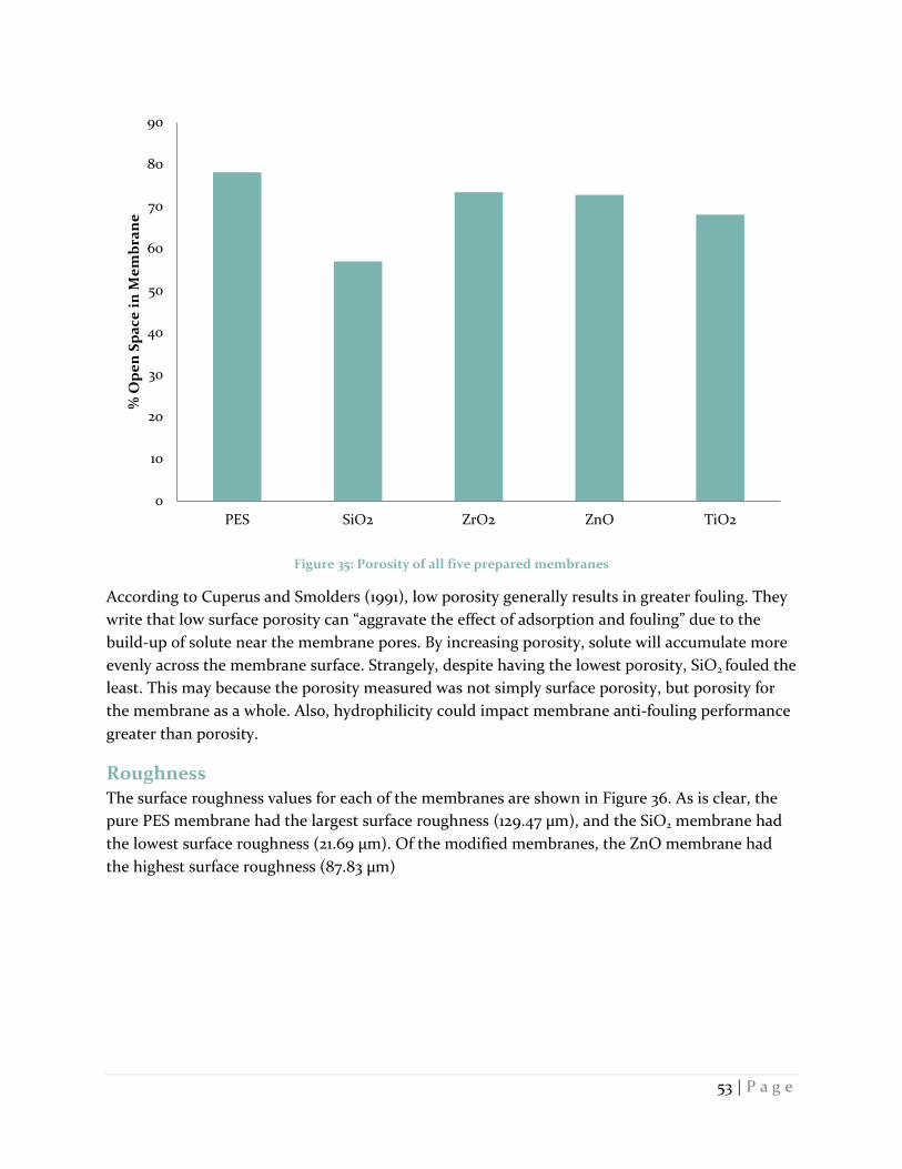
53 | P a g e

Figure 35: Porosity of all five prepared membranes

According to Cuperus and Smolders (1991), low porosity generally results in greater fouling. They

write that low surface porosity can “aggravate the effect of adsorption and fouling” due to the

build-up of solute near the membrane pores. By increasing porosity, solute will accumulate more

evenly across the membrane surface. Strangely, despite having the lowest porosity, SiO2 fouled the

least. This may because the porosity measured was not simply surface porosity, but porosity for

the membrane as a whole. Also, hydrophilicity could impact membrane anti-fouling performance

greater than porosity.

Roughness

The surface roughness values for each of the membranes are shown in Figure 36. As is clear, the

pure PES membrane had the largest surface roughness (129.47 µm), and the SiO2 membrane had

the lowest surface roughness (21.69 µm). Of the modified membranes, the ZnO membrane had

the highest surface roughness (87.83 µm)

0

10

20

30

40

50

60

70

80

90

PES SiO2 ZrO2 ZnO TiO2

% O

pe

n S

pa

ce i

n M

em

bra

ne

54 | P a g e

Figure 36: Roughness values for all five prepared membranes

Greater roughness often results in greater fouling (Cuperus and Smolders, 1991). Greater surface

roughness leads to greater surface area, which creates more opportunities for solute adsorption.

Also, greater roughness “deteriorates” the hydrodynamics near the surface, which in turn

exacerbates concentration polarization as well as fouling. (Cuperus and Smolders, 1991).

Because of this, it is not surprising that the SiO2 membrane had the lowest surface roughness

value, as it was the least susceptible to fouling. Likewise, it is also not surprising that, of the

modified membranes, the ZnO membrane had the highest surface roughness value, as it was the

most susceptible to membrane fouling. Surface roughness, then, could explain why, though the

ZnO membrane was the most hydrophilic, it did not display the best anti-fouling performance.

Mechanical Properties

Mechanical properties of membranes are important to consider as well, and the mechanical

properties of the prepared membranes are shown below. Figure 37 displays the elongation rates of

all five prepared membranes. As is clear, the PES membrane had the best elongation rate, as it was

higher than the four other modified membranes.

0

20

40

60

80

100

120

140

PES SiO2 TiO2 ZnO ZrO2

Ro

ug

ne

ss (μ

m)

55 | P a g e

Figure 37: Elongation rate of the five prepared membranes

Figure 38 displays the breaking force of all five prepared membranes. Again, as is clear, the PES

membrane had the best breaking force, as it was higher than the four other modified membranes.

0

2

4

6

8

10

12

14

16

18

PES PES+SiO2 PES+TiO2 PES+ZnO PES+ZrO2

Pe

rce

nt

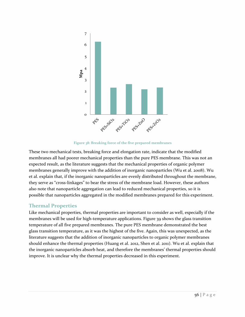
56 | P a g e

Figure 38: Breaking force of the five prepared membranes

These two mechanical tests, breaking force and elongation rate, indicate that the modified

membranes all had poorer mechanical properties than the pure PES membrane. This was not an

expected result, as the literature suggests that the mechanical properties of organic polymer

membranes generally improve with the addition of inorganic nanoparticles (Wu et al. 2008). Wu

et al. explain that, if the inorganic nanoparticles are evenly distributed throughout the membrane,

they serve as “cross-linkages” to bear the stress of the membrane load. However, these authors

also note that nanoparticle aggregation can lead to reduced mechanical properties, so it is

possible that nanoparticles aggregated in the modified membranes prepared for this experiment.

Thermal Properties

Like mechanical properties, thermal properties are important to consider as well, especially if the

membranes will be used for high-temperature applications. Figure 39 shows the glass transition

temperature of all five prepared membranes. The pure PES membrane demonstrated the best

glass transition temperature, as it was the highest of the five. Again, this was unexpected, as the

literature suggests that the addition of inorganic nanoparticles to organic polymer membranes

should enhance the thermal properties (Huang et al. 2012, Shen et al. 2011). Wu et al. explain that

the inorganic nanoparticles absorb heat, and therefore the membranes’ thermal properties should

improve. It is unclear why the thermal properties decreased in this experiment.

0

1

2

3

4

5

6

7

Mp

a

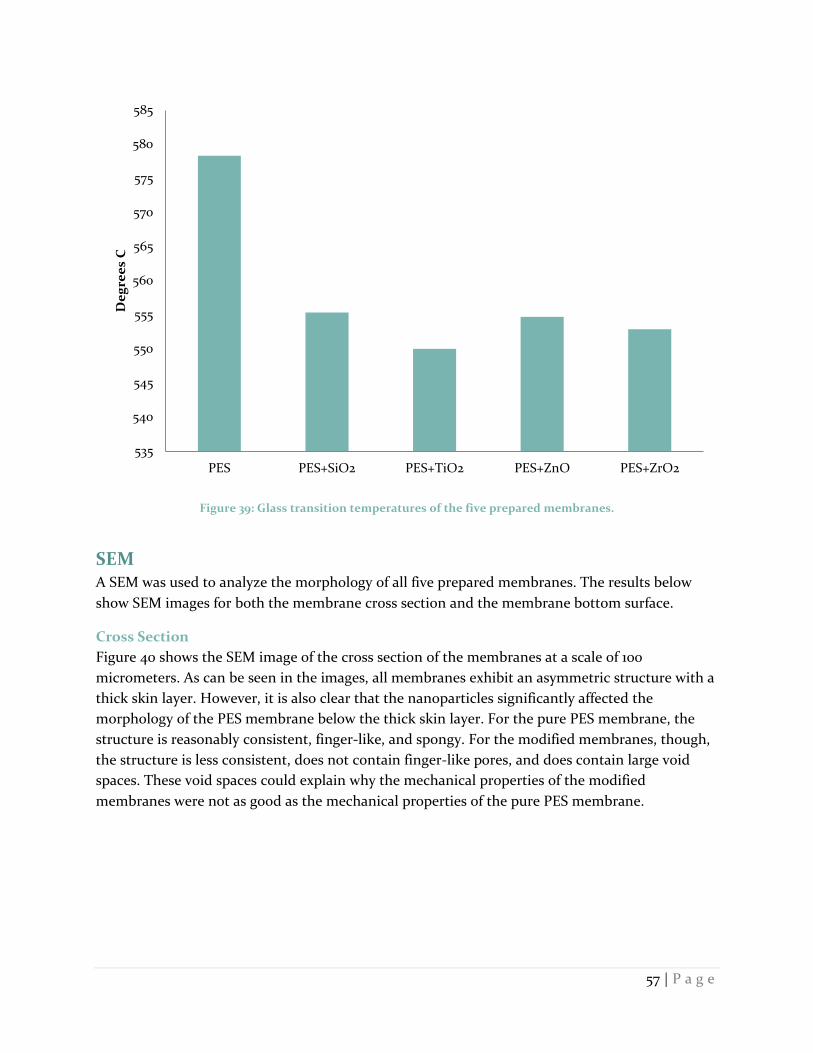
57 | P a g e

Figure 39: Glass transition temperatures of the five prepared membranes.

SEM A SEM was used to analyze the morphology of all five prepared membranes. The results below

show SEM images for both the membrane cross section and the membrane bottom surface.

Cross Section

Figure 40 shows the SEM image of the cross section of the membranes at a scale of 100

micrometers. As can be seen in the images, all membranes exhibit an asymmetric structure with a

thick skin layer. However, it is also clear that the nanoparticles significantly affected the

morphology of the PES membrane below the thick skin layer. For the pure PES membrane, the

structure is reasonably consistent, finger-like, and spongy. For the modified membranes, though,

the structure is less consistent, does not contain finger-like pores, and does contain large void

spaces. These void spaces could explain why the mechanical properties of the modified

membranes were not as good as the mechanical properties of the pure PES membrane.

535

540

545

550

555

560

565

570

575

580

585

PES PES+SiO2 PES+TiO2 PES+ZnO PES+ZrO2

De

gre

es

C

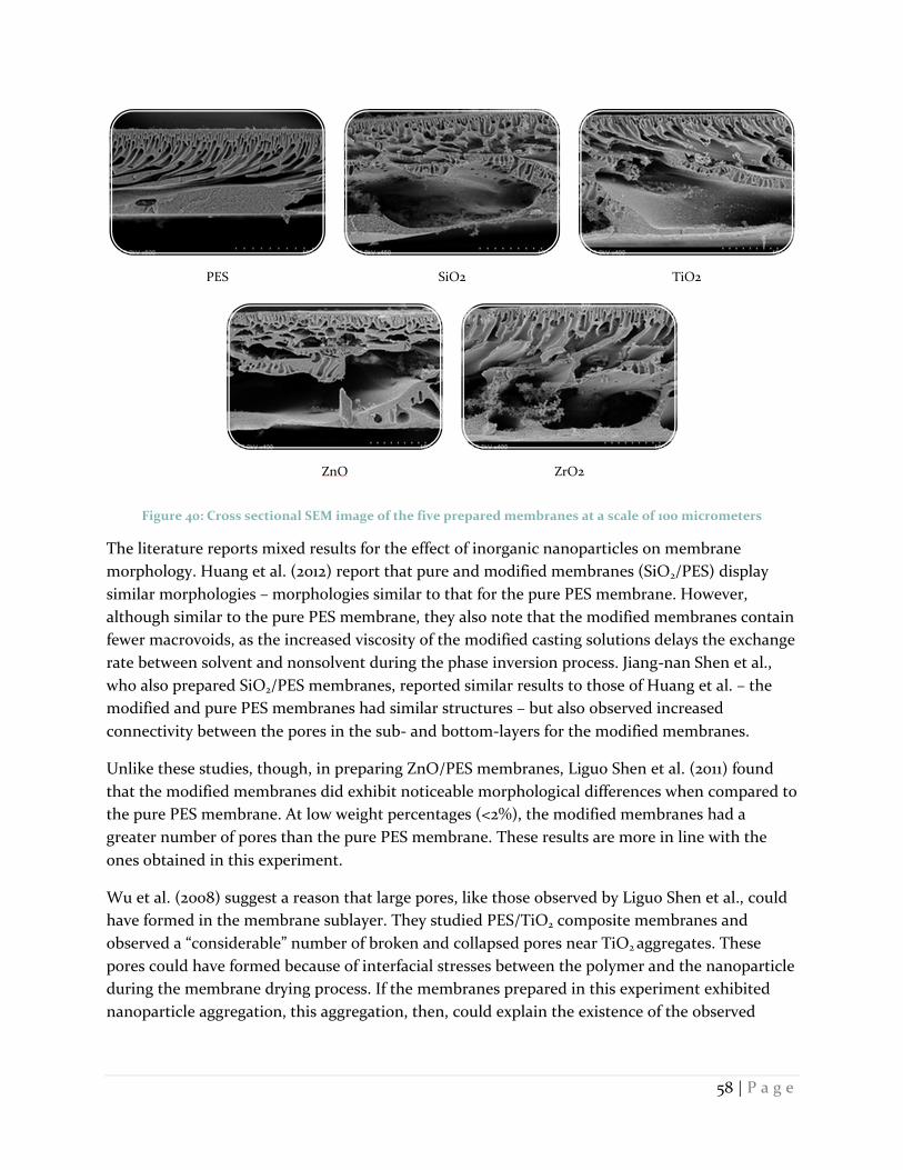
58 | P a g e

Figure 40: Cross sectional SEM image of the five prepared membranes at a scale of 100 micrometers

The literature reports mixed results for the effect of inorganic nanoparticles on membrane

morphology. Huang et al. (2012) report that pure and modified membranes (SiO2/PES) display

similar morphologies – morphologies similar to that for the pure PES membrane. However,

although similar to the pure PES membrane, they also note that the modified membranes contain

fewer macrovoids, as the increased viscosity of the modified casting solutions delays the exchange

rate between solvent and nonsolvent during the phase inversion process. Jiang-nan Shen et al.,

who also prepared SiO2/PES membranes, reported similar results to those of Huang et al. – the

modified and pure PES membranes had similar structures – but also observed increased

connectivity between the pores in the sub- and bottom-layers for the modified membranes.

Unlike these studies, though, in preparing ZnO/PES membranes, Liguo Shen et al. (2011) found

that the modified membranes did exhibit noticeable morphological differences when compared to

the pure PES membrane. At low weight percentages (<2%), the modified membranes had a

greater number of pores than the pure PES membrane. These results are more in line with the

ones obtained in this experiment.

Wu et al. (2008) suggest a reason that large pores, like those observed by Liguo Shen et al., could

have formed in the membrane sublayer. They studied PES/TiO2 composite membranes and

observed a “considerable” number of broken and collapsed pores near TiO2 aggregates. These

pores could have formed because of interfacial stresses between the polymer and the nanoparticle

during the membrane drying process. If the membranes prepared in this experiment exhibited

nanoparticle aggregation, this aggregation, then, could explain the existence of the observed

PES SiO2 TiO2

ZnO ZrO2

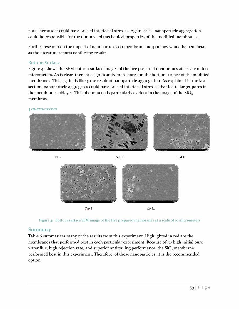
59 | P a g e

pores because it could have caused interfacial stresses. Again, these nanoparticle aggregation

could be responsible for the diminished mechanical properties of the modified membranes.

Further research on the impact of nanoparticles on membrane morphology would be beneficial,

as the literature reports conflicting results.

Bottom Surface

Figure 41 shows the SEM bottom surface images of the five prepared membranes at a scale of ten

micrometers. As is clear, there are significantly more pores on the bottom surface of the modified

membranes. This, again, is likely the result of nanoparticle aggregation. As explained in the last

section, nanoparticle aggregates could have caused interfacial stresses that led to larger pores in

the membrane sublayer. This phenomena is particularly evident in the image of the SiO2

membrane.

5 micrometers

Figure 41: Bottom surface SEM image of the five prepared membranes at a scale of 10 micrometers

Summary Table 6 summarizes many of the results from this experiment. Highlighted in red are the

membranes that performed best in each particular experiment. Because of its high initial pure

water flux, high rejection rate, and superior antifouling performance, the SiO2 membrane

performed best in this experiment. Therefore, of these nanoparticles, it is the recommended

option.

PES SiO2 TiO2

ZnO ZrO2

60 | P a g e

Table 6: Summary of results. The boxes in red indicate the membrane that performed best in each particular category.

61 | P a g e

Recommendations In general, it would be beneficial if research on inorganic nanoparticles and membrane

performance was more systematized. There are numerous different tests, nanoparticles, and

methodologies for preparing and characterizing these composite membranes. As a result, there is

little consistency among experiments conducted in different laboratories, and there is little room

for comparison among different studies. A comprehensive database where researchers from

different labs could input their results according to different methodologies, nanoparticles, and

wt % of nanoparticles, could help solve this problem. This database would also help to make clear

the gaps in knowledge that currently exist and therefore could help to focus future research.

Regarding future research, there are still numerous experiments that could help improve

understanding of the impact inorganic nanoparticles can have on antifouling performance. For

example, in this experiment, the nanoparticles were only dispersed at 1 wt % in the membrane.

Other wt %’s should be tested for all these nanoparticles. Also, due to time constraints, none of

the tests in this experiment were run more than once. Therefore, the membranes prepared in this

study need to be further studied. And last, cleaning methods need to be analyzed, different

wastewaters need to be tested, and economic studies need to be conducted.

To summarize, though this study was one of the first to compare different nanoparticles in

controlled experiments, there still remains significant gaps in knowledge that a more systemized

research strategy would help to fill.

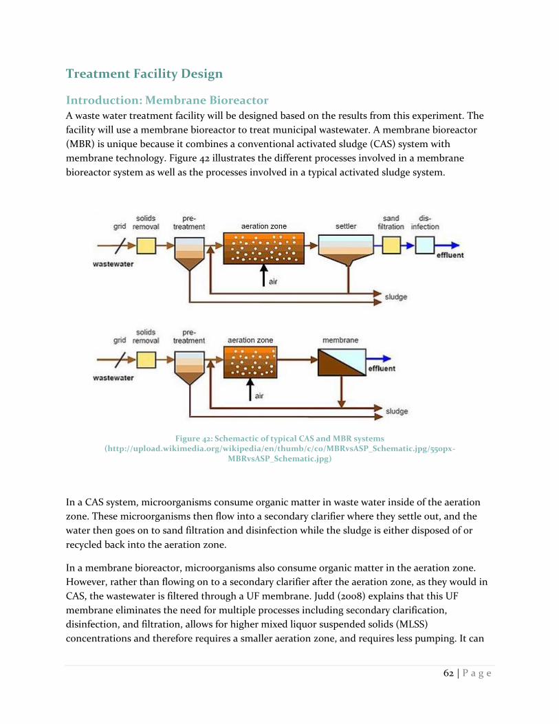
62 | P a g e

Treatment Facility Design

Introduction: Membrane Bioreactor A waste water treatment facility will be designed based on the results from this experiment. The

facility will use a membrane bioreactor to treat municipal wastewater. A membrane bioreactor

(MBR) is unique because it combines a conventional activated sludge (CAS) system with

membrane technology. Figure 42 illustrates the different processes involved in a membrane

bioreactor system as well as the processes involved in a typical activated sludge system.

Figure 42: Schemactic of typical CAS and MBR systems (http://upload.wikimedia.org/wikipedia/en/thumb/c/c0/MBRvsASP_Schematic.jpg/550px-

MBRvsASP_Schematic.jpg)

In a CAS system, microorganisms consume organic matter in waste water inside of the aeration

zone. These microorganisms then flow into a secondary clarifier where they settle out, and the

water then goes on to sand filtration and disinfection while the sludge is either disposed of or

recycled back into the aeration zone.

In a membrane bioreactor, microorganisms also consume organic matter in the aeration zone.

However, rather than flowing on to a secondary clarifier after the aeration zone, as they would in

CAS, the wastewater is filtered through a UF membrane. Judd (2008) explains that this UF

membrane eliminates the need for multiple processes including secondary clarification,

disinfection, and filtration, allows for higher mixed liquor suspended solids (MLSS)

concentrations and therefore requires a smaller aeration zone, and requires less pumping. It can

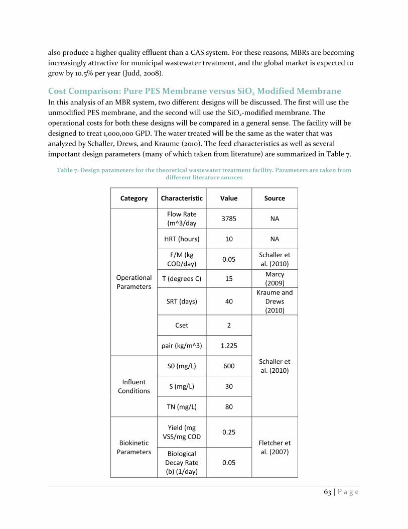
63 | P a g e

also produce a higher quality effluent than a CAS system. For these reasons, MBRs are becoming

increasingly attractive for municipal wastewater treatment, and the global market is expected to

grow by 10.5% per year (Judd, 2008).

Cost Comparison: Pure PES Membrane versus SiO2 Modified Membrane

In this analysis of an MBR system, two different designs will be discussed. The first will use the

unmodified PES membrane, and the second will use the SiO2-modified membrane. The

operational costs for both these designs will be compared in a general sense. The facility will be

designed to treat 1,000,000 GPD. The water treated will be the same as the water that was

analyzed by Schaller, Drews, and Kraume (2010). The feed characteristics as well as several

important design parameters (many of which taken from literature) are summarized in Table 7.

Table 7: Design parameters for the theoretical wastewater treatment facility. Parameters are taken from different literature sources

Category Characteristic Value Source

Operational Parameters

Flow Rate (m^3/day

3785 NA

HRT (hours) 10 NA

F/M (kg COD/day)

0.05 Schaller et al. (2010)

T (degrees C) 15 Marcy (2009)

SRT (days) 40 Kraume and

Drews (2010)

Cset 2

Schaller et al. (2010)

ρair (kg/m^3) 1.225

Influent Conditions

S0 (mg/L) 600

S (mg/L) 30

TN (mg/L) 80

Biokinetic Parameters

Yield (mg VSS/mg COD

0.25

Fletcher et al. (2007) Biological

Decay Rate (b) (1/day)

0.05

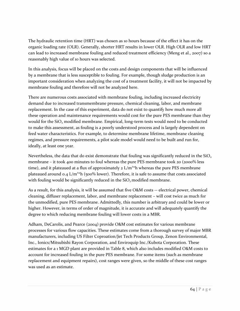
64 | P a g e

The hydraulic retention time (HRT) was chosen as 10 hours because of the effect it has on the

organic loading rate (OLR). Generally, shorter HRT results in lower OLR. High OLR and low HRT

can lead to increased membrane fouling and reduced treatment efficiency (Meng et al., 2007) so a

reasonably high value of 10 hours was selected.

In this analysis, focus will be placed on the costs and design components that will be influenced

by a membrane that is less susceptible to fouling. For example, though sludge production is an

important consideration when analyzing the cost of a treatment facility, it will not be impacted by

membrane fouling and therefore will not be analyzed here.

There are numerous costs associated with membrane fouling, including increased electricity

demand due to increased transmembrane pressure, chemical cleaning, labor, and membrane

replacement. In the case of this experiment, data do not exist to quantify how much more all

these operation and maintenance requirements would cost for the pure PES membrane than they

would for the SiO2 modified membrane. Empirical, long-term tests would need to be conducted

to make this assessment, as fouling is a poorly understood process and is largely dependent on

feed water characteristics. For example, to determine membrane lifetime, membrane cleaning

regimes, and pressure requirements, a pilot scale model would need to be built and run for,

ideally, at least one year.

Nevertheless, the data that do exist demonstrate that fouling was significantly reduced in the SiO2

membrane – it took 400 minutes to foul whereas the pure PES membrane took 20 (2000% less

time), and it plateaued at a flux of approximately 2 L/m2*h whereas the pure PES membrane

plateaued around 0.4 L/m2*h (500% lower). Therefore, it is safe to assume that costs associated

with fouling would be significantly reduced in the SiO2 modified membrane.

As a result, for this analysis, it will be assumed that five O&M costs -- electrical power, chemical

cleaning, diffuser replacement, labor, and membrane replacement – will cost twice as much for

the unmodified, pure PES membrane. Admittedly, this number is arbitrary and could be lower or

higher. However, in terms of order of magnitude, it is accurate and will adequately quantify the

degree to which reducing membrane fouling will lower costs in a MBR.

Adham, DeCarolis, and Pearce (2004) provide O&M cost estimates for various membrane

processes for various flow capacities. These estimates come from a thorough survey of major MBR

manufacturers, including US Filter Coproation/Jet Tech Products Group, Zenon Environmental,

Inc., Ionics/Mitsubishi Rayon Corporation, and Enviroquip Inc./Kubota Corporation. These

estimates for a 1 MGD plant are provided in Table 8, which also includes modified O&M costs to

account for increased fouling in the pure PES membrane. For some items (such as membrane

replacement and equipment repairs), cost ranges were given, so the middle of these cost ranges

was used as an estimate.

65 | P a g e

Table 8: Estimated operating costs for SiO2 and pure PES membranes (based on Adham, DeCarolis and Pearce (2004)

Item

O&M Costs $K/yr

Pure PES Membrane

Plant

SiO2 Membrane

Plant

Electrical Power for Process/Miscellaneous 140 70

Equipment Repairs/Lubricants/Replacement 36 18

Chemical Cleaning 16 8

Chemical Costs for Disinfection 4.6 4.6

Diffuser Replacement 2.4 2.4

Membrane Replacement 100 50

Labor 62 31

Total O&M Costs in First Year 368 184

As is clear from the information in Table 8, operation and maintenance costs, largely due to

fouling, are significant for MBR systems; they are estimated to be $184,000 per year for a small, 1

MGD plant. Therefore, by reducing fouling, the costs of MBR systems will be significantly reduced

as well.

For reference, other design parameters were calculated as well. These calculations are not highly

relevant to the objectives of this experiment but are available nevertheless. They are based on the

recommended design parameters in Table 7, which were taken from various sources.

Excess Sludge

To calculate how much waste sludge the system will produce, it is first important to calculate the

volume of the aeration of the basin. This can be accomplished by using Equation 3 (Marcy, 2009)

(Equation 3)

where V is volume (m3) and Q is flow rate (m3/day).

With this volume, the MLSS concentration within the aeration basin (X) can be calculated using

Equation 4 (Schaller, Drews and Kraume, 2010).

66 | P a g e

(

) (Equation 4)

(

)

With the MLSS concentration, the amount of sludge that is wasted can be calculated using

Equation 5 (Schaller, Drews and Kraume, 2010)

(Equation 5)

Oxygen Demand After calculating ESP, it is possible to calculate the oxygen demand necessary to degrade the

organic matter using Equation 6 (Davis and Masten, 2009). This is important as it will dictate the

amount of aeration necessary for the plant, a large portion of the electricity cost.

(Equation 6)

MO2 is the mass of oxygen required by the system, RCOD is the ratio of COD to BOD in the

wastewater, Ci is the influent COD concentration, and Ce is the effluent COD concentration.

Typically, RCOD is approximately 2.0 (Keipper).

MO2 can be converted to a volumetric flow rate (Qair, theoretical) using the density of oxygen.

However, because the transfer of oxygen is not perfect, QO2 theoretical represents only the theoretical

oxygen demand. According to Fletcher, Mackley and Judd (2007), to determine how much oxygen

must actually be supplied, Equations 7 and 8 must be used.

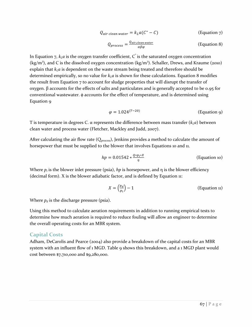
67 | P a g e

(Equation 7)

(Equation 8)

In Equation 7, kLa is the oxygen transfer coefficient, C* is the saturated oxygen concentration

(kg/m3), and C is the dissolved oxygen concentration (kg/m3). Schaller, Drews, and Kraume (2010)

explain that kLa is dependent on the waste stream being treated and therefore should be

determined empirically, so no value for kLa is shown for these calculations. Equation 8 modifies

the result from Equation 7 to account for sludge properties that will disrupt the transfer of

oxygen. β accounts for the effects of salts and particulates and is generally accepted to be 0.95 for

conventional wastewater. ϕ accounts for the effect of temperature, and is determined using

Equation 9

(Equation 9)

T is temperature in degrees C. α represents the difference between mass transfer (kLa) between

clean water and process water (Fletcher, Mackley and Judd, 2007).

After calculating the air flow rate (Qprocess), Jenkins provides a method to calculate the amount of

horsepower that must be supplied to the blower that involves Equations 10 and 11.

(Equation 10)

Where pi is the blower inlet pressure (psia), hp is horsepower, and η is the blower efficiency

(decimal form). X is the blower adiabatic factor, and is defined by Equation 11:

(

) (Equation 11)

Where pd is the discharge pressure (psia).

Using this method to calculate aeration requirements in addition to running empirical tests to

determine how much aeration is required to reduce fouling will allow an engineer to determine

the overall operating costs for an MBR system.

Capital Costs

Adham, DeCarolis and Pearce (2004) also provide a breakdown of the capital costs for an MBR

system with an influent flow of 1 MGD. Table 9 shows this breakdown, and a 1 MGD plant would

cost between $7,710,000 and $9,280,000.

68 | P a g e

Table 9: Breakdown of the capital costs for an MBR system

Item Capital Cost ($K)

Low High

Headworks 450

Basins 484

MBR System 1579 2347

Mechanical 420

Blower and Pump building 247

Chlorine Dosing System 217

Subtotal 3397 4165

Electrical, 15% 510 625

Mechanical/ Plumbing/HVAC, 13% 442 541

Sitework 306 375

Subtotal 4654 5706

Contractor Overhead and Profit, 15% 698 856

Subtotal-Construction Cost 5352 6562

Land 750

Contingency, 15% 803 984

Engineering/Legal/Administration, 15% 803 984

Total Capital Cost 7710 9280

Summary

As demonstrated by Adham, DeCarolis and Pearce (2004), fouling is a significant cost to MBR

processes. By reducing fouling, operational costs reduce as well. The SiO2 membrane prepared in

this experiment fouled significantly less than the unmodified, pure PES membrane (took 20x

longer to foul). However, further empirical tests need to be conducted to determine how much

operational costs would decrease as a result of this enhanced antifouling performance.

Once these empirical tests are complete, the equations provided in the previous sections can be

used to produce a detailed cost estimate for processes such as sludge handling and aeration.

Design parameters taken from the literature and summarized in Table 7 provide all that is

necessary to complete these calculations. Estimates for the capital costs of a 1 MGD plant are

provided in Table 9.

69 | P a g e

References Adham, S., DeCarolis, F., and Pearce, W. (2004). Optimization of Various MBR Systems for Water

Reclamation – Phase III. Desalination and Water Purification Research and Development Report No. 103

Agrawal, A.Wettability, non-wettability and contact angle hysteresis. Retrieved from http://web.mit.edu/nnf/education/wettability/wetting.html Bottino, A., Capannelli, G., & Comite, A. (2002). Preparation and characterization of novel porous PVDF-ZrO2 composite membranes. Desalination, 146(1), 35-40. Choi, J. G., Bae, T. H., Kim, J. H., Tak, T. M., & Randall, A. (2002). The behavior of membrane fouling initiation on the crossflow membrane bioreactor system. Journal of Membrane Science, 203(1), 103-113. Cuperus, F., & Smolders, C. (1991). Characterization of UF membranes: Membrane characteristics

and characterization techniques. Advances in Colloid and Interface Science, 34(2), 135-173. DaRo UV Systems LTD.UV water treatment. Retrieved from http://www.uvwatertreatment.co.uk/images/DNA.jpg

Davis, M. L., & Masten, S. J. (2004). Principles of environmental engineering and science McGraw- Hill New York, NY. DLVO theory image. Retrieved from http://www.malvern.com/labeng/industry/colloids/dlvo_theory_1.jpg Genne, I., Kuypers, S., & Leysen, R. (1996). Effect of the addition of ZrO2 to polysulfone based UF membranes. Journal of Membrane Science, 113(2), 343-350. Goosen, M., Sablani, S., Al‐Hinai, H., Al‐Obeidani, S., Al‐Belushi, R., & Jackson, D. (2005). Fouling

of reverse osmosis and ultrafiltration membranes: A critical review. Separation Science and Technology, 39(10), 2261-2297.

Fletcher, H., Mackley, T., & Judd, S. (2007). The cost of a package plant membrane bioreactor. Water Research, 41(12), 2627-2635. Huang, J., Zhang, K., Wang, K., Xie, Z., Ladewig, B., & Wang, H. (2012). Fabrication of polyethersulfone-mesoporous silica nanocomposite ultrafiltration membranes with antifouling properties. Journal of Membrane Science Jenkins, T. Evaluating and comparing aeration blower power requirements. Wastewater Solutions, Dresser Roots. Jing-Feng Li, J. F., Xu, Z. L., Yang, H., Yu, L. Y., & Liu, M. (2009). Effect of TiO2 nanoparticles on the surface morphology and performance of microporous PES membrane. Applied Surface Science, 255(9), 4725-4732.

70 | P a g e

Judd, S. (2008). The status of membrane bioreactor technology. Trends in Biotechnology, 26(2), 109-116. Kiepper, B. Understanding laboratory wastewater tests: I. organics (BOD, COD, TOC, O&G). CAES Publications Kools, W. F. C. (1998). Membrane formation by phase inversion in multicomponent polymer systems. mechanisms and morphologies Universiteit Twente. Li, J. H., Xu, Y. Y., Zhu, L. P., Wang, J. H., & Du, C. H. (2009). Fabrication and characterization of

a novel TiO2 nanoparticle self-assembly membrane with improved fouling resistance. Journal of Membrane Science, 326(2), 659-666.

Marcy, C. (2009). The Effects of Hydrophobic and Hydrophilic Natural Organic Matter on Charged Ultrafiltration Performance. WPI Major Qualifying Project. Marshall, A., Munro, P., & Trägårdh, G. (1993). The effect of protein fouling in microfiltration and

ultrafiltration on permeate flux, protein retention and selectivity: A literature review. Desalination, 91(1), 65-108.

Matar, O., Hewitt, G., & Ortiz, E.Phase inversion in liquid-liquid dispersions. Department of Chemical Engineering, Imperial College, London Matsuura, T. (1994). Synthetic membranes and membrane separation processes CRC PressI Llc. McCabe, W. L., Smith, J. C., & Harriott, P. (1956). Unit operations of chemical engineering McGraw-Hill Book Company New York. Maximous, N., Nakhla, G., Wan, W., & Wong, K. (2010). Performance of a novel ZrO2/PES membrane for wastewater filtration. Journal of Membrane Science, 352(1), 222-230. Mcintyre, N. (2012, ). How ill climate change impact on fresh water scarcity. The Guardian Membrane structure: SEM images. Retrieved from

http://ars.els-cdn.com/content/image/1-s2.0-S1570023204001345-gr1.jpg

Meng, F., Chae, S. R., Drews, A., Kraume, M., Shin, H. S., & Yang, F. (2009). Recent advances in membrane bioreactors (MBRs): Membrane fouling and membrane material. Water Research, 43(6), 1489-1512. National Geographic (2013). Freshwater Crisis. National Geographic Website. Pereira, L. S., Cordery, I., & Iacovides, I. (2009). Coping with water scarcity: Addressing the

Challenges. Springer. Population Institute (2010). Population and Water. Poyatos, J., Muñio, M., Almecija, M., Torres, J., Hontoria, E., & Osorio, F. (2010). Advanced

oxidation processes for wastewater treatment: State of the art. Water, Air, and Soil Pollution, 205(1-4), 187-204.

71 | P a g e

Queen Mary University of London.5.3 photoelectron spectroscopy. Retrieved from http://www.chem.qmul.ac.uk/surfaces/scc/scat5_3.htm Reihanian, H., Robertson, C., & Michaels, A. (1983). Mechanisms of polarization and fouling of ultrafiltration membranes by proteins. Journal of Membrane Science, 16, 237-258. Saddat, A. (2011). Preparation, characterization and performance optimization of ultrafiltration

membranes produced with polymeric and inorganic additives. ().Worcester Polytechnic Institute.

Schaller, J., Drews, A., & Kraume, M. (2010). Development of a cost model for membrane

bioreactors including sludge handling costs. Desalination and Water Treatment, 18(1-3), 315-320.

Sewerage Business Management Centre.Advanced oxidation process with hydrogen peroxide. Retrieved from http://www.sbmc.or.jp/english/ozonation_technology.files/image002.jpg Shen, J., Ruan, H., Wu, L., & Gao, C. (2011). Preparation and characterization of PES–SiO2 organic– inorganic composite ultrafiltration membrane for raw water pretreatment. Chemical Engineering Journal, 168(3), 1272-1278. Shen, L., Bian, X., Lu, X., Shi, L., Liu, Z., Chen, L., . . . Fan, K. (2012). Preparation and

characterization of ZnO/polyethersulfone (PES) hybrid membranes. Desalination, 293, 21-29

Su, Y., Huang, C., Pan, J., Hsieh, W., & Chu, M. (2011). Fouling mitigation by TiO2 composite

membrane in membrane bioreactors. Journal of Environmental Engineering, 138(3), 344-350.

Turral, H., Burke, J. J., & Faurès, J. (2011). Climate change, water and food security. Food and Agriculture Organization of the United Nations. United States Environmental Protecation Agency. (1999). Wastewater Technology fact sheet: Ultraviolet disinfection United States Environmental Protection Agency. (1999). EPA guidance manual: Chapter 8 ultraviolet radiation., 8-1. Wikipedia. (2010). Contact angle image file. Retrieved from http://en.wikipedia.org/wiki/File:Contact_angle.svg Word Health Organization. (2009). 10 facts about water scarcity. World Water Organization (2010). Water Facts & Water Stories from Across the Globe. Wu, G., Gan, S., Cui, L., & Xu, Y. (2008). Preparation and characterization of PES/TiO2 composite membranes. Applied Surface Science, 254(21), 7080-7086.

72 | P a g e

Xu, Z., Yu, L., & Han, L. (2009). Polymer-nanoinorganic particles composite membranes: A brief overview. Frontiers of Chemical Engineering in China, 3(3), 318-329. Yu, H. Y., Hu, M. X., Xu, Z. K., Wang, J. L., & Wang, S. Y. (2005). Surface modification of polypropylene microporous membranes to improve their antifouling property in MBR: NH3 plasma treatment. Separation and Purification Technology, 45(1), 8-15. Zhou, H., & Smith, D. W. (2002). Advanced technologies in water and wastewater treatment. Journal of Environmental Engineering and Science, 1(4), 247-264.

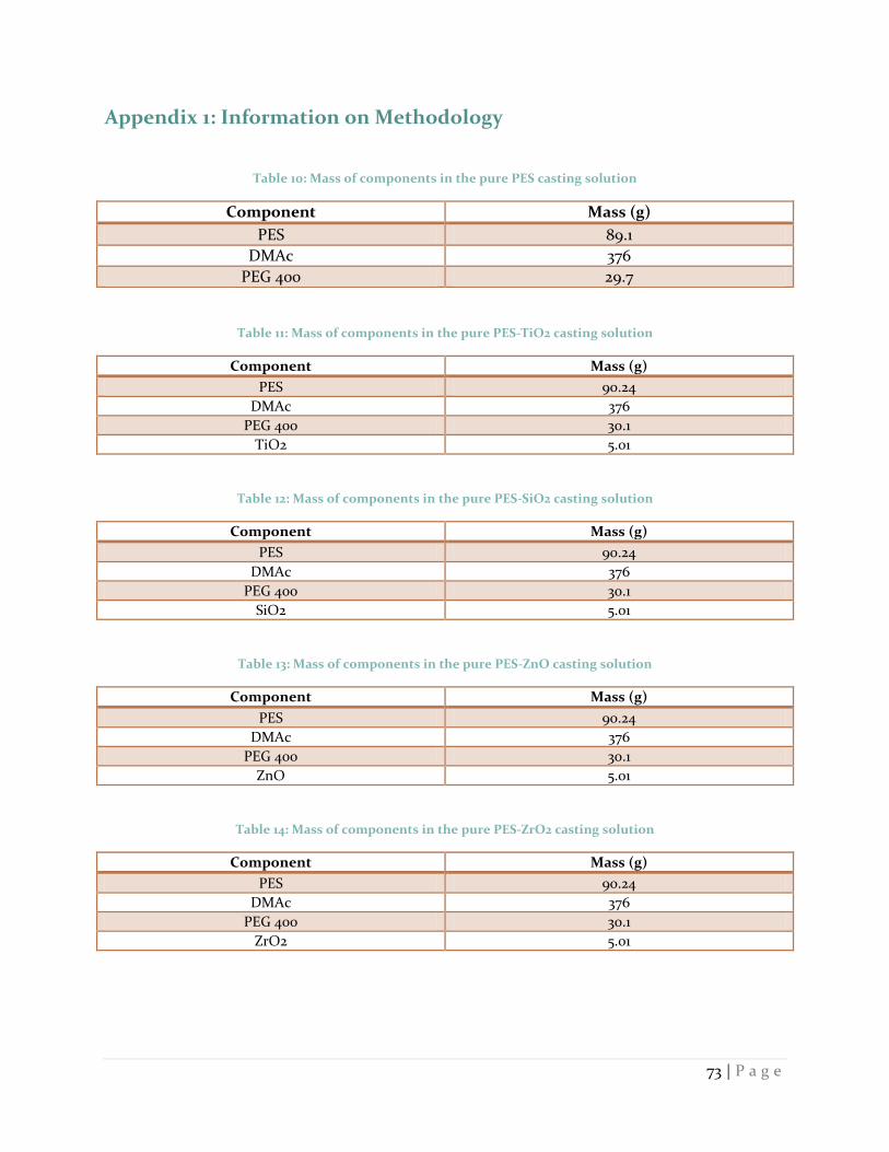
73 | P a g e

Appendix 1: Information on Methodology

Table 10: Mass of components in the pure PES casting solution

Component Mass (g)

PES 89.1

DMAc 376

PEG 400 29.7

Table 11: Mass of components in the pure PES-TiO2 casting solution

Component Mass (g)

PES 90.24

DMAc 376

PEG 400 30.1

TiO2 5.01

Table 12: Mass of components in the pure PES-SiO2 casting solution

Component Mass (g)

PES 90.24

DMAc 376

PEG 400 30.1

SiO2 5.01

Table 13: Mass of components in the pure PES-ZnO casting solution

Component Mass (g)

PES 90.24

DMAc 376

PEG 400 30.1

ZnO 5.01

Table 14: Mass of components in the pure PES-ZrO2 casting solution

Component Mass (g)

PES 90.24

DMAc 376

PEG 400 30.1

ZrO2 5.01

74 | P a g e

Appendix 2: Raw Data

Contact Angle Data Table 15: Contact angle data

Contact Angle

Standard Deviation

% Reduction Contact Angle

PES 67.69 5.44 0

PES+SiO2 62.36 3.92 7.874132073

PES+TiO2 62.05 3.81 8.332102231

PES+ZnO 58.56 4.75 13.48795982

PES+ZrO2 62.53 3.28 7.622987147

Pure Water Flux Data Table 16: Pure water flux of all five membranes before BSA filtration

Time to filter 40g pure H2O no BSA (s)

Mass Flow Rate (g/min)

Mass Flow Rate (g/hr)

Volumetric Flow Rate

(L/hr)

Flux (L*m^-2*hr^-1)

Pure PES 261.02 9.194697724 551.6818635 0.551681863 161.3104864

SiO2 94.17 25.48582351 1529.149411 1.529149411 447.1197107

TiO2 117.33 20.45512657 1227.307594 1.227307594 358.8618696

ZnO 124.22 19.3205603 1159.233618 1.159233618 338.9571982

ZrO2 103.83 23.11470673 1386.882404 1.386882404 405.5211707

Table 17: Pure water flux of pure water directly after BSA filtration

Time to filter 40g pure H2O post BSA filtration (s)

Mass Flow Rate (g/min)

Mass Flow Rate (g/hr)

Volumetric Flow Rate

(L/hr)

Flux (L*m^-2*hr^-1)

Pure PES 2163.49 1.10931874 66.55912438 0.066559124 19.46173227

SiO2 882.81 2.718591769 163.1155062 0.163115506 47.69459245

TiO2 753.02 3.187166344 191.2299806 0.191229981 55.91519901

ZnO 676.95 3.545313539 212.7188123 0.212718812 62.19848313

ZrO2 614.18 3.907649223 234.4589534 0.234458953 68.55524953

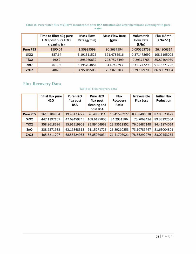
75 | P a g e

Table 18: Pure water flux of all five membranes after BSA filtration and after membrane cleaning with pure water

Time to filter 40g pure H2O post pure H2O

cleaning (s)

Mass Flow Rate (g/min)

Mass Flow Rate (g/hr)

Volumetric Flow Rate

(L/hr)

Flux (L*m^-2*hr^-1)

Pure PES 1590.04 1.50939599 90.5637594 0.090563759 26.4806314

SiO2 387.64 6.191311526 371.4786916 0.371478692 108.6195005

TiO2 490.2 4.895960832 293.7576499 0.29375765 85.89404969

ZnO 461.92 5.195704884 311.742293 0.311742293 91.15271726

ZrO2 484.8 4.95049505 297.029703 0.297029703 86.85079034

Flux Recovery Data Table 19: Flux recovery data

Initial flux pure H2O

Pure H2O flux post

BSA

Pure H2O flux post

cleaning and post BSA

Flux Recovery

Ratio

Irreversible Flux Loss

Initial Flux Reduction

Pure PES 161.3104864 19.46173227 26.4806314 16.41593922 83.58406078 87.93523427

SiO2 447.1197107 47.69459245 108.6195005 24.2931586 75.7068414 89.33292554

TiO2 358.8618696 55.91519901 85.89404969 23.93512852 76.06487148 84.41874054

ZnO 338.9571982 62.19848313 91.15271726 26.89210253 73.10789747 81.65004801

ZrO2 405.5211707 68.55524953 86.85079034 21.41707921 78.58292079 83.09453255

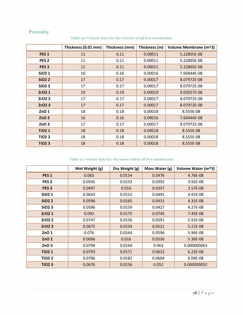
76 | P a g e

Porosity Table 20: Volume data for the exterior of all five membranes

Thickness (0.01 mm) Thickness (mm) Thickness (m) Volume Membrane (m^3)

PES 1 11 0.11 0.00011 5.22805E-08

PES 2 11 0.11 0.00011 5.22805E-08

PES 3 11 0.11 0.00011 5.22805E-08

SiO2 1 16 0.16 0.00016 7.60444E-08

SiO2 2 17 0.17 0.00017 8.07972E-08

SiO2 3 17 0.17 0.00017 8.07972E-08

ZrO2 1 19 0.19 0.00019 9.03027E-08

ZrO2 2 17 0.17 0.00017 8.07972E-08

ZrO2 3 17 0.17 0.00017 8.07972E-08

ZnO 1 18 0.18 0.00018 8.555E-08

ZnO 2 16 0.16 0.00016 7.60444E-08

ZnO 3 17 0.17 0.00017 8.07972E-08

TiO2 1 18 0.18 0.00018 8.555E-08

TiO2 2 18 0.18 0.00018 8.555E-08

TiO2 3 18 0.18 0.00018 8.555E-08

Table 21: Volume data for the water within all five membranes

Wet Weight (g) Dry Weight (g) Mass Water (g) Volume Water (m^3)

PES 1 0.063 0.0154 0.0476 4.76E-08

PES 2 0.0545 0.0153 0.0392 3.92E-08

PES 3 0.0497 0.014 0.0357 3.57E-08

SiO2 1 0.0643 0.0152 0.0491 4.91E-08

SiO2 2 0.0596 0.0165 0.0431 4.31E-08

SiO2 3 0.0586 0.0159 0.0427 4.27E-08

ZrO2 1 0.092 0.0175 0.0745 7.45E-08

ZrO2 2 0.0747 0.0156 0.0591 5.91E-08

ZrO2 3 0.0675 0.0154 0.0521 5.21E-08

ZnO 1 0.076 0.0164 0.0596 5.96E-08

ZnO 2 0.0696 0.016 0.0536 5.36E-08

ZnO 3 0.0794 0.0164 0.063 0.000000063

TiO2 1 0.0793 0.0171 0.0622 6.22E-08

TiO2 2 0.0786 0.0182 0.0604 6.04E-08

TiO2 3 0.0676 0.0156 0.052 0.000000052

77 | P a g e

Table 22: Summary of membrane porosity

Volume Water (m^3)

Volume Membrane (m^3)

Porosity Average Porosity

4.76E-08 5.22805E-08 0.910 0.781

3.92E-08 5.22805E-08 0.750

3.57E-08 5.22805E-08 0.683

4.91E-08 7.60444E-08 0.646 0.569

4.31E-08 8.07972E-08 0.533

4.27E-08 8.07972E-08 0.528

7.45E-08 9.03027E-08 0.825 0.734

5.91E-08 8.07972E-08 0.731

5.21E-08 8.07972E-08 0.645

5.96E-08 8.555E-08 0.697 0.727

5.36E-08 7.60444E-08 0.705

0.000000063 8.07972E-08 0.780

6.22E-08 8.555E-08 0.727 0.680

6.04E-08 8.555E-08 0.706

0.000000052 8.555E-08 0.608

Viscosity Table 23: Viscosity data for the pure PES casting solution

PES

RPM cP %

10 477 15.8

12 483 19.3

20 488 32.6

30 500 50

50 507 84.5

Table 24: Viscosity data for the pure SiO2 casting solution

SiO2

RPM cP %

10 447 14.9

12 450 18

20 459 30.6

30 470 47

50 474 79

78 | P a g e

Table 25: Viscosity data for the TiO2 casting solution

TiO2

RPM cP %

6 560 11.2

10 594 19.8

12 600 24

20 606 40.4

30 618 61.8

Table 26: Viscosity data for the ZnO casting solution

ZnO

RPM cP %

12 527 21.1

20 543 36.2

30 553 55.3

Table 27: Viscosity data for the ZrO2 casting solution

ZrO2

RPM cP %

10 456 15.2

12 463 18.5

20 473 31.5

30 482 48.2

50 487.2 40.4

79 | P a g e

Mechanical Properties

Breaking Force Table 28: Breaking force raw data

BREAKING FORCE (MPa) AVERAGE STDEV

PES 5.8423 6.55688 6.22018 6.27835 6.43263 6.266068 0.27117817

PES+SiO2 2.24217 2.45594 1.98811 2.73231 2.14001 2.311708 0.29014665

PES+TiO2 2.48699 2.69052 1.89974 2.87564 3.11571 2.61372 0.46160649

PES+ZnO 2.04653 2.05077 2.5034 2.01726 2.24855 2.173302 0.20619244

PES+ZrO2 2.09308 2.24038 2.77149 2.19592 2.3208 2.324334 0.26314341

Elongation Rate Table 29: Elongation rate raw data

ELONGATION RATE (%) AVERAGE STDEV

PES 11.6305 15.3347 12.5917 21.8507 20.0742 16.29636 4.51503912

PES+SiO2 6.25809 10.1861 8.92578 10.9996 7.44431 8.762776 1.94085082

PES+TiO2 6.22101 6.51836 4.29658 10.0363 17.2956 8.87357 5.1433077

PES+ZnO 9.51747 5.62978 8.2972 8.18476 8.26013 7.977868 1.42375741

PES+ZrO2 8.85111 7.07436 8.77764 9.11111 9.62845 8.688534 0.96202145

80 | P a g e

Appendix 3: Calibration Curves Table 30: Data for BSA calibration curve

Concentration (mg/L) Absorbance

0 0

10 0.014

100 0.071

200 0.129

400 0.244

700 0.442

1000 0.637

Figure 43: BSA calibration curve, which was generated using the data in Table _

y = 0.0006x + 0.0029 R² = 0.9994

0

0.1

0.2

0.3

0.4

0.5

0.6

0.7

-500 0 500 1000 1500

Series1

Linear (Series1)