PRELIMINARY STUDY ON SST FORECAST SKILL … · RESUME Une nude anterieure de Rosati et al. (IY55) a opine que la previ.\ion du El Nino

$Page 1: PRELIMINARY STUDY ON SST FORECAST SKILL … · RESUME Une nude anterieure de Rosati et al. (IY55) a opine que la previ.\ion du El Nino$
PRELIMINARY STUDY

ON SST FORECAST

SKILL ASSOCIATED

WITH THE 1982/83 EL

NINO PROCESS, USING

COUPLED MODEL

K.Miyakoda,J. PloshayandA. Rosati DATA ASSIMILATION

Reprinted from

ATMOSPHERE-OCEAN SPECIALVol. XXXV, No.1, pp. 469-486March, 1997

')

PRINTED IN CANADA

Preliminary Study on SST Forecast SkillAssociated with the 1982/83 EI Nino Process,

Using Coupled Model Data Assimilation

K. Miyakoda, J. Ploshay and A. RosatiGFDUNOAA Princeton University,

Princeton, NJ 08542, U.S.A.

[Original manuscript received I May 1995; in revised form 22 August 1995]

ABSTRACf A previous study by Rosati et al. (1997) has concluded that the specificationof an adequate thermocline structure along the equatorial Pacific ocean is most crucial

for El Nino forecasts. In that paper, the oceanic initial condition was generated by a dataassimilation (DA) system (Derber and Rosati, 1989). However, the initial condition for theatmospheric part was taken from the National Meteorological Center's (NMC) operational

-analysis, which was simply attached to the oceanic part for the coupled model forecasts.In the present paper, both the atmospheric and oceanic initial conditions are generated

by a coupled DA system applied to a coupled air-sea general circulation model (GCM). Theassimilation for the ocean is performed by the same system as mentioned above, in which theSST (sea surface temperature) and the subsurface temperatures are injected into a 15 verticallevel oceanic GCM. The upper boundary condition, such as surface wind stress, is specifiedby the atmospheric DA. The assimilation for the atmosphere is performed by the continuousinjection method of Stern and Ploshay (1992), using an 18 vertical level atmospheric GCM.The lower boundary condition, such as SST, is specified by the oceanic DA. The coupledmodel assimilations are carried out by switching the DA processes alternately every 6 hoursbetween the ocean and the atmosphere.

The emphases of this study are: firstly, the effect of coupled air-sea model DA on theperformance of sub$equent forecasts; secondly, the impact of the coupled assimilation onimprovement of the "spin-up" behaviour of forecasts, i.e. to see whether a smooth startto the forecast is achieved by the coupled model DA process; and thirdly, investigationof the effect that the "spring barrier" has on predictability in the coupled GCM system.Preliminary results indicate that, in order to answer these questions. ensemble forecasts arenecessary. Besides, the coupled assimilation could be important in improving the overallbehaviour of El Nino and La Nina forecasts.

RESUME Une nude anterieure de Rosati et al. (IY55) a opine que la previ.\ion du El Ninodepend grandement de la .I'pecification d'une .I'tructure thermocline adequate .I'ur l'oceanPacifique equatorial. Dan.1' cette nude. la condition initiale oceanique utilisait Ie sy.l'temed'a.I'.l'imilation de.1' donnee.1' (DA) de Derber et Ro.l'ati (IY8Y). Tout~foi.l'. la condition initialede la partie atmo.\pherique nait constituee de l'analY.l'e reguliere du NMC (National Mete-orological center) qui nait .I'implement rattachee a la partie oceanique pour les previsionsdu modele couple.

470/ K. Miyakoda, J. Ploshay and A. Rosati

Ici les conditions initiales, rant atmospheriques qu'oceaniques, sont generees par unsysteme DA couple applique a un modele de circulation generale (GCM) couple air-mer.L 'assimilation pour l'ocean est effectuee par Ie meme systeme que ci-dessus, dans lequellatemperature superficielle de la mer (SST) et les temperatures sous la surface sont injecteesdans un GCM oceanique a 15 niveaux verticaux. La condition a la couche limite superieure,p. ex. la force d'entramement du vent de surface, est determinee par Ie systeme DA at-mospherique. L 'assimilation pour l'atmosphere est accomplie par la methode d'injectioncontinue de Stem et Ploshay (1992), utilisant un GCM atmospherique de 18 niveaux verti-caux. Les conditions a la limite inferieure, telle que la SST, sont determinees par Ie systemeDA oceanique. Les assimilations du modele couple sont effectuees en enclenchant altema-tivement les processus d'assimilation de l'ocean et de l'atmosphere a routes les six heures.

L 'etude porte surtout sur: l'effet du modele avec systeme DA couple air-mer sur la per- "formance des previsions subsequentes.. I 'impact de l'assimilation couplee sur I 'ameliorationdu comportement de depart des previsions (p. ex., un depart doux de la prevision resulte-t'ildu systeme DA du modele couple) ..l'investigation de l'effet que la «barriere printanniere»a sur la prevision dans Ie systeme de GCM couple. Les premiers resultats indiquent que .des previsions d'ensembles sont necessaires afin de repondre a ces questions. En outre,l'assimilation couplee pourrait etre importante pour ameliorer Ie comportement general dela prevision du EI Nino et de LA Nina.

1 IntroductionTropical oceanic-atmospheric forecasts have been considerably improved, usingsimple dynamical models or statistical methods (see Barnett et al., 1988). In thispaper, however, the approach will be exclusively based on the coupled atmosphere-ocean general circulation models (GCMs). The issue is the seasonal forecasts, whichtreat the global oceanic and atmospheric states on the time ranges ,of about one

year.Concerning the activities related to the low frequency variation of the atmosphere,

it is known (see for example, Brankovic et al., 1994) that the El Nino/SouthernOscillation signal is most dominant. This suggests that the forecast of ENSO shouldbe of greatest concern in order to unravel the possibility of seasonal forecasting,and thereafter, further search for predictable elements should be pursued over otherareas uf the globe.

The simple model approach for El Nino prediction, such as Cane and Zebiak(1985) and Cane et ill. (1986), treats the anomaly components of variables. Onthe other hand, the GCM approach has to treat the total components. This aspectpresents one of the difficult and yet challenging problems in forecasts. An exampleis obtaining a good seasonal cycle of SST in the eastern equatorial Pacific, i.e.,NINO-3 (1500W-90oW, 5°N-5°S) region, which is a formidable task. Accordingto GCM experience (see for example, Neelin et al., 1992; Miyakoda et al., 1993), .the coupling process is extraordinarily sensitive to the character of the atmosphericpart of the physics and orographic or coast-line specifications.

Rosati et ill. (1997) have shown successful forecasts, using a coupled oceanic-atmospheric GCM. The results are very encouraging. However, there are several

SST Forecast Skill Associated with the 1982/83 EI Nino Process /471

issues that have to be made clear. They are: the limit of predictability, the spring bar-rier and the reduction of forecast errors associated with the initial spin-up problem.In order to investigate these issues, ensemble forecasts are useful or even required.If so, an adequate scheme for constructing the initial condition is essential. Themain objective of this paper is to describe a DA system with a coupled oceanic-atmospheric GCM.

2 Background

Rosati et al. (1996) reported the results of 13-month forecasts, using a coupledatmospheric-oceanic GCM with fine equatorial resolution.

a ModelThe atmospheric part has spectral triangular truncation at zonal wavenumber 30,corresponding to 4.0° longitude x 4.0° latitude (see Laprise, 1993) and 18 verticallevels. On the other hand, the oceanic part has a 1 ° x 1 ° longitudinal and meridional

resolution outside of 100N-100S and 1/3° inside of the equatorial zone (Philanderand Seigel, 1985). A set of adequate subgrid-scale physics for the atmosphere andocean model is included. The prediction domain is the entire global atmosphereand the world ocean between 65°N and the Antarctic. All forecasts in this paperdo not include flux corrections (Sausen et al., 1988).

The atmosphere and ocean models are coupled by exchanging the fluxes ofmomentum, heat, radiation and the SST specification with each other.

b Initial conditionsThe inclusion of adequate information in the initial conditions is of considerableimportance for weather forecasts; it may also be true for seasonal forecasts.

As the first step toward coupled model prediction, a scheme of oceanographicDA was developed by Derber and Rosati (1989). This was based on the variationalmethod, in which various constraints are included to specify dynamical formulaeand observational accuracies. Through these constraints, the observed SST and sub-surface data, XBT (expendable bathythermograph) and others, are injected into theocean model through the optimum interpolation scheme (01). The upper boundaryconditions of the ocean GCM are specified by surface wind stress, atmosphericheat flux, moisture flux and incoming shortwave and net longwave radiation. Mostof these data are taken from the NMC (National Meteorological Center) opera-tional analysis, with the exception that the radiation is given by the seasonallyvarying climatologies. The ocean model is integrated forward in time for manyyears (1979-1988), while these data are continuously injected and assimilated intothe model (see Rosati et al., 1995 for more detail).

c CasesThe forecast cases consist of 7 episodes starting from January or July every yearfor the 7 years of 1982-1988. During this 7-year period, there are two distinct El


.January cases

DC

-2 .

-3

82 83 84 85 86 87 88

1.

.7

.2

-.2

-.7

82 83 84 85 86 87 88 89

Fig. 1 Perfonnance of the 13-month forecasts is shown by SST anomalies for NINO-3 region (upper)and ENSO indices; i.e. ESJ (lower). Thick curves are the observations, and the curves connected

with crosses are the forecasts (after Rosati et al., 1997).

Nino events and two events of La Nina. The initial condition time is 0000 GMT onthe first day of January or July. The time range of the forecasts is 13 months.

d Prediction skillThe results of the 7 January forecasts are displayed in Fig. I. For each month of theforecasts, the monthly mean SST anomaly was computed over the NINO-3 regionand is shown in the upper panels. The lower panel is the zonal mean heat contentanomaly index or ENSO index, i.e. ESI, which will be explained below.

For the atmosphere alone, the SOl (Southern Oscillation Index) is a traditional


indicator of the low-frequency atmospheric oscillation, which operates over thesemi-global domain (Troup, 1965; Trenberth, 1976). On the other hand, for thecoupled system, other indices appear to be more appropriate. The first measureis of the west-east tilt of the 20° isotherm along the equatorial Pacific, which isdefined by

GRD = (Dw -D~)/110 -1 (1)

where D is the depth of the 20° isotherm, and Dw and D~ are its depths at 1600Eand 9O0W respectively. The mean value of Dw -D~ is 110 metres, i.e. 160 -50 =110. When GRD is negative, the situation corresponds to the warm phase in theeastern tropical Pacific, i.e. El Nino, while when the GRD is positive, the situationcorresponds to the cold phase, i.e. La Nina.

In order to eliminate the seasonality of the DA, the anomaly of GRD is calculated,in a similar way as for the SOl. This anomaly is referred to as the ENSO index,or simply ESI, i.e.

ESI = GRD -GRD (2)

where GRD is the average over multiple years for the respective month, and it is,therefore, a function of Julian day (or month).

The continuous thick line curves in Fig. 1 are observed SST anomalies for theNINO-3 region (upper panel), after Reynolds (1988), and the ESI from the DA(lower panel). The thin line curves with crosses are the SST and ESI anomaliesfrom the 7 forecast cases, each run for 13 months. The terminal points of the 13-month forecasts are indicated by black dots with crosses. Although the forecastsstarted from the DA, the first month does not agree exactly, because it is a monthlymean of the forecast.

The SST forecasts, shown in the upper panel, agree quite well with the obser-vations, capturing the temperature increases in 1982/83 and 1986/87 and also thetemperature decreases in 1983/84 and 1987/88. During 1984/85 when the anoma-lies had little change the forecasts again did well. The lower panel is the ESI andit should be noted how well it correlates with the NINO-3 SST anomaly. The fore-casted ESI seems to capture the anomalous behaviour of the heat content associatedwith the rise and fall of the thermocline and hence yields a good SST prediction.

An additional measure is "the zonal mean of thermocline anomalies" (Li, per-sonal communication), as opposed to the gradient of the thermocline anomalies,i.e. ESI. The second measure is of the zonal mean of the 20°C isotherm along theequatorial Pacific, which is defined by

MEAN = (Dw + DE)/210 (3)

where 210 = 160 + 50 see (1). In order to eliminate the seasonality, the anomalyof MEAN is calculated. This anomaly is referred to here as the memory index.

memory index = MEAN -MEAN (4)


SST Anomaly Correlation NINO 31.0

.9

.8

", -~-'I.~ _-0+ >+ "- ,~- ,.7 , ,, JUL

"" I.8 \,/

,,.5 ,\

\\

.4 \\\\

.3 '.

\

PERSISTENCE '..2 (Jan) '.

\\\

.1 ~,,,,0 '

-.1 months

-.2

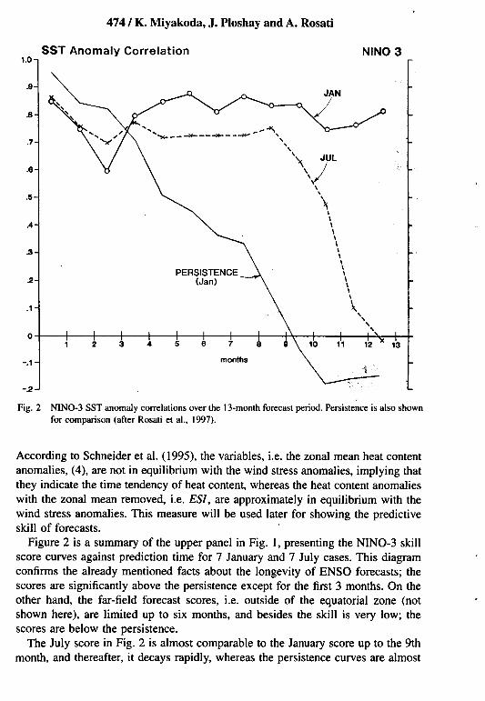
Fig. 2 NINO-3 SST anomaly correlations over the] 3-month forecast period. Persistence is also shownfor comparison (after Rosati et a]., ]997).

According to Schneider et al. (1995), the variables, i.e. the zonal mean heat contentanomalies, (4), are not in equilibrium with the wind stress anomalies, implying thatthey indicate the time tendency of heat content, whereas the heat content anomalieswith the zonal mean removed, i.e. ESl, are approximately in equilibrium with thewind stress anomalies. This measure will be used later for showing the predictiveskill of forecasts.

Figure 2 is a summary of the upper panel in Fig. I, presenting the NINO-3 skillscore curves against prediction time for 7 January and 7 July cases. This diagramconfirms the already mentioned facts about the longevity of ENSO forecasts; thescores are significantly above the persistence except for the first 3 months. On theother hand, the far-field forecast scores, i.e. outside of the equatorial zone (not .

shown here), are limited up to six months, and besides the skill is very low; thescores are below the persistence.

The July score in Fig. 2 is almost comparable to the January score up to the 9thmonth, and thereafter, it decays rapidly, whereas the persistence curves are almost


the same for both the January and July cases. It may be worth noting that the scoresare worse than persistence in the first 3 months, and that this feature is very similarboth in the January and July cases.

3 Issues on forecast skillThere are a number of issues related to the ENSO forecasts. The subjects weare interested in here are: Forecast error growth, Spring barrier, and Initial dip offorecast skill.

a Forecast error growthAccording to some model-twin experiments (Gent and Tribbia, 1993), if initialperturbations are given to the vertical temperature distribution of the ocean, the SSTerror increases rapidly, for example, from 10-40c to 10-loC in about two weeks,and as a result, the correlation coefficients (15°N-15°S Pacific basin) drop to 0.5after 4.5 months. This degree of error growth is normally inevitable, and is knownas predictability decay. On the other hand, the correlation curves in Fig. 2 decaymore slowly than those of Gent and Tribbia. The reason for the high correlationin Fig. 2 may be the fact that El Nino and La Nina forecasts are included, andthat the successful forecasts of these extreme events have contributed to raising theforecast skill curves higher than that of Gent and Tribbia.

b Spring barrierIt has been argued, based on the Cane-Zebiak model (Cane and Zebiak, 1985),that there is a "prediction barrier" in the spring season and, as a consequence, thatthe forecasts starting from January are worse than those from July (see Zebiak andCane, 1987; Blumenthal, 1991; Latif and Graham, 1991; Goswarni and Shukla,1993), though the view has recently been revised (Dr. Busalacchi, personal com-munication). Webster and Yang (1992) also show, from the lag-lead correlationsof the SOl, that May and April emerge as the discontinuity season. As Balmasedaet al. (1994) mentioned, based on the analysis of their simple model forecasts,the correlation skill shows a pronounced drop during spring, often followed by arecovery, due to its memory of the ocean heat content. In other words, the infor-mation from the heat content and SST is not lost simultaneously. Comparing theforecasts between the January and July cases in Fig. 2, it appears that the skillscore is higher in the January than in the July cases, and that the July score dropsin April. However, the sample number in Fig. 2 is too limited to confirm the barrierissue.

c Initial dip of forecast skillIn Fig. 2, an inferior performance is evident in the first 3 months. Two possiblecauses can be considered. One is the "climate drift", because of the model's biascompared with the truth. Another is the improper adjustment of the initial conditionto the model's climatology.


The first issue is outside of the scope of the present paper. Concerning thesecond issue, it appears that a substantial improvement of the initial data andits initialization is desired, perhaps including the precursor of the westerly burstsappropriately (Luther et al., 1983), and refining the model's interactive cloudsproperly (Gent and Tribbia, 1993). This inferior performance is a definite drawbackin the current scheme of Rosati et al. (1997). Investigation should be made as towhat extent the coupled model DA can improve this spin-up behaviour.

4 Data assimilation for the coupled system

In order to improve the spin-up problem, and facilitate the ensemble forecasts,a system of data assimilation is developed for the coupled atmospheric-oceanicmodel.

a Schemes of the coupled model DAThe oceanic DA was described in Section 2. The level II oceanic data are: COADS(Comprehensive Ocean Atmospheric Data Set), MOODS (Master Ocean Observa-tion Data Set), NODC (the National Oceanic Data Center), and TOGA (TropicalOcean and Global Atmosphere Project), which proviqe the data of surface oceantemperature and the vertical temperature profiles through the XBT.

The atmospheric DA is also based on a continuous injection method but in adifferent way (Stem and Ploshay, 1992). Level II meteorological data, such asradiosonde measurements, satellite soundings, aircraft reports, etc., are assimilatedinto the atmospheric GCM, where these data are injected continuously throughthe 01 scheme into the atmospheric model with the help of linear normal modeinitialization (Daley and Puri, 1980). In this process, the observed data are treatedby taking only the incremental part beyond the first guess, i.e. forecast, and applyingthe increments to the linear balance in the multivariate framework. This atmosphericsystem and the resulting analyses have proven to be of comparable accuracy to thoseof operational centres in 1985 (Ploshay et aI., 1992).

In particular, it is a salient feature of this continuous scheme that the initialcondition does not produce any spin-up or spin-down effect. On the other hand, theintermittent scheme produces this transient character through the non-linear normalmode initialization, though there has been an effort to reduce this deficiency byintroducing non-adiabatic effects (Wergen, 1987).

Using these continuous DA schemes of atmosphere and ocean, two systems ofcoupled model DA are developed.

1 THE FIRST COUPLED DA

The assimilation is performed through switching the DA for the ocean and theatmosphere alternately at a 6-hour interval. Namely the atmospheric DA is run for6 hours by inserting the level II meteorological data. The 6-hour averages of windstress, heat fluxes, and long and short wave incoming radiation are saved to forcethe ocean model. The ocean model is then run for 6 hours by inserting the level II


oceanographic data, and returns the 6-hour averages of SST to be used during thenext 6 hours by the atmospheric model.

This coupled DA method requires a 20% increase in computer memory abovecoupled forecasts. The technical difficulty was to set up the switching processbetween the atmosphere and the ocean DA. In any event, this technique has beencompleted and tested successfully. The computer time for the coupled DA is aboutthree times that for the coupled simulation.

2 THE SECOND COUPLED DA

In order to quickly see the effect of coupled DA, a different method was also tested.Using the same DA systems of the atmosphere and the ocean, described under thefirst coupled DA, the oceanic and the atmospheric DA were processed separatelyfor 10 days, and this separate process was iterated twice. The computer time istherefore twice that for the coupled simulation.

b Results of the DAsThe coupled model DAs were applied to construct the 1982 initial conditions.The DA process for the coupled system was started at 10 dayS before 0000 GMT1 January 1982. However, the oceanic DA alone had already been run from 1979.

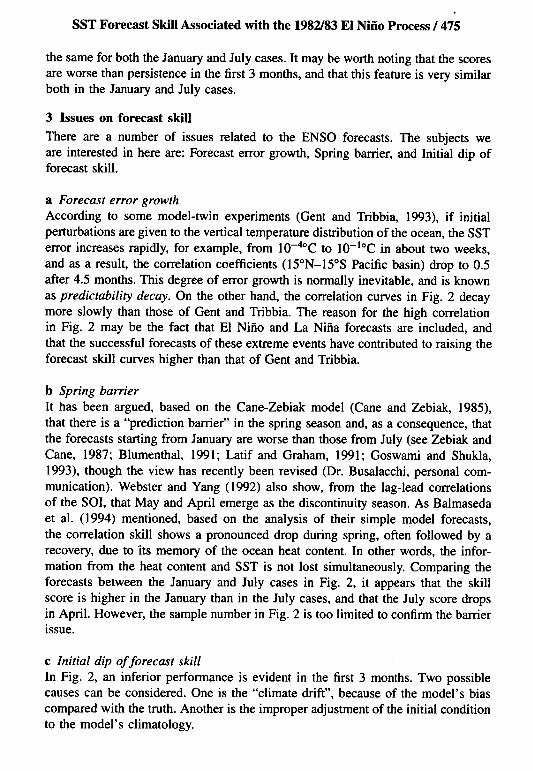
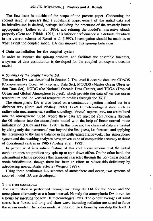
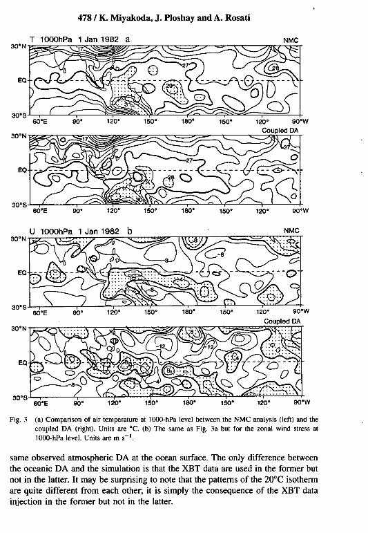
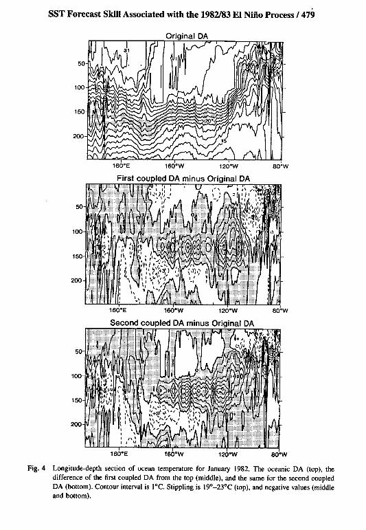
Figures 3a, 3b and 4 show the comparison of resulting atmospheric analysis be-tween the NMC's DA and the coupled model DAs (the first version). The variablesare temperature (Fig. 3a) and the zonal wind at the lOOO-hPa level (Fig. 3b). Thereis a tendency for the zonal wind in the coupled DA to be more intense than those ofNMC. Figure 4 shows the vertical sections of ocean temperature along the equator,which delineate the thermocline structure in the Pacific. In January 1982, there isalready a tendency for the eastern part of the thermocline to be depressed. The toppanel is based on the observed atmospheric forcing of the NMC analysis, whichis the original DA (Rosati et al., 1995). The middle panel is the result of the firstcoupled model DA, and the bottom panel is that of the second coupled DA. Thedifference between the first and the second method is very subtle. The thermoclines(20°C isotherm, for example) are shallower at around 120oW in the coupled DAthan in the original DA (top). Furthermore, the second version (bottom) is evenshallower than the first version, implying that the structure is more adjusted to thethermocline climatology of this particular coupled model.

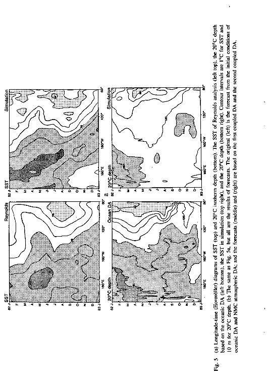
It is customarily considered that one of the best ways to evaluate the DA productsis to utilize them for forecasts. Using these analyses, 13-month forecasts werecarried out. Figures 5a and 5b are Hovmoller (longitude-time) diagrams representingthe time evolution of the SST (top), and the depth of 20°C isotherms (bottom).Among them, Fig. 5a does not show forecasts, but the oceanic DA (left), and theocean simulation (right). The SST fields (left top) are based on Reynolds (1988),and the 20°C isotherm depth (left bottom) is based on Rosati et al. (1995). On theother hand, the top and bottom of the right hand side figures show the results ofocean simulation. Both the ocean DA and simulation are performed by forcing the


T 1000hPa 1 n 198230.N

EO

30.SGO.E 90. 120. 150. 180. 150. 120. 9O.W

30.N

EO

30.SGO.E 90. 120. 150. 180. 150. 120. 90.W

NMC30.N

EO

30.S GO.E 90.

30.N

EO

30.S GO.E 90. 120. 150. 180. 150. 120.

Fig. 3 (a) Comparison of air temperature at IOOO-hPa level between the NMC analysis (left) and thecoupled DA (right). Units are °C. (b) The same as Fig. 3a but for the zonal wind stress atIOOO-hPa level. Units are m s-i.

same observed atmospheric DA at the ocean surface. The only difference betweenthe oceanic DA and the simulation is that the XBT data are used in the former butnot in the latter. It may be surprising to note that the patterns of the 20°C isothermare quite different from each other; it is simply the consequence of the XBT datainjection in the former but not in the latter.

SST Forecast Skill Associated with the 1982/83 El Nino Process / 479

5

1

1

200

First coupled DA minus Original DA

100

1

200

160.E 1 1

Second cou led DA minus Ori inal DA

50

100

150

200

c

160.E 160.W 120.W SO.W

Fig.4 Longitude-depth section of ocean temperature for January 1982. The oceanic DA (top), thedifference of the first coupled DA from the top (middle), and the same for the second coupledDA (bottom). Contour interval is laC. Stippling is 19°-23°C (top), and negative values (middleand bottom).

.c ." ...0-=

&~'"

"'E-6u cn .-

0 cn.~..(0.."'0N.26" U u"'g.c ~--0 ~ 0.

~-;::: .~ 0-"=0 u-~ .".::: '" " =,,~.:;o~ t 6 ij.~ ~ 0 '"'" = ol: ">. .-.c

~ ~ ~ ."~ 8 u §'" = ~

" 0 0 <ou"-O= .">.Z'.c."".c-"~oo",- 0.

..." ~06£8E-O~-cn~~~

cnO_~

.0 ~

"~=,,.= .c .-.cE- -.~ -

.0. 0..=~" 06 ." "

8u,="'g-0 E- ~j,~.,;.o;,,~~-.c ..~

I- 0.--(/) ".,,~Z'(/) ." = .~ .c~-oo

~ < Z Q~~~ i 5,::;"5"5-

.c.c",."_00-=0.1:: -~

'" ~

.-0. '" ~

uo~~0 -:::-,,'"~=.c:2" 0 -E." .~ P! ~= ~ to '"~- -~ -'"~E~~0..- u0 '" -~

-:::- = ~ 0E- .-.0 ..-cnE-tU"cncn-r..:;...cn .."0 " .~ =",.c~~6 -.'" <-

EE~O00 0 ".~ ~ E .~." 0 ~ ~

.0 '" "~ .c

~.:::"o.-",=",

0 ;0-,",0E~~6><e.~

~ ..0 Z Q" ~,,-, < 0 Z ~O .U~ ~ ~ ~ .~ .:; ~

"§&Z6 " .".;;: g u -g" 0 ~""'0 ~.cN .~ -..0

00 = 0c 0..- u

.3 ] 6 .~

'2~ou~.o-o-r.

00~

2 2

~ ~

~ ~~ ~

w w~ 2~ --

C"Oz~ ~ ~ ~

2 2

"2 "2 .--~ ....c :]

~~ ~ ~~ ~--Or)

00~w w2 2--.

C"Oz~ ~ ~ ~

2

~

~.~

w

~

~ ~ ~ ~

482 I K. Miyakoda, J. Ploshay and A. Rosati

Figure 5b shows the three forecasts. These results are compared with those of Fig.5a. The forecast at the left is the same as that of Rosati et al. (1996), which is basedon the NMC and the oceanic DA analyses for the initial condition. The forecasts inthe middle and at the right are the results from the two initial conditions, i.e. the firstand the second coupled DAs. It is a common characteristic in this particular coupledmodel that the SST in forecasts are considerably lower than the observation (seeFig. I). This is due to the weaker atmospheric forcing in forecasts by this model(systematic error). Particularly the second coupled DA (far right) gives a differentsolution from others (far left and middle). The heat content, represented by the20°C isotherms, propagates eastward more strongly in the second version than inthe first version. The last feature is favourable, but from the standpoint of the SST,the forecast (right) deviates considerably from the observation.

To summarize, (a) with respect to the eastward propagation of warm SST, thebest forecast is the original one (left), the second is the one based on the initialcondition of the first coupled DA (middle), and the third is the one of the secondcoupled DA (right); (b) on the other hand, the order is just opposite with respect tothe development of 20°C isothermal depth. In other words, the second coupled DAgives more model-adjusted and less data-oriented analysis than the first coupledDA or the original DA. This reasoning is consistent with the thermocline structurein Fig. 4. In this respect, the spin-up aspect is best in the second version; a problemis that the SST deviates most from the observation. The only way to improve thesituation from both standpoints is through improved physics and resolution in thecoupled model.

S Ensemble forecastsUsing the analyses based on the first version of the coupled DA, forecasts areperformed from the initial conditions of 0 day, -2 day, -4 day, and +2 day, for thesubsequent 13 months. This decision is not because this version gives the superiorforecast, but because we feel that a coupled DA system is the desirable method ofthe future at GFDL.

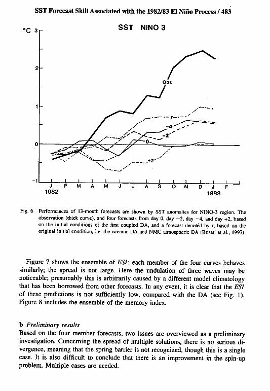
a The case of 1982/83Figure 6 displays five curves of SST anomalies in the NINO-3 region; Fig. 7displays four curves of the ENSO index, ES1; and Fig. 8 shows four curves ofthe memory index. The model's climatology is borrowed from that of Rosati et al.(1996). The five curves (Fig. 6) start to spread in April, and stay separated fromeach other, the spread being almost the same until January 1983. The ensemble ofSST anomalies is considerably lower in amplitude than the observation, the reasonbeing described earlier. It is noted that the forecasts based on the second versionof the coupled DA (not shown here) are substantially and unacceptably lower thanthe group in this figure. The spread (standard deviation) of the ensemble can becalculated, showing that in April, the spread is slightly greater but not substantially

large.


°c SST NINO 3

rs

.~.-.,.-/.r 4"'~ -===

...,'"

,""-""

+2~" .."" ,,"/

-1

1982 1983

Fig.6 Performances of 13-month forecasts are shown by SST anomalies for NINO-3 region. Theobservation (thick curve), and four forecasts from day 0, day -2, day -4, and day +2, basedon the initial conditions of the first coupled DA, and a forecast denoted by r, based on theoriginal initial condition, i.e. the oceanic DA and NMC atmospheric DA (Rosati et al., 1997).

Figure 7 shows the ensemble of ESI; each member of the four curves behavessimilarly; the spread is not large. Here the undulation of three waves may benoticeable; presumably this is arbitrarily caused by a different model climatologythat has been borrowed from other forecasts. In any event, it is clear that the ESIof these predictions is not sufficiently low, compared with the DA (see Fig. 1).Figure 8 includes the ensemble of the memory index.

b Preliminary resultsBased on the four member forecasts, two issues are overviewed as a preliminaryinvestigation. Concerning the spread of multiple solutions, there is no serious di-vergence, meaning that the spring barrier is not recognized, though this is a singlecase. It is also difficult to conclude that there is an improvement in the spin-upproblem. Multiple cases are needed.


ESI.4

0

-1.0

1982 1983Fig. 7 The same as Fig. 6, but for £51.

.MEMORY

0

\\

\-.\

\\

\\

-\.\

\\

\

-.4

1982 1983Fig. 8 The same as Fig. 6, but for the memory index.


6 Conclusions and commentsIn order to investigate and improve the SST forecast skill associated with EINino/La Nina events, a coupled atmospheric-oceanic model DA has been devel-oped. The scheme is of the continuous data injection type, in which the GCMs areused for the first guess and the incremental components of observed data beyondthe first guess are inserted into the models through the 01. In the atmospheric DA,the dynamic balancing is forced continuously for the incremental parts, while inthe oceanic DA, any balancing is not forced (though desirable). These atmosphericand oceanic DAs are applied to the observed data alternately every 6 hours for10 days, and the initial conditions for the coupled system are obtained (the firstcoupled DA).

This set of initial conditions is used for the ensemble forecasts as a sample caseduring the 1982/83 E1 Nino period. There are two objectives. One is to improvethe forecast in the first 3 months, and the other is to investigate whether the "springbarrier" for the equatorial forecasts really exists.

It is tentatively concluded, based on the 4 member forecasts, that the spread ofensemble forecasts for SST is not small for the 13-month forecast range; the spreadbecomes noticeable after 6 months; however, the spread for the ESJ or the memoryindex is not large; the spring barrier is not recognized clearly in this study (seethe comment below); and, the spin-up issue is not conclusive due to the limitednumber of cases. In particular, it is necessary to establish the climatology for thisprediction system. In order to discuss the spin-up issue, more forecast cases areneeded.

With respect to the spring barrier, an hypothesis is postulated. As is known, theSouthern Oscillation has biennial character (see for example, Barnett, 1991), andthe separation between the warm and the cold phases is considered. If a 13-monthforecast range is within the same phase, the "spring barrier" is not a problem, suchas January 1982-January 1983. On the other hand, if the 13-month range crossesfrom one phase to the other, for example, from January 1983-January 1984, the"spring barrier" may have a disturbing effect. This is an assumption. It will beinteresting to apply the ensemble forecasts to other cases.

As has been mentioned with respect to the first coupled DA, the current drawbackis due to the large systematic bias of the particular coupled GCM; the SST issubstantially lower than the observation, and the surface wind is biased in a certainway. In other words, this GCM is not of a great help for DA. The DA scheme shouldbe modified with respect to the model bias utilizing climatological information.

AcknowledgmentThe authors wish to thank William Stem and Richard Gudgel for useful advice.Significant suggestions for improved presentation of the results were offered by TimLi, and useful advice was provided by Yoshio Kurihara and Jerry Mahlman. Specialthanks go to Cathy Raphael, Jeff Varanyak and Wendy Marshall who produced theillustration figures and the manuscript.

486 I K. Miyakoda, J. Ploshay and A. Rosati

ReferencesBALMASEDA. M.A.; M.K. DAVEY and D.L.T. ANDERSON. U. CUBASCH, W.L. GATES, P.R. GENT. M. GHIL. c.

1994. Seasonal dependence of ENSO predic- GORDON, N.C. LAU, C.R. MECHOSO. G.A. MEEHL,tion skill. Climate Research Tech. Note, No. J.M. OBERTUBER, S.G.H. PHILANDER, P.S. SCHOPF,51, Hadley Centre, England, 21 pp. K.R. SPERBER, A. STERL, T. TOKIOKA, J. TRIBBIA

BARNETT. T.P. 1991. The interaction of multiple and S.E. ZEBIAK. 1992. Tropical air-sea interac-time scales in the tropical climate system. J. tion in general circulation models. Clim. Dyn.Clim. 4: 269-285. 7: 75-104.

-; N. GRAHAM, M. CANE, S. ZEBIAK, S. DOLAN. J. PHILANDER. S.G.H. and A.D. SEIGEL. 1985. Simula-O'BRIEN and D. LEGLER. 1988. On prediction of tion of EI Niiio of 1982-83. In: Coupled Ocean-the EI Niiio of 1986-87. Science, 241: 109-196. Atmosphere Models, J.G.J. Nihoul (Ed.), Else-

BLUMENTHAL, M.B. 1991. Predictability of a coupled vier Oceanography Series, No. 40, pp. 517-541.ocean-atmosphere model. J. Clim. 4: 766-784. PLOSHAY, JJ.; W.F. STERN and K. MIYAKODA. 1992.

BRANKOVIC, C.; T.N. PALMER and L. FERRANTI. 1994. FGGE reanalysis at GFDL. Mon. Weather Rev.Predictability of seasonal atmospheric varia- 120: 2083-2108.tions. J. Clim. 7: 217-237. REYNOLDS, R.W. 1988. A real time global sea sur-

CANE, M.A. and S.E. ZEBIAK. 1985. A theory for face temperature analysis. J. Clim. 1: 75-86.EI Niiio and the Southern Oscillation. Science, ROSATI. A.; R.G. GUDGEL and K. MIYAKODA. 1995.228: 1084-1087. Decadal analysis produced from an ocean data

-; -and s.c. DOLAN. 1986. Experi- assimilation system. Mon. W~ather Rev. 123:

mental forecasts of EI Niiio. Science, 321: 827- 2206-2228.832. -; K. MIYAKODA and R.G. GUDGEL. 1997. The

DALEY. R. and K. PURl. 1980. Four-dimensional impact of oceanic initial conditions on ENSOdata assimilation and the slow manifold. Mon. forecasting with a coupled model. Mon. WeatherWeather Rev. 108: 85-99. Rev. 125: 255-273.

DERBER, J. and A. ROSATI. 1989. A global oceanic SAUSEN. R.; K. BARTHELS and K. HASSELMANN. 1988.data assimilation system. J. Phys. Oceanogr. Coupled ocean-atmospheric models with flux19: 1333-1347. correction. Clim Dyn. 2: 154-,163.

GENT. P.R. and JJ. TRIBBIA. 1993. Simulation and SCHNEIDER, E.K.; B. HUANG and J. SHUKLA. 1995.predictability in a coupled TOGA model. J. Ocean wave dynamics and EI Niiio. J. Clim.Clim.6: 1843-1858. 8: 2415-2439.

GOSWAMI. B.N. and J. SHUKLA. 1993. Predictability STERN, W.F. and JJ. PLOSHAY. 1992. A schemeof a coupled ocean-atmospheric flow. J. Atmos. for continuous data assimilation. Mon. WeatherSci. 4: 3-22. Rev. 120: 1417-1432.

LAPRISE. R. 1993. The resolution of global spec- TROUP, AJ. 1965. The Southern oscillation. Q. J. R.lral models. Bull. Am Mereorol. Soc. 73: 1453- Meteorol. Soc. 91: 490-506.1454. TRENBERTH, K.E. 1976. Spatial and temporal varia-

LATIF, M. and N.E. GRAHAM. 1991. How much pre- tions of the Southern Oscillation. Q. J. R. Me-dictive skill is contained in the thermal structure teorol. Soc. 102: 639-653.of an OGCM? TOGA Notes, 2: 6-8. WEBSTER, PJ. and s. YANG. 1992. Monsoon and

LUTHER. D.S.; D.E. HARRISON and R.A. KNOX. 1983. ENSO. Selectively interactive systems. Q. J. R.Zonal winds in the central equatorial Pacific and Meteorol. Soc. 118: 877-926.EI Niiio. Science, 222: 327-330. WERGEN. w. 1987. Diabatic non-linear normal mode,

MIYAKODA. K.; A. ROSATI and R. GUDGEL. 1993. To- initialization for a spectral model with a hybridward the GCM EI Niiio simulation. In: Pre- vertical coordinate. ECMWF Tech. Rept., 59;diction of Interannual Climate Variations, J. available from ECMWF, Reading, UK, 83 pp.Shukla (Ed.), NATO ASI Series, 16, Springer- ZEBIAK, S.E. and M.A. CANE. 1987. A model El Niiio-Verlag, Berlin and Heidelberg, pp. 125-151. Southern Oscillation. Mon. Weather Rev. 115:

NEELlN, J.D.; M. LATIF. M.A.F. ALLAART, M.A. CANE, 2262-2278.

Documents

PRELIMINARY STUDY ON SST FORECAST SKILL … · RESUME Une nude anterieure de Rosati et al. (IY55) a opine que la previ.\ion du El Nino