Embed Size (px)
Citation preview
IFASD-2011-108
PRELIMINARY COMPUTATIONAL ANALYSIS OF THEHIRENASD CONFIGURATION IN PREPARATION FOR
THE AEROELASTIC PREDICTION WORKSHOP
Pawel Chwalowski, Jennifer P. Florance, Jennifer Heeg, Carol D. Wieseman,Boyd Perry, III1
1Aeroelasticity BranchNASA Langley Research Center
Hampton, VA 23681USA
[email protected], [email protected],[email protected], [email protected],
Keywords: Computational Aeroelasticity, Unsteady Aerodynamics, Static Aeroelastic,Dynamic Aeroelastic, Aeroelastic Prediction Workshop, HIRENASD, AGARD 445.6.
Abstract: This paper presents preliminary computational aeroelastic analysis resultsgenerated in preparation for the first Aeroelastic Prediction Workshop (AePW). Theseresults were produced using FUN3D software developed at NASA Langley and are com-pared against the experimental data generated during the HIgh REynolds Number Aero-Structural Dynamics (HIRENASD) Project. The HIRENASD wind-tunnel model wastested in the European Transonic Windtunnel in 2006 by Aachen University′s Departmentof Mechanics with funding from the German Research Foundation. The computationaleffort discussed here was performed (1) to obtain a preliminary assessment of the ability ofthe FUN3D code to accurately compute physical quantities experimentally measured onthe HIRENASD model and (2) to translate the lessons learned from the FUN3D analysisof HIRENASD into a set of initial guidelines for the first AePW, which includes test casesfor the HIRENASD model. This paper compares the computational and experimentalresults obtained at Mach 0.8 for a Reynolds number of 7 million based on chord, corre-sponding to the HIRENASD test conditions No. 132 and No. 159. Aerodynamic loadsand static aeroelastic displacements are compared at two levels of the grid resolution.Harmonic perturbation numerical results are compared with the experimental data usingthe magnitude and phase relationship between pressure coefficients and displacement. Adynamic aeroelastic numerical calculation is presented at one wind-tunnel condition in theform of the time history of the generalized displacements. Additional FUN3D validationresults are also presented for the AGARD 445.6 wing data set. This wing was tested inthe Transonic Dynamics Tunnel and is commonly used in the preliminary benchmarkingof computational aeroelastic software.
1 INTRODUCTION
The fundamental technical challenge in computational aeroelasticity is the accurate pre-diction of unsteady aerodynamic phenomena and their effect on the aeroelastic responseof a vehicle. Currently, a benchmarking “standard” for use in validating the accuracy ofcomputational aeroelasticity codes does not exist. Many aeroelastic data sets have beenobtained in wind-tunnel and flight testing; however, none have been globally recognizedas an ideal data set. There are numerous reasons for this. One is that often such aeroe-lastic data sets focus on the aeroelastic phenomena alone (flutter, for example) and do
1
not contain associated information, such as unsteady pressures or structural deflections.Other available data sets focus solely on the unsteady pressures and do not address theaeroelastic phenomena. Other deficiencies can include omission of relevant data, such asflutter frequency, or the acquisition of only qualitative deflection data. In addition to thesecontent deficiencies, all of the available data sets present both experimental and computa-tional technical challenges. Experimental issues include facility influences, nonlinearitiesbeyond those being modeled, and data post processing. From the computational per-spective, technical challenges include modeling geometric complexities, coupling betweenthe flow and the structure, turbulence modeling, grid issues, and boundary conditions.An Aeroelasticity Benchmark Assessment task was initiated at NASA Langley in October2009 with the primary objectives of (1) examining the existing potential experimental datasets and selecting the one(s) viewed as the most suitable for computational benchmarkingand (2) performing an initial computational evaluation of these configurations using theNASA Langley-developed computational aeroelastic (CAE) software FUN3D [1] as partof its code validation process. A successful effort will result in the identification of a focusproblem for government, industry, and academia to use in demonstrating and comparingcodes, methodologies, and experimental data to advance the state of the art. Ideally, sucha focus problem would be but the first of many put forth for this purpose, with a futuregoal being the design, fabrication, and testing of an aeroelastic model recognized by thecommunity as a benchmark aeroelastic standard.
Excellent examples of such a progression and escalation of code validation in the interna-tional community are the series of four AIAA Drag Prediction Workshops (DPWs) [2] thathave been held since 2001 and the AIAA High Lift Prediction Workshop (HiLiftPW) [3]that was held in 2010. These workshops had three main objectives. The first was to assessthe ease and practicality of using state-of-the-art computational methods for aerodynamicload prediction. The second was to impartially evaluate the effectiveness of the Navier-Stokes solvers, and the final objective was to identify areas for improvement. The structureof the DPW and the HiLiftPW provides a template for other computational communitiesseeking similar improvements in accuracy within their own fields. The examination andselection of aeroelastic data sets within the Aeroelasticity Benchmark Assessment tasktogether with the computational evaluation of these configurations led to initiation of anAeroelastic Prediction Workshop (AePW) series [4].
The main focus of this paper will be on comparing the computational aeroelastic resultsgenerated using FUN3D software against the corresponding experimental data acquiredduring the HIgh REynolds Number Aero-Structural Dynamics (HIRENASD) project [5–7], which has also been selected to be part of the first AePW. This computational effortwas performed to obtain a preliminary assessment of the ability of the FUN3D code toaccurately compute quantities experimentally measured on the HIRENASD model andto begin the work of establishing guidelines for the AePW. A secondary intent of thispaper is to show additional validation of FUN3D using the AGARD 445.6 wing data set,focusing on prediction of the flutter boundary.
Information relevant to the numerical methods employed will be presented first, includ-ing those for grid generation and rigid steady, static aeroelastic, forced oscillation, anddynamic aeroelastic analyses. Details associated with the AGARD 445.6 wing and HIRE-NASD analyses will then be presented.
2
2 NUMERICAL METHOD
2.1 Grid Generation
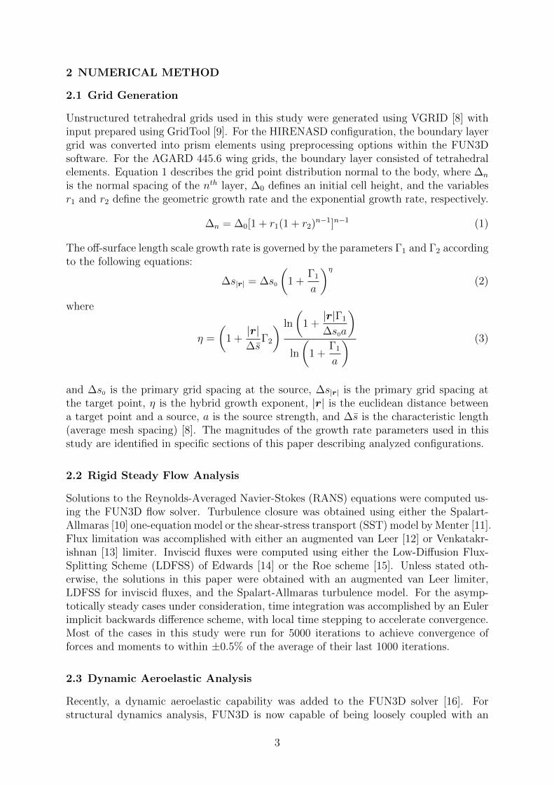
Unstructured tetrahedral grids used in this study were generated using VGRID [8] withinput prepared using GridTool [9]. For the HIRENASD configuration, the boundary layergrid was converted into prism elements using preprocessing options within the FUN3Dsoftware. For the AGARD 445.6 wing grids, the boundary layer consisted of tetrahedralelements. Equation 1 describes the grid point distribution normal to the body, where ∆n
is the normal spacing of the nth layer, ∆0 defines an initial cell height, and the variablesr1 and r2 define the geometric growth rate and the exponential growth rate, respectively.
∆n = ∆0[1 + r1(1 + r2)n−1]n−1 (1)
The off-surface length scale growth rate is governed by the parameters Γ1 and Γ2 accordingto the following equations:
∆s|r| = ∆s0
(1 +
Γ1
a
)η
(2)
where
η =
(1 +|r|∆s̄
Γ2
) ln
(1 +|r|Γ1
∆s0a
)ln
(1 +
Γ1
a
) (3)
and ∆s0 is the primary grid spacing at the source, ∆s|r| is the primary grid spacing atthe target point, η is the hybrid growth exponent, |r| is the euclidean distance betweena target point and a source, a is the source strength, and ∆s̄ is the characteristic length(average mesh spacing) [8]. The magnitudes of the growth rate parameters used in thisstudy are identified in specific sections of this paper describing analyzed configurations.
2.2 Rigid Steady Flow Analysis
Solutions to the Reynolds-Averaged Navier-Stokes (RANS) equations were computed us-ing the FUN3D flow solver. Turbulence closure was obtained using either the Spalart-Allmaras [10] one-equation model or the shear-stress transport (SST) model by Menter [11].Flux limitation was accomplished with either an augmented van Leer [12] or Venkatakr-ishnan [13] limiter. Inviscid fluxes were computed using either the Low-Diffusion Flux-Splitting Scheme (LDFSS) of Edwards [14] or the Roe scheme [15]. Unless stated oth-erwise, the solutions in this paper were obtained with an augmented van Leer limiter,LDFSS for inviscid fluxes, and the Spalart-Allmaras turbulence model. For the asymp-totically steady cases under consideration, time integration was accomplished by an Eulerimplicit backwards difference scheme, with local time stepping to accelerate convergence.Most of the cases in this study were run for 5000 iterations to achieve convergence offorces and moments to within ±0.5% of the average of their last 1000 iterations.
2.3 Dynamic Aeroelastic Analysis
Recently, a dynamic aeroelastic capability was added to the FUN3D solver [16]. Forstructural dynamics analysis, FUN3D is now capable of being loosely coupled with an
3
external finite element solver [17], or in the case of the linear structural dynamics used inthis study, an internal modal structural solver can be utilized. This modal solver is formu-lated and implemented in FUN3D in a similar manner to other Langley aeroelastic codes(CAP-TSD [18] and CFL3D [19]). For the computations presented here, the structuralmodes were obtained via a normal modes analysis (solution 103) with the Finite ElementModel (FEM) solver MSC NastranTM [20]. Modes were interpolated to the surface meshusing the method developed by Samareh [21].
The dynamic analysis was performed in a three-step process. First, the steady CFD so-lution was obtained on the rigid vehicle. Next, a static aeroelastic solution was obtainedby continuing the CFD analysis in a time accurate mode, allowing the structure to de-form. A high value of structural damping (0.99) was used so the structure could findits equilibrium position with respect to the mean flow before the dynamic response wasstarted. Finally, for the dynamic response, the damping was set to the expected value(0.00), and the structure was perturbed in generalized velocity for each of the modesincluded in the structural model. The flow was then solved in the time accurate mode. Itshould be noted that a user-specified modal motion is available in FUN3D. In this study,for harmonic perturbation, the modal displacement for mode n was computed as:
qn = Ansin(ωnt) (4)
where An is amplitude, ωn is frequency, and t is time.
3 AGARD 445.6 WING ANALYSIS
The AGARD 445.6 wing was tested in the Transonic Dynamics Tunnel (TDT) in 1961 [22].Flutter data from this test has been publicly available for over 20 years and has beenwidely used for preliminary computational aeroelastic benchmarking. The AGARD wingplanform was sidewall-mounted and had a quarter-chord sweep angle of 45 degrees, anaspect ratio of 1.65, a taper ratio of 0.66, a wing semispan of 2.5 feet, a wing root chordof 1.833 feet, and a symmetric airfoil. The wing was flutter tested in both air and R-12heavy gas test mediums at Mach numbers from 0.34 to 1.14 at zero-degrees angle of attack.Unfortunately, this data set lacks unsteady surface pressure measurements necessary formore extensive code validation.
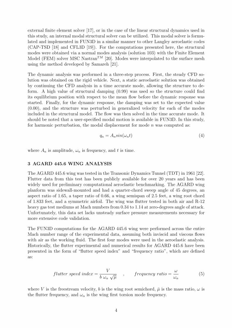
The FUN3D computations for the AGARD 445.6 wing were performed across the entireMach number range of the experimental data, assuming both inviscid and viscous flowswith air as the working fluid. The first four modes were used in the aeroelastic analysis.Historically, the flutter experimental and numerical results for AGARD 445.6 have beenpresented in the form of “flutter speed index” and “frequency ratio”, which are definedas:
flutter speed index =V
b ωα√µ̄
, frequency ratio =ω
ωα(5)
where V is the freestream velocity, b is the wing root semichord, µ̄ is the mass ratio, ω isthe flutter frequency, and ωα is the wing first torsion mode frequency.
4
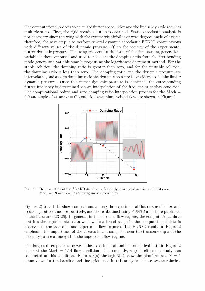
The computational process to calculate flutter speed index and the frequency ratio requiresmultiple steps. First, the rigid steady solution is obtained. Static aeroelastic analysis isnot necessary since the wing with the symmetric airfoil is at zero-degrees angle of attack;therefore, the next step is to perform several dynamic aeroelastic FUN3D computationswith different values of the dynamic pressure (Q) in the vicinity of the experimentalflutter dynamic pressure. The wing response in the form of the time varying generalizedvariable is then computed and used to calculate the damping ratio from the first bendingmode generalized variable time history using the logarithmic decrement method. For thestable solution, the damping ratio is greater than zero, and for the unstable solution,the damping ratio is less than zero. The damping ratio and the dynamic pressure areinterpolated, and at zero damping ratio the dynamic pressure is considered to be the flutterdynamic pressure. Once this flutter dynamic pressure is identified, the correspondingflutter frequency is determined via an interpolation of the frequencies at that condition.The computational points and zero damping ratio interpolation process for the Mach =0.9 and angle of attack α = 0◦ condition assuming inviscid flow are shown in Figure 1.
Figure 1: Determination of the AGARD 445.6 wing flutter dynamic pressure via interpolation atMach = 0.9 and α = 0◦ assuming inviscid flow in air.
Figures 2(a) and (b) show comparisons among the experimental flutter speed index andfrequency ratio values, respectively, and those obtained using FUN3D and those publishedin the literature [23–26]. In general, in the subsonic flow regime, the computational datamatches the experimental data well, while a broad range in the computational data isobserved in the transonic and supersonic flow regimes. The FUN3D results in Figure 2emphasize the importance of the viscous flow assumption near the transonic dip and thenecessity to use a fine grid in the supersonic flow regime.
The largest discrepancies between the experimental and the numerical data in Figure 2occur at the Mach = 1.14 flow condition. Consequently, a grid refinement study wasconducted at this condition. Figures 3(a) through 3(d) show the planform and Y = 1plane views for the baseline and fine grids used in this analysis. These two tetrahedral
5
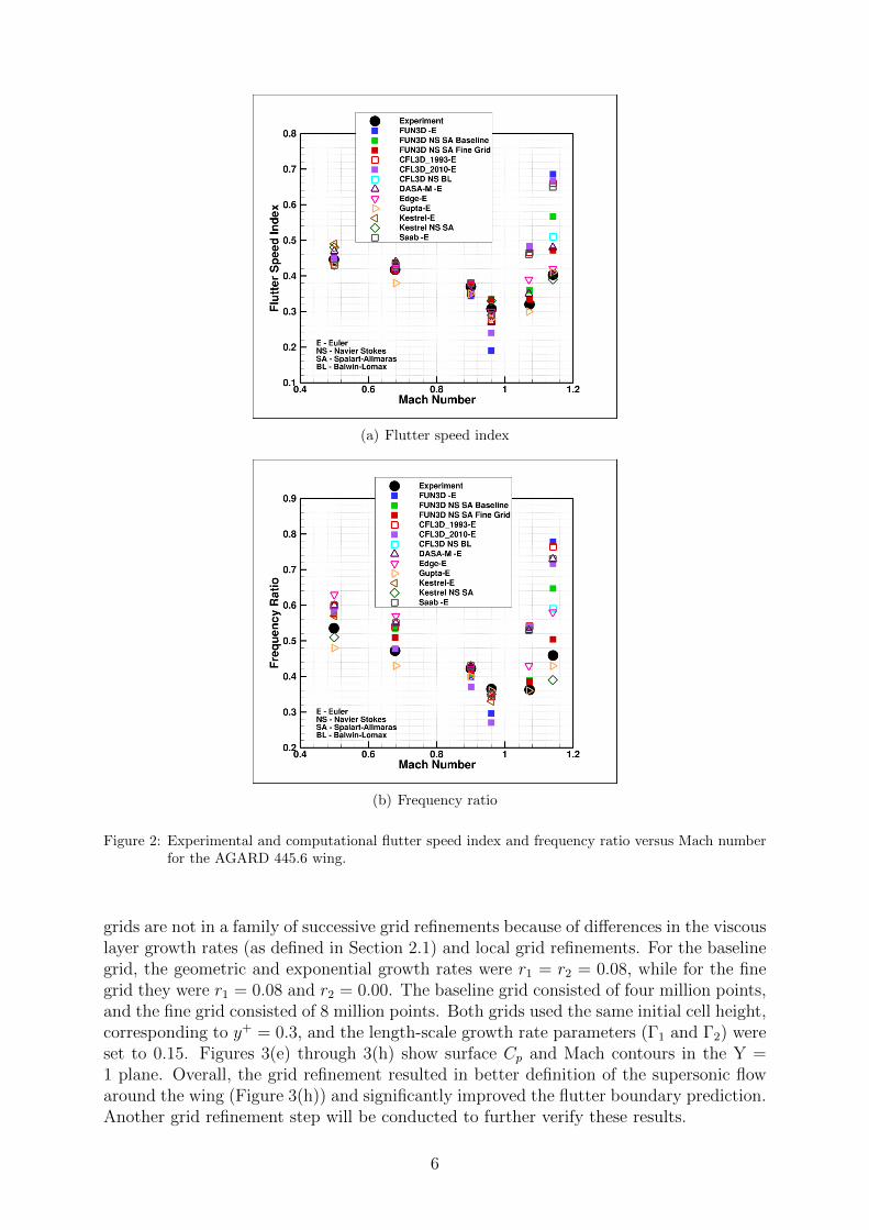
(a) Flutter speed index
(b) Frequency ratio
Figure 2: Experimental and computational flutter speed index and frequency ratio versus Mach numberfor the AGARD 445.6 wing.
grids are not in a family of successive grid refinements because of differences in the viscouslayer growth rates (as defined in Section 2.1) and local grid refinements. For the baselinegrid, the geometric and exponential growth rates were r1 = r2 = 0.08, while for the finegrid they were r1 = 0.08 and r2 = 0.00. The baseline grid consisted of four million points,and the fine grid consisted of 8 million points. Both grids used the same initial cell height,corresponding to y+ = 0.3, and the length-scale growth rate parameters (Γ1 and Γ2) wereset to 0.15. Figures 3(e) through 3(h) show surface Cp and Mach contours in the Y =1 plane. Overall, the grid refinement resulted in better definition of the supersonic flowaround the wing (Figure 3(h)) and significantly improved the flutter boundary prediction.Another grid refinement step will be conducted to further verify these results.
6
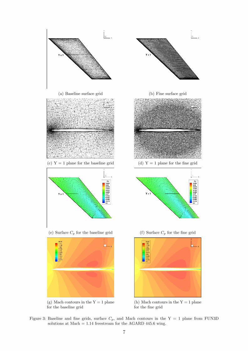
(a) Baseline surface grid (b) Fine surface grid
(c) Y = 1 plane for the baseline grid (d) Y = 1 plane for the fine grid
(e) Surface Cp for the baseline grid (f) Surface Cp for the fine grid
(g) Mach contours in the Y = 1 planefor the baseline grid
(h) Mach contours in the Y = 1 planefor the fine grid
Figure 3: Baseline and fine grids, surface Cp, and Mach contours in the Y = 1 plane from FUN3Dsolutions at Mach = 1.14 freestream for the AGARD 445.6 wing.
7
4 HIGH REYNOLDS NUMBER AERO-STRUCTURAL DYNAMICS(HIRENASD) PROJECT
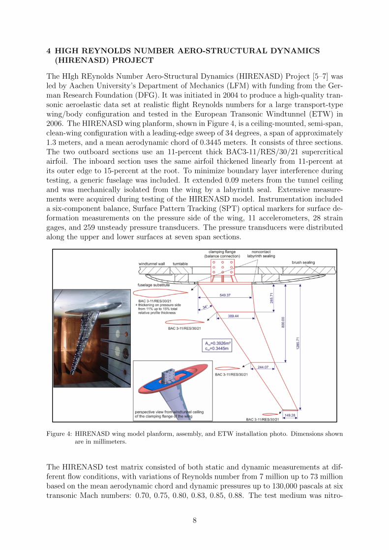
The HIgh REynolds Number Aero-Structural Dynamics (HIRENASD) Project [5–7] wasled by Aachen University’s Department of Mechanics (LFM) with funding from the Ger-man Research Foundation (DFG). It was initiated in 2004 to produce a high-quality tran-sonic aeroelastic data set at realistic flight Reynolds numbers for a large transport-typewing/body configuration and tested in the European Transonic Windtunnel (ETW) in2006. The HIRENASD wing planform, shown in Figure 4, is a ceiling-mounted, semi-span,clean-wing configuration with a leading-edge sweep of 34 degrees, a span of approximately1.3 meters, and a mean aerodynamic chord of 0.3445 meters. It consists of three sections.The two outboard sections use an 11-percent thick BAC3-11/RES/30/21 supercriticalairfoil. The inboard section uses the same airfoil thickened linearly from 11-percent atits outer edge to 15-percent at the root. To minimize boundary layer interference duringtesting, a generic fuselage was included. It extended 0.09 meters from the tunnel ceilingand was mechanically isolated from the wing by a labyrinth seal. Extensive measure-ments were acquired during testing of the HIRENASD model. Instrumentation includeda six-component balance, Surface Pattern Tracking (SPT) optical markers for surface de-formation measurements on the pressure side of the wing, 11 accelerometers, 28 straingages, and 259 unsteady pressure transducers. The pressure transducers were distributedalong the upper and lower surfaces at seven span sections.
Figure 4: HIRENASD wing model planform, assembly, and ETW installation photo. Dimensions shownare in millimeters.
The HIRENASD test matrix consisted of both static and dynamic measurements at dif-ferent flow conditions, with variations of Reynolds number from 7 million up to 73 millionbased on the mean aerodynamic chord and dynamic pressures up to 130,000 pascals at sixtransonic Mach numbers: 0.70, 0.75, 0.80, 0.83, 0.85, 0.88. The test medium was nitro-
8
gen. For static testing, pressure distribution and lift and drag coefficients were acquiredat various angles of attack. Dynamic testing involved forced vibrations of the wing at thenatural frequencies of the first bending, second bending, and first torsion modes and wasperformed over the range of Reynolds numbers at different angles of attack.
The focus of this paper is on comparing the computational results obtained using FUN3Dwith the HIRENASD experimental test cases No. 132 for angle-of-attack sweep andNo. 159, where the model was harmonically excited at the second bending mode fre-quency. The rest of this section is organized in the following way. First, the description ofthe grids used in the analysis is presented. Next, the finite element model and the issuesencountered with interpolating the mode shapes to the surface mesh are described. Therigid steady and the static aeroelastic results are then compared together against the ex-perimental data. Next, the harmonic excitation experimental data are compared againstthe unsteady computational results. Finally, some computational dynamic aeroelasticresults are briefly introduced.
4.1 Unstructured Grids
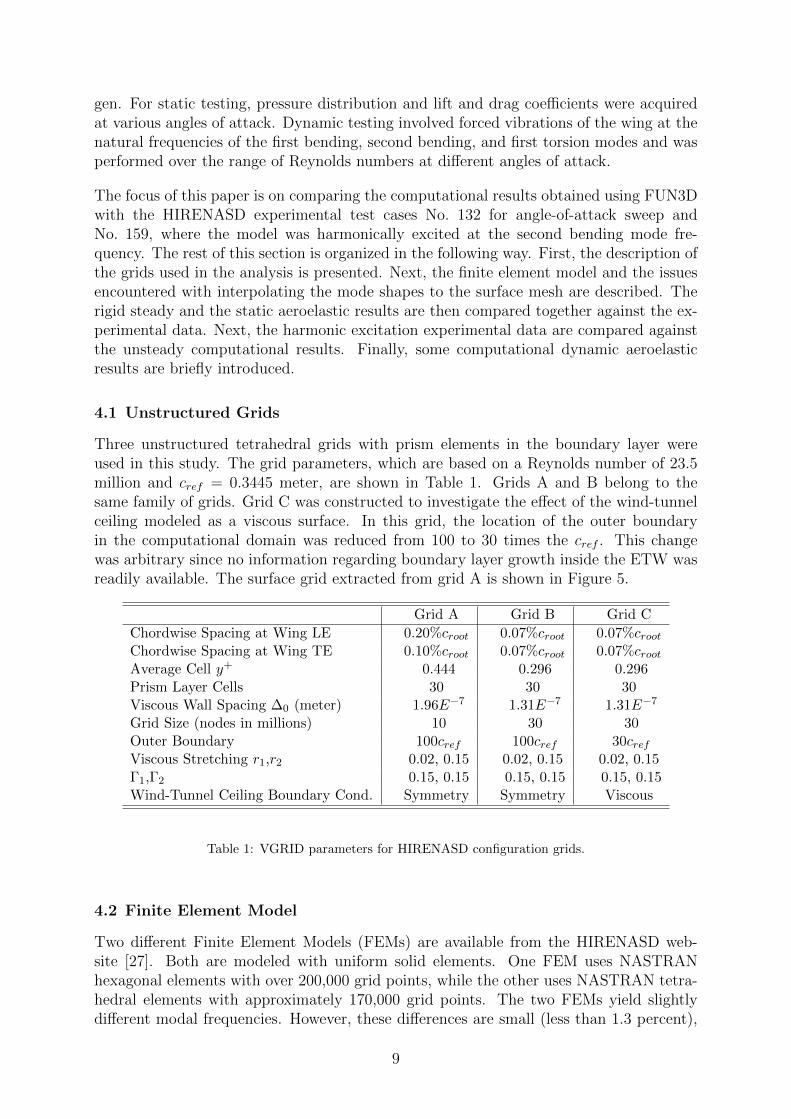
Three unstructured tetrahedral grids with prism elements in the boundary layer wereused in this study. The grid parameters, which are based on a Reynolds number of 23.5million and cref = 0.3445 meter, are shown in Table 1. Grids A and B belong to thesame family of grids. Grid C was constructed to investigate the effect of the wind-tunnelceiling modeled as a viscous surface. In this grid, the location of the outer boundaryin the computational domain was reduced from 100 to 30 times the cref . This changewas arbitrary since no information regarding boundary layer growth inside the ETW wasreadily available. The surface grid extracted from grid A is shown in Figure 5.
Grid A Grid B Grid C
Chordwise Spacing at Wing LE 0.20%croot 0.07%croot 0.07%crootChordwise Spacing at Wing TE 0.10%croot 0.07%croot 0.07%crootAverage Cell y+ 0.444 0.296 0.296Prism Layer Cells 30 30 30Viscous Wall Spacing ∆0 (meter) 1.96E−7 1.31E−7 1.31E−7
Grid Size (nodes in millions) 10 30 30Outer Boundary 100cref 100cref 30crefViscous Stretching r1,r2 0.02, 0.15 0.02, 0.15 0.02, 0.15Γ1,Γ2 0.15, 0.15 0.15, 0.15 0.15, 0.15Wind-Tunnel Ceiling Boundary Cond. Symmetry Symmetry Viscous
Table 1: VGRID parameters for HIRENASD configuration grids.
4.2 Finite Element Model
Two different Finite Element Models (FEMs) are available from the HIRENASD web-site [27]. Both are modeled with uniform solid elements. One FEM uses NASTRANhexagonal elements with over 200,000 grid points, while the other uses NASTRAN tetra-hedral elements with approximately 170,000 grid points. The two FEMs yield slightlydifferent modal frequencies. However, these differences are small (less than 1.3 percent),
9
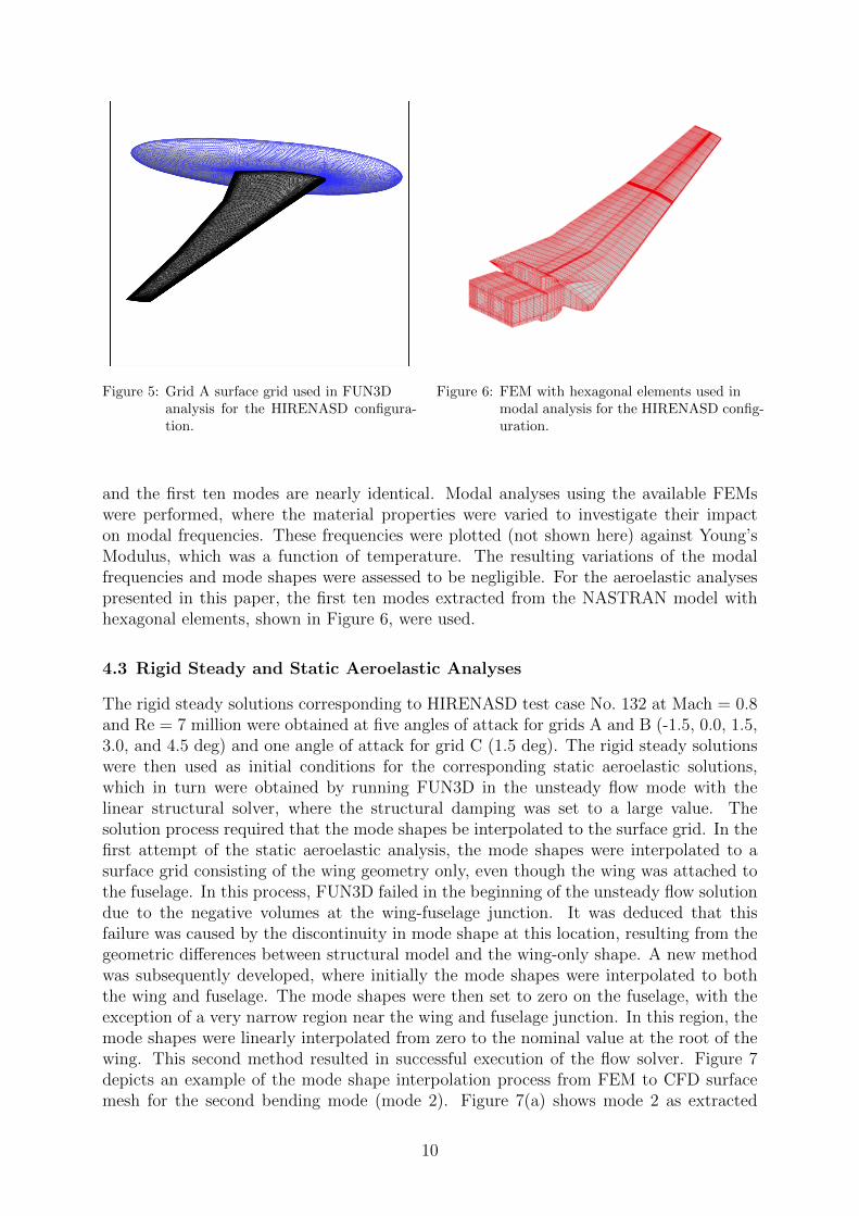
Figure 5: Grid A surface grid used in FUN3Danalysis for the HIRENASD configura-tion.
Figure 6: FEM with hexagonal elements used inmodal analysis for the HIRENASD config-uration.
and the first ten modes are nearly identical. Modal analyses using the available FEMswere performed, where the material properties were varied to investigate their impacton modal frequencies. These frequencies were plotted (not shown here) against Young’sModulus, which was a function of temperature. The resulting variations of the modalfrequencies and mode shapes were assessed to be negligible. For the aeroelastic analysespresented in this paper, the first ten modes extracted from the NASTRAN model withhexagonal elements, shown in Figure 6, were used.
4.3 Rigid Steady and Static Aeroelastic Analyses
The rigid steady solutions corresponding to HIRENASD test case No. 132 at Mach = 0.8and Re = 7 million were obtained at five angles of attack for grids A and B (-1.5, 0.0, 1.5,3.0, and 4.5 deg) and one angle of attack for grid C (1.5 deg). The rigid steady solutionswere then used as initial conditions for the corresponding static aeroelastic solutions,which in turn were obtained by running FUN3D in the unsteady flow mode with thelinear structural solver, where the structural damping was set to a large value. Thesolution process required that the mode shapes be interpolated to the surface grid. In thefirst attempt of the static aeroelastic analysis, the mode shapes were interpolated to asurface grid consisting of the wing geometry only, even though the wing was attached tothe fuselage. In this process, FUN3D failed in the beginning of the unsteady flow solutiondue to the negative volumes at the wing-fuselage junction. It was deduced that thisfailure was caused by the discontinuity in mode shape at this location, resulting from thegeometric differences between structural model and the wing-only shape. A new methodwas subsequently developed, where initially the mode shapes were interpolated to boththe wing and fuselage. The mode shapes were then set to zero on the fuselage, with theexception of a very narrow region near the wing and fuselage junction. In this region, themode shapes were linearly interpolated from zero to the nominal value at the root of thewing. This second method resulted in successful execution of the flow solver. Figure 7depicts an example of the mode shape interpolation process from FEM to CFD surfacemesh for the second bending mode (mode 2). Figure 7(a) shows mode 2 as extracted
10
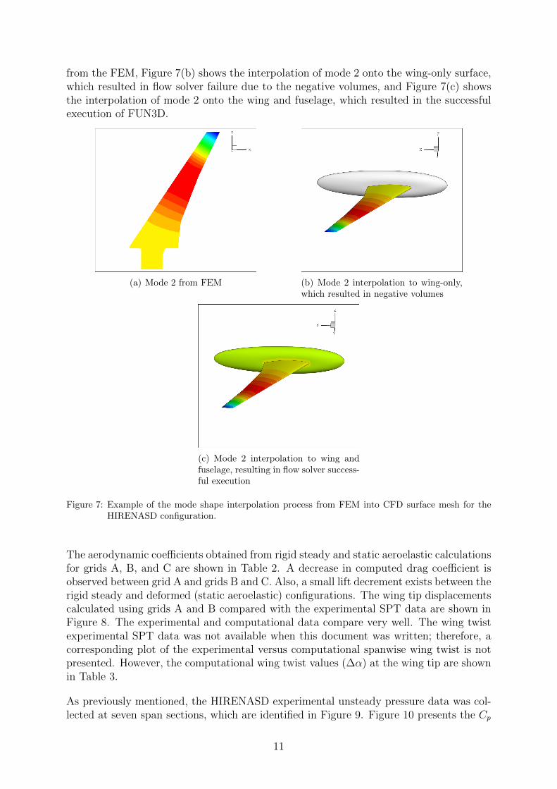
from the FEM, Figure 7(b) shows the interpolation of mode 2 onto the wing-only surface,which resulted in flow solver failure due to the negative volumes, and Figure 7(c) showsthe interpolation of mode 2 onto the wing and fuselage, which resulted in the successfulexecution of FUN3D.
(a) Mode 2 from FEM (b) Mode 2 interpolation to wing-only,which resulted in negative volumes
(c) Mode 2 interpolation to wing andfuselage, resulting in flow solver success-ful execution
Figure 7: Example of the mode shape interpolation process from FEM into CFD surface mesh for theHIRENASD configuration.
The aerodynamic coefficients obtained from rigid steady and static aeroelastic calculationsfor grids A, B, and C are shown in Table 2. A decrease in computed drag coefficient isobserved between grid A and grids B and C. Also, a small lift decrement exists between therigid steady and deformed (static aeroelastic) configurations. The wing tip displacementscalculated using grids A and B compared with the experimental SPT data are shown inFigure 8. The experimental and computational data compare very well. The wing twistexperimental SPT data was not available when this document was written; therefore, acorresponding plot of the experimental versus computational spanwise wing twist is notpresented. However, the computational wing twist values (∆α) at the wing tip are shownin Table 3.
As previously mentioned, the HIRENASD experimental unsteady pressure data was col-lected at seven span sections, which are identified in Figure 9. Figure 10 presents the Cp
11
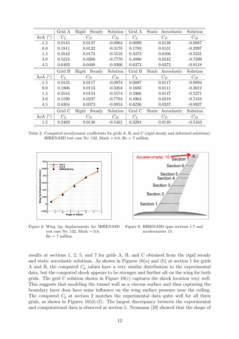
Grid A Rigid Steady Solution Grid A Static Aeroelastic Solution
AoA (◦) CL CD CM CL CD CM-1.5 0.0145 0.0137 -0.0964 0.0099 0.0138 -0.08870.0 0.1811 0.0132 -0.3178 0.1703 0.0131 -0.29971.5 0.3542 0.0173 -0.5516 0.3373 0.0166 -0.52313.0 0.5218 0.0260 -0.7770 0.4996 0.0242 -0.73994.5 0.6493 0.0408 -0.9266 0.6373 0.0372 -0.9118
Grid B Rigid Steady Solution Grid B Static Aeroelastic Solution
AoA (◦) CL CD CM CL CD CM-1.5 0.0135 0.0117 -0.0974 0.0087 0.0117 -0.08940.0 0.1806 0.0113 -0.3204 0.1693 0.0111 -0.30121.5 0.3544 0.0154 -0.5574 0.3366 0.0147 -0.52713.0 0.5190 0.0237 -0.7794 0.4964 0.0219 -0.74164.5 0.6304 0.0373 -0.8954 0.6236 0.0337 -0.8927
Grid C Rigid Steady Solution Grid C Static Aeroelastic Solution
AoA (◦) CL CD CM CL CD CM1.5 0.3469 0.0146 -0.5461 0.3294 0.0140 -0.5163
Table 2: Computed aerodynamic coefficients for grids A, B, and C (rigid steady and deformed solutions):HIRENASD test case No. 132, Mach = 0.8, Re = 7 million.
Figure 8: Wing tip displacements for HIRENASDtest case No. 132, Mach = 0.8,Re = 7 million.
Figure 9: HIRENASD span sections 1-7 andaccelerometer 15.
results at sections 1, 2, 5, and 7 for grids A, B, and C obtained from the rigid steadyand static aeroelastic solutions. As shown in Figures 10(a) and (b) at section 1 for gridsA and B, the computed Cp values have a very similar distribution to the experimentaldata, but the computed shock appears to be stronger and further aft on the wing for bothgrids. The grid C solution shown in Figure 10(c) captures the shock location very well.This suggests that modeling the tunnel wall as a viscous surface and thus capturing theboundary layer does have some influence on the wing surface pressure near the ceiling.The computed Cp at section 2 matches the experimental data quite well for all threegrids, as shown in Figures 10(d)-(f). The largest discrepancy between the experimentaland computational data is observed at section 5. Neumann [28] showed that the shape of
12
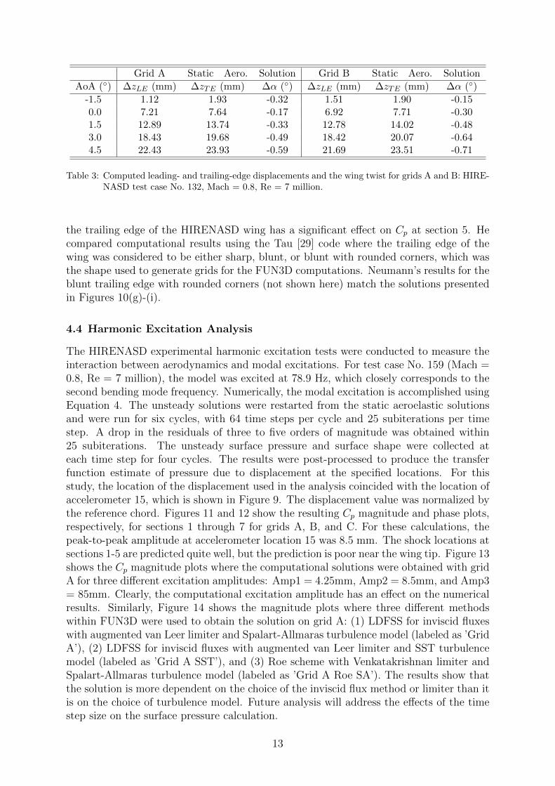
Grid A Static Aero. Solution Grid B Static Aero. Solution
AoA (◦) ∆zLE (mm) ∆zTE (mm) ∆α (◦) ∆zLE (mm) ∆zTE (mm) ∆α (◦)
-1.5 1.12 1.93 -0.32 1.51 1.90 -0.150.0 7.21 7.64 -0.17 6.92 7.71 -0.301.5 12.89 13.74 -0.33 12.78 14.02 -0.483.0 18.43 19.68 -0.49 18.42 20.07 -0.644.5 22.43 23.93 -0.59 21.69 23.51 -0.71
Table 3: Computed leading- and trailing-edge displacements and the wing twist for grids A and B: HIRE-NASD test case No. 132, Mach = 0.8, Re = 7 million.
the trailing edge of the HIRENASD wing has a significant effect on Cp at section 5. Hecompared computational results using the Tau [29] code where the trailing edge of thewing was considered to be either sharp, blunt, or blunt with rounded corners, which wasthe shape used to generate grids for the FUN3D computations. Neumann’s results for theblunt trailing edge with rounded corners (not shown here) match the solutions presentedin Figures 10(g)-(i).
4.4 Harmonic Excitation Analysis
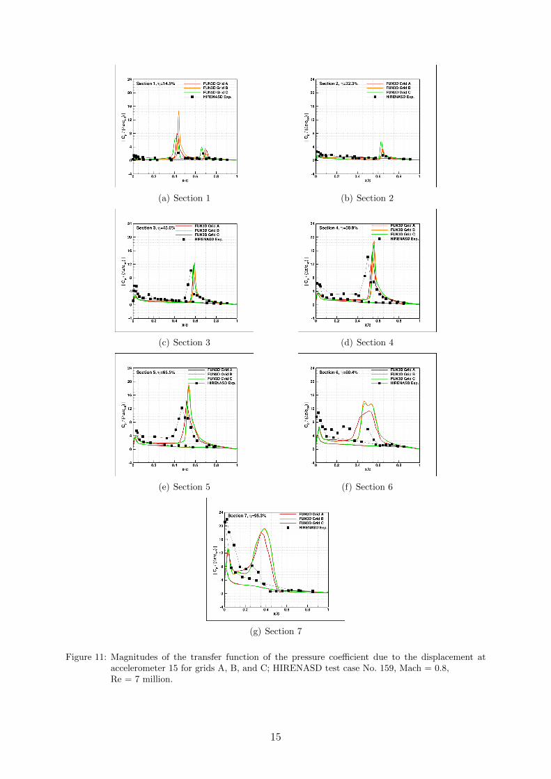
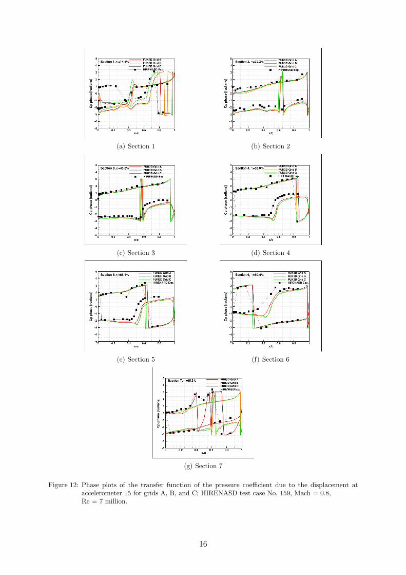
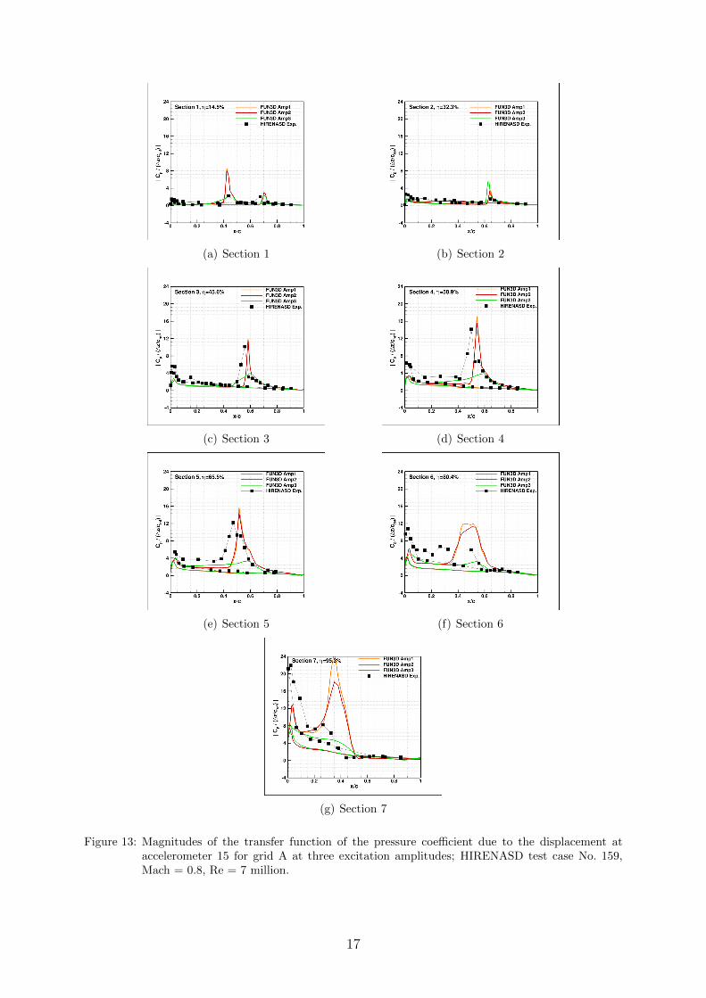
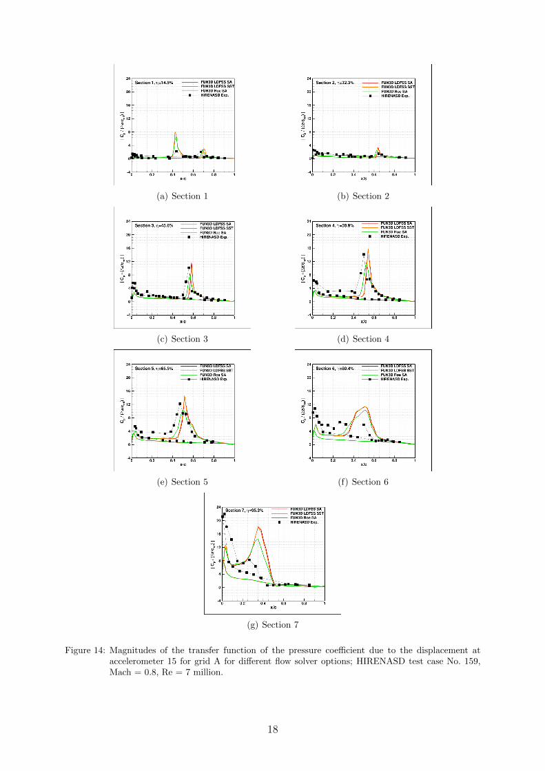
The HIRENASD experimental harmonic excitation tests were conducted to measure theinteraction between aerodynamics and modal excitations. For test case No. 159 (Mach =0.8, Re = 7 million), the model was excited at 78.9 Hz, which closely corresponds to thesecond bending mode frequency. Numerically, the modal excitation is accomplished usingEquation 4. The unsteady solutions were restarted from the static aeroelastic solutionsand were run for six cycles, with 64 time steps per cycle and 25 subiterations per timestep. A drop in the residuals of three to five orders of magnitude was obtained within25 subiterations. The unsteady surface pressure and surface shape were collected ateach time step for four cycles. The results were post-processed to produce the transferfunction estimate of pressure due to displacement at the specified locations. For thisstudy, the location of the displacement used in the analysis coincided with the location ofaccelerometer 15, which is shown in Figure 9. The displacement value was normalized bythe reference chord. Figures 11 and 12 show the resulting Cp magnitude and phase plots,respectively, for sections 1 through 7 for grids A, B, and C. For these calculations, thepeak-to-peak amplitude at accelerometer location 15 was 8.5 mm. The shock locations atsections 1-5 are predicted quite well, but the prediction is poor near the wing tip. Figure 13shows the Cp magnitude plots where the computational solutions were obtained with gridA for three different excitation amplitudes: Amp1 = 4.25mm, Amp2 = 8.5mm, and Amp3= 85mm. Clearly, the computational excitation amplitude has an effect on the numericalresults. Similarly, Figure 14 shows the magnitude plots where three different methodswithin FUN3D were used to obtain the solution on grid A: (1) LDFSS for inviscid fluxeswith augmented van Leer limiter and Spalart-Allmaras turbulence model (labeled as ’GridA’), (2) LDFSS for inviscid fluxes with augmented van Leer limiter and SST turbulencemodel (labeled as ’Grid A SST’), and (3) Roe scheme with Venkatakrishnan limiter andSpalart-Allmaras turbulence model (labeled as ’Grid A Roe SA’). The results show thatthe solution is more dependent on the choice of the inviscid flux method or limiter than itis on the choice of turbulence model. Future analysis will address the effects of the timestep size on the surface pressure calculation.
13
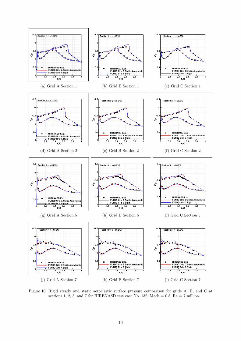
(a) Grid A Section 1 (b) Grid B Section 1 (c) Grid C Section 1
(d) Grid A Section 2 (e) Grid B Section 2 (f) Grid C Section 2
(g) Grid A Section 5 (h) Grid B Section 5 (i) Grid C Section 5
(j) Grid A Section 7 (k) Grid B Section 7 (l) Grid C Section 7
Figure 10: Rigid steady and static aeroelastic surface pressure comparison for grids A, B, and C atsections 1, 2, 5, and 7 for HIRENASD test case No. 132, Mach = 0.8, Re = 7 million.
14
(a) Section 1 (b) Section 2
(c) Section 3 (d) Section 4
(e) Section 5 (f) Section 6
(g) Section 7
Figure 11: Magnitudes of the transfer function of the pressure coefficient due to the displacement ataccelerometer 15 for grids A, B, and C; HIRENASD test case No. 159, Mach = 0.8,Re = 7 million.
15
(a) Section 1 (b) Section 2
(c) Section 3 (d) Section 4
(e) Section 5 (f) Section 6
(g) Section 7
Figure 12: Phase plots of the transfer function of the pressure coefficient due to the displacement ataccelerometer 15 for grids A, B, and C; HIRENASD test case No. 159, Mach = 0.8,Re = 7 million.
16
(a) Section 1 (b) Section 2
(c) Section 3 (d) Section 4
(e) Section 5 (f) Section 6
(g) Section 7
Figure 13: Magnitudes of the transfer function of the pressure coefficient due to the displacement ataccelerometer 15 for grid A at three excitation amplitudes; HIRENASD test case No. 159,Mach = 0.8, Re = 7 million.
17
(a) Section 1 (b) Section 2
(c) Section 3 (d) Section 4
(e) Section 5 (f) Section 6
(g) Section 7
Figure 14: Magnitudes of the transfer function of the pressure coefficient due to the displacement ataccelerometer 15 for grid A for different flow solver options; HIRENASD test case No. 159,Mach = 0.8, Re = 7 million.
18
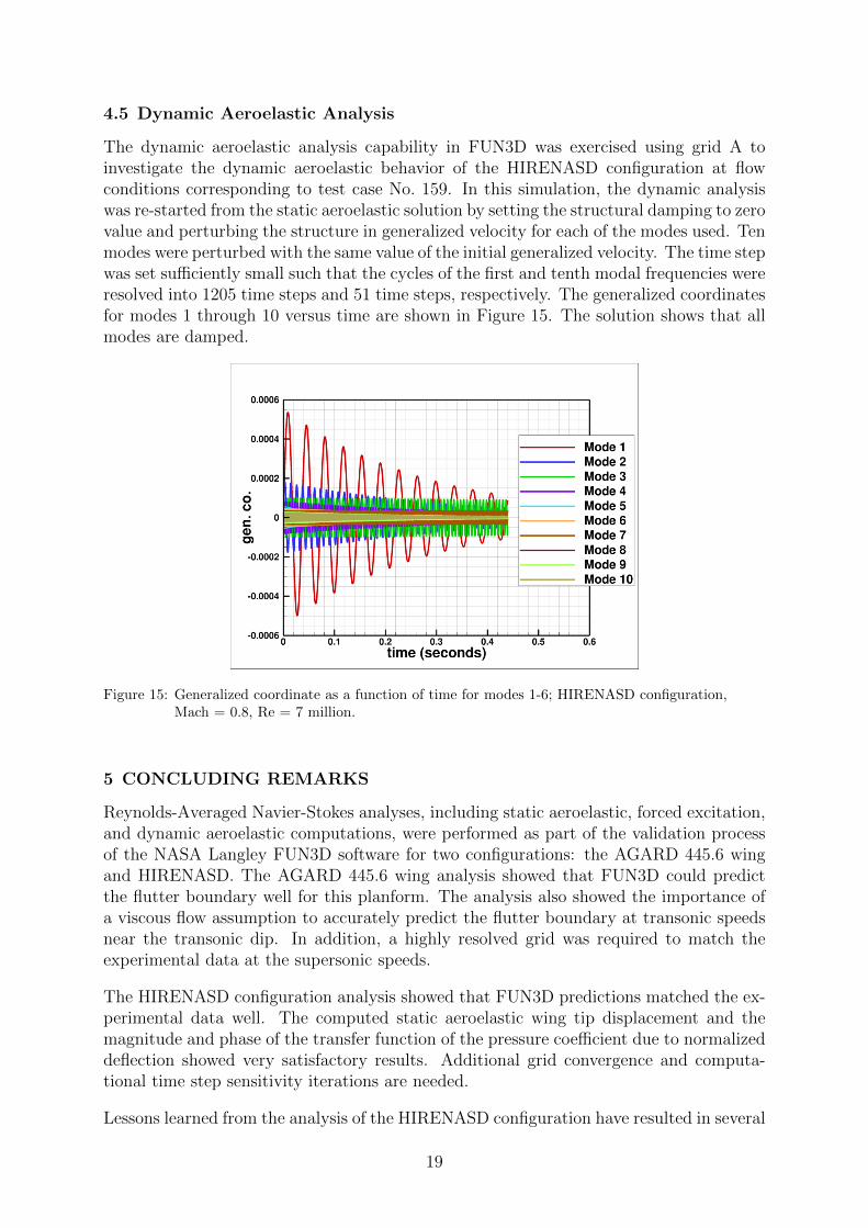
4.5 Dynamic Aeroelastic Analysis
The dynamic aeroelastic analysis capability in FUN3D was exercised using grid A toinvestigate the dynamic aeroelastic behavior of the HIRENASD configuration at flowconditions corresponding to test case No. 159. In this simulation, the dynamic analysiswas re-started from the static aeroelastic solution by setting the structural damping to zerovalue and perturbing the structure in generalized velocity for each of the modes used. Tenmodes were perturbed with the same value of the initial generalized velocity. The time stepwas set sufficiently small such that the cycles of the first and tenth modal frequencies wereresolved into 1205 time steps and 51 time steps, respectively. The generalized coordinatesfor modes 1 through 10 versus time are shown in Figure 15. The solution shows that allmodes are damped.
Figure 15: Generalized coordinate as a function of time for modes 1-6; HIRENASD configuration,Mach = 0.8, Re = 7 million.
5 CONCLUDING REMARKS
Reynolds-Averaged Navier-Stokes analyses, including static aeroelastic, forced excitation,and dynamic aeroelastic computations, were performed as part of the validation processof the NASA Langley FUN3D software for two configurations: the AGARD 445.6 wingand HIRENASD. The AGARD 445.6 wing analysis showed that FUN3D could predictthe flutter boundary well for this planform. The analysis also showed the importance ofa viscous flow assumption to accurately predict the flutter boundary at transonic speedsnear the transonic dip. In addition, a highly resolved grid was required to match theexperimental data at the supersonic speeds.
The HIRENASD configuration analysis showed that FUN3D predictions matched the ex-perimental data well. The computed static aeroelastic wing tip displacement and themagnitude and phase of the transfer function of the pressure coefficient due to normalizeddeflection showed very satisfactory results. Additional grid convergence and computa-tional time step sensitivity iterations are needed.
Lessons learned from the analysis of the HIRENASD configuration have resulted in several
19
recommendations for the first Aeroelastic Prediction Workshop, with the goal of reducinguncertainty across participant-generated results. First, common gridding guidelines thatestablish the definition of a grid family need to be developed. A common finite elementmodel and a common method of interpolating modes to the surface grid must also beestablished. To avoid ambiguities in the surface definition, such as the wing’s trailing-edge geometry, a common baseline geometry is needed. And finally, a common methodfor post-processing the time-accurate data needs to be defined.
6 ACKNOWLEDGMENTS
The authors gratefully acknowledge Dr. Josef Ballmann from Aachen University for mak-ing the HIRENASD data available, discussing the experiment, and agreeing to releasethat data for AePW purposes. The unsteady data were processed with similar methodsshared by Markus Ritter from the German Aerospace Center (DLR). The authors wouldalso like to acknowledge Dr. Jamshid Samareh of NASA Langley for his help in settingup the mode shape interpolation process.
7 REFERENCES
[1] http://fun3d.larc.nasa.gov. NASA Langley Research Center, November 2010.
[2] http://aaac.larc.nasa.gov/tsab/cfdlarc/aiaa-dpw/. August 2010.
[3] http://hiliftpw.larc.nasa.gov/. August 2010.
[4] Heeg, J., Ballmann, J., Bhatia, K., et al. Plans for an Aeroelastic Prediction Work-shop. IFASD Paper 2011-110.
[5] Ballmann, J., Dafnis, A., Korsch, H., et al. Experimental Analysis of High ReynoldsNumber Aero-Structural Dynamics in ETW. AIAA Paper 2008-841.
[6] Ballmann, J., Boucke, A., Dickopp, C., et al. Results of Dynamic Experiments in theHIRENASD Project and Analysis of Observed Unsteady Processes. IFASD Paper2009-103.
[7] Ballmann, J., Dafnis, A., Braun, C., et al. The HIRENASD Project: High ReynoldsNumber Aerostructural Dynamics Experiments in the European Transonic Windtun-nel (ETW). ICAS Paper 2006-726.
[8] Pirzadeh, S. Z. Advanced Unstructured Grid Generation for Complex AerodynamicApplications. AIAA Paper 2008-7178.
[9] Samareh, J. A. Unstructured Grids on NURBS Surfaces. AIAA Paper 1993-3454.
[10] Spalart, P. R. and Allmaras, S. R. A One-Equation Turbulence Model for Aerody-namic Flows. La Recherche Aerospatiale, No. 1, 1994, pp 5–21.
[11] Menter, F. Two-Equation Eddy-Viscosity Turbulence Models for Engineering Appli-cations. AIAA Journal. Vol. 32, No. 8, 1994, pp 1598-1605.
[12] Vatsa, V. N. and White, J. A. Calibration of a Unified Flux Limiter for Ares-ClassLaunch Vehicles from Subsonic to Supersonic Speeds. JANNAF Paper 2009.
20

[13] Venkatakrishnan, V. Convergence to Steady State Solutions of the Euler Equationson Unstructured Grids with Limiter. Journal of Computational Physics. Vol. 118,No. 1, 1995.
[14] Edwards, J. R. A Low-Diffusion Flux-Splitting Scheme for Navier-Stokes Calcula-tions. AIAA Paper 1995–1703.
[15] Roe, P. L. Approximate Riemann Solvers, Parameter Vectors, and DifferenceSchemes. Journal of Computational Physics. Vol. 43, No. 2, 1981.
[16] Biedron, R. T. and Thomas, J. L. Recent Enhancements to the FUN3D Flow Solverfor Moving-Mesh Applications. AIAA Paper 2009-1360.
[17] Biedron, R. T. and Lee-Rausch, E. M. Rotor Airloads Prediction Using UnstructuredMeshes and Loose CFD/CSD Coupling. AIAA Paper 2008-7341.
[18] Batina, J. T., Seidel, D. A., Bland, S. R., et al. Unsteady Transonic Flow Calculationsfor Realistic Aircraft Configurations. AIAA Paper 1987-0850.
[19] Bartels, R. E., Rumsey, C. L., and Biedron, R. T. CFL3D Version 6.4 - GeneralUsage and Aeroelastic Analysis. NASA TM 2006-214301 March 2006.
[20] http://www.mscsoftware.com/. MSC Software, Santa Ana, CA 2008.
[21] Samareh, J. A. Discrete Data Transfer Technique for Fluid-Structure Interaction.AIAA Paper 2007-4309.
[22] Yates, C. E., Land, N. S., and Foughner, J. T. Measured and Calculated Subsonicand Transonic Flutter Characteristics of a 45deg Sweptback Wing Planform in Airand in Freon-12 in the Langley Transonic Dynamics Tunnel. NASA technical NoteD-1616, March 1963.
[23] Lee-Rausch, E. M. and Batina, J. T. Calculation of AGARD Wing 445.6 FlutterUsing Navier-Stokes Aerodynamics. AIAA Paper 1993-3476.
[24] Lee-Rausch, E. M. and Batina, J. T. Wing Flutter Boundary Prediction UsingUnsteady Euler Aerodynamic Method. Journal of Aircraft. Vol. 32, No. 3, 1995.
[25] Gupta, K. K. Development of a Finite Element Aeroelastic Analysis Capability.Journal of Aircraft. Vol. 33, No. 5, 1996.
[26] Pahlavanloo, P. Dynamic Aeroelastic Simulation of the AGARD 445.6 Wing UsingEdge. Technical Report FOI-R-2259-SE, April 2007.
[27] https://heinrich.lufmech.rwth-aachen.de/en/. Aachen University, June 2010.
[28] Neumann, J., Nitzsche, J., and Voss, R. Aeroelastic Analysis by Coupled Non-linearTime Domain Simulation. RTO-MP-AVT-154 2008.
[29] Schwamborn, D., Gerhold, T., and Heinrich, R. The DLR TAU-CODE: RecentApplications in Research and Industry. Tech. rep. Technical Report at EuropeanConference on Computational Fluid Dynamics, ECCOMAS CFD 2006.
21