Preface To Manual For Domenico Non-Steady State Spreadsheet Analytical Model

Preface To Manual For Domenico Non-Steady StateSpreadsheet Analytical Model

Regional Board staff prepared the attached spreadsheet analytical model and model

manual to assist in estimating Methyl Tertiary Butyl Ether (MTBE) and other oxygenates

travel time to a downgradient receptor (usually a domestic supply well). The need for

estimating the plume travel time is part of implementation of the Final Draft Guidelines

for Investigation and Cleanup of MTBE and Other Oxygenates (Final Draft Guidelines)

required by the State Water Resources Control Board. In order to implement the Final

Draft Guidelines, the Los Angeles Regional Board staff have required responsible parties

within the region to develop a site-specific conceptual model, in which the estimate of

plume travel time is required.

The attached model is a Domenico non-steady state analytical model for continuous

source release situation. This model is posted at our website for users’ convenience in

compliance with Regional Board requirements. However, this model is NOT the only

model that can be used to estimate the plume travel time. Other models are also available

for the same purpose and may be utilized. If other models are applied, they will need to

be evaluated on a case by case basis.

If you have any questions about the model, please contact Tom Shih at (213) 576-6729

or Yue Rong at (213) 576-6710.

MANUAL

FOR

DOMENICO NON-STEADY STATE

SPREADSHEET ANALYTICAL MODEL

(FOR CONTINUOUS SOURCE RELEASE)

Tom Shih and Yue Rong

Underground Storage Tank SectionCalifornia Regional Water Quality Control Board - Los Angeles Region

320 West 4th Street, Suite 200, Los Angeles, CA 90013

May 15, 2001

Table of Contents

1. Introduction.……………………………………………………..………………….1

2. Domenico Non-Steady State Spreadsheet Analytical Model…….……..…….……..1

3. Estimation of Centerline Distance………………………………………….……….3

4. Uncertainties Regarding the Time (T0) of Release and Source Concentration (C0).…5

5. Spreadsheet Analytical Model ………………….…………………………………. 6

6. Sensitivity Analysis ………………………………………….……………………. 7

7. Model Input Parameters ……………………………………………………….….. 9

7.1 Dispersivity (αL) ………………………………………….…………….…. 97.2 Groundwater Velocity (v) ………………………………………………....10

8. Case Study ………………………………………….……………………………..11

9. Troubleshooting for the Spreadsheet Analytical Model ………….………..….….. 16

10. Acknowledgments………………………………………………………………...17

11. References………………………………………….…………………………...…17

Figures

Figure 1……………………………………………………………………………………..5

Figure 2……………………………………………………………………………………..7

Figure 3……………………………………………………………………………………19

Manual for Domenico Non-Steady State SpreadsheetAnalytical Model

1

1. Introduction

The Domenico non-steady state analytical model (1987) presented in this manual is ananalytical solution to the advection-dispersion partial-differential equation of organiccontaminant transport processes in groundwater for a continuous release source as describedbelow. The model contains one dimensional groundwater velocity, longitudinal, transverse,and vertical dispersion, the first order degradation rate constant, finite contaminant sourcedimensions, and can estimate travel time to a receptor at contaminant plume centerline, givena continuous release source. Since the plume concentration is a function of travel time in themodel, the analytical model can be applied to estimate the plume travel time to a givendistance for dissolved organic contaminants in groundwater. The use of the analytical modelrequires contaminant temporal concentration data at a minimum of one source and onedowngradient monitoring well. The groundwater temporal concentration data for thedowngradient monitoring well must show a reasonable pattern, in which contaminantconcentrations over time resemble a sigmoidal curve. The model is calibrated by adjustingfour model-input parameters to fit the pattern of groundwater temporal concentrationdistribution at the downgradient monitoring well. The model after calibration is then used toestimate the plume travel time to a given distance (e.g., to a drinking water well). Theanalytical solution form is programmed into a Microsoft Excel Spreadsheet. Prior toapplying the spreadsheet model and interpreting the model results, understanding of modelassumptions and uncertainties associated with model calibration with field data is stronglyadvised.

2. Domenico Non-Steady State Analytical Model

The Domenico non-steady state analytical model is based on the advection-dispersionpartial-differential equation for organic contaminant transport processes in groundwateras described below (Domenico and Robbins, 1985):

(1)

Where C is the contaminant concentration in groundwater (mg/L); t is the time (day); v isthe groundwater seepage velocity (ft/day); x, y, z are the coordinates to the threedimensions (ft); Dx, Dy, Dz are the dispersion coefficients for the x, y, z dimensions(ft2/day), respectively.

x

Cv

z

CD

y

CD

x

CD

t

Czyx ∂

∂−

∂∂

+∂∂

+∂∂

=∂∂

2

2

2

2

2

2


2

In an attempt to incorporate natural degradation factor, Domenico (1987) introduced afirst order degradation rate constant to approximate the original analytical solution toequation (1). To evaluate transient plume behavior, the transient, centerline analyticalsolution derived by Domenico (1987) is applied. Under conditions of a continuoussource and finite source dimensions with one-dimensional groundwater velocity,longitudinal, transverse, and vertical dispersion, and a first order degradation rateconstant, equation (2) shown below represents the Domenico transient solution for thecenterline concentration as a function of time (Domenico, 1987):

(2)

Where C(x,0,0,t) is the contaminant concentration (µg/L) in a downgradient well at time talong the plume centerline at a distance x (x,0,0); C0 is the steady state contaminantconcentration in the source well; x is the centerline distance between the downgradientwell and source well (ft); αx, αy, and αz are the longitudinal, transverse, and verticaldispersivity (ft), respectively; λ is the degradation rate constant (1/day) and equals to0.693/t1/2 (where t1/2 is the degradation half-life of the contaminant); v is the groundwatervelocity (ft/day); Y is the source width (ft); Z is the source depth (ft); erf and erfc are theerror and complementary error functions, respectively; and exp is the exponentialfunction.

The Domenico non-steady state analytical equation (2) assumes:

a. Transient or non steady state (concentration is a function of time),b. A continuous release source,c. Homogeneous aquifer properties,d. One dimensional groundwater flow,e. No change in groundwater flow direction and velocity,f. First order degradation rate,g. Contaminant concentration estimated at the centerline of the plume,

( )( )

+−

×

+−=

2

1

2

1

2

1

0

2

41

411

2exp

2,0,0,

vt

vvtx

erfcv

xCtxC

x

x

x

x α

λαλα

α

( ) ( )

×

×

2

1

2

1

44 x

Zerf

x

Yerf

zy αα


3

h. Molecular diffusion based on concentration gradient is neglected, andi. Adsorption in transport process is neglected.

Key Limitations:

a. The model should not be applied where vertical flow gradients affectcontaminant transport.

b. The model should not be applied where hydrogeologic conditions changedramatically over the simulation domain.

Understanding model assumptions and limitations is crucial to simulate transport processfor a specific contaminant in groundwater. For example, methyl tertiary butyl ether(MTBE) has a very low potential of being sorbed onto soil particles due to its low Koc

value and high solubility in water and therefore adsorption in transport process may beneglected. Conversely, perchloroethylene (PCE) has a relatively high retardationpotential and the model described in this manual need to be modified before it can beapplied for estimating PCE transport process in groundwater. In addition, whencompared to other petroleum hydrocarbons (e.g., benzene, toluene, ethylbenzene, andtotal xylenes [BTEX]), MTBE does not naturally degrade to a significant degree.

3. Estimation of Centerline Distance

One of the conditions for using the Domenico Non-Steady State Analytical Model is thatthe selected downgradient monitoring well must be along the plume centerline. In mostcontamination cases, downgradient monitoring wells may be off the centerline. In orderto apply the Domenico Analytic Model to these cases, the distance between these off-centerline wells and source wells must be converted to the centerline distance.

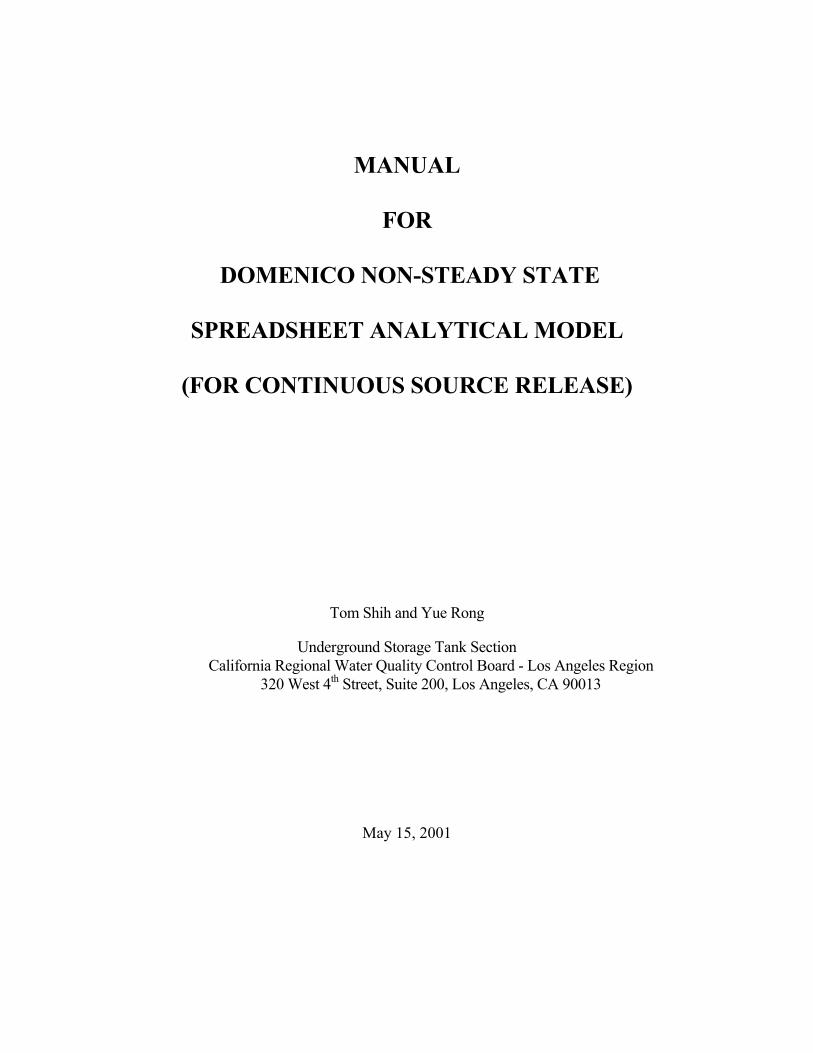
In this manual, an ellipse trigonometry method is used to convert an off-centerlinedistance to a centerline distance (Tong and Rong, 2001). The method is based on anassumption about the contaminant plume geometry, which can be described as an ellipseshape (Figure 1). This ellipse shape is idealized and assumed based on the observationsthat the plume migrates fastest along groundwater flow direction and the longitudinaldispersivity is greater than transverse dispersivity in general. This assumption isconsistent with the shape in a similar study by Martin-Hayden and Robbins (1997).

Based on the assumption of the ellipse plume shape, the following offers the calculationof converting a distance from an off-centerline well to a centerline well. Theassumptions are: (1) the ellipse width = 0.33 ellipse length (most studies assume αy =


4

0.33αx) (the ellipse length/width ratio can be adjusted based on the field data collectedfrom every individual site) and (2) the ellipse is the contaminant iso-concentration line.The equation for an ellipse with a horizontal major axis:

(3)

Where, a = the length of the major axis, b = the length of the minor axis, a > b > 0. X andY are the coordinates to the x and y dimension, respectively. If the source well isassumed at close to one end of the ellipse and one downgradient well located on theellipse (see Figure 1) with an off-centerline distance L', the centerline distance can becalculated as follows.

Since b = 0.33 × a, x1 = Cos θ × L' – a, y1 = Sin θ × L', where θ = the angle between off-centerline and centerline (θ < 90°) and 2a = the distance (x) between source well andprojected downgradient centerline well.

Therefore,

(θ < 90°)

(4)

12

2

2

2

=+b

Y

a

X

( ) ( )( )

133.0

''2

2

2

2

=××

+−×

a

LSin

a

aLCos θθ

( ) 222 )'(18.9' aLSinaLCos =××+−× θθ

( ) '2)'(18.9' 22 LCosaLSinLCos ×××=××+× θθθ

)18.9(''18.9'

222

θθθθ

θθSintgCosL

Cos

LSinLCosaX ××+=

××+×==


5

Y

Figure 1. Plane view of regular plume geometry and groundwater monitoring system(Tong & Rong, 2001)

4. Uncertainties Regarding Initial Time (T0) of Release and SourceConcentration (C0)

As in most contamination cases, the initial time of release (T0) and the mass dischargedare usually unknown. It is thus difficult to determine the exact source concentration (C0).Since one of the assumptions in this analytical model is a continuous source, so ideallythe temporal concentration profile at the source well should be constant over time.However, this is rarely the case. Due to a variety of factors such as changinggroundwater levels, inherent variability of environmental quantification, instrumentationinexactness, sampling error, heterogeneous and varying subsurface environmentalconditions, etc., the contaminant concentration at the source well will not show a constantover time. In order to select one contaminant concentration that best represents thesource concentration over the period of time, an intuitive solution is to select an average(i.e., the mean) or median concentration.

The uncertainties associated with T0 would affect the calibration of model-inputparameters for predicting plume travel time. As the model parameter sensitivity analysisindicates in the later section, the analytical model is sensitive to changes made to T0 (seeTable I). Furthermore, changes made to T0 as well as groundwater velocity (v) would shifthorizontally the time (x-axis) versus normalized concentration (C/C0) plot (y-axis) for themodel predicted and field measured curves relative to each other. The collective impacts

a

b

θ

L'

SourceWell

Off-centerlineWell (x1, y1)

Centerline Down-gradient Well

X0

Groundwater Flow Direction

Iso-concentration line


6

from T0 and v would thus generate large uncertainties in the calibration of model-inputparameters and the prediction of the plume travel time. This problem may be dealt with intwo ways during the model calibration: (1) to obtain relatively accurate site-specificinformation regarding the initial time of release (e.g., time of underground tank leaking, orhistory of contaminant usage), or (2) to use a more conservative value of groundwaterseepage velocity (faster), estimated by the range of groundwater velocities typicallyassociated with certain soil types, formations, and hydrology. Since relatively accurate site-specific information regarding the time of release is generally unavailable or unknown, thelatter approach is more useful and thus is the one applied in this model.

5. Spreadsheet Analytical Model

The analytical model can be applied to estimate the travel time to a receptor for contaminantsin groundwater. Figure 1 shows the model setting. Figure 2 presents a flowchart of theanalytical model application. The downgradient well used to calibrate the model must bedowngradient of the source well and has the maximum concentration less than sourceconcentration C0. Step one, groundwater monitoring data provide temporal concentrationsat one source and one downgradient well with known C(Ti), Ti, and X1 (i = 1,…,n) whereC(Ti) = concentration at downgradient well at time Ti, X1 = downgradient well distance fromthe source well (Figure 1). As was discussed in Section 4, the source concentration C0 maybe selected as the mean or median concentration of the temporal concentration profile. T0

is the initial time of contaminant release. T1 is the time for the first monitoring data pointused to calibrate the model. The groundwater monitoring is conducted periodically. SinceT0 is usually unknown in most cases, T1 or time of the first monitoring data point relative toT0 will also be unknown. However, time T2,…,Tn relative to T1 is known. Thus an educatedjudgement for T1 must be made first, and T2,…,Tn are directly related to T1. Step two, theellipse trigonometry method presented in Section 3 is used to convert off-centerline distanceto centerline distance for the downgradient well location. Step three, the field data areplotted (Ti vs. C(Ti)/C0, i = 1,…,n for the downgradient well). The field data must show atemporal pattern of a “sigmoidal” shape. Step four, the known C(Ti) and Ti, and selectedsource concentration C0 are used to choose values for model parameters αx, v, λ, and T1, bytrial-and-error to fit the data points on the plot generated in step three. Step five, thecalibrated values of the parameters αx, v, λ, and T1 are to be used to predict the travel time toa receptor at a downgradient distance X.

The Domenico Non-Steady State Analytical Model solution form has been programmed intoa user-friendly spreadsheet in Microsoft Excel (version 7.0). The groundwater monitoringdata from a specific site provide C(Ti) and Ti (i = 1,…,n) which are plotted (C(Ti)/C0 vs. Ti).By trial and error method, the model parameters αx, v, λ, and T1 are altered within thereasonable ranges until a best-fit curve to the temporal concentration distribution field data isvisually identified (see example in Section 8). For example, changes made to T1 and


7

groundwater velocity (v) would shift horizontally the time (x-axis) versus normalizedconcentration (C/C0) plot for the model predicted and field measured curves relative toeach other; changes made to αx would primarily affect the spreading of the curve; andchanges made to λ would primarily affect the height of the curve. After a “best-fit” curve isestablished, the calibrated values of αx, v, λ, and T1 are used to predict the travel time t at adowngradient distance X. An example of Excel spreadsheet is demonstrated in Tables V andVI, Section 8.

Figure 2. Domenico Non-Steady State Spreadsheet Analytical Model Flowchart

6. Sensitivity Analysis

A sensitivity analysis as presented in Table I is conducted for the Domenico Non-SteadyState Analytical Model in the same way as presented in Rong et al. (1998). Model runsunder the condition of varying input parameter values, one at a time, within reasonableranges. Then model outputs from various input values are compared with the respective“baseline” cases. The sensitivity analysis results indicate that model output t (time for plume

(1) Collect Field Data: X1,C(Ti), Ti

(i = 1,…,n)

(3) Plot the field data (Ti vs. C(Ti)/C0)(i = 1,…,n)

(4) Calibrate model parameters αx, v, λ, T1, andfind the model best fit curve to the field data

(2) Convert off-centerline distance to centerlinedistance for downgradient well location

(5) Predict the plume travel time at a givendistance away using calibrated model parameters

αx, v, λ, and T1


8

to reach 5 µg/L in downgradient receptor) is relatively sensitive to model input parametersαx, v, and X. The concentration 5 µg/L is used here since it’s the secondary maximumcontaminant level for MTBE. Model output t is not as sensitive to model input parametersY, Z, or λ. However, since model output C(Ti) is sensitive to λ, λ is included along with αx,v, and X to calibrate the model by changing the values of these parameters to fit in the fielddata.

Table I. Sensitivity Analysis Results for Domenico Analytical Model

Input Parameter Factor of Input Changefrom Baseline

Model Output t(years)

Factor of t Differencefrom Baseline

RelativeSensitivity S *

αx (ft) 0.091 (baseline) --- 3.1 ---

0.1 0.1 3.7 1.164 4 2.6 0.84

v (ft/day) 0.190.1 (baseline) --- 3.1 ---

0.25 2.5 1.3 0.420.5 5.0 0.7 0.23

X (ft) 1.23150 (baseline) --- 3.1 ---

100 0.67 1.9 0.61300 2.0 7 2.26

Y (ft) 0.0320 (baseline) --- 3.1 ---

10 0.5 3.2 1.0330 1.5 3.1 1.0

Z (ft) 0.0365 (baseline) --- 3.1 ---

1 0.2 3.3 1.0610 2 3.1 1

λ (1/day) 0.0320.0005 (baseline) --- 3.1 ---

0.001 2 3.2 1.030.002 4 3.4 1.10

* Note (Table 1): Relative sensitivity (S) is calculated using the following equation:

Where x and f are baseline input and model output values, dx and df are input and model output range,respectively.

=

dx

x

f

dfS


9

7. Model Input Parameters

7.1. Dispersivity (αx)

One of the primary parameters that control the fate and transport of contaminant isdispersivity of the aquifer. The Domenico non-steady state analytical model uses thelongitudinal (αx), transverse (αy), and vertical (αz) dispersivities to describe the mechanicalspreading and mixing caused by dispersion. The spreading of a contaminant caused bymolecular diffusion is assumed to be small relative to mechanical dispersion in groundwatermovement and is ignored in the model. Various dispersivity values have been reported instudies. Most of existing studies traditionally use αy and αz as a fraction of αx. For thisrelationship, we only calibrate αx, which relates αy and αz. Table II is a summary of thethree dimensional dispersivity values in literatures.

Table II. Dispersivity Values In Literature

Dispersivity Valves Reference

αx = 0.1 X αy = 0.33 αx

αz = 0.056 αx

Gelhar and Axness (1981)

αx = 0.1 X αy = 0.1 αx

αz = 0.025 αx

Gelhar et al. (1992)

αx = 14 – 323 (ft) αy = 0.13 αx

αz = 0.006 αx

USEPA (1996)

αx = 16.4 (ft) αy = 0.1 αx

αz = 0.002 αx

Martin-Hayden and Robbins (1997)

αx = 0.33 – 328 (ft) αy = 0.1 αx

αz = 0.1 αx

AT123D (1998)

X = the distance to the downgradient well (ft), αx = the longitudinal dispersivity (ft), αy = the transverse dispersivity (ft), αz = the vertical dispersivity (ft).

7.2. Groundwater Velocity (v)

Groundwater velocity in the geologic material is controlled by hydraulic conductivity,hydraulic gradient in the vicinity of the study area, and effective porosity of the geologic


10

material. Based on the Darcy’s Law, the average groundwater velocity can be calculatedusing the following equation:

endx

dhKv

1××= (5)

Where,

v - Groundwater velocity (ft/day)K - Hydraulic conductivity (ft/day)dh/dx - Hydraulic gradient (ft/ft)ne - Effective porosity (dimensionless)

The groundwater hydraulic gradient can be determined from field data. The hydraulicconductivity and effective porosity are also preferably obtained from site-specific testing.The hydraulic conductivity and effective porosity are mainly affected by the geologicmaterial grain size. In cases where site-specific data are absent (i.e., pumping test or slugtest), to estimate groundwater velocity, the lithologic boring logs can be reviewed to identifythe predominant aquifer materials needed to estimate hydraulic conductivity and effectiveporosity to be consistent with value ranges from published references (see Tables III and IV).

Table III. Hydraulic Conductivity Range for Various Classes of Geologic Materials

Hydraulic Conductivity, ft/dayMaterial Todd

1980Bower1978

Freeze & Cherry1979

Dawson & Istok1991

Gravel 5 x 102 – 1 x 103 3 x 102 – 3 x 103 3 x 102 – 3 x 105

Coarse Sand 1 x 102 7 x 101 – 3 x 102

3 x 103 – 3 x 105

Medium Sand 4 x 101 2 x 101 – 7 x 101 3 – 3 x 103

Fine Sand 101 3 - 2 x 101

3 x 10-2 – 3 x 103

3 x 10-2 – 3Silt and Clay 10-3 – 3 x 10-1 3 x 10-8 – 3 x 10-2 3 x 10-7 – 3 x 10-3 3 x 10-6 – 3 x 10-1


11

Table IV. Total Porosities and Effective Porosities of Well-sorted, UnconsolidatedFormations

Material Diameter (mm) Total Porosity (%) Effective Porosity (%)Gravel

Coarse 64.0 – 16.0 28 23Medium 16.0 – 8.0 32 24

Fine 8.0 – 2.0 34 25Sand

Coarse 2.5 – 0.5 39 27Medium 0.5 – 0.25 39 28

Fine 0.25 – 0.162 43 23Silt 0.162 – 0.004 46 8Clay <0.004 42 3SOURCE: Roscoe Moss Company, 1990

8. Case Study

A case study example is included in this manual to demonstrate the modeling procedures forestimating MTBE plume travel time. The case study is a real case from an undergroundstorage tank (UST) release site in the City of Los Angeles, California. Figure 3 depicts thesite layout (USTs, dispenser islands, buildings, and well locations) and site groundwatercontour map with gradient and approximate direction of groundwater flow. The modelingprocedures are described in detail as the following steps:

Step 1:

Find the groundwater contour map for the site. Identify the area of the USTs, dispenserislands, piping, or any other likely source(s) of release that will be designated as thesource area(s). Locate one source monitoring well (usually in the source area with thehighest MTBE concentration) and one or two downgradient well(s) along or in closeproximity to the plume centerline with sufficient data that support a temporal sigmoidcurve of contaminant concentration profile.

As shown on Figure 3, the groundwater flow direction is towards the southwest with agradient of 0.0077 ft/ft across the site. The USTs are the suspected source of release.Monitoring well MW-2 lies near the area of the former USTs and has the highest MTBEconcentration and so will be designated as the source well. The MTBE concentration forMW-2 fluctuated somewhat over time, from 150,000 to 250,000 µg/L, with outliers of27,000 and 970,000 µg/L, but generally cluster around the concentration level of 250,000µg/L (Table V). Either mean or median MTBE value may be used. The source wellconcentration is selected as 250,000 µg/L. Monitoring well MW-6 is downgradient of


12

the source well MW-2, and has 7 quarters of MTBE groundwater concentration data witha temporal MTBE concentration profile that resembles a sigmoidal curve (Table V). Theboring logs for these monitoring wells indicate that soil materials are composedpredominantly of silty sand.

Step 2:

Measure the distance between the source area and the downgradient well(s). Measure theoff-centerline angle (if any). Use the ellipse trigonometry method presented in thismanual to estimate centerline distance. Use equation (4): given L’ = 92 ft, θ = 10°,

= 116 ft

Tables V and VI are the case field data entry and model parameter entry, respectively.

Table V. Field Data Entry

Case Name: ABC Oil CompanyAddress: XYZ Rd. Los Angeles, CA

Case ID Number: 123456789

SourceWell No.

Concentration(µg/L)

Date Selected SourceConcentration C0

(µg/L)MW-2 250,000 1/19/95

240,000 4/17/95250,000 8/21/95150,000 11/29/95 250,00027,000 5/2/96

270,000 7/22/96240,000 11/15/96970,000 1/27/97

Down-gradient wellMW-6 at Time Ti

Concentration C(Ti)(µg/L)

Time(day)

C/C0

T1 570 980 0.0023T2 16,000 1,070 0.064T3 25,000 1,190 0.1T4 65,000 1,280 0.26T5 59,000 1,631 0.236T6 59,000 1,783 0.236T7 58,000 2,134 0.232

)18.9(''18.9'

222

θθθθ

θθSintgCosL

Cos

LSinLCosaX ××+=

××+×==


14

(i.e., T1, αx, and λ) to follow. Repeat this sequence until the best-fit model predictioncurve to the field data is obtained. The range of values for the calibration of theseparameters is derived from literature sources and appears in the Microsoft ExcelSpreadsheet Cell H2-H8 next to the model parameters in the “Domenico” ModelSpreadsheet File.

Step 3:

A. Open the Microsoft Excel file “Domenico Model Manual.”

B. Use “distance” sheet to calculate the centerline distance from source well todowngradient well.

C. Use “Domenico Non-Steady State” sheet to find the best-fit curve on the plotof time vs. MTBE concentration C/C0:

• Enter case information: case name, address and case ID number.

• Enter case data: X1 = 116 ft, C(T1) = 570 µg/L, T1 = 980 days, C(T2) =16,000 µg/L, T2 = 1,070 days, C(T3) = 25,000 µg/L, T3 = 1,190 days,and so on (see Table V). Enter an initial temporary value for T1. T1

will be modified to fit the field data during the model calibrationprocess. This can be done by entering the formula into the Excelworksheet. In this case, click on cell E23 to enter the formula for T2.A formula of “= E22 + 90” should be displayed in the formula bar.Change the default value 90 to whatever the difference in time in daysbetween the two monitoring events. Repeat the same procedure for allsubsequent monitoring events, replacing the part of the formula of “=E22” with E23, E24, E25, and so on to correspond to the previousmonitoring event. Enter the date of the first and last monitoring event,and record (roughly) the time differences (days) between the lastmonitoring event and present, in Cell D33. This will allow for thecalculation of time remaining for the plume to reach the receptor.

• Manipulate model parameters αx, v, λ, and T1 to find best-fit curve.The general guidance on how these parameters affect the curve shapeis provided in Section 5 of this manual (page 7). Table VI shows thespreadsheet model data entry and Figure 1 in Microsoft Excel Fileshows the plot of field data versus model fitting curve. The modelparameters are in Cells colored in red in the Microsoft Excel File andin Table V and VI. The field data are in Cells colored in pink. Basedon references in Table II and the approximate ratio of the contaminant


15

plume width to its length, the following value ranges are used in this casestudy: αx = [0.1 ft, 10 ft], αy = [0.33αx, 0.65αx] and αz = 0.056αx. Forinstance, from the contaminant (i.e., TPHg, benzene, or MTBE) iso-concentration plots, the width of the plume for this particular case isapproximately one-third of its length. Based on this finding the valueof 0.33*C3 is entered into Cell C4. Cells G1-G8 and H1-H8 containsthe individual soil types and the range of groundwater velocitiestypically associated with them. Based on the soil boring logs, thepredominant soil type is silty sand. Apply conservative groundwatervelocity value associated with this soil type. In this case, themaximum groundwater velocity should be 0.1 ft/day, corresponding tothe conservative groundwater velocity value associated with this soiltype.

• The first step in the calibration process should consist of narrowingdown the groundwater velocity v. Apply initial values of v = 0.1ft/day, T1 = 800 ft/day, αx = 2 ft, and λ = 0.0005/day. Thegroundwater velocity v can be adjusted downwards later in the processof obtaining the best-fit model curve to the observed field data. As thetime versus concentration plot for the model prediction curve (Figure 1in Excel Spreadsheet File) is shifted to the right of the field data curve,T1 has to be readjusted (increased). A readjusted value of 980 isentered. Compare to the model prediction curve, the field data curvehas significantly less spreading. Readjust αx (decreasing αx has theeffect of decreasing the spreading of the curve). A trial value of 1 ft isentered. Compare the two curves. The field data curve still has greaterspreading. Enter the readjusted value of 0.6 ft for αx. The height of themodel prediction curve is now much higher than the field data curve.Readjust λ (increase). An initial value of 0.00062/day is entered.Repeat the same sequence of parameter calibration as above (i.e.,readjust v, T1, αx, and lastly λ) until the best-fit model prediction curveto the observed field data curve is established. With everything elsebeing equal, changing the groundwater velocity has the effect of“allowing more or less time for dispersion” and thus indirectly affectsthe spreading of the time versus concentration curve.

• Record plume parameters after the “best fit” curve is established:

αx = 0.60 ft; v = 0.1 ft/day; λ = 0.00062 1/day; T1 = 980 days

D. Change distance X value in Cell C12 of this spreadsheet model (X3 in TableIV) to correspond to the centerline distance to the receptor (e.g., a drinking


16

water well). In this case, a hypothetical downgradient distance of 1,000 ft isentered.

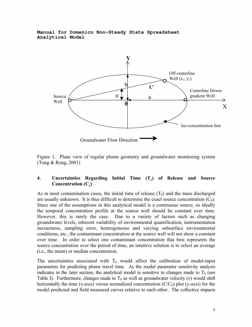
E. Model prediction and solutions are presented in Cell B14-B19, and in CellC14-C18. Record the times at which the MTBE plume front first appears(i.e., when MTBE concentration is greater 5 µg/L). The time is shown in CellB16 (days) and C16 (years). The maximum MTBE concentration predicted toappear in the drinking water well and the associated time at which it appearsis shown in Cell B19 (µg/L) and C17 (years), respectively. Cell C18 showsthe time (years) remaining for the plume to reach 5 µg/L in the drinking waterwell. The Microsoft Excel worksheet shows that given the monitoring data atMW-6, it would take approximately 25.8 and 37.0 years for the MTBE plumeto travel to and reach maximum concentration, respectively, in thedowngradient drinking water well 1,000 feet away. An approximate estimatefor this time can also be obtained through visualizing Figure 4 in Excel file.

F. Save the file.

9. Troubleshooting for the Spreadsheet Analytical Model

Trouble 1: By changing the values of either αx, ν, or λ, the model calculation and curveon the chart do not respond.

Solution: Go to “Add-In” option in Excel under the “Tools” menu bar and select the“Analysis Toolpak.”

Trouble 2: Some field data do not show on the chart.

Solution: Change the Y-axis range by double clicking the Y-axis, and add one or two moredecimals for minimum range in Scale sheet.

Trouble 3: The predicted plume travel times do not show on the chart.

Solution: Change the X-axis range by double clicking the X-axis, and add one or more digits for maximum range in Scale sheet.


17

10. Acknowledgments

The authors would like to thank David Bacharowski of the Los Angeles Regional WaterQuality Control Board for his constructive criticism and support in the development of thiswork.

11. References

AT123D, Reference Guide and User’s Guide (Version 3.0), (1998). General SciencesCorporation, 4600 Powder Mill Road, Suite 400, Beltsville, MD 20705.

Bouwer H (1978). Groundwater Hydrology. McGraw-Hill Book, New York, 448 pp.

Dawson KJ and Istok JD (1991). Aquifer Testing – Design and Analysis of Pumping andSlug Tests. Lewis Publishers. Chelsea. 344 pp.

Domenico PA and Robbins GA (1985). A new method of contaminant plume analysis.Ground Water 23(4): 476-485.

Domenico PA (1987). An analytical model for multidimensional transport of decayingcontaminant species. Journal of Hydrology 91: 49-58.

Environmental Resolutions, Inc. (2001). Quarterly Groundwater Monitoring Report –Fourth Quarter 2000.

Freeze RA and Cherry JA (1979). Groundwater. Prentice-Hall, Inc., Englewood Cliffs, NJ07632. 604 pp.

Fried JJ (1975). Developments in Water Science. Groundwater Pollution: Theory,Methodology, Modeling and Practical Rules. American Elsevier, New York, 132 pp.

Gelhar LW and Axness CL (1981). Stochastic analysis of macrodispersion in three-dimensionally heterogeneous aquifers. Report H-8. Hydraulic Research Program. NewMexico Institute of Mining and Technology, Socorro, NM 87801.

Gelhar LW, Welty C, and Rehfeldt KR (1992). A critical review of data on field-scaledispersion in aquifers. Water Resources Research 28(7):1955-1974.

Martin-Hayden JM and Robbins GA (1997). Plume distortion and apparent attenuation dueto concentration averaging in monitoring wells. Ground Water 35(2):339-346.


18

Rong Y, Wang RF, and Chou R (1998). Monte Carlo simulation for a groundwater mixingmodel in soil remediation of tetrachloroethylene. Journal of Soil Contamination7(1):87-102.

Roscoe Moss Company (1990). Handbook of Ground Water Development. John Wiley andSons, New York. 493 pp.

Todd DK (1980). Ground Water Hydrology. John Wiley and Sons, New York.

Tong W and Rong Y (2001). Estimation of Methyl tert-Butyl Ether Plume Length Using theDomenico Analytical Model. Journal of Environmental Forensics 2(3), Article No.enfo. 2001.0025.

United States Environmental Protection Agency (USEPA), (1996). Soil screening guidance:technical background document E-25pp EPA/540/R-95/128, PB96-963502.

Documents

Preface To Manual For Domenico Non-Steady State Spreadsheet Analytical Model