preface - · PDF filepreface The work presented in this thesis has ... project. The work done on face ... proach this goal by investigating statistical diﬀerences in two sets of

preface

The work presented in this thesis has been funded by the BIOP (BiomedicalOptics and New Laser Systems) graduate school.

The project originally consisted of two parts, namely reconstruction of theretina (in collaboration with the Department of Ophthalmology at HerlevHospital) and modelling of the human face. After some initial work on theretina project (literature overview and blood vessel segmentation) it wasdiscontinued, and instead focus was directed solely on the face modellingproject.

The work done on face modelling, have resulted in articles on registrationand shape modelling, and in the release of open source software deliveringa framework for rendering, segmenting and tracking of 3D objects in 2Dimages.

This hopefully enables students to investigate these fields and continue theconstruction of a general 3D scene modelling system.

acknowledgements

Lunds Institute of Technology is greatly acknowledged for the matriculation,as are the kind people at the Centre for Mathematical Sciences in Lund aswell as the Danish counterpart at the Image Analysis and Computer Graph-ics group at the Department of Informatics and Mathematical Modelling atDTU.

My supervisors, Kalle Astrom and Rasmus Larsen, are thanked for their pa-tience and advises while guiding a stubborn student through to the deliveryof this Licentiate thesis.

I am especially indebted to the BIOP graduate school for the financing of theproject, and the 3D-laboratory at the School of Dentistry at the Universityof Copenhagen is thanked for letting me use their scanning equipment.

A special gratitude for a plain lovely atmosphere goes to my roommate atLTH, Johan Nilsson. Finally I would like to extend these appreciations toinclude my friends and family, love to all.

i

ii

ii

Contents

1 introduction 1

1.1 layout of thesis . . . . . . . . . . . . . . . . . . . . . . . . . . 4

1.2 contributions . . . . . . . . . . . . . . . . . . . . . . . . . . . 5

2 data 7

2.1 acquired shape data . . . . . . . . . . . . . . . . . . . . . . . 8

2.2 acquired texture data . . . . . . . . . . . . . . . . . . . . . . 12

3 registration 13

3.1 registration of expression shapes . . . . . . . . . . . . . . . . 16

3.2 registration of ID shapes . . . . . . . . . . . . . . . . . . . . . 25

4 model 27

4.1 3D shape model . . . . . . . . . . . . . . . . . . . . . . . . . . 28

4.1.1 expression shape model . . . . . . . . . . . . . . . . . 28

4.1.2 ID size & shape model . . . . . . . . . . . . . . . . . . 34

4.1.3 applying expressions to IDs . . . . . . . . . . . . . . . 37

4.1.4 reducing number of vertices in model . . . . . . . . . . 39

4.2 texture model . . . . . . . . . . . . . . . . . . . . . . . . . . . 40

4.3 rendering . . . . . . . . . . . . . . . . . . . . . . . . . . . . . 42

4.3.1 light model . . . . . . . . . . . . . . . . . . . . . . . . 45

4.3.2 analytical Jacobian . . . . . . . . . . . . . . . . . . . . 49

4.3.3 analytical Jacobian vs. numerical Jacobian . . . . . . 54

5 segmentation 55

5.1 optimising . . . . . . . . . . . . . . . . . . . . . . . . . . . . . 55

5.1.1 optimising near (a) minima . . . . . . . . . . . . . . . 55

5.1.2 position initialisation . . . . . . . . . . . . . . . . . . . 56

iii

iv

5.2 automatic artificial active appearance model (AAAAM) . . . 58

5.3 segmentation of faces in images . . . . . . . . . . . . . . . . . 62

5.3.1 segmentation of pose, selecting variability . . . . . . . 62

5.3.2 segmentation of ID and frontal pose . . . . . . . . . . 67

5.3.3 segmentation of ID and profile pose . . . . . . . . . . 70

5.3.4 segmentation of ID and a smile expression . . . . . . . 73

5.3.5 segmentation of ID, pose, lights and random expression 76

6 conclusion 81

6.1 future work . . . . . . . . . . . . . . . . . . . . . . . . . . . . 82

6.1.1 object features . . . . . . . . . . . . . . . . . . . . . . 82

6.1.2 sub-models . . . . . . . . . . . . . . . . . . . . . . . . 82

6.1.3 automatic model expansion and learning . . . . . . . . 83

6.1.4 databases . . . . . . . . . . . . . . . . . . . . . . . . . 83

6.1.5 databases of other objects . . . . . . . . . . . . . . . . 84

Bibliography 85

A appendix 93

A.1 concepts, used rutines and formulas . . . . . . . . . . . . . . . 94

A.1.1 principal component analysis . . . . . . . . . . . . . . 94

A.1.2 barycentric coordiantes . . . . . . . . . . . . . . . . . 94

A.1.3 isometric mapping . . . . . . . . . . . . . . . . . . . . 95

A.1.4 model view matrix and quaternions . . . . . . . . . . 96

A.2 data . . . . . . . . . . . . . . . . . . . . . . . . . . . . . . . . 97

A.2.1 nonregistered ID . . . . . . . . . . . . . . . . . . . . . 97

A.2.2 nonregistered expression . . . . . . . . . . . . . . . . . 99

A.2.3 registered expression . . . . . . . . . . . . . . . . . . . 102

A.2.4 registered ID . . . . . . . . . . . . . . . . . . . . . . . 105

A.3 IMM face database images . . . . . . . . . . . . . . . . . . . . 107

A.4 threedit . . . . . . . . . . . . . . . . . . . . . . . . . . . . . . 112

A.4.1 Octave rendering and 3D object segmentation software 112

iv

v

A.4.2 3D shape editor . . . . . . . . . . . . . . . . . . . . . . 114

A.4.3 texture coordinate editor . . . . . . . . . . . . . . . . 115

A.4.4 triangulator . . . . . . . . . . . . . . . . . . . . . . . . 116

A.4.5 registrator . . . . . . . . . . . . . . . . . . . . . . . . . 117

v

CHAPTER 1

introduction

’What’s that?’, not the expected question when a human is presented with apicture of a face, because we recognise faces instantly and almost regardlessof pose, the light conditions, facial expressions and most artifacts. But it isstill an essential question when the same image is presented to a computer,and the answer from such a machine may vary a lot.

The basic idea of asking machines what’s in an image, is to supply machineswith vision, a highly desired ability as we move along the path of integratingand interacting more and more with machines in our every day life. Onceour interaction with these machines reach a higher level, than eg. typing ona terminal, it may be of utmost importance that they are able to recognisehuman form, human identity and their dynamic expressions.

Here we’ll investigate what is required in the construction of a face segmen-tation systema, capable of handling large and natural occurring differencesin pose, light and shape variations (expression and ID for faces). We’ll ap-proach this goal by investigating statistical differences in two sets of 3D facialsurface recordings. One set capturing ID variations and one set capturingother facial surface deformations, ie. expression variations. The results ofthese analyses will be incorporated into a 3D facial segmentation system,handling ID, expression, facial texture variations, lighting conditions andhead pose.

Ie. we’ll try to construct a system capable of answering questions such as’what is the pose of the face?’, ’what are the light conditions?’, ’what isthe ID?’, ’what is the expression?’ and ’what is the texture like?’. Wewill be assuming that there actually is a face present in the images which wesegment, so we are not addressing the question ’is there a face in this image?’.

aActually we are constructing a general 3D object segmentation system, but we’ll focuson human faces.

1

2 introduction

Most of the face segmentation research, have tried to answer such questionsby methods based on 2D image data machine learning algorithms. The pi-oneering work by Turk and Pentland named eigenfaces (33), (34) initiated alot of research in the usage of PCA (principal component analysis) for imageanalysis and specifically in the areas of medical image analysis, face recog-nition and feature description.Popular and widely used methods which utilises this projection approach in-cludes AAM (active appearance models) by Cootes et al. (2),(23),(24),(21),(22)

along with the many AAM variants, and improvements, as reported by thegroup of Matthews and Baker in (32), where they introduce the concept ofinverse compositional image alignment (ICIA), which improves AAM opti-misation (its noted that (45) corrects some errors in the original ICIA paper).In (29) they show how to constrain the 2D AAM search by valid 3D modelmodes. In (30) occlusion handling in 2D AAM are addressed, and in (31) and(28) they investigates improvements with person specific AAMs as well as ro-bustness improvements as achieved by fitting multiple images with a singleAAM.

Other popular statistical methods like ICA (independent component analy-sis), LDA (linear discriminant analysis, aka fisherfaces), Isomapping, kernelmethods, HMMs (Hidden Markov Models) and SVM (support vector ma-chines) have likewise all been applied to the analysis (global recognition andlocal feature description) of face data.

Most researchers have focused on face recognition (or maybe this should berefrased to; most funding agencies have been focusing on face recognition)and most of the before-mentioned methods have resulted in good results.SVM shows good performance even for significant pose differences, eg. (35),PCA and ICA have been extensively explored also with good results reportedby eg. (17), (18) and (22).

For emotion and expression recognition, most algorithms concentrate onnon-static methods, ie they use dynamic data from video, and utilise theinformation available in optical flow computations to drive some 2D or 3Dmodel, and classify the registered expression by use of the FACS (Facial Ac-tion Coding System (72), the animation-parameters which are also used inmpeg4 video compression). This is done on 2D dynamic image sequences byeg. (15), (12), (13). HHMs are used in eg. (10) and (11). ICA and other methodsfor this facial action classification are explored by eg. (16), and of-course theusage of AAMs have been explored, by eg. (20).

To construct a system which is capable of handling all of the obstacles intro-

2

introduction 3

duced in real world images, ie large deviations in pose, light and expressionconditions, it seems to be necessary to introduce a more complete model ofthe face. Ie to model the actual 3D surface of the object along with the vi-sual variabilities observed from variations introduced by gender, age, weight,ID, expression, race, face-features or skin textures such as hair, pimples, cos-metic, jewelry, as well as the head pose and the light position and type, plusthe resulting cast shadows.

One of the first 3D face models were build by Parke and Waters in the earlyseventies (64), their approach was to build a simplified muscle model of theface. This was later extended to include more facial tissue layers and moremuscles (73). Such a physical muscle based model approach, give the advan-tage of well controlled surface deformations (from manually defined actioncodings) resulting in a wide and controllable range of variability in both ex-pressions and ID. A successfully implementation of this approach have beenachieved by Alhberg et al. with the Candide model, (7), (6),(5) and (4) show-ing fast, and, what seems to be, good and accurate results. Another musclemodel implementation showing the strength of this approach is by Lee (8)

who builded a second order ODE model.

The emergence of apperature enabling precise and fast 3D surface record-ings, initiated the construction of new models, utilising real world data andemerging machine learning algorithms. These new models are the statisti-cally driven models, as seen in the PCA based 3D morphable models by theBlanz and Vetter grouph, (41), and the point distribution models by Huttonet al. (39).

State of the art in 3D face modelling (focusing on realistic looking faces, notrecognition or other sort of classification results) are, I believe, achieved byBlanz and Vetter eg. (41),(42),(43),(44).

Once the model frame-work have been established, most researchers use theirmodels to segment faces in 2D images. The task of segmentation requiresa fitting algorithm, in which the model parameters are guided towards theoptimal values, in the sense of minimising some score function. Most fittingalgorithms are constructed in order to full-fill the requirements of any goodalgorithm, namely being automatic, robust, accurate and potentially fast.Since we are evaluating a analytical expression for the model Jacobian, we’llbe using a numerical optimisation method which uses this Jacobian.The two main 3D face models by Blanz-Vetter and Ahlberg respectively, uses

3

4 introduction

different cost functions and different optimisation techniques in their fittingalgorithms. The Blanz and Vetter grouph uses a stochastic gradient descentmethod, on a random subsets of the model triangles, using a maximum aposteriori estimator (MAP) as cost function. They divide their model intofour sub-model which they optimise separately. In their articles (41) and (42)

they obtain impressive segmentation results, but reports slow convergences.In (44) they introduce a regularization term penalising low probability solu-tions and uses dynamical weights on the sum of feature point error (featurepoints picked by user) and image model error. Romdhani and Vetter intro-duces a smoother cost function in (46), where they add edge features andspecular highlight features, resulting in a new fitting algorithm which theyterm the Multi-Feature Fitting algorithm. They obtain a more robust anda faster segmentation algorithm, but they do not obtain real-time fitting.

For a real-time, and what seems to be a robust, algorithm we turn our at-tention to the Ahlberg 3D face model. In (6) Dornaika and Ahlberg presentsa two step algorithm in which they apply a global RANSAC method to es-timate the rigid motion of the head in-between video images (the RANSACpart estimates 3D model to 2D image point correspondences using pointswhich are affected by rigid motion only), and a local optimisation scheme toestimate the facial animation parameters. The local adaption of the modelparameters is done by using a ’traditional’ AAM search concept, where re-lation and update matrices are constructed in advance from known exampleimages.

1.1 layout of thesis

In this thesis we’ll first look at data collection and some necessary manualdata editing. Next we’ll investigate howto registrate 3D shapes, and com-ment on how other groups have addressed this problem. We’ll focus our efforton the registration of deformed 3D surfaces and introduce a new algorithmto register these. Non-deformed surfaces (scans with neutral expression)are registered in a standard fashion, with manual selected landmarks pointswarped onto a default shape, followed by a closest surface point registration(searching in the direction of the surface normal).

After registration we are ready for the model constructions, where we buildtwo independent models, one shape model for the expression data and onesize & shape model for the ID data. The resulting model is textured with a

4

1.2 contributions 5

texture model constructed from a public face data base.

Hereafter we construct rendering software for the Octave program, includingthe Phong illumination model, and present the analytical Jacobian of theresulting rendered 2D image, dependent on model parameters controllingexpression, ID, phong light parameters and model pose.

Finally we investigate the system performance when segmenting faces in 2Dimages. In the segmentation part we first introduce the concept of automaticartificial active appearance models (AAAAM) for the initial parameter es-timation, followed by the global optimisation in the full 3D realm. Next weinvestigate the performance for pose estimation and expand the segmenta-tion to combinations of pose, ID, expression and light.

We end up with a conclusion on the project as a whole and describe a fewof the required and desired possibilities for improvements and further inves-tigations, ie. future work.

1.2 contributions

During the course of this project, a program package which enables the ren-dering, modelling and segmentation of 3D forms have been constructed. Thissoftware package, along with some editing programs, are published as opensource for the interested user or student.

Apart from the open source software, a few articles discussing different partsof the problems investigated have been published in conference papers. Theseincludes;

• R. Larsen, B. Lading, Multiple Geodesic Distance Based Registration of

Surfaces Applied to Facial Expression Data, International Symposiumon Signals, Circuits and Systems (ISSCS) 2007., vol. 1, IEEE, 2007

• B. Lading, R. Larsen, K. Astrom, 3D Face Appearance Model, Pro-ceedings of the 7th Nordic Signal Processing Symposium (NORSIG),University of Iceland, 2006

5

6 introduction

• R. Larsen, K. B. Hilger, K. Skoglund, S. Darkner, R. R. Paulsen, M.B. Stegmann, B. Lading, H. Thodberg, H. Eiriksson, Some Issues of

Biological Shape Modelling with Applications, 13th Scandinavian Con-ference on Image Analysis (SCIA), Gothenburg, Sweden, vol. 2749,pp. 509-519, Springer, 2003

• K. Skoglund, R. Larsen, B. Lading, Building a 3-D Appearance Model

of the Human Face, DSAGM, DIKU , 2003

6

CHAPTER 2

data

In order to construct a physical meaningful model of a physical object, orphenomena, we need observations of the variables and measurements of thedependent parameters. For a 3D face model, we need observations of surfacepoints, which in-turn enables us to build a polygonal surface representationof the object. As for dependent parameters, it would be desirable to haveknowledge of skin characteristics influencing the intensity representation inthe 2D RGB image. These parameters are not available and must thereforbe estimated as we go along.

For the recording of the 3D point positions, we have used a Minolta Vivid900 laser scanner, situated at the 3D-laboratory at the School of Dentistryat the University of Copenhagen. This system works on a principle of lasertriangulation combined with a colour CCD image. The scanner directs itslaser on the object and the laser mark is registered in the CCD camera. Sincethe distance between the camera and the laser is known (both are internallyfixed) a triangulation may be carried out to calculate the 3D position of thelaser dot. To speed up the scanning procedure, the Minolta Vivid scannersweeps a laser stripe across the object, instead of a single laser dot.

The internal monochrome CCD camera has a resolution of 640× 480 pixels,and RGB images are obtained by adding red green and blue filters in frontof the camera. The accuracy of the registered 3D Euclidean coordinates are,officially, in the range; x = ±0.22mm, y = ±0.16mm and for the depthz = ±0.1mm.

Since a single scan takes a few seconds (≈ 5s), the object must be absolutelystill and attain a pose and expression which is stable for the duration of thescan. To obtain a full surface representation with no occlusions, several scansare required. With three scans (one at 0o and two at ±30o) the whole face in-cluding the chin, nostrils, cheeks and the sides of the nose are recorded. Thethree scans are combined using software supplied with the Minolta scanner.This scanning procedure is used for all scans where the object can maintain

7

8 data

the expression, which was only achieved in the case of a neutral expression.For scanning facial expressions/perturbations this merging approach was nota workable solution, therefor all scans involving expression/perturbation aredone with a single frontal scan.

The main drawback of this scanning technology, is the time required to obtaina single scan (plus the poor 2D image quality), this results in difficulties whenscanning a perturbed state, and it makes the capture of true expressions(captured in a emotional expression sequence) impossible. To obtain datawhich accurately records the surface during such a sequence, better scanningequipment have to be applied. Among candidates whom seems to delivergood 3D scans and textures are Cyberware (67) (used by the Blanz andVetter group) and Breuckmann’s facescan III (68) (the latter uses structuredlight while the cyberware scanner uses triangulation of laser). It is notedthat this is an emergent marked and that a lot of new 3D scanning productsare being introduced.

2.1 acquired shape data

We have scanned 24 individuals with neutral expression. These scanned sub-jects range in age from 5 to 40, both males and females. Most scannings wereof males age 25− 30 of Scandinavian origin. For the expression database wehave collected 35 scans of different facial-muscle perturbations of the sameID, namely the author. The limited variability in both databases, constraintsthe explored face-space and thus the constructed model.

In figure 2.1 two samples from the ID-database are shown. As seen in thetwo lower figures the alignment procedure (the one included in the Minoltasoftware) produces undesirable artifacts such as triple lips. Such artifactsare not edited, but are somewhat suppressed in the final registered shapes.All ID-shapes has some small holes, either caused by occlusion, diffuse re-flection on wet or hairy surfaces, or internally in the Minolta software whenthe three recorded shapes are aligned. These holes and other artifacts wereedited in the Minolta software (as well as in home made editing programs).All 24 raw recordings are shown in figures A.1 and A.2 in appendix A.2.1

During all recordings two light sources with reflectors were setup to ensurean ambient lit scene. This was done in order to get better texture, but asis evident in figure 2.2, where the recorded texture is mapped onto the twosurfaces, the texture is of poor quality. This seems to be due to a bad green

8

2.1 acquired shape data 9

Figure 2.1 Merged scans of different ids with neutral expression. The mod-els consists of approximately 23000 vertices and 24000 polygons.Notice the ’triple-lips’ artifact which is introduced by the scanningsoftware.

Figure 2.2 Same models as in figure 2.1, here with the recorded textures.

9

10 data

colour channel.

Figure 2.3 Two scans from the expression database. The size of the modelsare typically 10000 vertices and polygons. In the bottom row thescanned models are shown with the scanned texture.

In figure 2.3 two shapes from the expression-database are shown. The firstshape is a very good recording, whereas the second shape has some parts ofthe chin and the cheeks occluded, causing it to be discarded.

All expression data is edited. Recordings which have errors at the eyelashesare edited such that these are suppressed, and the resulting surface aroundthe eye is more elliptical. The mouth region is edited in all expression shapes,such that the lips are separated (this was necessary in order to estimate the

10

2.1 acquired shape data 11

geodesic distance between points), and in some of the shapes, the regionsdefining the eyebrows and the nostrils were also edited. Furthermore allshapes have been reduced to only cover a defined region of interest (thisregion is partly defined by the surface area which all acceptable recordingscovers). In figure 2.4 we show an example of an edited shape.

Figure 2.4 A sample from the expression database, before and after the initialediting.

All edited expressions are edited with homegrown software, which enablesthe user to mark and delete regions of points, mark one or multiple pointsand move or delete these, add triangles and delete triangles as well as split-ting adjacent triangles and reducing the number of vertices and smoothingthe mesh. Some screenshots and further information of this editing softwareis avaiable in the appendix section A.4.

11

12 data

2.2 acquired texture data

As mentioned the acquired textures are not useable and we therefore needa new texture in order to texture our model. A set of images of the author(the subject for the expression database) with normal expression was takenunder diffuse light, a single image was chosen and edited (eg. reflections ineyes removed).

Figure 2.5 Screen shots of the texture coordinate constructor program. Theshown texture is the chosen default texture.

In figure 2.5 the program used for the construction of texture coordinatesis shown. Points on the 3D model are chosen and kept fixed, correspond-ing points are added, in the same order, in the 2D texture image, and aTPS (thin plate spline) warping is applied. Once the texture is mapped,fine-tuning may be done, where points in the 2D image can be moved inter-actively. We have used 5 to 10 mappings for each model size (large, mediumand minimal) and chosen the best one (based on visual inspection) as thedefault texture coordinates.

To include variability in the texture, we use the ’IMM Face Database’ (36),which consists of six sets of face images of 40 different people. The set usedfor the texture model, is 40 full frontal face images with neutral expressionand diffuse light. Some of the other sets are with a frontal ’happy’ expression,a rotation set and a set with neutral expression and spot light. These addi-tional data sets will be used to test the model in the segmentation section5.3.

12

CHAPTER 3

registration

Registering shapes consisting of connected points in 3D Euclidean space, ispart of the correspondence problem, where we wish to locate correspondingpoints on different surface scannings. Ie on the surface patch σ belonging tothe template shape, we have certain node points defining our vertices of thepolygonal mesh, these node points must have a match on the surface of theother shapes.

This correspondence problem becomes very difficult to solve when operatingon surfaces with large deformations and foldings. As is encountered in ourexpression database.

A ’traditional’ way to establish correspondences between points on all shapes,is to manually pick some easily recognisable landmark points, eg. nose-tipand corners of the eyes for face shapes. Once a small set of such landmarkpoints have been selected, dense correspondence is obtained by interpolationbetween the landmarks. This approach is applicable for shapes with lim-ited deformations, where a warping with TPS (Thin Plate Spline) gives anadequate and smooth interpolation between landmarks. Such an approachhave been used by eg. Hutton (38) for registration of 3D faces, in a modifiedversion where Active Shape Models (ASM) (74) are constructed and works ina hybrid with the all-round registration and alignment tool, Iterated ClosestPoints (ICP) (70).

For shapes with large surface deformations, such as foldings, this approach isnot adequate, since a TPS-warp of a sparse set of landmarks, does not repro-duce foldings and other large surface deformations in-between the landmarks.

Since we are working with 3D surfaces, we may utilise functions which de-scribe the local surface properties, such as the surface normal and local cur-vatures (mean and Gaussian curvature). But such local surface descriptorsare only applicable in corresponding regions with no surface deformation.

13

14 registration

Among other local descriptor choices we have the ’shape context’ descriptorby Belongie et al (51), where each data point is assigned a descriptor, describ-ing the density and distribution of points in its neighbourhood. Consider aplane surface patch and its deformed/folded state; the undeformed patch willresult in a shape context histogram very different from the one obtained bythe folded patch (in the article (51) they consider 2D shapes, and constructshape contexts by counting shape points in a 2D log-polar histogram. Fora 3D shape we would construct a log-polar-sphere histogram). For the un-folded surface patch we would only count samples in one sphere-intersection,while its folded counterpart would result in non-empty bins across sphere-intersections. Above mentioned shape-descriptors are therefor, probably, notapplicable for the registration of our deformed surfaces.

Working with image data, a fundamental information aught to be the inten-sity values of the different image bands. But the applied textures and theapplied texture coordinates need to be of good quality in order to do a decentjob with this information. As seen in chapter 2 this is unfortunately not thesituation. If recordings where done with coloured markers distributed acrossthe surface of the scanned face (and if the texture samples captured this in-formation), we might had obtained a subset of textures and mappings withgood correspondence information. A quick study of the applied textures infigures 2.3 shows that there is no useable information (data is missing) tobe had in the deformable regions (true for most samples of the expressiondatabase).

In some of the most successful work done on 3D face registration and mod-elling, eg. articles driven by Blanz and Vetter (41) (42) and (43), the registrationprocess is utilising the red, green and blue components of the textures, to-gether with cylindrical coordinates of the recorded points. They implementa modified optical flow algorithm resulting in impressive registrations. In (41)

all data is focused on different IDs (100 males and 100 females), and in (44)

the focus is on different mouth shapes and facial expression (35 samples),where the recorded subject has fiducial markers and lipstick to increase per-formance for alignment and for better lip contrast. Their recordings weredone with a Cyberware scanner (uses laser triangulation and scanning a full360o). They register the 200 neutral faces in an automatic manner (neutralexpressions means that there are no foldings, no deformations), but uses aniterative manual bootstrapping method for the deformed expression shapes.

For deformed surfaces we have one descriptor which is invariant to bending

14

registration 15

and deformations (as long as these deformations does not stretch the sur-face), this is the geodesic distance between points on a surface patch. Thisdistance measure have been used with success to register highly curved andfolded surfaces such as 3D brain scans, see eg. (48) where they minimise anobjective function combining geodesic distance with the surface normal andcurvature (Gaussian- and mean surface- curvatures), achieving what lookslike nice registrations (it is however very difficult for an untrained eye toobserve false registration artifacts on curly objects as brains).

Another use of geodesic distance for registration, is reported in the workby Bronstein twins and Kimmel (52) (53) (54), where each recorded face sur-face is mapped into, what they term, the ’bending-invariant canonical form’(this mapping is identical to the Isomap procedure proposed by Tenenbaumet al (55)). After mapping all surfaces into this isometric space, they use’standard rigid surface matching methods’ for the matching (these standardmethods is presumably Procrustes together with ICP). They use a precisegeodesic path computation method, which was suggested by Kimmel (56) and(57).

Another approach to obtain good registrations is by optimising some measureof model quality. One measure of model quality could be the Minimum De-scription Length (MDL), see eg. (25) (26) (27) and (58). In such an approach aninitial registration is iteratively improved (in the sense of minimising MDL)by perturbing points under some (or none) constraints. These constraintsmay include point inter-distances and local curve/surface properties. In (27)

they work on 3D shapes (brain ventricles and rat kidneys), and optimise theresulting shape model by optimising the parameterisations of the shapes.They are able to define an explicit representation of the parameterisationsby mapping each surface point onto a sphere (assuming that the surface istopologically equivalent to a sphere). These mappings are homeomorphicmappings (continuous, one-to-one and onto) of the sphere. For facial sur-faces with foldings (as the cheeks in a smile) the mapping onto a sphere willnot be one-to-one, and this mapping method will most likely not be usefullfor our data.

Other interesting methods includes an approach suggested by Nielsen etal. (49), who solves the correspondence problem by solving a geometry con-strainted diffusion problem. They obtain nice looking (visually they obtaina nice grid, and they conclude that they are able to explain more of theobserved variance) results on 3D mandibles data.

15

16 registration

3.1 registration of expression shapes

For the registration we choose a template shape, which all other shapes, bothID and expression, are registered to. The chosen shape is shown in figure3.1.

Figure 3.1 The default template shape with landmarks, and numbered se-quence.

This template shape has an, almost, neutral expression, its polygonal gridis regular and the surface is smooth. In the figure we also show the thirteenlandmarks. These landmarks are manually placed on all shapes (both ID andexpression). Selection of the landmarks is restricted to the recorded points,ie we have not picked landmarks on the surface but on the recorded grid.This restriction results in some initial errors which are progressed through-out the registration procedure.We have tried to minimise these manually placed landmark errors by iter-atively perturbing a landmark position and minimising the resulting MDLscore (where PCA was done on the landmark point sets only). This resultedin a collapse of the landmarks, eg. landmarks number 4 and 5 moved towardslandmark 6 or 7. Constraints on the displacement from the initial positionwas applied (points was not allowed to move more than two times the meanlength of the edges) but the resulting placement of the landmarks did notsatisfy an investigating eye (it was clearly visible that landmarks did notcorrespond). We therefor keep the manually placed landmarks.

In the ’traditional’ registration routine, we apply a TPS to the template land-

16

3.1 registration of expression shapes 17

Figure 3.2 A shape registered in the ’traditional’ way. Top left is the raw(edited) data, top right the registered and in the bottom row weshow a closeup of the troublesome region.

17

18 registration

marks and warp them onto the landmarks of the new unregistered shape.The warp transform is then applied to the full template shape, and a closestsurface point registration produces the final registered shape. In figure 3.2 weshow a sample of the expression data at the top left, and the registered ver-sion to the top right. Overall we have obtained a visually good registration,the nose-, eyes-, chin- and mouth-regions are all registered nicely. In the bot-tom row, of figure 3.2, we have a closeup on the troublesome region. As seenthis ’traditional’ routine does not produce satisfactory results at foldings.The deformed surface is not registered correctly, points collapse and the gridbecomes unevenly distributed. These undesired effects could be suppressedby applying more landmarks, but we do need quite a few ekstra landmarksin order to obtain a correct warp, and these landmarks will all be located inthe same neighbourhood (and they will all add up on the errors introducedin manual landmarking) which results in a poor TPS transform. This ekstralandmarking approach is commented in the end of this chapter, see figure 3.9.

To overcome some of these artifacts, we map our data into spaces wherefolded and deformed surfaces are not as expressive as in the Euclidean space.One such mapping is obtained by plotting our surface in a geodesic distancespace. Ie. first we calculate the geodesic distance matrix, Dg, where entryDg(i, j) is the estimated geodesic distancea between point i and point j.Next we pick three landmarks, A,B and C, and map all Euclidean coordi-nates into the geodesic distance space defined by these landmarks, such thatfor node i the mapped coordinates are; xi → Dg(i, A), yi → Dg(i, B) andzi → Dg(i, C). In figure 3.3 three of these resulting mappings are shown forthree different shapes. As seen we obtain very different surface representa-tions, while the shape seems similar in each mapping. In the last row wehave shown the shapes obtained after an isometric mapping.

For each of the three geodesic mapping representations, we apply TPS-warping and closest surface point registration, and end up with three differ-ent registrations of each shape in the geodesic distance space. Each pointregistration is mapped back to Euclidean space by recording the registeredpoint triangle id and its barycentric coordinates. In addition to the threegeodesic distance registrations we also have the default Euclidean registra-tion, resulting in four registered surfaces for each recorded shape. The reg-istered shapes (the three geodesic mappings and the isometric) are show infigure 3.4.None of these registrations are found to be optimal, and the last one (from

aThe geodesic distance between points are estimated as the shortest path along theedges of the model, using Floyd’s algorithm.

18


Figure 3.3 The template shape and two expression shapes in the mappedspaces. From top to bottom; Euclidean, geodesic (0, 1, 3),geodesic (0, 1, 6), geodesic (0, 1, 8) and isometric.

19

20 registration

Figure 3.4 Two different registered shapes in each column. Bottom row isregistration from isometric mapping, others are from the geodesicmappings as seen in figure 3.3.

20


the isometric mapping) is of no use at all (we also observe that in figure3.3, the shapes from the isometric mapping differs too much in form, eg.the forehead), and is therefor discarded in the final registration. We endup with four representations of each shape. The original Euclidean and thethree shapes in geodesic space.All registrations done in the geodesic mappings, proves to be very good atregistrating the folded areas, but they differ significantly in areas like theforehead.

As seen from these registrations, we are in need of some method to evaluateand assign each of the final registrated points. Different procedures have beentested, where each registered point is given a registration score, based on theregistration point-to-surface distance, the bounding box and a geodesic score;

distance score is normalised squared Euclidean distance from (warped)template point to registered surface point. A normalisation is done bydividing with the distance between landmarks 0 and 1.

bounding box score (even grid) is calculated for each triangle on theregistered shape and on the template shape, the length of the diag-onal of the triangle bounding box is calculated. These are summed

up to give a weight on each point Wbbox =P

i bbox regiP

i bbox meani, where

summation is done over all cells connected to the current point.

geodesic score (global position) is based on the geodesic distance to theset of landmarks used for the mapping, normalised with the geodesicdistance between landmarks 0 and 1; di,l = Dg(i, l)/Dg(0, 1), whereDg is the matrix with geodesic distances, i is the point id and l islandmark id. For each registered point di,l is calculated for the meanshape and for the three points of the triangle in which the registeredpoint resides (dα

i,l, dβi,l and dγ

i,l) on the unregistered shape. These scoresare summed up over all landmarks

geodesic scorei =

∣∣∣∣∣

1

N

l=N∑

l=1

di,l

(dαi,l + dβ

i,l + dγi,l)/3

∣∣∣∣∣.

These registration scores all provide useful information on bad registered ar-eas. They all seems (when texturing the surface with the scores) to be goodmeasures, and registration procedures which combines these scores (sums upover nearest neighbours, iteratively registrates and recalculates the scores)have been running in any possible mode, with no luck at all. All registra-tions have resulted in visual obvious errors, bad mesh quality, overlapping

21

22 registration

mesh regions and other obvious false registration artifacts. The problem incombining the different registered meshes is, often, that the surfaces appearsin kinks and overlapping meshes.

The final registration is done without any score function (due to the difficul-ties in combining the meshes). We find the best results by simply recordingthe mean of the four registered points as the Euclidean coordinates of thefinal registration! Iff this mean does not look good, we rerun the registra-tion procedure and discard one point at each point registration, namely thepoint which diverges most from the mean (ie largest Euclidean distance).Discarding points was done in a few, three to five, registrations.

In figure 3.5 we show the final registration result, and a zoom-in on thetroublesome region. As seen we have obtained an acceptable registration,the deformed area is nice and smooth and the overall impression is good.Comparing this registration with the registration in figure 3.2, we observethat the lips and its local region and the chin are better registered in the’traditional’ registration, but all artifacts are reduced significantly in the fi-nal registration.

Figure 3.5 Final registration. Same shape as in figure 3.2.

Using this registration routine, we register 31 of the 35 expression shapes(shown in figures A.6 and A.7 in appendix A.2.3). This leaves four uneditedexpression shapes unregistered. These shapes are ’leave-out’-shapes for thetesting of an semi-automatic registration routine (’semi’ due to the necessityof supplied landmarks).

This routine first aligns all registered shapes (with a similarity transforma-tion) and builds an initial statistical shape model (SSM). The mean shapefrom this model is TPS-warped onto the new surface and the first registration

22


is done. The model is then used to find the parameters which best expressesthe variation between the mean and the newly registered shape. Applyingthese parameters to the model followed by a new registration, we obtain ashape which is added to the model. Once added we iteratively build the SSMmodel, compute closest match, register and reassign until no improvementsis achieved (based on the sum of the registrated point to surface distances).

Figure 3.6 Semi-automatic registration of unedited ’leave-out’ samples. Toprow is ’unseen’ and unedited shapes, middle row is registeredwith the automatic registration routine. Bottom row is zoom-inon some of the troublesome areas.

In figure 3.6 we show the registration result of the semi-automatic registra-tion routine. We observe good registration results with evenly spaced polyg-onal grids, but notice that the border areas around the lips are still troubled.

The automatic routine was also used to refine the registered shapes. For

23

24 registration

the refinement procedure, four shape models were build, one in each of themapped spaces. Each model minimises the variance in each space, and onceall shapes are re-registered, a new set of SSM models are build and the sys-tem is ready for the next iteration. As seen in figure 3.7 the refinementprocedure have not given any improvements (visually inspected). As a mat-ter of facts, it introduces more registration errors. Most of these errors arein regions where the geodesic registration fails (eg. the lips).

Figure 3.7 Example of registered shape before refinement and after.

24

3.2 registration of ID shapes 25

3.2 registration of ID shapes

All ID shapes have been recorded with a neutral expression, ie we do notexperience the same surface deformation problems, as we did with the ex-pression shapes. With these neutral shapes a TPS-warping and a closestsurface point registration, followed by the SSM refining iteration scheme,results in acceptable registrations. Refer to figure 3.8 for registration exam-ples. All registered ID shapes are show in appendix A.2.4 figures A.9 andA.10.

Figure 3.8 Some ID-shape registration examples. Top row is initial ’tradi-tional’ registration, and bottom row is after iterative refinement.

For the complement of this chapter, we quickly review some results obtainedby manually adding more and more landmarks to the shapes. In a interac-tive program, we apply an iterative approach to register the shapes. First aregistration is done by use of the manually placed landmarks, the result isdisplayed and the user adds more landmark points on the template shape.Once a new landmark is added the closest point on the new, registered, sur-face is denoted as the corresponding landmark. This assignment is perturbedto all nearest neighbours (and next nearest) and the registration which re-sults in the minimum summed registration distance, is chosen. Landmarksare added and removed until user is satisfied.In this interactive way we have registered 28 of the 35 expression shapes.Some results are shown in figure 3.9. As seen in the closeup wire-frame

25

26 registration

images the resulting polygonal grid is far from regular, but the overall im-pression of the registered surface is better than in the ’traditional’ registra-tion. However, the irregularities in the polygonal mesh is an non-acceptableartifact of this method.

Figure 3.9 Registered in the interactive way. The three shapes correspondsto three of the shapes in figure 3.6.

26

CHAPTER 4

model

27

28 model

4.1 3D shape model

Here we present the expression shape model, the size & shape ID model andthe used texture model. The implemented rendering facilities are describedand the analytical Jacobian of the resulting 2D image is presented.

4.1.1 expression shape model

Once correspondences between shapes has been estimated, we may start toinvestigate the variations in our dataset. But before we do this, we mustremove certain variations in the data which does not belong to the actualshape of the objects. Defining the shape of an object as being invariant totranslation, rotation and scale, we wish that such information is not presentin the data, and we filter it out by aligning the shapes with a similaritytransformation.

We have no knowledge of the true transformation which needs to be appliedto each sample, in order to arrive at the true form, the best we can do isselecting a good set of landmarks for the calculation of the similarity trans-formation. Using landmarks that are included in the set of points which areactive during shape variations, is intuitively not a good idea. The set oflandmarks used for warping and measuring the shapes during registration(now denoted ’landmarks 13’), has landmarks on lips and chin which bothbelong to highly deformable parts of the object. So these might not be goodfor achieving a good transformation, and we therefor try two other sets oflandmarks for the expression shape alignment as well. One set is all pointsdefining the nose (denoted ’nose’) and the third set is composed of landmarkids {0, 1, 2, 3, 11, 12} (denoted ’landmarks 6’), refer to figure 3.1 for a land-marks overview.

To obtain the similarity transformation we do a Procrustes alignment, of theselected landmarks, by which the position, scale and orientation is removedfrom the data. In figure 4.1 we have plotted the resulting scree plot of the(normalised) eigenvalues belonging to the principal components of the ex-pression shape model. In the rightmost plot of the figure we have show theaccumulated explained variance.From the latter plot we observe that the shape model obtained from the’landmarks 6’ alignment, achieves the best basis for explaining the inherentdata variance, and it will therefore be our choice of alignment (however iffthe modes of the shape model for the other alignments were visually more

28

4.1 3D shape model 29

pleasant they would have been favorized).

0

0.1

0.2

0.3

0.4

0.5

0.6

2 4 6 8 10 12 14

eige

nval

ue/s

um(e

igen

valu

es)

index

noselandmarks 13landmarks 6


30

40

50

60

70

80

90

100

2 4 6 8 10 12 14

accu

mul

ated

var

ianc

e (%

)

index



Figure 4.1 Scree plots for the expression shape model. The right figure showsthe explained accumulated variance. Nomenclature in plot; ’nose’is all points on nose, ’landmarks 13’ is the default landmarks,’landmarks 6’ is landmarks 0,1,2,3,11 and 12.

The mean shape of the aligned data is shown in figure 4.2. The expressionis nearly neutral with mouth slightly open.

Figure 4.2 The mean shape of all expression data.

Although a traditional way of interpreting and using the scree plot is to de-termine how many modes are significant, we have used it for determining thebest alignment. Using it to determine usable modes would result in four tofive significant modes (noise in the data is traditionally thresholded at the’knee’ of the scree plot), but with a delicate object like the human face, verysmall variations may be vital to expressions, eg. a lifted eyebrow or a minor’disgust’ expression. Such small variations will be classified as insignificantnoise, which is not acceptable. Although our dataset is too small, too con-strained and not precisely registered to capture and include such delicatevariations, some are present and will be included in the selected modes for

29

30 model

the final expression shape model.

In figures 4.3 to 4.11 we show the first five most significant modes, as ob-tained from a PCA analysis, plus some with small expressive character butlittle explored variance.

Figure 4.3 Expression mode 1.

The first principal component, resulting in shape variation as shown in figure4.3, lies in the subspace of the facespace which a verticala motion of the jawexplores. The observative reader will notice that is looks like scaling is alsoincluded in this mode. And as seen in figure 4.4, where two extremes are ren-dered together, there is differences in parts of the forehead and outer cheekswhich are probably caused by registration artifacts and not due to scaling.(It is noted that later investigations into different shape variation techniques(like ICA and SPCA) have revealed that this probably also is scale, sincethe first, and most dominant, mode of the SPCA analysis indicated scalevariations).

Figure 4.4 Expression mode 1. Two extremes are overlayed.

ahere the intuitive normal orientation of the face is assumed, ie frontal, as will be inthe following.

30



The second most significant mode explores extremes of lip corner movements.Corresponding expressions are best termed as an excaterated clowny smileand sadness.


The third principal component also explores variations in lip corner move-ments, but here its the independent movements of each lip corner which isexpressed.

The fourth mode is kind of a angry expression with tightened lips and for-warded jaw vs. a neutral expression with open mouth with ’forwarded’ lips,kind of a ’open mouth kiss’. The rendered black line at the chin in the left-most figure of 4.7, is a ridge line caused by an isolated point-set (the chin)being translated.

The fifth mode is also with tightened lips but no forwarded jaw vs a slightlyhappy face with open mouth.

The 10th, 13th and 14th modes are selected for their apparent expressivecharacters. The 10th mode explores lips movements with upper and lowerlips moved independently and the 11th mode varies the eyebrows from araised investigative/questioning expression to a lowered aggressive expres-sion. The shapes resulting from variations in the 14th mode also has anaggressive appearance vs a more neutral expression.

31

32 model





32


Although the shape variation in figure 4.10 indicate lifted eyebrows, theactual shape variation occurs for points located in grid defining the forehead,not the grid defining the actual eyebrows. Ie we have falsely registered points,which clearly shows up in rendered shapes with texture (and its easily verifiedby labelling the grid point ids).


33

34 model

4.1.2 ID size & shape model

For the ID data, we wish to include the inherent differences in size. This ispossible since all shapes were recorded in an almost identical setup (whenall the shapes were recorded we placed markers on the floor, to ensure con-sistency in the sizes of the recorded faces. Scans were performed on differentdays, and equipment needed to be setup at each session). We achieve thesize & shape model by aligning the ID data with a rigid-body transformation.

As for the expression shapes, we can only estimate the true alignment trans-formation. Resulting scree plots of different aligned datasets are show infigure 4.12.Using the alignment obtained from the original landmarks, we achieve themost explained variance for the first two modes, whereas the resulting modelfor ’landmarks B’ aligned data has higher accumulated explained variancewhen including more modes. We end up using the data aligned with thedefault landmarks. The reasoning for this is an apparent lack of rotationfiltering for the other two sets. The second shape mode of both seems toinclude some rotation (otherwise modes seems approximately similar).

0

0.05

0.1

0.15

0.2

0.25

0.3

0.35

0.4

0.45

0.5

2 4 6 8 10 12 14

eige

nval

ue/s

um(e

igen

valu

es)

index

landmarks 13landmarks 6Blandmarks 6Clandmarks 13landmarks 6Blandmarks 6C

40

50

60

70

80

90

100

2 4 6 8 10 12 14

accu

mul

ated

var

ianc

e (%

)

index

landmarks 13landmarks 6Blandmarks 6Clandmarks 13landmarks 6Blandmarks 6C

Figure 4.12 Scree plots for the ID size & shape model. The right figureshows the explained accumulated variance. Nomenclature inplot; ’landmarks 13’ is the default landmarks, ’landmarksB’ islandmarks 0,1,2,3,11,12, ’landmarksC’ is 0,1,9,10,11,12.

With the selected alignment we are able to explore some of the variationsoccurring in the subspace of facespace spanned by the ID differences. Infigure 4.13 we have show the two most signifant variations in the ID dataset.The first mode clearly signifies differences in size and gender and the secondmode controls the elliptical appearance of the face, mixed up with chin size

34


Figure 4.13 left column: ID mode 1. Right column; ID mode 2.

and broadness of nose.

The third and fourth modes, shown in figure 4.14, are also controlling thesize and form of the nose and cheeks.

In figure 4.15 the fifth and tenth modes are shown. The fifth mode is, apartfrom size, somewhat similar to the first mode, it seems to be exploring agender dimension. The tenth mode is included to show that some of thehigher order modes does include information, and not just noise. This modecaptures the form of the tip of the nose, together with the expressiveness ofthe lips. Up to and including mode 14 there are visual differences exploredin the calculated principal components.

35

36 model



36


4.1.3 applying expressions to IDs

Combining the acquired expression and ID models, results in a large ex-pansion of the explorable face space. Once both datasets are aligned andregistered, we align the mean ID shape to the mean expression shape with asimilarity transformation and apply this transformation to all the registeredID shapes, such that both datasets are aligned.

The resulting facial shape model is obtained by naively setting the meanshape to an instance of the ID model and applying the expression variationsto this

xnew = (xid + Φidbid) + Φexpbexp, (4.1)

with Φ = [Φid,Φexp] and b = [bTid,b

Texp]

T we have

xnew = xid + Φb. (4.2)

This mapping, of recorded expression variation onto the explored ID shape,is only useable if the new bases are orthogonal. Ie if the modes of the ex-pression space spawns another sub space than those from the ID variations.Since recordings of states in the expression space was collected using a singleID, the variations in this dataset are not influenced by variations occuringwhen varying the state in ID space.The two explored spaces are thus assumed to be orthogonal. With limiteddata samples and noise plus artifacts in the registration, we may very wellobserve that eg. the expressive movement of eyebrows intersects with an IDvariation exploring the characteristics of the size of the eyebrows and theforehead.Furthermore, this simplistic mapping, does not take the characteristics ofthe indvidual ID into account when applying the expression variations.

In figures 4.16 and 4.17 we observe some of the faces in the expanded face-space. All constructed faces seems almost realistic, and we therefor acceptthe combined ID and expression model.

37

38 model

Figure 4.16 Some expression modes applied to different IDs. Left column iswith ID mode 1 (+1.5 std) and expression mode number 1 (top+1.5, bottom -1.5) active. Right column ID mode 1 (-1.5 std)and expression mode 1 (top +1.5, bottom -1.5) active.

Figure 4.17 Some expression modes applied to IDs modes. Left column iswith ID mode 1 (+1.5 std) and expression mode number 2 (top+1.5, bottom -1.5) active. Right column ID mode 1 (-1.5 std)and expression mode 2 (top +1.5, bottom -1.5) active.

38


4.1.4 reducing number of vertices in model

In order to reduce the needed computation time, and the allocated memory,we reduce the registered models. The full models consists of 6252 verticesand 12234 triangles. A smaller model is obtained by simplifying the trian-gular mesh with a ’decimate pro’ algorithm (a VTK implementation) theresulting mesh is edited by hand and a registration of the barycentric coor-dinates of the new vertices is done. This registration is then used to copyall other shapes in the data, forming a complete set of small models, aswell as interpolation of the texture coordinates. These smaller models arehand edited in order to remove obvious falsely registration artifacts at lips,occurring due to some upper lips points registered as belonging to lowerlip areas. The final simplified model consist of 735 vertices and 1378 tri-angles. The resulting modes are similar, but they are not as expressive asthe shape modes for the full model, especially not for the higher order modes.

39

40 model

4.2 texture model

All normal expression images of the 2D imm face database, see figure A.11 inappendix, are TPS-warped onto the template texture map, using 6 manuallyplaced landmarks. Next the active area (region of face used for texturing the3D model) is extracted and intensities of each image band are aligned (using’Cootes Method’ (2)), after which a standard PCA is used to reduce dimen-sionality, such that an instance of the texture intensity vectors is describedby

t = t + Φtbt.

Figure 4.18 Modes for the acquired texture model. Top row is with plusthree standard deviations and bottom row is with minus threestandard deviations.

The texture coordinates for the model are found from the visually best resultfrom ten texture coordinates mappings.

40

4.2 texture model 41

Figure 4.19 Left figure is the mean expression shape with texture from theactual ID. Right figure is the mean ID shape with applied meantexture.

41

42 model

4.3 rendering

So far all rendered model images have been rendered by openGL routinesusing the VTK(75) package. We now construct our own rendering facilitiesin octave(76)b (a open source matlab clone). But first some nomenclature.

Initially we have a set of points in a Object Coordinate System. These pointsare connected by edges such that they form a triangulated surface (triangu-lation is done such that each triangle is oriented counter clockwise). Repre-sented as a surface we denote data points in the object system as vertices,vo.Transforming these vertices into a World Coordinate System, by a modelview matrix Mm (positioning the model in the world system), we have theworld vertices vw. Applying our camera matrix, Mc (projecting the verticesonto the image plane), followed by a projective division we arrive at thevertices in the image plane vi.

Having denoted the vertices as vo,w,i, we use xo,w,i to represent any point onthe triangulated surface.Ie nomenclature for used variables are

vo = point-set in object coordinate system,

vw = Mmvo,

vi = Proj Div (Mcvw) ,

xw = αvw1 + βvw

2 + γvw3 ,

xi =

[

cx − width2 + width index

cy − height2 + height index

]

,

where α, β and γ are the Barycentric coordinates for the point x in a trian-gle, and the numerical subscripts denotes the numbering of the vertices ofthe triangle, in which the point x resides. In the last equation for the pointsin the image, (cx, cy) is the centre of the image, ’width’ and ’height’ are thedimension of the image and index is an integer counter for the pixel beingaddressed.

bNumerous people have asked me why anyone would program their own renderingrutines. And I must agree that this probably was not that good an idea. But it gives full

knowledge (and feeling) of every step taken in the system.

42

4.3 rendering 43

Vertices in the image plane are found as

vi = Projective Division (McMmvo) =

M1vo

M3vo

M2vo

M3vo

1

,

with Mi = Mc|(row i) Mm, i = 1, 2, 3.

Rendering an image of a 3D object is a procedure which consists of severalsteps. First we place the object in the world scene by a similarity transfor-mation matrix Mm, which rotates scales and translate the object from theobject coordinate frame to the world scene. Ie we have the model similaritytransformation (a rotation and scaling followed by a translation)

Mm =

[smRm tm

0T 1

]

.

Next we project the model vertices into the image frame with the cameramatrix Mc. We use a standard pin-hole camera model

Mc = [KR,−KRt] , with K =

f sf x0

0 af y0

0 0 1

being the intrinsic camera parameter matrix, R and t the extrinsic cameraparameters. In our model, the camera matrix defaults to the simple version

Mc =

f 0 0 tx0 f 0 ty0 0 1 tz

,

where we assume no skew, s, no aspect ratio, a, a principal point, [x0, y0] =[0, 0], at origio, the identity rotation matrix, R = I, and camera centret = [tx, ty, tz]. Mc is assumed fixed after initialisation. Ie we have a cali-brated stationary camera.

Once vertices have been projected onto the image plane, we find the triangleID which each pixel belongs to. This is done by calculating the boundingbox of each triangle in the image plane, and asking each pixel inside thecurrent bounding box, if its inside the current triangle. If inside is true, wecalculate the distance to the centre of the triangle in the world scene, and

43

44 model

register the triangle ID iff no ID is previously registered or if the distanceto the triangle centre is smaller than the current registered distance. Nextwe calculate the triangle plane normals and remove all registered ids with aback-facing triangle. To obtain the point in the world scene which projectonto the pixel, we calculate the intersection of the line (the line throughcamera centre and pixel centre) and the active triangle (if line and triangleplane are parallel we register vertex 1). Now that all used world points areknown, the barycentric coordinates can be calculated. These are used forfinding the normal at each world point, as well as the light direction vector,the reflection vector and the view vector.

Next the self-shadowing map is calculated by rendering the model from thelight view, asking which of the used world model points are occluded. Theimplemented shadow mapping procedure keeps introducing artifacts, butmost of these are removed by neglecting occlusions that arise from neigh-bouring triangles, as well as occlusions coming from next neighbouring tri-angles with triangle normal almost parallel to the active triangle normal(shadow-map is optionally blurred to remove visually unpleasant hard bor-der lines, and for the good look of it). Next texture values are mapped frominterpolation of the texture coordinates with the barycentric coordinates andfinally the Phong light image and the resulting model image is constructed.

44

4.3 rendering 45

4.3.1 light model

We use the Phong illumination model (1) to add light effects to our scene.Single pixel elements for the lights image, Il, are found by the formula

I = AlAm + att[

DlDm (L ⊙ N) + SlSm (R⊙ V)lp]

,

where subscripts l,m denotes ’light’ and ’material’, a ⊙ b = max(a · b, 0).N is the unit surface normal at the rendered point, L is the unit light vectorfrom point to light source, V the unit view vector from point to camera andR = 2 (N · L)N−L is the unit reflection vector. att is an attenuation factordependent on the distance to the light and the lights radius of influence (we’llbe using a light source at infinity, ie directional lights and default att will beunity).The normal vector at a point is found by N = αN1 + βN2 + γN3, whereN1,2,3 are the normals at the triangle vertices

Nvertex =

np∑

i=1

θi∑

θNpolyi

np is number of triangles connecting to the vertex and θi the angle betweenconnecting edges at the vertex for the triangle i.

The ambient, AlAm, diffusive, DlDm, and the specular, SlSm, terms aresimplified in our parameters as la, ld and ls. We simplify these parametersfurther by having one component instead of three rgb components. Ambientlight is how much light all points in a scene receives, ie it is uniformly dis-tributed to all points on the surface. The diffuse reflection depends on thelight position relative to the surface, and on the material characteristics, iehow much light is absorbed. Only lit areas are affected by the diffuse term.The specular term accounts for the highlights which are seen on shiny ob-jects, eg. wet surfaces or mirrors. The power factor lp is termed a shininessfactor, it controls the spread of the reflected light.

With these minor simplifications we have single elements of the Phong image,IPhong described by

IPhong(i) = la +[

ld (Li ⊙ Ni) + ls (Ri ⊙ Vi)lp]

,

and with global light intensity lI we compute the full lights image as Il =lIIPhong.

45

46 model

It is noted that this light model is a general model which is used to renderobjects of any type, regardless of material. In the recent years new render-ing algorithms aimed specifically at rendering the fine structure of humanskin have been developed and reported. Eg. the concept of subsurface lighttransport, reported by Wann Jensen et al (65) results in very impressive andrealistic looking rendering results, as well as the normal map approach re-ported by Haro et al (66).

All in all the model is governed by a parameter vector of length s(shape modes)+14, ordered as follows

p = [ p1, p2, . . . , ps,︸︷︷︸

shape parameters

q1, q2, q3, q4, tx, ty, tz, lI , lθ, lφ, ld, la, ls, lp], (4.3)

plus t(texture modes) applied independently. The shape modes include bothexpression and ID.

In figures 4.20 and 4.21 some rendering examples with different pose andlight parameters are shown. We observe realistic looking faces and accept-able cast shadows, which are rather simplistic since we only render one lightsource.

In the constructed modelling facility, the code for a typical rendering proce-dure is

ini_ini

ini_system

parameters = setScale(parameters,2);

parameters = addRotation(parameters,[0 1 0],30);

parameters = addTranslation(parameters,0.2,0,0);

parameters = setLight(parameters,"I",1,"D",0.4,"A",0.4);

parameters = setLightPosition(parameters,0,200,20);

snapshot

showModel

The actual rendering is done with the command snapshot, which runs forless than 1sc before completion for an image of 140 × 170 pixels (on a stan-dard 1.8GHz laptop), with shadow mapping enabled the calculations are

cThis is very (ok .. extremely) slow compared to rendering routines in eg. OpenGL.

46

4.3 rendering 47

Figure 4.20 Default ID and default expression. Frontal light position. Topis rgb and bottom is grey-scale.

Figure 4.21 Default ID and default expression. Light source placed abovemodel.

47

48 model

much slower, by a factor of 2 to 10 (dependent on the light position whichinfluence how many triangles we are double tjecking). Some of the render-ing routines are implemented in C in order to speed up this rendering process.

48

4.3 rendering 49

4.3.2 analytical Jacobian

With full knowledge of the model to be rendered and the underlying render-ing procedures, we may construct an analytical expression for the Jacobianof the model image. This is an expression for how the rendered image varieswith small variations in the model parameters (shape, pose, light positionand light parameters).Writing our image of the model, Im, as a product of an image describing thelights, Il, and an image of the mapped texture values, Im, we have

∂Im

∂pi=

∂

∂pi

(

Il(p)Im(p))

=∂Il

∂piIm + Il

∂Im

∂pi

=∂Il

∂piIm + Il

(

∂Im

∂s

)T∂s

∂pi.

When shadows are significant we multiply by the shadow map, Is, which isassumed to be constant, ie we have no expression for ∂Is

∂p .

4.3.2.1 Changes in Light, ∂Il

∂pi

All parameters of the model affects the Phong model. Differentiating thePhong lighting model wrt. all model parameters, we have ∂Il(p)

∂pi=

lIk(

ld

(∂L∂pi

·N + L · ∂N∂pi

)

+ lslp (R · V)lp−1(

∂R∂pi

·V + R · ∂V∂pi

))

(p =shape,pose)

IPhong (p = lI)

lIk(

ld

(∂L∂pi

·N)

+ lslp (R · V)lp−1(

∂R∂pi

·V))

(p = lθ, lφ)

lIk (L ·N) (p = ld)

lI (p = la)

lIk (R · V)lp (p = ls)

lIkls (R · V)lp ln (R ·V) (p = lp)

49

50 model

With the light vector L = (xL − xw) / |xL − xw|, we have

∂L

∂p=

(xL−xw)×“

(xL−xw)× ∂xw

∂p

”

|xL−xw|3i = 1 . . . k + 7.

(xL−xw)×“

∂xL∂p

×(xL−xw)”

|xL−xw|3i = 9, 10.

0 otherwise.

xL is position of main light source (derivative is non-zero for p = {lθ; lφ}).∂xL

∂p is (in spherical coordinates)

∂xL

∂llθ=

r cos lθ cos lφr cos lθ sin lφ−r sin lθ

∂xL

∂llφ=

−r sin lθ sin lφr sin lθ cos lφ0

.

With a fixed camera (∂xC

∂p= 0), the differential of the view vector, V =

(xC − xw) / |xC − xw| is

∂V

∂p=

(xC−xw)×“

(xC−xw)× ∂xw

∂p

”

|xC−xw|3i = 1 . . . k + 7.

0 otherwise.

The differential of the normal vector

∂N

∂p=

∂α

∂pN|vw

1+ α

∂N|vw1

∂p+

∂β

∂pN|vw

2+ β

∂N|vw2

∂p+

∂γ

∂pN|vw

3+ γ

∂N|vw3

∂p.

The partial derivatives of the normals at a vertex,∂N|vw

i

∂p , are approximatedby

∂N|vwi

∂p≃ Θ1

2π

∂N|plane1

∂p+

Θ2

2π

∂N|plane2

∂p+ . . .

the approximation is that changes in the weights Θi

2π are neglible.The differential of a planes normal is given by

∂N|plane

∂p=

N ×[(

(∂vw

2∂p − ∂vw

1∂p ) × (vw

3 − vw1 ) + (vw

2 − vw1 ) × (

∂vw3

∂p − ∂vw1

∂p ))

× N]

|N|3

50

4.3 rendering 51

here N is the non-normalised plane-normal vector.

With a Phong reflection term we have

∂R

∂p= 2

(∂N

∂p· L + N · ∂L

∂p

)

N + 2 (N · L)∂N

∂p− ∂L

∂p.

4.3.2.2 Changes in Texture, ∂Im

∂s

Changing the texture coordinates, used for locating the intensity values ata pixel, yields changes in the mapped texture values, Im, corresponding tothe gradient of the texture map at the mapped position. Ie

∂Im

∂sdepends on

{dIT

ds;dIT

dt

}

,

the gradient of IT (IT being the texture map).

4.3.2.3 Changes in Texture Mapping, ∂s∂p

and barycentric coordinates, ∂α,β,γ∂p

The texture coordinates used at an image pixel depends on the pixels relativeposition inside the current projected triangle. Changes affecting the trianglein the world scene leads to changes in the value of the texture coordinates.Ie we have

∂s

∂p=

∂α

∂ps1 +

∂β

∂ps2 +

∂γ

∂ps3,

for parameters influencing the texture coordinates, which are the shapemodes and the pose parameters.

The partial derivatives of the barycentric coordinates, here derived for α,

∂α

∂p=

∂

∂p

(A1

A2

)

=

∂A1∂p A2 − A1

∂A2∂p

(A2)2 ,

with the derivative of triangle area

∂A

∂p= (∂vw

2 − ∂vw1 ) × (vw

3 − vw1 ) + (vw

2 − vw1 ) × (∂vw

3 − ∂vw1 ) .

The barycentric coordinates belongs to the used/rendered surface point in3D, which is found as the intersection of the active triangle and the line

51

52 model

between camera-centre and the active image-plane pixel.

Derivatives wrt. the additional texture modes are

∂Im

∂si= Φt

√λi,

where subscript i denoted the i’ths column of the texture model.

4.3.2.4 Changes in vertices world and used surface points

A point on the surface, X, is described as a sum of the pixel point P and afactor times the direction vector n = C − P, which is normalised,

X = P + tn,

here C denotes the camera-centre and P the active image-plane pixel.

With the triangle plane described as ax + by + cz + d = 0, with a, b andc being the components of the plane normal, and the intersecting line asl(t) = P + tn, we have, at the point of intersection, t (anx + bny + cnz) +aPx + bPy + cPz +d = 0, ie t = − (aPx + bPy + cPz + d) / (anx + bny + cnz),and with image plane and camera fixed we have

∂X

∂p=

∂t

∂pn.

The derivative of t includes the derivative of the plane normal, which in turnincludes the derivative of the model vertices in the world system

∂vw

∂p=

∂Mm

∂pvo + Mm

∂vo

∂p.

The derivative of the model view matrix Mm depends on parameters usedfor positioning the model in the world coordinate system, that is the modelquaternion describing the rotation and scale together with the translationvector.

With respect to the quaternion parameters we have

∂Mm

∂p=

[ ∂R∂p 0

0 0

]

for p = {q1, q2, q3, q4},

52

4.3 rendering 53

where ∂R∂p is the derivative of the quaternion based rotation matrix shown in

appendix A.1.4.Differentiation with respect to the translation parameters is left as a brain-wrecking exercise for the enthusiastic reader.

The derivative of the model vertices in the object coordinate system is knownfrom the statistical shape analysis. Here we have knowledge of how ourpoints changes when a shape parameter is changed, ie ∂vo

∂p . This informationis given by the set of eigenvectors of the covariance matrix

Φshape =

∂vo1

∂p1

∂vo1

∂p2. . .

∂vo1

∂pk

∂vo2

∂p1

∂vo2

∂p2. . .

......

.... . .

...∂vo

n

∂p1. . . . . . ∂vo

n

∂pk

.

53

54 model

-2500

-2000

-1500

-1000

-500

0

500

1000

1500

2000

2500

0 50 100 150 200 250 300

numerical jacobiananalytical jacobian

Figure 4.22 Plot of analytical and numerical Jacobian values.

4.3.3 analytical Jacobian vs. numerical Jacobian

To tjeck the system we construct an artificial set up, where we take an over-layed model screenshot (with a sample image as background), add a smallperturbation to the model parameters, and compare the numerical obtainedJacobian with the analytical Jacobian. This setup allows us to compare allderivatives to the numerical values, and thereby verify the system integrity.In figure 4.22 we observe good (although not identical) correspondence be-tween the two graphs (the plotted values are comparable since no pixel siteschanged polygon ID when perturbed). All the numerical vs. the analyticalderivatives have been tested and accepted.

54

CHAPTER 5

segmentation

5.1 optimising

The sole purpose of building the modelling facilities, and the analytical Jaco-bian, is to segment faces (or any other object where a 3D model is supplied)in 2D images. When segmentation of objects in images are done successfully,correspondences between the model and the object in the image are found.The model have been transformed and deformed into alignment and appear-ance of the object in the image. This transformation and deformation of themodel is guided by the applied optimisation algorithm.

Here we’ll be using the derived analytical Jacobian to estimate the optimaldeformations and transformations. But before we can use the analytical,local, Jacobian we need to ensure that we are sufficently close to the globalminima. Initial transformations, moving the system towards the global min-ima, are estimated by the automatic artificial active appearance model, in-troduced in section 5.2.

5.1.1 optimising near (a) minima

At a given model state, we define the model error vector as

r(p) = Imodel(p) − Isample.

This vector of differences allows us to define a scalar error function by takingthe sum of squares

f(p) =1

NaprT r,

Nap is the number of active pixels. Division with Nap is useful for translationrestriction (if we do not use it, we’ll have a global minima where our modelis thrown out to infinity, occupying a single pixel!).

55

56 segmentation

The scalar function gives us an error landscape (a hyper-surface) in param-eter space, and the objective of our optimisation is to locate the systemparameters resulting in minimal error.

Near parameter pk we approximate our error function by a Taylor expansion,r, (neglecting higher order terms)

r(p) = r(pk) +∂r

∂p(p− pk) = r(pk) +

∂r

∂pδp.

Choosing δp such that we minimise our error, ie r = 0, we have

0 = r(pk) +∂r

∂pδp ⇔ ∂rT

∂p(−r) =

∂rT

∂p

∂r

∂pδp

⇔ δp = −(

∂rT

∂p

∂r

∂p

)−1∂rT

∂p(r).

Since ∂r∂p

= ∂Imodel

∂pequals our Jacobian, we have δp = −(JTJ)−1(JT r).

With the possibility of the Hessian matrix estimate (JT J) being very ill-conditioned, ie not invertible, we modify it by adding a multiple of theidentity matrix, resulting in the modified Newton method, where we obtaina descent direction in parameter space as

δp = −(JTJ + ǫI)−1(JT r).

The added value ǫ is found by multiplying the condition factor of the (activepart of the) Jacobian by a small value and thresholding it between 0.1 and1000, if its out of these bounds.

5.1.2 position initialisation

Initially we need a good estimate of the model pose. This may be obtainedby manually modifying the model parameters until an acceptable pose isobtained. Or we may ask the user to pick eight points in the sample image(eyes, nose-tip, four for the mouth and one for the chin).

The selected points in sample image, xs, corresponds to known points ofthe model, X (in the object coordinate system), resulting in the 2D model

56

5.1 optimising 57

image points xm = hom normalize (McMmX). With a fixed camera ma-trix we may optimise the model-view-matrix Mm by minimising the errorǫ =

∑(xm − xs)

2 + (ym − ys)2 = rT r, where r = xm − xs. Dependent pa-

rameters are the scale, rotation and translation. The scale and rotation areexpressed in our quaternion, so we have seven parameters to be optimised.

With

xm =

Mc.1(MmX)Mc.3(MmX)

Mc.2(MmX)Mc.3(MmX)

=

Nx

D

Ny

D

,

we have the derivatives

∂xm

∂pi=

Mc.1∂Mm

∂piXD − NxMc.3

∂Mm

∂piX

D2

and∂ym

∂pi=

Mc.2∂Mm

∂piXD − NyMc.3

∂Mm

∂piX

D2,

resulting in the columns of the Jacobian Ji = ∂r∂pi

= ∂xm

∂pi, written with

parameter denotions J =[

∂r∂q1

∂r∂q2

∂r∂q3

∂r∂q4

∂r∂tx

∂r∂ty

∂r∂tz

]

. With this Jacobian ma-

trix we step in the direction depicted by the Gauss-Newton step (δp =

−(JTJ + ǫI

)−1JT r), update the modelview-matrix and the error, and iter-

ate until the error is below some threshold or a maximum number of itera-tions has been reached.The actual implementation only uses four points for the parameter estima-tion. We initially go through all sets of seven points and estimates Mm, anddiscard the worst one, next we run through all sets of six points and discardthe worst, etc until there are four points left.

57

58 segmentation

5.2 automatic artificial active appearance model

(AAAAM)

The initial pose parameter estimation often results in an acceptable pose, butparameters for shape, texture and lights are still not estimated, and we oftenend up in states too far from the correct global minima. We therefor needan algorithm which ideally supply us with initial estimates of all parameters.

If a initial guess is more or less correct (eg. the face is facing the cameraapproximately in the middel of the image), we may use our 3D model to con-struct a set of data samples (rendered images) in the neighbourhood of thisapproximated solution. These 2D data samples are then used to analyse theexplored shape and texture variations in the resulting image, by constructionof an AAM. If the spawned exploration space includes a better model esti-mate, we have succeded and the relation between our 3D model parametersand our constructed 2D AAM model parameters, will map the parameterstowards a better estimate. Once the error is below some threshold or theAAAAMs does not improve our results, we assume that we are near theglobal minima, and apply a full 3D optimisation scheme of the parameters.

The automatic construction of the artificial AAMa, is done with the followingsteps

data collection From the given default state, a set of parameter pertuba-tions are explored (eg. variations in rotation, translation and shapedeformations). After each rendering of the full 3D model, we collectactive triangle ids along with the world position of the vertices.

Once all states have been rendered we select those triangles which arevisible in more than some thresholded procent of the images.

With a list of the accepted triangles we go back to the default renderedstate, and add the barycentric coordinates, the triangle ids and theactive image pixel indecies to the AAM structure. These sites definesthe used points on the 3D model surface.

shape assumption A regular spaced grid is now layed over the image of thedefault state (spacing between grid points defaults to five pixels) andgrid points at active image pixel sites are used as vertices/landmarksfor the new 2D shape.

aFor an in depth description and good references on AAM model building, see thearticle by Stegmann et al (37).

58

5.2 automatic artificial active appearance model (AAAAM) 59

These new vertices have corresponding barycentric coordinates andtriangle ids on the 3D model. This information is now used to calculateall the new 2D vertex positions from the recorded 3D world points.

shape and texture models Next a shape model is constructed from thisnew set of 2D landmarks, and a 2D Delaunay triangulation results ina new 2D model representation.

The texture is sampled by projecting all the recorded surface worldpoints onto the image plane, and sampling the intensities.

A PCA of the collected data results in the two models for shape andtexture.

combined model The 2D model parameters for each of the explored statesare now collected in a matrix (the shape parameters are weighted suchthat they are comparable to the texture parameters, b = Wsb, whereWs =

√∑λT /

∑λX) and the combined model modes, and standard

deviations, are found by PCA.

At this point we have a 2D appearance model, m = m + Φcc, whichis capable of modelling the resulting 2D variations of our explored 3Dmodel variations.

estimate mean Jacobian We estimate the mean Jacobian, Jm, by per-turbing each combined model parameter to plus and minus some value(eg. ±0.5 std), recording the numerical difference between the meanstate image and the perturbed state images, and calculating the meanJacobian over a set of pertubations (if more than one pertubation in amodel parameter is explored).

calculate relation matrix Finally the mapping from 2D AAM parame-ters to the full 3D model parameters is calculated. Assuming a linearrelation, this mapping is P = RC.

The relation matrix R, is obtained by R = PCT (CCT )−1, whereP and C are the 3D model parameters and the 2D combined shapeand texture model parameters respectively, for all the explored states,concatenated into matrices.

optimize the 2D AAM model parameters Here we use the same methodas for the 3D case, namely the modified Newton algorithm. Themodel error r = (Im − Is) is used to estimate better model param-

eters dc = −Rcr, where Rc =(JT

mJm

)−1JT

m.

In figure 5.1 the results of a face segmentation is shown. The first imageshows the sample image, the second image shows the initial model (which

59

60 segmentation

Figure 5.1 figure shows sample image, the initial model overlayed, the aamoptimised and the final 3D optimised rendered model images.

is positioned manually and light parameters for diffuse, ambient, specular,specular power and intensity have been optimised using the full 3D model),third image is the converged AAM model image and the last image is allparameters optimised by the full 3D model.

In figure 5.2 images from the AAM optimisation are shown. Variationsexplored in the AAAAM are pose, ID, expression, texture and light position(it is noted that without the AAAAM the 3D optimisation fails with thisinitialisation).

Figure 5.2 AAM optimisation steps (first, third and fourth iteration) and themodel rendered in mapped 3D model parameters.

In figure 5.3 intermediate steps of the 3D optimisation are shown. All pa-rameters are optimised.

60

5.2 automatic artificial active appearance model (AAAAM) 61

Figure 5.3 Intermediate steps in the 3D optimisation procedure.

61

62 segmentation

5.3 segmentation of faces in images

We will now test the performance of face segmentation on a set of sampleimages displaying variations in ID, gender, expression, pose and light sourceposition.The selected sample images are images of the same persons as the imagesused for the texture model (Apostrophe Exclamation mark Apostrophe).But variations arising from differences in pose, expression and lights arehowever not included in the dataset used for the texture model.

5.3.1 segmentation of pose, selecting variability

Here we investigate if we can construct an AAAAM which is capable of seg-menting very large differences in pose. In order to achieve this we need tospawn a good variability space when constructing the AAM. The variabilitywhich is needed is estimated by the use of pre-optimised states. Ie first weconstruct an AAAAM exploring pose variations for the frontal pose, nextwe construct an AAAAM exploring the face pose space at profile pose. Af-ter optimising we use these segmentation results as additional explorationparameters for the final AAAAM. Ie we are forcing a variability into theAAM data set, which includes an initial calculated estimate of the samplevariability.

In figure 5.4 we show the AAAAM segmentation results for this (optimised)AAAAM. As seen a single AAAAM is capable of segmenting faces with largechanges in pose (±45o rotation round y-axis, front to profile).

In the next figure, figure 5.5, we have optimised the AAAAM segmentedmodels by use of the full 3D optimisation facilities.

62

5.3 segmentation of faces in images 63

Figure 5.4 Face segmentation with large variation in pose. Samples are seg-mented with a single AAAAM.

63

64 segmentation

Figure 5.5 Full optimisation of the AAAAM segmented faces in figure 5.4.

64


Figure 5.6 Energy of system for states shown in 5.4 and 5.5.

In the scalar error images from figure 5.6 we observe large improvements ofthis scalar error, but also notice that for some (eg. the profile view, last row)optimised states, the new minima is visually worse than the initial segmentedimage. (The observable reader may have noticed that the last image in row3 have obtained a higher energy after optimisation! The reason for this isunknown, but it may very well indicate a bug in the optimisation routine, amessy backup system and data handling, or combinations).

In 5.7 we have plotted the applied rotation round the y-axis as a functionof the sample image number (the rotation was found by applying the trans-form to the x-axis unit vector, taking arccos to the resulting x-coordinate).It resembles an approximate linear increase in rotation between images, fromfront to profile, which also was intended at the video recording (subject wasrecorded rotating on an office-chair).

65

66 segmentation

0

10

20

30

40

50

60

70

80

90

0 5 10 15 20 25 30 35 40 45

rota

tion

roun

d y-

axis

(de

g.)

sample index

aamopt

Figure 5.7 Estimated rotation round the y-axis for the image sequence infigures 5.4 and 5.5.

66


5.3.2 segmentation of ID and frontal pose

In figure 5.8 we have shown the results of segmenting different faces withfrontal pose with the same AAAAM followed by sub-optimisation in dif-ferent spaces (first optimisation of texture and light parameters, next allparameters, minus the pose, followed by optimisation of pose only, and fi-nally we optimise in the full parameter space.)

Comparing the energy in figure 5.9 with the visual results in figure 5.8, weobserve acceptable segmentations for energy values below ≈ 1500, which isa ’hit-rate’ of approximately 75%. For a single AAAAM with less than 100images this is belived to be a good result.

67

68 segmentation

Figure 5.8 Frontal segmented faces, using one AAAAM followed by full 3Doptimisation.

68


Figure 5.9 Energy of system for states shown in 5.8.

69

70 segmentation

5.3.3 segmentation of ID and profile pose

Constructing an initial AAAAM with variability in ID, texture and posefor the profile view, doing AAM segmentation and adding the resulting pa-rameter values as additional parameters for a final AAAAM, we obtain thesegmented images as shown in figure 5.10 (once again the optimisation wasdone sequential in sub-spaces, with final optimisation steps in the full pa-rameter space.).

The energy for the profile view are seen in figure 5.11. Here we obtain agood ’hit-rate’ (above 80%), but once again notice that a low energy is noguarantee for a correct segmentation, which is clear from the second figureof the second row.

In figure 5.12 we have plotted the estimated rotation round the y-axis, forall three sets of segmentations (the initial AAAAM, the AAAAM with addi-tional explored parameters and the final optimised state.) From this graphwe conclude that most samples are rotated between 30o and 35o from frontalpose. This is in good correspondence with the information stated in the datanotes (36), namely that the recordings are assumed to be done at approx 30o.

70


Figure 5.10 Profile images segmented using a single AAAAM followed by fulloptimisation.

71

72 segmentation


20

25

30

35

40

45

0 5 10 15 20 25 30 35 40

rota

tion

roun

d y-

axis

(de

g.)

sample index

12

opt

Figure 5.12 Estimated rotation round the y-axis

72


5.3.4 segmentation of ID and a smile expression

In figure 5.13 we have segmented a set of sample images from a recordingwhere the (frontal) posing character was asked to smile.

First the sample image is segmented with a ’global’ AAAAM, constructedwith variations in translation, ID, expression and texture. Next this opti-mised state is used as initial state for a new and ’local’ AAAAM with poseand expression variations. The second segmented state is optimised in the3D realm (and once again sequentially optimising in sub spaces), resultingin the segmented faces as shown in figure 5.13.

As is evident from the optimised states in figure 5.13 and the scalar errorimage in 5.14, the segmentation of this image sequence results in a low ’hit-rate’ round 50%.This low score is verified when we perform a simple expression classificationfrom the data in figure 5.15. In this figure we have plotted the shape expres-sion parameter controlling what is identified as a smile. Defining a smile tobe present when the parameter is above one standard deviation, we count14 smiles. Thats a succesfull classification in around 40% of the cases.

73

74 segmentation

Figure 5.13 Expression segmentation with one global AAAAM, one localAAAAM and full 3D optimisation.

74



-3

-2

-1

0

1

2

3

0 5 10 15 20 25 30 35

expr

essi

on s

hape

mod

e 2

sample index

aamopt

Figure 5.15 The second shape parameter (controlling what is identified asa smile, refer to figure 4.5) plotted for each optimised state infigure 5.13.

75

76 segmentation

5.3.5 segmentation of ID, pose, lights and random expression

In his final segmentation run, we try to segment sample images showing vari-ations in all model parameters, expression, ID, pose and light position.Each sample is segmented using an individual AAAAM, initialised with pose,ID and texture values obtained from the frontal session (figure 5.8), and withvariations exploring pose and expression. The AAAAM procedure is iteratedthree times before a default full 3D optimisation is done. (For samples whichdiffers a lot from the frontal pose, a hand-held state is given for the initialAAAAM).

As seen in the segmented images in figure 5.16, most of the optimised statesare wrong. So even though we do a lot of face space variability search, thevariations are often not adequate to capture the state, or the initial state issimply too far away from the true minima.

In order to check if our algorithms are as bad as the last segmentation resultswould suggest, we pick nine samples which visually would not be accepted(even though the scalar error is not indicating that we failed this hard). Themodel parameters for these samples are initialised manually, and we rerunthe above mentioned AAAAM iteration and 3D optimisation. Segmentationresults before and after manual setting of the initial states are shown in fig-ure 5.18.We observe much better segmentation and conclude that some of the failedoptimised images in figure 5.16 are failing due to the initial light, pose orshape configuration.

Even though we have learned not to fully trust the scalar energy, we observe(in figure 5.19) that most of the rerun samples (except for one) do achieve abetter energy score.

76


Figure 5.16 Segmentation of pose, ID, expression and light by individualAAAAMs iterated and optimized in the full parameter space.

77

78 segmentation


Figure 5.18 Rerun of some of the failed samples. Same optimisation proce-dure but improved manual initialization.

78



79

80 segmentation

80

CHAPTER 6

conclusion

We have been through and investigated every step in the construction of astatistically based object segmentation system, utilising 3D object data. Wehave concentrated on a well known object, namely the human face, and seenthe importance and difficulties of all the required tasks from data-handlingand registration to optimisation, initialisation and segmentation.

We have seen that with a good model initialisation we are able to segmentfaces in images, and these includes faces with a high variability in pose,expression, light and ID.

We may therefore conclude that we have constructed a system which iscapable of stating a useful answer to the questions ask in the introduction;’what is the pose of the face?’, ’what are the light conditions?’, ’whats is theID?’, ’what is the expression?’ and ’what is the texture like?’.

Some of the constructed programs, including the main segmentation andmodelling facilities, have been made available as open source software to thepublic. Its hoped that these programs will be useful to other students inves-tigating some of the many aspects of 3D object modelling and segmentation.

Have a Nice One!

81

82 conclusion

6.1 future work

Here a few suggestions regarding future work is discussed. Obvious improve-ments like more shape data, better shape registration, faster and optimisedrendering routines including transferring code to other coding packages, bughunting, optimisation analysis in scale space, coarse-to-fine pyramid gridsand the likes are not commented (further).

6.1.1 object features

A task which is believed to improve performance and stability a lot, is theimplementation of an expanded error function. This could include weightedterms describing the local feature point errors, ie efeature = |xsamplefeature −xmodelimagefeature|2. Software and algorithms used for locating and trackingfeatures (like Lowes SIFT operators (71)) have been implemented or down-loaded and tested, but none showed robust and stable behaviour across pose,light and expression (the most stable was, according to a vague memory,SIFT, but at its top performance it could only guarantee the detection of anose).An error function expansion could also include differences in the location offeatures of the edge image band (found by eg. Canny, Difference of Gaussian(DOG), Laplacian of a Gaussian (LOG) or first order methods like Sobel).Edge image band construction (and deletion of spurious areas like the in-ternal and external model border) have been implemented but not testedadequately.

Eg: choose sets of features from pose-subset of the data, find SIFT featurepoints. The active AAAAM could then be selected as the one which mostassemples one in the database.

6.1.2 sub-models

For stability, robustness and precision we may also want to divide the modelinto sub-models, constructing separate shape and texture models in 3D, andin 2D in the form of separate sub-AAAAMs. For face modelling these sub-models could be the mouth, the nose, the eyes and the eyebrows, plus combi-nations of these. Optimisation and segmentation of these submodels, wouldsupply the system with different estimates of the system parameters, andestimates of eg. pose would probably be more robust and accurate.

82

6.1 future work 83

6.1.3 automatic model expansion and learning

Automatically expansion of our data set could be achieved by copying theunderlying sample texture of segmented images (if the sampled texture devi-ates sufficiently from our current texture model). This would also boost theperformance of the system in regions with poor or no information (poor ateyes, no information in mouth, eg teeth and tongue). Expansion of the modelwhere we have no information could be done by constructing an even-spacedgrid of vertices, interpolate texture coordinates, and sample data informationfrom the optimised sample image. When we have recorded enough optimiseddata, we may build a separate model for these ’dead’ regions. This approachwould also ensure that the model is up-to-date regarding eg. the latest inmake-up, beards and moustache fashion.

6.1.4 databases

For the purpose of tracking pose and expression, a database with renderedimages and corresponding parameters, would be helpfull.These datasets could be used to construct AAAAMs at different subpartsof the full face-space. When the system have learned ’popular’ face-spaceroutes, the AAAAMs could be constructed at each initialization of a newuser, and new datasets would be added if/when the user explores regions ofthe face-space not included in the current AAAAMs.

With a distance measure (model parameter distance measure) and a pre-diction of the current actiona (eg. large pose variations, large expressionvariations, small noisy pertubations of pose, changes in light, etc.) a dy-namical systems which constantly interchanges its active AAAAM, couldprobably be very efficient.

The success of this approach probably depends heavely on which questionswe state, cause if we are only interested in a limited set of facial actions (eq.user/object is happy, user/object is confused, . . . ), the database would belimited and therefor calculable.

aSince we distinguish between variations in pose and variations in expression, thesepredictions could probably be obtained from the flow fields, ie are the changes in the newimage in ’expression’ regions or is it an overall change.

83

84 conclusion

6.1.5 databases of other objects

Construction of a database of different well-defined geometric objects, couldbe a very intersting expansion. With parameterized geometric objects shapemodels could be constructed and AAAAMs with either simplified texturesamples or image mapped texture patches (using some sort of initial seg-mentation we get initial samples of the textures present in the image, andwhen we are somewhat on track, we copy sampled texture) could be con-structed ’on-the-fly’.

84

Bibliography

[1] B.T. Phong , Illumination for computer generated pictures Communi-cations of the ACM archive,Volume 18 , Issue 6 (June 1975) Pages: 311- 317.

[2] T.F. Cootes Statistical Models of Appearance for Computer Vision.

http://www.isbe.man.ac.uk/~bim/Models/app_models.pdf.

[3] J. Ahlberg, An Active Model for Facial Feature Tracking, EURASIPJournal on Applied Signal Processing, Volume 2002 Issue 1.

[4] J. Ahlberg, I.S. Pandzic, M. Wzorek and P. Rudol, Analysing, Synthe-

sizing , and Delivering Face Animation. Swedish Symposium on ImageAnalysis (SSBA), pp. 174-177, Uppsala, Sweden, March 2004.

[5] F. Dornaika and J. Ahlberg, Fast And Reliable Active Appearance Model

Search for 3D Face Tracking. Model-based Imaging, Rendering, Im-age Analysis, and Graphical Special Effects (Mirage), Rocquencourt,France, March 2003. FOI-S–1034–SE.

[6] F. Dornaika and J. Ahlberg, Face Model Adaptation using Robust

Matching and Active Appearance Models. IEEE Workshop on Appli-cations of Computer Vision (WACV), pp. 3-7, Orlando, FL, December2002.

[7] J. Ahlberg, CANDIDE-3 - An Updated Parameterised Face. LiTH-ISY-R-2326, January 2001.

[8] Y. Lee, D. Terzopoulos and K. Waters, Realistic Modeling for Facial

Animation. SIGGRAPH 95, computer graphics proceedings, pp. 55-62.

[9] M. Rosenblum, Y. Yacoob and L. Davis, Human Emotion Recognition

from Motion Using a Radial Basis Function Network Architecture. IEEEWorkshop on Motion of Non-Rigid and Articulated Objects, Austin,1994.

[10] R. El Kaliouby and P. Robinson, Real-Time Inference of Complex Men-

tal States from Facial Expression and Head Gestures. IEEE Workshopon Real Time Computer Vision for Human Computer Interaction atCVPR, 2004.

85

86 Bibliography

[11] I. Cohen, N. Sebe, A. Garg, L.S. Chen and T.S. Huang, Facial expression

recognition from video sequences: temporal and static modeling. CVIUspecial issue on face recognition, 2003.

[12] M. Pantic and L.J.M. Rothkrantz, An Expert System for Multiple Emo-

tional Classification of Facial Expressions. Proc. IEEE ICTAI, 113-120.1999.

[13] I.A. Essa and A. P. Pentland Facial Expression Recognition using a

Dynamic Model and Motion Energy. Proc. 5th Intl. Conf. on ComputerVision, pages 360–367. IEEE, 1995.

[14] I.A. Essa, S. Basu, T. Darrell and A. P. Pentland Modeling, Tracking

and Interactive Animation of Faces and Heads using Input from Video.

Proceedings of Computer Animation 1996.

[15] M.J. Black and Y. Yacoob, Recognizing Facial Expressions in Image

Sequences using Local Parameterized Models of Image Motion. ICCV,1995.

[16] G. Donato, M. S. Bartlett, J.C. Hager, P. Ekman and T.J. Sejnowski,classifying Facial Actions. IEEE PAMI, 21(10):974–989. 1999.

[17] B.A. Draper, K. Baek, M.S. Bartlett and J.R. Beveridge, Recognizing

faces with PCA and ICA. Computer Vision and Image Understanding,Volume 91, Issue 1-2. Special issue on Face recognition, Pages: 115 -137, 2003.

[18] K. Chang, K.W. Bowyer, S. Sarkar and B. Victor, Comparison and

Combination of Ear and Face Images In Appearance-Based Biometrics.

IEEE Transactions on Pattern Analysis and Machine Intelligence, Vol-ume 25, Issue 9, Pages: 1160 - 1165, 2003.

[19] X. Hou, S.Z.Li, H Zhang and Q. Cheng, Direct Appearance Models.

Proceedings of IEEE Computer Society Conference on Computer Visionand Pattern Recognition, volume I, pages 828–833.

[20] S. Lucey, I. Matthews, C. Hu, Z. Ambadar, F. de la Torre and J. CohenAAM Derived Face Representations for Robust Facial Action Recog-

nition. Proceedings of the 7th International Conference on AutomaticFace and Gesture Recognition, Pages: 155 - 162, 2006.

[21] G.J. Edwards, A. Lanitis, C.J. Taylor and T.F. Cootes, Statistical Mod-

els of Face Images - Improving Specificity. Proc. British Machine VisionConference. (Ed. R.B.Fisher and E.Trucco), BMVA Press, 1996.

86

Bibliography 87

[22] G.J. Edwards, T.F. Cootes and C.J. Taylor Face Recognition Using

Active Appearance Models. Proc. European Conference on ComputerVision 1998 (H.Burkhardt & B. Neumann Ed.s). Vol. 2, pp. 581-695,Springer, 1998.

[23] T.F. Cootes, G.J. Edwards and C.J. Taylor Active Appearance Models.

IEEE PAMI, Vol.23, No.6, pp.681-685, 2001.

[24] T.F. Cootes and P. Kittipanya-ngam Comparing Variations on the Ac-

tive Appearance Model Algorithm. Proc.BMVC2002, Vol.2, pp.837-846,2002.

[25] R. Davies, T. Cootes and C. Taylor, A Minimum Description Length

Approach to Statistical Shape Modelling. IEEE Transactions on MedicalImaging Vol.21, pp.525-537, 2002.

[26] R. Davies, C. Twinning, T. Cootes, J. Waterson and C. Taylor, A

Minimum Description Length Approach to Statistical Shape Modelling.

Medical Imaging, IEEE Transactions on Volume 21, Issue 5, May 2002Page(s):525 - 537.

[27] R. Davies, C. Twining, T. Cootes, J. Waterton and C. Taylor, 3D Sta-

tistical Shape Models Using Direct Optimisation of Description Length.

Proc.ECCV2002, Vol.3, pp.3-20. 2002.

[28] C. Hu, J. Xiam, I. Matthews, S. Baker and T. Kanade, Fitting a Single

Active Appearance Model Simultaneouslt to Multiple Images. Proceed-ings of the British Machine Vision Conference, 2004.

[29] J. Xiao, S. Baker, I. Matthews and T. Kanade, Real-Time Combined

2d+3D Active Appearance Models. IEEE Conference on Computer Vi-sion and Pattern Recognition, Vol. 2, June, 2004, pp. 535 - 542.

[30] R. Gross, I. Matthews and S. Baker, Constructing and Fitting Active

Apperance Models With Occlusion. IEEE Workshop on Face Processingin Video, June, 2004.

[31] R. Gross, I. Matthews and S. Baker, Generic vs. Person Specific Ac-

tive Apperance Models. mage and Vision Computing, Vol. 23, No. 11,November, 2005, pp. 1080-1093.

[32] I. Matthews and S. Baker, Active Apperance Models Revisited, Interna-tional Journal of Computer Vision, Vol. 60, No. 2, November, 2004, pp.135 - 164.

87

88 Bibliography

[33] M. Turk and A. Pentland, Eigenfaces for Recognition, Journal of Cog-nitive Neurosicence, Vol. 3, No. 1, 1991, pp. 71-86.

[34] M. Turk and A. Pentland, Face Recognition Using Eigenfaces ComputerVision and Pattern Recognition, 1991. Proceedings CVPR, Jun 1991Page(s):586 - 591.

[35] B. Heisele, P. Ho, T. Poggio, Face Recognition with Support Vector Ma-

chines: Global versus Component-based Approach, Proc. of the EighthIEEE International Conference on Computer Vision, ICCV 2001, Vol.2, 09-12 July 2001, Vancouver, Canada, pp. 688-694.

[36] http://www2.imm.dtu.dk/~aam/.

[37] M. B. Stegmann, B. K. Ersbøll, and R. Larsen. FAME a flexible

appearance modelling environment. IEEE Trans. on Medical Imaging,22(10):13191331, 2003.

[38] T. Hutton, B. Buxton and P. Hammond, Automated Registration of 3D

Faces using Dense Surface Models. Proceedings of the British MachineVision Conference, Norwich. pp. 439-448. 2003.

[39] T. Hutton, B. Buxton and P. Hammond, Dense Surface Point Distri-

bution Models of the Human Face. In: Proc. IEEE Workshop on Math-ematical Methods in Biomedical Image Analysis, Kauai, Hawaii. pp.153-160. 2001.

[40] J. Noh and U. Neumann, Expression Cloning. ACM SIGGRAPH 2001,Computer Graphics Proceedings.

[41] V. Blanz and T. Vetter, A Morphable Model For The Synthesis Of 3D

Faces. SIGGRAPH’99 Conference Proceedings.

[42] V. Blanz, S. Romdhani and T. Vetter, Face identification across Differ-

ent Poses and Illuminations with a 3D Morphable Model. Proc. of the5th Int. Conference on Automatic Face and Gesture Recognition”, pp202-207, 2002.

[43] V. Blanz and T. Vetter, Face Recognition Based on Fitting a 3D Mor-

phable Model. IEEE Transactions on Pattern Analysis and Machine In-telligence, vol.25 no. 9, pp 1063 - 1074, 2003.

[44] V. Blanz, C.Basso, T.Poggio and T. Vetter, Reanimating Faces in Im-

ages and Video. Proceedings of EUROGRAPHICS 2003.

88

Bibliography 89

[45] S. Romdhani and T. Vetter, Efficient, Robust and Accurate Fitting of

a 3D Morphable Model. IEEE International conference on ComputerVision 2003.

[46] S. Romdhani and T. Vetter, Estimating 3D Shape and Texture Using

Pixel Intensity, Edges, Specular Highlights, Texture Constraints and a

Prior. CVPR, Volume 2, Pages: 986 - 993, 2005.

[47] C. Wallraven, M. Breidt, D Cunningham and H. Bulthoff, Psychophys-

ica Evaluation of Animated Facial Expressions. Proceedings of the2nd Symposium on Applied Perception in Graphics and Visualization(APGV05), 17-24, 2005.

[48] Y. Wang, B. Peterson and L. Staib, Shape-based 3D Surface Corre-

spondence Using Geodesics and Local Geometry. Computer Vision andImage Understanding (CVIU), vol. 89, no. 2-3, pp. 252-271, 2003.

[49] P. Andresen and M. Nielsen, Non-rigid Registration by Geometry-

Constrained Diffusion. MICCAI’99.

[50] S. Belongie, J. Malik and J. Puzicha, Shape Context: A new descriptor

for shape matching abd object recognition. NIPS 2000.

[51] S. Belongie, J. Malik and J. Puzicha, Shape Matching and Object Recog-

nition Using Shape Contexts. IEEE trans. on pattern analysis and ma-chine intelligence, vol. 24, no. 24, 2002.

[52] A. Bronstein, M. Bronstein, R. Kimmel and A. Spira, 3D Face Recogni-

tion without facial Surface Reconstruction. Technical Report, Technion,CIS-2003-05.

[53] A. Bronstein, M. Bronstein and R. Kimmel, Expression-Invariant 3D

Face Recognition. AVBPA, p. 62-70, 2003.

[54] A. Bronstein, M. Bronstein and R. Kimmel, Three-Dimensional face

Recognition. Intl. Journal of Computer Vision (IJCV), Vol. 64/1, pp.5-30, August 2005.

[55] J. Tenenbaum, V. de Silva and J. Langford A Global Geometric Frame-

work for Nonlinear Dimensionality Reduction. science, vol. 290, decem-ber 2000.

[56] R. Kimmel, A. Amir and A. Bruckstein, Finding Shortest Paths on

Surfaces using Level sets Propagation. IEEE transactions on PatternAnalysis and Machine Intelligence, vol. 17, no. 6, p. 635-640, 1995.

89

90 Bibliography

[57] R. Kimmel and J. Sethian, Computing Geodesic Paths on Manifolds.

Proc. of National Academy of Science, vol 95, no. 15, p 8431-8435,1998.

[58] H.H. Thodberg, Minimum Description Length Shape and Appearance

Models, Proceedings of Information Processing in Medical Imaging(IPMI 2003), Springer, 2003.

[59] M.A. Styner, K.T. Rajamani, L-P. Nolte, G. Zsemlye, G Szekely, C.J.Taylor and R.H. Davies, Evaluation of 3D Correspondence Methods for

Model Building. Information Processing in Medical Imaging, 2003.

[60] H. Zhang, J. Malik, Learning a discriminative classifier using shape

context distances. Proc. of the IEEE CVPR, Vol. 1, pp. 242-247, 2003.

[61] A. Elad and R. Kimmel, On Bending Invariant Signatures for Surfaces.

Pattern Analysis and Machine Intelligence, IEEE, Volume 25, Issue 10,Page(s): 1285 - 1295. 2003.

[62] M Hilaga, Y. Shinagawa, T Kohmura and T.L. Kunii, Topology Match-

ing for Fully Automatic Similarity Estimation of 3D Shapes. Proceed-ings of the 28th annual conference on Computer graphics and interactivetechniques,Pages: 203 - 212, 2001.

[63] F. Steink, B. Scholkopf and V. Blanz, Support Vector Machines for 3D

Shape Processing. Eurographic 2005, vol. 24, no. 3.

[64] F.I. Parke and K. Waters Computer Facial Animation. A K Peters,1996.

[65] H. Wann Jensen, S.R. Marschner, M. Levoy and P. Hanrahn A Pratical

Model for Subsurface Light Transport. Proceedings of SIGGRAPH 2001.

[66] A. Haro, B. Guenter and I. Essa, Real-time, Photo-realistic, Physically

Based Rendering of Fine Scale Human Skin Structure. roceedings 12thEurographics Workshop on Rendering, 2001.

[67] www.cyberware.com/products/scanners/px.html.

[68] www.breuckmann.com.

[69] F.L. Bookstein, Principal Warps: Thin-Plate Splines and the Decom-

position of Deformations. IEEE Transactions on Pattern Analysis andMachine Intelligence, vol. 11, no. 6, pp. 567-585, 1989.

[70] P. J. Besl and N. D. McKay. A method for registration of 3-d shapes.

IEEE Trans. Pat. Anal. and Mach. Intel. 14(2), pp 239-256, 1992.

90

BIBLIOGRAPHY 91

[71] D. G. Lowe, Distinctive Image Features from Scale-Invariant Keypoints,International Journal of Computer Vision, 60, 2, pp. 91-110, 2004.

[72] P. Ekman and W. V. Friesen. The Facial Action Coding System: A

Technique for Measurement of Facial Movement. Consulting Psycholo-gists Press, San Francisco, CA, 1978.

[73] D. Terzopoulos and K. Waters, Physically-based Facial Modelling, Anal-

ysis, and Animation. Journal of Visualization and Computer Animation,1(2):7380, 1990.

[74] T. J. Hutton, B. F. Buxton and P. Hammond, Automated Registration

of 3D Faces using Dense Surface Models, BMVC 2003. pp. 439-448.

[75] www.vtk.org

[76] www.octave.org

91

92 Appendix

92

APPENDIX A

appendix

93

94 Appendix A

A.1 concepts, used rutines and formulas

A.1.1 principal component analysis

Concatenating the registered n 3D data points in m vectors, we obtain the3n×m data matrix X. This dataset is naively expressed in a 3n-dimensionalspace by the I3n identity matrix. In principal components analysis (PCA)we seek another basis which is a linear combination of the original basis,that best represent the variance found in the data. The new orthogonalbasis vectors are the normalized principal components (PC). The first PCexpands the direction of most variance, and the second component expands aspace orthogonal to the first one, again maximizing the variance. Continuinguntil k dimensions of maximal variance have been spawned, we end up witha set of k normalized orthogonal principal components.To locate these orthogonal directions of maximal variance we calculate the

eigenvectors of the covariance matrix C = 1m−1

(X− X

) (X− X

)T.

Using this new basis our model describe shapes in the reduced space as

X = X + Φb,

where X is the new shape, X the mean shape of the data and Φ is thematrix of concatenated principal components. The parameter vector b isa columnvector consisiting of the squareroot eigenvalues times the standard

deviations (b =[√

λ0b0

√λ1b1 . . .

√λk bk

]T), basically expressing where we

are located in the principal score space.

A.1.2 barycentric coordiantes

A set of Barycentric coordinates (α, β, γ) are used for interpolation of thetexture coordinates, s = (s, t)T , inside a triangle as

s = αs1 + βs2 + γs3.

The Barycentric coordiantes are found as

α =A(xi,vi

2,vi3)

A(vi1,vi

2,vi3)

, β =A(xi,vi

1,vi3)

A(vi1,vi

2,vi3)

, γ =A(xi,vi

1,vi2)

A(vi1,vi

2,vi3)

,

where xi is a surface point projected onto a pixel, and A(vi1,v

i2,v

i3) denotes

the area of the triangle with vertices vi1, vi

2 and vi3;

A(vi1,v

i2,v

i3) =

1

2

∣∣(vi

2 − vi1) × (vi

3 − vi1)∣∣ .

94

A.1 concepts, used rutines and formulas 95

The normal, N, at the point xw is a weighted normal using the Barycentriccoordinates of the projected vertices vi;

N|xw = αN|vw1

+ βN|vw2

+ γN|vw3,

where each vertex normal is a weighted sum of the normals of each plane con-nected at the vertex (N|vw = Θ1

2π N1+ Θ22π N2 + . . . Θi

2π Ni), here Θj denotes an-gle (at vertex vw

1 ; Θ = acos ((vw2 − vw

1 ) · (vw3 − vw

1 )/(|vw2 − vw

1 ||vw3 − vw

1 |))).And the normal of each triangle plane, Ni, is the normalized crossproductof two vectors spanning the plane, ie Ni = (vw

2 − vw1 ) × (vw

3 − vw1 )/| . . . |.

A.1.3 isometric mapping

Using Dijkstras algorithm to approximate the geodesic distance between allpairs of points on the surface, we obtain the geodesic distance matrix DG ={dG(i, j)}, where dG(i, j) is the estimted geodesic distance between pointsxi and xj . We wish to map these distance between sample points intoan Euclidean space Y where the euclidean distance btw points equals theestimated geodesic distance. Ie we wish to find some space which minimizesthe matrix norm

‖τ(DG) − τ(DY )‖.Here τ is the operator; τ(D) = −1

2HSH, with S being the matrix of squareddistances (Sij = D2

ij) and H the centering matrix H = I− 1n11T . Effectively

τ converts distances (d2ij = ‖yi − yj‖2 = y2

i + y2j − 2yiyj) to inner products

τ(D) = −1

2HSH = −1

2H(s1T + 1sT − 2YYT )H = HYYTH

= (HY)(HY)T = YYT ,

where we defined s = [s1s2 . . . sn]T ; si = ‖yi‖2, and used that 1TH = 1T (I−1n11T ) = 1T − 1

n(n1T ) = 0, and likewise for H1.Spectral decomposition of the symmetric matrix τ(DG) = UΛUT

rearranges our function as

E = ‖UΛUT − YYT ‖,

such that if we choose our embedding space as Y = UΛ1/2 we have mini-mized our cost function.

95

96 Appendix A

A.1.4 model view matrix and quaternions

The model view matrix rotate, scale and translate the model into the worldcoordinates system according to

Mm =

[sR t0 1

]

.

The rotation is controlled by a quaternion, consisting of four parameters.Having a rotation of angle θ round the axis v, the quaternion is calculatedas

qv = v sinθ

2,

d = cosθ

2,

q = [qv(1) qv(2) qv(3) d] quaternion,

= [a b c d] .

The norm of a quaternion is one.

The quaternion can be transformed into a ’traditional’ rotation matrix, by;

R =

2(a2 + d2) − 1 2(ab − cd) 2(ac + bd)2(ab + cd) 2(b2 + d2) − 1 2(bc − ad)2(ac − bd) 2(bc + ad) 2(c2 + d2) − 1

,

with 1 = a2 + b2 + c2 + d2, this may be written (to include scale)

R =

a2 − b2 − c2 + d2 2(ab − cd) 2(ac + bd)2(ab + cd) −a2 + b2 − c2 + d2 2(bc − ad)2(ac − bd) 2(bc + ad) −a2 − b2 + c2 + d2

.

Rotation matrices are orthogonal matrices, member of the special orthogonalgroup SO(3), where we have RT = R−1, ie RT R = I. If we include thescale in our quaternion, and write the rotation matrix as Rq = sR, we haveRT

q Rq = s2I.

96

A.2 data 97

A.2 data

A.2.1 nonregistered ID

Figure A.1 Raw ID data. recording numbers 0:15

97

98 Appendix A

Figure A.2 Raw ID data. recording numbers 16:23

98

A.2 data 99

A.2.2 nonregistered expression

Figure A.3 Raw expression data. Recording numbers 1:16

99

100 Appendix A


100

A.2 data 101


101

102 Appendix A

A.2.3 registered expression

Figure A.6 Registered expression data. Recordings 1:15

102

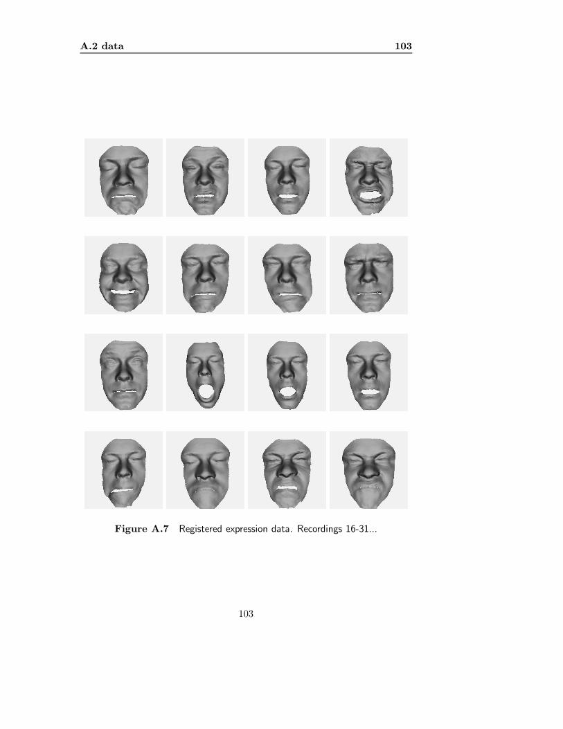
A.2 data 103

Figure A.7 Registered expression data. Recordings 16-31...

103

104 Appendix A

Figure A.8 Registered expression data. Recordings 32:35

104

A.2 data 105

A.2.4 registered ID

Figure A.9 Registered ID data. Recordings 0:16

105

106 Appendix A

Figure A.10 Registered ID data. Recordings 17:23

106

A.3 IMM face database images 107

A.3 IMM face database images

107

108 Appendix A

Figure A.11 Imm face database sample images. Front.

108


Figure A.12 Imm face database sample images. Profile.

109

110 Appendix A

Figure A.13 Imm face database sample images. Smile.

110


Figure A.14 Imm face database sample images. Expression.

111

112 Appendix A

A.4 threedit

files and dependencies

threedit.tar.gz The main octave/matlab package, providing the 3D scenemodelling and rendering rutines, the segmentation and the initializa-tion rutines.

threedit facedata.tar.gz Shape and texture data samples for face mod-elling. Raw and registered. Expression and ID data.

threedit editing programs.tar.gz Editors for texture coordinates, 3D shapeediting and registrator programs.

www.octave.org an open source matlab clone .. lots of extra packages, seeeg. octave.sourceforge.net/packages.html

www.vtk.org (Only needed for the editing programs.) An open sourcevisualization program. C++ programs with Python, Java and Tcl/Tkinterfaces.

www.tcl.tk (Only for the editing programs.) Used for the GUI of theediting software.

A.4.1 Octave rendering and 3D object segmentation software

The main program package, with octave .m files and some .c files.Program contains a lot of comments, and should (is hoped to) be self ex-planatory.

A.4.1.1 .m sample code

ini_ini

ini_system

snapshot

showModelAndSampleOverlay

%% manual model placement

parameters = addRotation (parameters,[0 1 0],20);

parameters = addTranslation(parameters,-0.3,0.2,0);

112

A.4 threedit 113

snapshot


%% construct aaaam .. explore variability in 2d image plane

aaaam.pose.rotX = linspace(-4,4,2);

aaaam.pose.rotY = linspace(-8,8,5);

aaaam.pose.rotZ = linspace(-4,4,2);

aaaam.pose.tX = linspace(-0.1,0.1,4);

aaaam.pose.tY = linspace(-0.1,0.1,4);

aaaam.pose.tZ = linspace(-0.2,0.2,4);

aaaam.modes.id = [-1,1];

aaaam.modes.exp = [];

aaaam.modes.texture = [];

aaaam.light.position = [];

aam.additionalPertParameters = [];

aaaam_run

aam.c = zeros(aam.NCmodes,1);

aam_optimize

snapshot


%% optimize using full 3d-system Jacobian

optimize_initialize

optimize_expression_and_position

%% optimize_all

snapshot


113

114 Appendix A

A.4.2 3D shape editor

Figure A.15 tcl/vtk 3D shape editing tool. Included: add points, deletepoints, delete regions, move points, add triangle, delete trian-gle, smooth surface, simplify surface, split triangles (ie openmesh).

....... xxxxxx ........

--- general ---

’v’: view ... center shape

’s’: surface

’w’: wireframe

’q’: quit

--- landmarks ---

’l’: add a new landmark

’n’: choose nearest landmark

’m’: move choosen landmark to current position

--- edit ---

’a’: add a point to be moved or removed

’t’: add a point marking top corner of ’region’

’b’: add a point marking bottom corner of ’region’

’c’: clear all edit points

’d’: delete current point

’1’: mark triangle vertex 1



....... xxxxxx ........

114

A.4 threedit 115

A.4.3 texture coordinate editor

(a) Points picked on 3D model and in2D image.

(b) Warping applied. Ready for addi-tional fine tuning points.

Figure A.16 tcl/vtk tcoords editor, interactively set points on 3D shape andcorresponding points in image. Thin plate spline warp plus afine tuninig functionality.

....... xxxxxx ........

Texture Mapper

-- add points (IN SAME ORDER) to shape and image --

key ’a’: add point to 3d shape

key ’d’: delete point selected in model viewer

key ’r’: delete ALL points in image

key ’t’: pick point id. translate tcoords with ’z,x,c,v’.

key ’z’: move selected id one pix to the left

key ’x’: right

key ’c’: down

key ’v’: up

key ’left mouse’: add point to 2d image

....... xxxxxx ........

115

116 Appendix A

A.4.4 triangulator

Figure A.17 Manually triangluate a point cloud, good for small surfaces orspecial requests.

....... xxxxxx ........

’a’: pick triangle vertex number 1

’b’: pick triangle vertex number 2

’c’: pick triangle vertex number 3

’p’: view as points

’s’: surface

’w’: wireframe

’t’: add triangle (after points are marked with keys a,b and c)

’d’: delete selected point

(buttons for ’delete triangle’, and ’add triangle’)

....... xxxxxx ........

116

A.4 threedit 117

A.4.5 registrator

Figure A.18 Manually select landmarks on both shapes (or load these) Align(similarity or rigid transform) or warp (thin plate spline). Reg-istrate with closest surface point registration.

--- general ---

’v’: view ... center shape

’s’: surface

’w’: wireframe

’q’: quit

--- landmarks ---

’l’: add a new landmark

’n’: choose nearest landmark

’m’: move choosen landmark to current pointer position

--- edit ---

’a’: add a point to be moved or removed

’t’: add a point marking top corner of ’region’

’b’: add a point marking bottom corner of ’region’

’c’: clear all edit points

’d’: delete current point




--- stuff ---

regA2B: ... copy closest surface point on B to A structure ...

117

Documents

preface - · PDF filepreface The work presented in this thesis has ... project. The work done on face ... proach this goal by investigating statistical diﬀerences in two sets of