Embed Size (px)
Citation preview
Preface This thesis is submitted for partial fulfillment of the requirements for the degree of Doctor of Philosophy in Energy Engineering at Aalborg University. The work has been carried out in the period Mars 2003 to June 2007 and is part of the PSO2002-4730 project: Development of generalized model for grate combustion of biomass. Firstly, I would like to acknowledge my supervisors, Associate Professor Lasse Rosendahl and Associate Professor Søren Knudsen Kær, as well as my colleges at the institute of Energy Technology at Aalborg University. Special thanks to Henrik Sørensen for valuable input and help to the experimental work. I would also like to thank Jan Christiansen and Mads Lund for all their support in the workshop. Furthermore, I would like to thank Rasmus Jensen and Melissa Berry, whose student projects have contributed with important experimental data to this thesis. Part of this work was carried out during a five months long stay at Sheffield University Waste Incineration Centre (SUWIC), UK. I would like to thank Professor Jim Swithenbank, Professor Vida N Sharifi and Dr. Yao-bin Yang for excellent guidance and valuable discussions. I would also like to thank the other PhD students at SUWIC, who all made my stay in Sheffield very pleasant and memorable. Finally, I would like to thank my family and friends for always being there and supporting me. I am so grateful for having such wonderful friends. A special thank you to Jenny and Søren, for their great hospitality and making Aalborg feel like home. Without you I would never have made it all the way. Hanna Sabelström Aalborg, June 2007

Abstract This work is part of a long term project of developing a bed model, describing the combustion process of straw on a vibrating grate. For a vibrating grate, the mixing and transportation of the fuel are of great significance and the work presented in this report investigates how the effect of vibrations can be incorporated into a numerical model.
The chosen model approach has been to separate the gas and solid phases into two independent models related to each other through the bed porosity. By treating the bed as a porous media and using Ergun’s equation for the gas flow, the numerical work is simplified and the computational time shortened. The vibrations are affecting the transport and mixing of the fuel and incorporated into the model through the diffusion coefficient in the conservation equation of the solid phase.
Experimental work has been carried out with the aim to study the behaviour of wood pellets on a vibrating grate and deriving the diffusion coefficient to be used in the numerical model. Three different grate designs are used and the particle trajectories have been captured by a camera placed above the grate. The diffusion coefficient is defined as the deviation from the mean movement of the particles. The results show that the diffusion of the particles increases with increasing vibration amplitude and frequency and decreasing particle layer thickness. There is a significant difference in the magnitude of the diffusion coefficients for the different test set-ups, which shows that the diffusion is strongly dependent on the grate design and a diffusion coefficient has to be determined for each type of grate to be modeled.
Different alternatives of how to represent the velocity and diffusion coefficients in the model have been investigated. It has been found that the vibrations give rise to both a diffusive and a convective contribution and that the velocity depends on the position of the grate. It is suggested that the mean velocity of the particles should be seen as a convective process whilst the deviation from the mean velocity should be treated as a diffusive process. In order to introduce a varying velocity depending on the position on the grate, a modification of the model is necessary where also the density will vary as a consequence of the continuity equation. The definition of the density will thereby change from being the particle density to be the cell density, i.e. a measure of how dense the particles are packed in each cell.

Contents
i
Contents 1 Introduction
1.1 Climate Changes ……………………………………………............
1.2 Biomass as renewable energy source ………………………………
1.3 The use of CFD for designing and optimising furnaces ……………
1.4 Problem statement ………………………………………………….
1.5 Report structure ………………………………………………….…
2 Biomass- an overview
2.1 Biomass properties ……………………………………………….…
2.2 Fuel characterisation ……………………………………………..…
2.2.1 Wood …………………………………………………….…
2.2.2 Herbaceous and annual growth materials- straw …………...
2.2.3 Agricultural wastes and residues …………………………...
2.2.4 Refused-derived fuels and combustible waste ……………..
2.3 Chemical composition of biomass ………………………………….
2.4 Thermal conversion ………………………………………………...
2.5 Combustion technologies …………………………………………...
2.5.1 Fluidised bed combustion …………………………………..
2.5.2 Fixed bed combustion- grate furnaces ……………………...
2.5.3 Travelling grate and moving grate ……………………….....
2.5.4 Vibrating grate ……………………………………………...
2.5.5 Suspension firing …………………………………………...
2.6 Emissions …………………………………………………………...
1
1
1
2
3
4
5
6
7
7
7
8
8
8
9
11
11
12
13
14
14
14
Diffusion of solid fuel on a vibrating grate
ii
3 Bed models- state of the art
3.1 Kinetics …………………………………………………………..…
3.2 Modelling of a single particle ………………………………………
3.3 Modelling of fixed and moving beds ………………………………
3.3.1 Ignition front ………………………………………….……
3.3.2 Primary air flow ………………………………………….…
3.4 Bed models …………………………………………………………
4 Mixing theory of particles
4.1 Gas kinetic theory ……………………………………………..……
4.2 Maxwell-Boltzmann distribution function …………………………
4.3 Brownian motion …………………………………………………...
4.4 Diffusion ……………………………………………………………
4.4.1 Transport equation ……………………………………………
4.5 Particle mixing ……………………………………………………...
4.6 Granular flow ………………………………………………….……
4.7 Simulation of granular material ……………………………….……
4.7.1 Continuum mechanics approach ……………………………
4.7.2 Discrete element approach …………………………………
4.7.3 Event Driven Method- hard sphere method ………..………
4.7.4 Time Driven Method- soft particle method ………………...
4.7.5 Kinetic theory approach ………………………………….…
4.8 Vibration of granular material ……………………………………...
4.9 Mixing in bed models ………………………………………………
4.10 Mixing process on a vibrating grate …………………………..……
4.11 Diffusion concept of this project …………………………………...
5 Experimental work
5.1 Rig constructions / vibrating grate systems ………………………...
5.1.1 Grate A- pneumatically driven vibrations ………….………
5.1.2 Grate B- vibrations induced by amplitude wheel …………..
5.1.3 Grate C- pivoting grate ………………………………..……
5.2 Particle types ……………………………………………………..…
17
18
19
21
21
22
23
31
32
32
33
33
33
34
34
36
37
37
37
38
39
41
44
45
46
49
50
50
52
53
55
Contents
iii
5.3 Data treatment ………………………………………………………
5.4 Experiments on grate A ………………………………….…………
5.5 Experiments on grate B …………………………………….………
5.6 Experiments on grate C …………………………………….………
5.7 Results and discussion ……………………………………………...
5.7.1 Results- grate A ……………………………………….……
5.7.2 Results- grate B …………………………………………..…
5.7.3 Grate B- variation of Dx along the grate ……………………
5.7.4 Grate B- variation of Dx across the grate …………………...
5.7.5 Grate B- comparison of Dx and Dy ………………….………
5.7.6 Grate B- influence of frequency and amplitude ……………
5.7.7 Grate B- Influence of grate construction …………………...
5.7.8 Results- grate C …………………………………….….……
5.7.9 Grate C- variation of Dx and Dy along the grate ……………
5.7.10 Grate C- variation of Dx and Dy aross the grate ……………
5.7.11 Grate C- dependency on frequency …………...……………
5.7.12 Grate C- influence of grate construction …………………...
5.8 Comparison between the experiments ……………………………...
5.9 Comparison to literature ……………………………………………
5.9.1 Comparison with theoretical diffusion coefficient …………
5.9.2 Comparison to experiments by Yang et al. …………………
5.10 Experiences from an industrial vibrating grate …………………..…
5.11 Future investigations ……………………………………………..…
5.12 Conclusion / summary …………………………………………...…
6 Modelling work
6.1 Model structure …………………………………………………….
6.2 Gas phase ………………………………………………………...…
6.2.1 Porosity ……………………………………………………..
6.2.2 Test of Ergun’s equation ……………………………………
6.3 Solid phase …………………………………………………….……
6.4 The Finite Volume Method ………………………………...………
6.5 Test cases ……………………………………………………...……
56
57
59
60
62
62
64
64
65
66
67
69
70
71
73
75
77
79
80
81
83
84
85
86
87
88
89
90
90
92
94
95
Diffusion of solid fuel on a vibrating grate
iv
6.5.1 Test case 1- constant velocity and diffusion coefficient ……
6.5.2 Test case 2- varying diffusion coefficient ……….…………
6.5.3 Test case 3- Varying velocity ………………………………
6.5.4 Test case 4- Comparison to a real case …………..…………
6.6 Future work …………………………………………………………
6.6.1 Three dimensions ………………………………………...…
6.6.2 Combustion …………………………………………………
7 Conclusion and perspectives
8 References
Appendix A
97
101
102
103
108
108
108
109
113
119
Chapter1: Introduction
1
1 Introduction 1.1 Climate changes At the moment a rapidly growing interest and concern about climate changes is taking place globally. A contributing factor to the growing interest is the increasing number of extreme weather events all over the world with catastrophic consequences for millions of people. Some examples are high frequency of heavy precipitation, longer and more severe droughts, an increase of intense tropical cyclone activities, increasing number of heat waves and decreasing snow cover. Most researchers have agreed that these climate changes are caused by high concentrations of greenhouse gases produced by mankind, resulting in an increased average temperature of the atmosphere. An important greenhouse gas is CO2, emitted as a consequence of combustion of fossil fuel such as coal and oil. The CO2 emissions have grown from 1970 to 2004 by about 80% (IPCC, 2007). To change the trend of an increasing average global temperature, drastic actions need to be undertaken concerning emissions in general and of CO2 in particular. The western society today is highly energy consuming and there is a fast going development taking place in the east and in developing countries pointing towards an even higher energy demand in the future. It is therefore extremely important to find and start using new, sustainable energy sources to replace the fossil fuel. Strong political actions have started to take form, the well known Kyoto agreement is one example where countries have obliged to reduce their emissions of greenhouse gases with 5.2% by year 2012, based on year 1990 levels. The political actions also lead to an increased interest and amount of research activities within renewable energy resources like wind, solar, wave and biomass.
1.2 Biomass as renewable energy source To replace fossil fuel by biomass is one step to achieve a reduction of the CO2 emissions to the atmosphere. Biomass is considered to be CO2 neutral since it is fast growing and thereby consuming an equal amount of CO2 as produced during combustion, provided that re-plantation is done. Biomass is a very heterogeneous group of fuel, comprising wood, bark, branches, twigs, various kinds of crops, straw, olive stones, rape-oil, ethanol and many other things. Today, biomass contributes to approximately 14% of the world’s total energy supply (Yang et al., 2005a). However, this number also includes primitive combustion methods, without any process control or emission reductions, that are frequently used in the third world. In Denmark, which is a country with a lot of cultivated land and not so many forests, straw is a commonly used biomass fuel. Straw is a very complex fuel, containing high levels of
Diffusion of solid fuel on a vibrating grate
2
potassium, chlorine and sulphur, causing severe corrosion problems in the combustion chamber. There are also large problems in the form of formation of deposits and slagging on the heat transfer surfaces in the furnace, leading to decreased furnace efficiency. When burning straw to generate heat and energy it can be used on its own or in co-combustion with coal or wood. When used on it its own straw is generally burnt on a vibrating grate. Vibrating grates have shown to be a well suited method for straw combustion, since the vibrations tend to prevent agglomeration of the straw. However, an additional problem during combustion of straw on vibrating grates is the high occurrence of emissions peaks, most likely related to the vibration movements. Even though biomass is the oldest type of fuel for small scale, domestic energy production, modern, large scale biomass combustion is still a fairly new technology. The fuel properties of biomass differ from those of traditional fuels like coal and oil and to achieve an effective combustion with a minimum of emissions, modifications of existing technology are necessary.
1.3 The use of CFD for designing and optimising furnaces When designing grates and furnaces the applied technology is based on experience and not much on theoretical studies. By developing numerical methods of the process in the furnace a detailed knowledge can be achieved and valuable insights can be drawn. By simulating the combustion behaviour, different parameters can be studied such as fuel type, fuel properties and air distribution and their effect on the emission levels and furnace efficiency, without having to make expensive and time consuming real scale measurements, Computational Fluid Dynamics (CFD) has become an increasingly used tool for this type of calculations. Lots of research work is carried out in developing CFD models of the free board area in the furnace to investigate the optimal air distribution and identify recirculation zones. A frequent problem with the CFD codes is that there is a lack of accurate inlet conditions from the fuel bed. The process in the fuel bed is of great significance and it would be extremely valuable to be able to predict the right distribution and amount of particles and volatiles leaving the bed to use as inlet conditions to a CFD model. The purpose of bed models is not uniquely to provide inlet conditions to CFD models, it is also of great importance to study the combustion process inside the bed and understanding the underlying mechanisms. Bed models have been developed for different types of grates, such as fixed beds and travelling grates, and many kinds of biomass fuels, e.g. wood, wood chips, waste and saw dust. So far, only limited research work has been carried out for vibrating grates. Focus within bed modelling has mainly been on the chemical conversion of biomass and not so much on the mass transport mechanisms. However, for a vibrating grate, the moving mechanisms are of high importance and do play a significant part for the mixing and combustion process in the fuel bed. If, for example, the highly frequent occurring emission peaks could be captured by mathematical modelling, it would be a revolutionary contribution to the work of preventing such peaks and thereby achieving a more optimal combustion.
Chapter1: Introduction
3
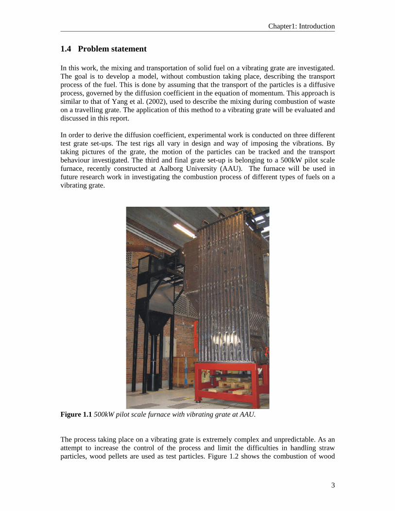
1.4 Problem statement In this work, the mixing and transportation of solid fuel on a vibrating grate are investigated. The goal is to develop a model, without combustion taking place, describing the transport process of the fuel. This is done by assuming that the transport of the particles is a diffusive process, governed by the diffusion coefficient in the equation of momentum. This approach is similar to that of Yang et al. (2002), used to describe the mixing during combustion of waste on a travelling grate. The application of this method to a vibrating grate will be evaluated and discussed in this report. In order to derive the diffusion coefficient, experimental work is conducted on three different test grate set-ups. The test rigs all vary in design and way of imposing the vibrations. By taking pictures of the grate, the motion of the particles can be tracked and the transport behaviour investigated. The third and final grate set-up is belonging to a 500kW pilot scale furnace, recently constructed at Aalborg University (AAU). The furnace will be used in future research work in investigating the combustion process of different types of fuels on a vibrating grate.
Figure 1.1 500kW pilot scale furnace with vibrating grate at AAU. The process taking place on a vibrating grate is extremely complex and unpredictable. As an attempt to increase the control of the process and limit the difficulties in handling straw particles, wood pellets are used as test particles. Figure 1.2 shows the combustion of wood
Diffusion of solid fuel on a vibrating grate
4
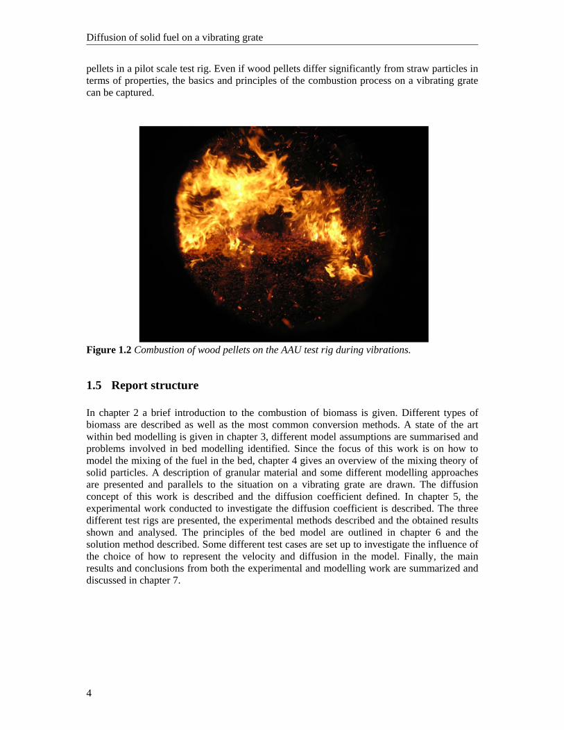
pellets in a pilot scale test rig. Even if wood pellets differ significantly from straw particles in terms of properties, the basics and principles of the combustion process on a vibrating grate can be captured.
Figure 1.2 Combustion of wood pellets on the AAU test rig during vibrations.
1.5 Report structure In chapter 2 a brief introduction to the combustion of biomass is given. Different types of biomass are described as well as the most common conversion methods. A state of the art within bed modelling is given in chapter 3, different model assumptions are summarised and problems involved in bed modelling identified. Since the focus of this work is on how to model the mixing of the fuel in the bed, chapter 4 gives an overview of the mixing theory of solid particles. A description of granular material and some different modelling approaches are presented and parallels to the situation on a vibrating grate are drawn. The diffusion concept of this work is described and the diffusion coefficient defined. In chapter 5, the experimental work conducted to investigate the diffusion coefficient is described. The three different test rigs are presented, the experimental methods described and the obtained results shown and analysed. The principles of the bed model are outlined in chapter 6 and the solution method described. Some different test cases are set up to investigate the influence of the choice of how to represent the velocity and diffusion in the model. Finally, the main results and conclusions from both the experimental and modelling work are summarized and discussed in chapter 7.
Chapter 2: Biomass- an overview
5
2 Biomass- an overview
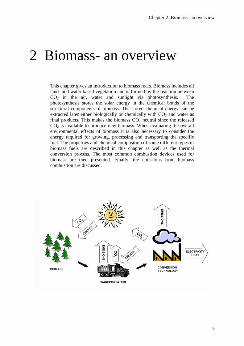
This chapter gives an introduction to biomass fuels. Biomass includes all land- and water based vegetation and is formed by the reaction between CO2 in the air, water and sunlight via photosynthesis. The photosynthesis stores the solar energy in the chemical bonds of the structural components of biomass. The stored chemical energy can be extracted later either biologically or chemically with CO2 and water as final products. This makes the biomass CO2 neutral since the released CO2 is available to produce new biomass. When evaluating the overall environmental effects of biomass it is also necessary to consider the energy required for growing, processing and transporting the specific fuel. The properties and chemical composition of some different types of biomass fuels are described in this chapter as well as the thermal conversion process. The most common combustion devices used for biomass are then presented. Finally, the emissions from biomass combustion are discussed.
Diffusion of solid fuel on a vibrating grate
6
2.1 Biomass Properties There is a wide range of biomass fuel and the composition and properties are varying depending on species, type of plant tissue, growing stage and growing conditions. Despite the many differences in composition and properties the energy content of biomass (on ash free dry basis) is similar for all plant species, lying in the range of 17-21 MJ/kg (McKendry, 2002). The fuel properties influence the rate of combustion as well as the efficiency of the combustion system. It is important to identify the properties of the fuel and to make sure that the chosen operational way is suited for that specific fuel. Important physical and chemical parameters are:
• Particle dimensions • Bulk density • Calorific value • Moisture content • Proportions of fixed carbon and volatiles • Ash/residue content • Alkali metal content • Cellulose/lignin ratio
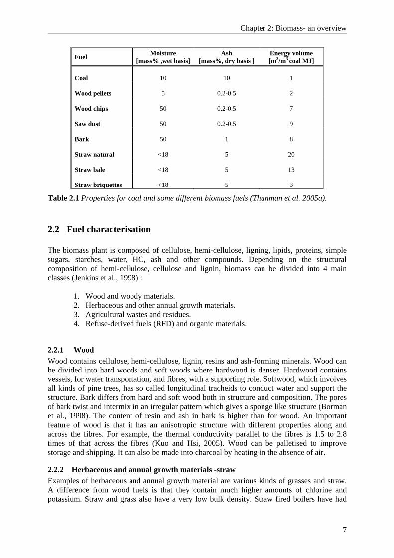
The knowledge of these parameters is needed to be able to adjust the temperature control system of the furnace and to design the volume and geometry of the furnace to achieve an efficient combustion. Particle diameters can vary from a few millimetres to about 50 cm and the size distribution can be homogeneous (e.g. pellets) or inhomogeneous (e.g. wood chips). The particle dimension and size distribution are important parameters when choosing appropriate fuel feeding system and combustion technology. The bulk density and calorific value influence the fuel logistics such as transport and storage as well as the process control of the fuel feeding system. The moisture content of the fuel influences the combustion behaviour, the adiabatic temperature of combustion and the volume of flue gas produced per energy unit. Fuel with a high moisture content needs a longer residence time to dry before the volatile release and char combustion takes place, which requires a bigger combustion chamber. Combustion is only feasible for biomass with a moisture content less than 50% (McKendry, 2002). Biomass fuel with higher moisture content is better suited to biological conversion processes such as fermentation. Moisture, ash and energy volume for coal and some different types of biomass are shown in Table 2.1 The energy volume is important when considering the transportation method and, in this case, is related to the energy content of 1m3 of coal. It can be seen that for natural straw 20 times the volume of coal is required to achieve the same energy output while for straw briquettes the number has decreased to 3.
Chapter 2: Biomass- an overview
7
Fuel Moisture [mass% ,wet basis]
Ash [mass%, dry basis ]
Energy volume [m3/m3 coal MJ]
Coal 10 10 1 Wood pellets 5 0.2-0.5 2 Wood chips 50 0.2-0.5 7 Saw dust 50 0.2-0.5 9 Bark 50 1 8 Straw natural <18 5 20 Straw bale <18 5 13 Straw briquettes <18 5 3
Table 2.1 Properties for coal and some different biomass fuels (Thunman et al. 2005a).
2.2 Fuel characterisation The biomass plant is composed of cellulose, hemi-cellulose, ligning, lipids, proteins, simple sugars, starches, water, HC, ash and other compounds. Depending on the structural composition of hemi-cellulose, cellulose and lignin, biomass can be divided into 4 main classes (Jenkins et al., 1998) :
1. Wood and woody materials. 2. Herbaceous and other annual growth materials. 3. Agricultural wastes and residues. 4. Refuse-derived fuels (RFD) and organic materials.
2.2.1 Wood Wood contains cellulose, hemi-cellulose, lignin, resins and ash-forming minerals. Wood can be divided into hard woods and soft woods where hardwood is denser. Hardwood contains vessels, for water transportation, and fibres, with a supporting role. Softwood, which involves all kinds of pine trees, has so called longitudinal tracheids to conduct water and support the structure. Bark differs from hard and soft wood both in structure and composition. The pores of bark twist and intermix in an irregular pattern which gives a sponge like structure (Borman et al., 1998). The content of resin and ash in bark is higher than for wood. An important feature of wood is that it has an anisotropic structure with different properties along and across the fibres. For example, the thermal conductivity parallel to the fibres is 1.5 to 2.8 times of that across the fibres (Kuo and Hsi, 2005). Wood can be palletised to improve storage and shipping. It can also be made into charcoal by heating in the absence of air.
2.2.2 Herbaceous and annual growth materials -straw Examples of herbaceous and annual growth material are various kinds of grasses and straw. A difference from wood fuels is that they contain much higher amounts of chlorine and potassium. Straw and grass also have a very low bulk density. Straw fired boilers have had
Diffusion of solid fuel on a vibrating grate
8
major operational problems because of rapid deposit accumulation and corrosion rates. An advanced logistic system and proper combustion technology are fundamental requirements when straw combustion is considered. The lowest levels of slagging fouling and corrosion have been achieved with pulverised combustion (Veijonen et al., 2003). If straw is left on the fields during a period before harvesting and thereby “washed” by rain, the contents of chlorine and potassium will be lower. Attempts have also been made washing the straw in 50-60˚C before introducing it into the furnace. The energy loss when washing and drying the straw is estimated to be about 8% of the heating value (Nikolaisen et al., 1998). The costs of the washing procedure, however, must be compared to the savings due to a longer life time of the combustion equipment. The growing climate is important as it influences the moisture content of the straw. Time of the year of harvesting, and the type of soil where it is growing, are also important factors to consider for annual fuel crops.
2.2.3 Agricultural wastes and residues Agriculture wastes comprise crop residues as well as manure. Crop residues are the plant parts that are left after the harvesting, such like nut husks and olive pits. Since agricultural wastes and residues differ significantly in structure and content it is important to distinguish the different types so that an appropriate conversion technique can be chosen. Manure is a high moisture material and therefore more suited for “wet” processing techniques such as fermentation or other biologically conversion methods.
2.2.4 Refused-derived fuels and combustible waste Burning of waste materials has increased in recent times, in the effort in using more renewable energy sources. Another drive for burning waste is the lack of land and global regulations against land filling which used to be the most common waste treatment. Waste can be burned directly in dedicated boilers or it can processed first and divided into combustibles and non-combustibles. The processing includes shredding, magnetic separation, screening and air classification with the purpose of recovering glass and metal and to reduce the fuel size. Processed fuel is called Refuse Derived Fuel (RDF) and can also be compressed into pellets or briquettes for better storing and shipping or thermally converted to liquid and gaseous fuels.
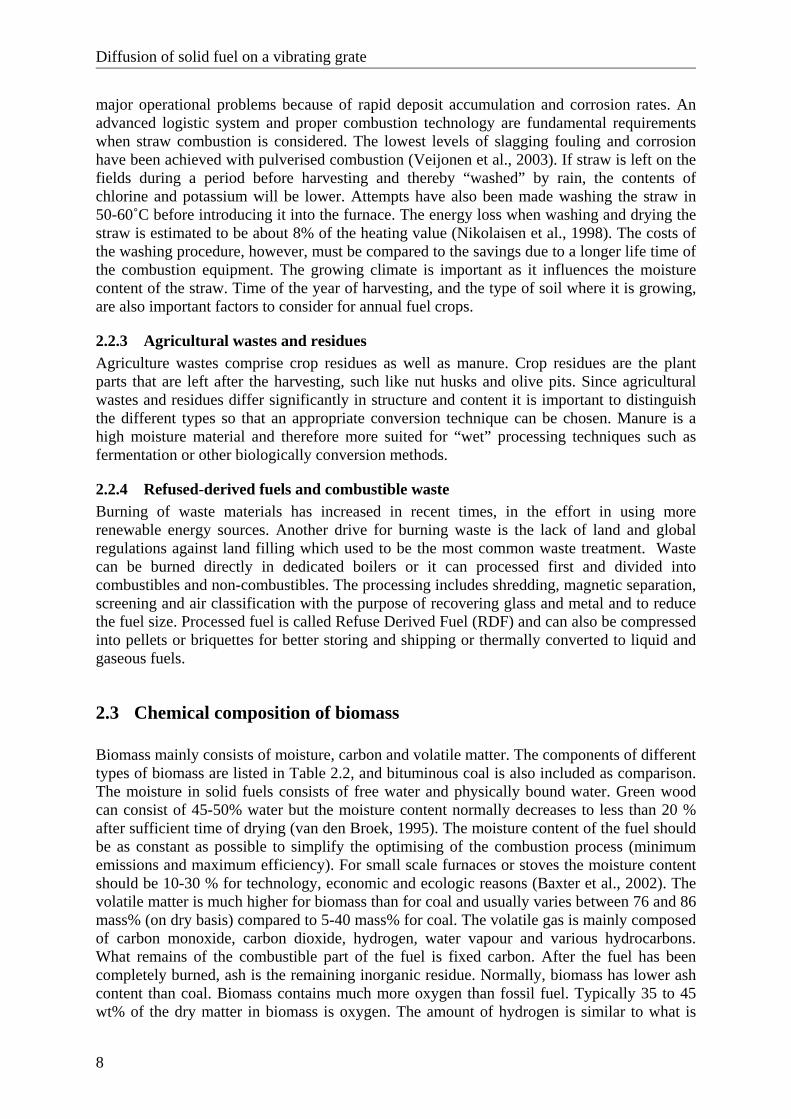
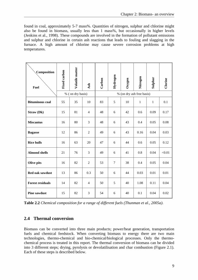
2.3 Chemical composition of biomass Biomass mainly consists of moisture, carbon and volatile matter. The components of different types of biomass are listed in Table 2.2, and bituminous coal is also included as comparison. The moisture in solid fuels consists of free water and physically bound water. Green wood can consist of 45-50% water but the moisture content normally decreases to less than 20 % after sufficient time of drying (van den Broek, 1995). The moisture content of the fuel should be as constant as possible to simplify the optimising of the combustion process (minimum emissions and maximum efficiency). For small scale furnaces or stoves the moisture content should be 10-30 % for technology, economic and ecologic reasons (Baxter et al., 2002). The volatile matter is much higher for biomass than for coal and usually varies between 76 and 86 mass% (on dry basis) compared to 5-40 mass% for coal. The volatile gas is mainly composed of carbon monoxide, carbon dioxide, hydrogen, water vapour and various hydrocarbons. What remains of the combustible part of the fuel is fixed carbon. After the fuel has been completely burned, ash is the remaining inorganic residue. Normally, biomass has lower ash content than coal. Biomass contains much more oxygen than fossil fuel. Typically 35 to 45 wt% of the dry matter in biomass is oxygen. The amount of hydrogen is similar to what is
Chapter 2: Biomass- an overview
9
found in coal, approximately 5-7 mass%. Quantities of nitrogen, sulphur and chlorine might also be found in biomass, usually less than 1 mass%, but occasionally in higher levels (Jenkins et al., 1998). These compounds are involved in the formation of pollutant emissions and sulphur and chlorine in certain ash reactions that leads to fouling and slagging in the furnace. A high amount of chlorine may cause severe corrosion problems at high temperatures.
Fixe
d ca
rbon
Vol
atile
mat
ter
Ash
Car
bon
Hyd
roge
n
Oxy
gen
Nitr
ogen
Sulp
hur
Clo
rine
Composition Fuel
% ( on dry basis) % (on dry ash free basis) Bituminous coal
55 35 10 83 5 10 1 1 0.1
Straw (Dk)
15 81 4 48 6 42 0.6 0.09 0.17
Miscantus
16 80 3 48 6 43 0.4 0.05 0.08
Bagasse
12 86 2 49 6 43 0.16 0.04 0.03
Rice hulls
16 63 20 47 6 44 0.6 0.05 0.12
Almond shells
21 76 3 49 6 41 0.8 0.04 <0.01
Olive pits
16 82 2 53 7 38 0.4 0.05 0.04
Red oak sawdust
13 86 0.3 50 6 44 0.03 0.01 0.01
Forest residuals
14 82 4 50 5 40 1.08 0.11 0.04
Pine sawdust
15 82 3 54 6 40 0.1 0.04 0.02
Table 2.2 Chemical composition for a range of different fuels (Thunman et al., 2005a).
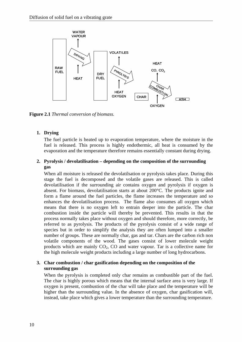
2.4 Thermal conversion Biomass can be converted into three main products; power/heat generation, transportation fuels and chemical feedstock. When converting biomass to energy there are two main technologies, thermo-chemical and bio-chemical/biological processes. Only the thermo-chemical process is treated in this report. The thermal conversion of biomass can be divided into 3 different steps; drying, pyrolysis or devolatilisation and char combustion (Figure 2.1). Each of these steps is described below.
Diffusion of solid fuel on a vibrating grate
10
RAW FUEL
DRYFUEL
CHARASH
PYROLYSIS
DRYING
CHAR COMBUSTION
HEAT
WATER VAPOUR
HEAT
HEAT
OXYGEN
VOLATILES
OXYGEN
CO, CO2
RAW FUEL
DRYFUEL
CHARASH
PYROLYSIS
DRYING
CHAR COMBUSTION
HEAT
WATER VAPOUR
HEAT
HEAT
OXYGEN
VOLATILES
OXYGEN
CO, CO2
Figure 2.1 Thermal conversion of biomass.
1. Drying The fuel particle is heated up to evaporation temperature, where the moisture in the fuel is released. This process is highly endothermic, all heat is consumed by the evaporation and the temperature therefore remains essentially constant during drying.
2. Pyrolysis / devolatilisation – depending on the composition of the surrounding gas When all moisture is released the devolatilsation or pyrolysis takes place. During this stage the fuel is decomposed and the volatile gases are released. This is called devolatilisation if the surrounding air contains oxygen and pyrolysis if oxygen is absent. For biomass, devolatilisation starts at about 200°C. The products ignite and form a flame around the fuel particles, the flame increases the temperature and so enhances the devolatilisation process. The flame also consumes all oxygen which means that there is no oxygen left to entrain deeper into the particle. The char combustion inside the particle will thereby be prevented. This results in that the process normally takes place without oxygen and should therefore, more correctly, be referred to as pyrolysis. The products of the pyrolysis consist of a wide range of species but in order to simplify the analysis they are often lumped into a smaller number of groups. These are normally char, gas and tar. Chars are the carbon rich non volatile components of the wood. The gases consist of lower molecule weight products which are mainly CO2, CO and water vapour. Tar is a collective name for the high molecule weight products including a large number of long hydrocarbons.
3. Char combustion / char gasification depending on the composition of the surrounding gas When the pyrolysis is completed only char remains as combustible part of the fuel. The char is highly porous which means that the internal surface area is very large. If oxygen is present, combustion of the char will take place and the temperature will be higher than the surrounding value. In the absence of oxygen, char gasification will, instead, take place which gives a lower temperature than the surrounding temperature.
Chapter 2: Biomass- an overview
11
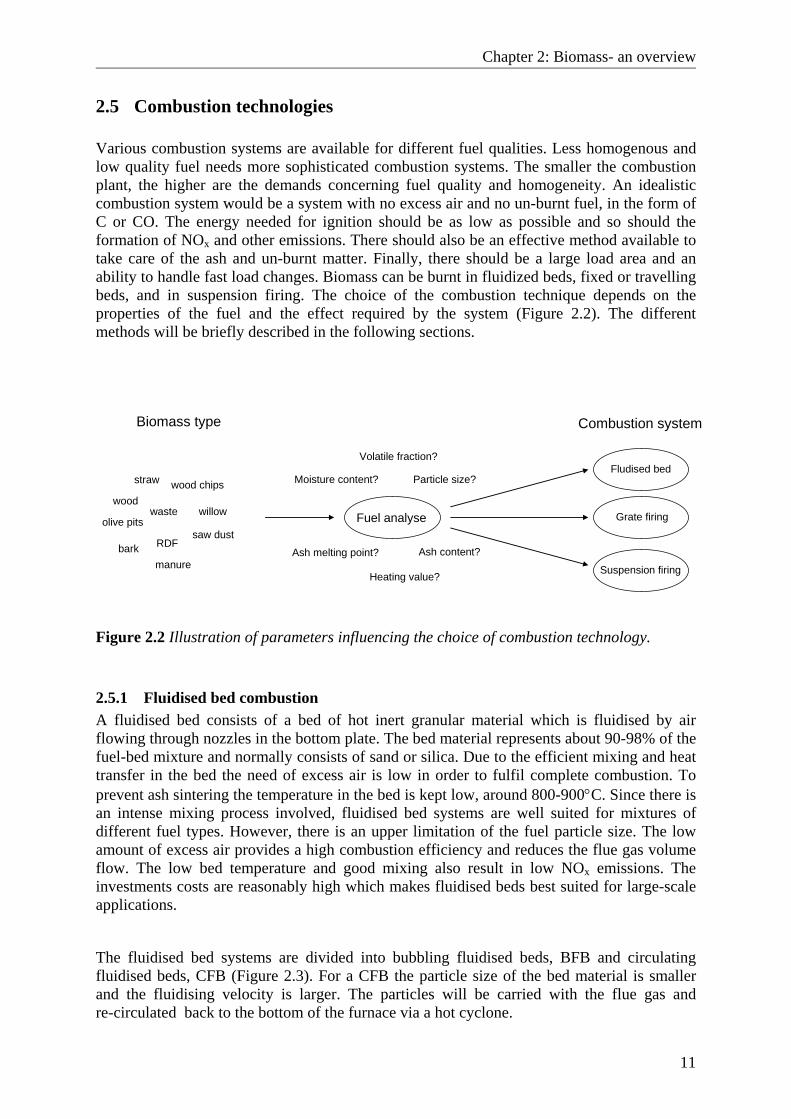
2.5 Combustion technologies Various combustion systems are available for different fuel qualities. Less homogenous and low quality fuel needs more sophisticated combustion systems. The smaller the combustion plant, the higher are the demands concerning fuel quality and homogeneity. An idealistic combustion system would be a system with no excess air and no un-burnt fuel, in the form of C or CO. The energy needed for ignition should be as low as possible and so should the formation of NOx and other emissions. There should also be an effective method available to take care of the ash and un-burnt matter. Finally, there should be a large load area and an ability to handle fast load changes. Biomass can be burnt in fluidized beds, fixed or travelling beds, and in suspension firing. The choice of the combustion technique depends on the properties of the fuel and the effect required by the system (Figure 2.2). The different methods will be briefly described in the following sections.
Biomass type Combustion system
Fludised bed
Grate firing
Suspension firing
Fuel analyse
Particle size?
Ash content?
Heating value?
Volatile fraction?
Ash melting point?
Moisture content?straw
wood
olive pitswaste
bark
willow
saw dust
wood chips
manure
RDF
Figure 2.2 Illustration of parameters influencing the choice of combustion technology.
2.5.1 Fluidised bed combustion A fluidised bed consists of a bed of hot inert granular material which is fluidised by air flowing through nozzles in the bottom plate. The bed material represents about 90-98% of the fuel-bed mixture and normally consists of sand or silica. Due to the efficient mixing and heat transfer in the bed the need of excess air is low in order to fulfil complete combustion. To prevent ash sintering the temperature in the bed is kept low, around 800-900°C. Since there is an intense mixing process involved, fluidised bed systems are well suited for mixtures of different fuel types. However, there is an upper limitation of the fuel particle size. The low amount of excess air provides a high combustion efficiency and reduces the flue gas volume flow. The low bed temperature and good mixing also result in low NOx emissions. The investments costs are reasonably high which makes fluidised beds best suited for large-scale applications.
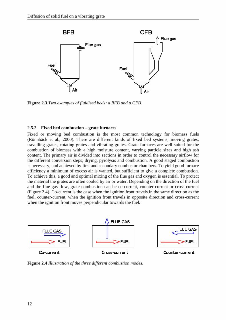
The fluidised bed systems are divided into bubbling fluidised beds, BFB and circulating fluidised beds, CFB (Figure 2.3). For a CFB the particle size of the bed material is smaller and the fluidising velocity is larger. The particles will be carried with the flue gas and re-circulated back to the bottom of the furnace via a hot cyclone.
Diffusion of solid fuel on a vibrating grate
12
Figure 2.3 Two examples of fluidised beds; a BFB and a CFB.
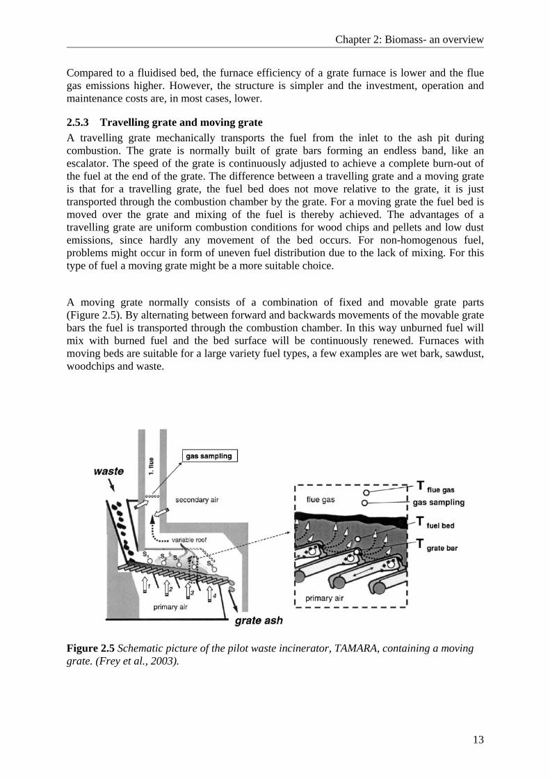
2.5.2 Fixed bed combustion – grate furnaces Fixed or moving bed combustion is the most common technology for biomass fuels (Rönnbäck et al., 2000). There are different kinds of fixed bed systems; moving grates, travelling grates, rotating grates and vibrating grates. Grate furnaces are well suited for the combustion of biomass with a high moisture content, varying particle sizes and high ash content. The primary air is divided into sections in order to control the necessary airflow for the different conversion steps; drying, pyrolysis and combustion. A good staged combustion is necessary, and achieved by first and secondary combustor chambers. To yield good furnace efficiency a minimum of excess air is wanted, but sufficient to give a complete combustion. To achieve this, a good and optimal mixing of the flue gas and oxygen is essential. To protect the material the grates are often cooled by air or water. Depending on the direction of the fuel and the flue gas flow, grate combustion can be co-current, counter-current or cross-current (Figure 2.4). Co-current is the case when the ignition front travels in the same direction as the fuel, counter-current, when the ignition front travels in opposite direction and cross-current when the ignition front moves perpendicular towards the fuel.
Figure 2.4 Illustration of the three different combustion modes.
Chapter 2: Biomass- an overview
13
Compared to a fluidised bed, the furnace efficiency of a grate furnace is lower and the flue gas emissions higher. However, the structure is simpler and the investment, operation and maintenance costs are, in most cases, lower.
2.5.3 Travelling grate and moving grate A travelling grate mechanically transports the fuel from the inlet to the ash pit during combustion. The grate is normally built of grate bars forming an endless band, like an escalator. The speed of the grate is continuously adjusted to achieve a complete burn-out of the fuel at the end of the grate. The difference between a travelling grate and a moving grate is that for a travelling grate, the fuel bed does not move relative to the grate, it is just transported through the combustion chamber by the grate. For a moving grate the fuel bed is moved over the grate and mixing of the fuel is thereby achieved. The advantages of a travelling grate are uniform combustion conditions for wood chips and pellets and low dust emissions, since hardly any movement of the bed occurs. For non-homogenous fuel, problems might occur in form of uneven fuel distribution due to the lack of mixing. For this type of fuel a moving grate might be a more suitable choice.
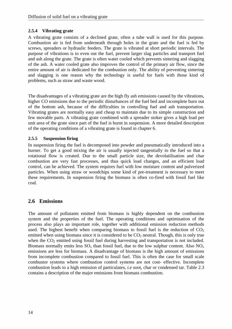
A moving grate normally consists of a combination of fixed and movable grate parts (Figure 2.5). By alternating between forward and backwards movements of the movable grate bars the fuel is transported through the combustion chamber. In this way unburned fuel will mix with burned fuel and the bed surface will be continuously renewed. Furnaces with moving beds are suitable for a large variety fuel types, a few examples are wet bark, sawdust, woodchips and waste.
Figure 2.5 Schematic picture of the pilot waste incinerator, TAMARA, containing a moving grate. (Frey et al., 2003).
Diffusion of solid fuel on a vibrating grate
14
2.5.4 Vibrating grate A vibrating grate consists of a declined grate, often a tube wall is used for this purpose. Combustion air is fed from underneath through holes in the grate and the fuel is fed by screws, spreaders or hydraulic feeders. The grate is vibrated at short periodic intervals. The purpose of vibrations is to even out the fuel, prevent larger slag particles and transport fuel and ash along the grate. The grate is often water cooled which prevents sintering and slagging of the ash. A water cooled grate also improves the control of the primary air flow, since the entire amount of air is dedicated for the combustion only. The ability of preventing sintering and slagging is one reason why the technology is useful for fuels with those kind of problems, such as straw and waste wood.
The disadvantages of a vibrating grate are the high fly ash emissions caused by the vibrations, higher CO emissions due to the periodic disturbances of the fuel bed and incomplete burn out of the bottom ash, because of the difficulties in controlling fuel and ash transportation. Vibrating grates are normally easy and cheap to maintain due to its simple construction and few movable parts. A vibrating grate combined with a spreader stoker gives a high load per unit area of the grate since part of the fuel is burnt in suspension. A more detailed description of the operating conditions of a vibrating grate is found in chapter 6.
2.5.5 Suspension firing In suspension firing the fuel is decomposed into powder and pneumatically introduced into a burner. To get a good mixing the air is usually injected tangentially to the fuel so that a rotational flow is created. Due to the small particle size, the devolatilisation and char combustion are very fast processes, and thus quick load changes, and an efficient load control, can be achieved. The system requires fuel with low moisture content and pulverized particles. When using straw or woodchips some kind of pre-treatment is necessary to meet these requirements. In suspension firing the biomass is often co-fired with fossil fuel like coal.
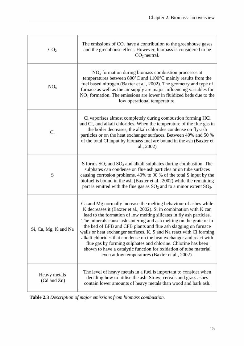
2.6 Emissions The amount of pollutants emitted from biomass is highly dependent on the combustion system and the properties of the fuel. The operating conditions and optimisation of the process also plays an important role, together with additional emission reduction methods used. The highest benefit when comparing biomass to fossil fuel is the reduction of CO2 emitted when using biomass since it is considered to be CO2 neutral. Though, this is only true when the CO2 emitted using fossil fuel during harvesting and transportation is not included. Biomass normally emits less SOx than fossil fuel, due to the low sulphur content. Also NOx emissions are less for biomass. A disadvantage of biomass is the high amount of emissions from incomplete combustion compared to fossil fuel. This is often the case for small scale combustor systems where combustion control systems are not cost- effective. Incomplete combustion leads to a high emission of particulates, i.e soot, char or condensed tar. Table 2.3 contains a description of the major emissions from biomass combustion.
Chapter 2: Biomass- an overview
15
CO2
The emissions of CO2 have a contribution to the greenhouse gases and the greenhouse effect. However, biomass is considered to be
CO2 neutral.
NOx
NOx formation during biomass combustion processes at
temperatures between 800°C and 1100°C mainly results from the fuel based nitrogen (Baxter et al., 2002). The geometry and type of furnace as well as the air supply are major influencing variables for NOx formation. The emissions are lower in fluidized beds due to the
low operational temperature.
Cl
Cl vaporises almost completely during combustion forming HCl
and Cl2 and alkali chlorides. When the temperature of the flue gas in the boiler decreases, the alkali chlorides condense on fly-ash
particles or on the heat exchanger surfaces. Between 40% and 50 % of the total Cl input by biomass fuel are bound in the ash (Baxter et
al., 2002)
S
S forms SO2 and SO3 and alkali sulphates during combustion. The
sulphates can condense on flue ash particles or on tube surfaces causing corrosion problems. 40% to 90 % of the total S input by the biofuel is bound in the ash (Baxter et al., 2002) while the remaining part is emitted with the flue gas as SO2 and to a minor extent SO3.
Si, Ca, Mg, K and Na
Ca and Mg normally increase the melting behaviour of ashes while K decreases it (Baxter et al., 2002). Si in combination with K can lead to the formation of low melting silicates in fly ash particles.
The minerals cause ash sintering and ash melting on the grate or in the bed of BFB and CFB plants and flue ash slagging on furnace
walls or heat exchanger surfaces. K, S and Na react with Cl forming alkali chlorides that condense on the heat exchanger and react with
flue gas by forming sulphates and chlorine. Chlorine has been shown to have a catalytic function for oxidation of tube material
even at low temperatures (Baxter et al., 2002).
Heavy metals (Cd and Zn)
The level of heavy metals in a fuel is important to consider when
deciding how to utilise the ash. Straw, cereals and grass ashes contain lower amounts of heavy metals than wood and bark ash.
Table 2.3 Description of major emissions from biomass combustion.

Diffusion of solid fuel on a vibrating grate
16
Chapter3: Bed models- state of the art
17
3 Bed models- state of the art
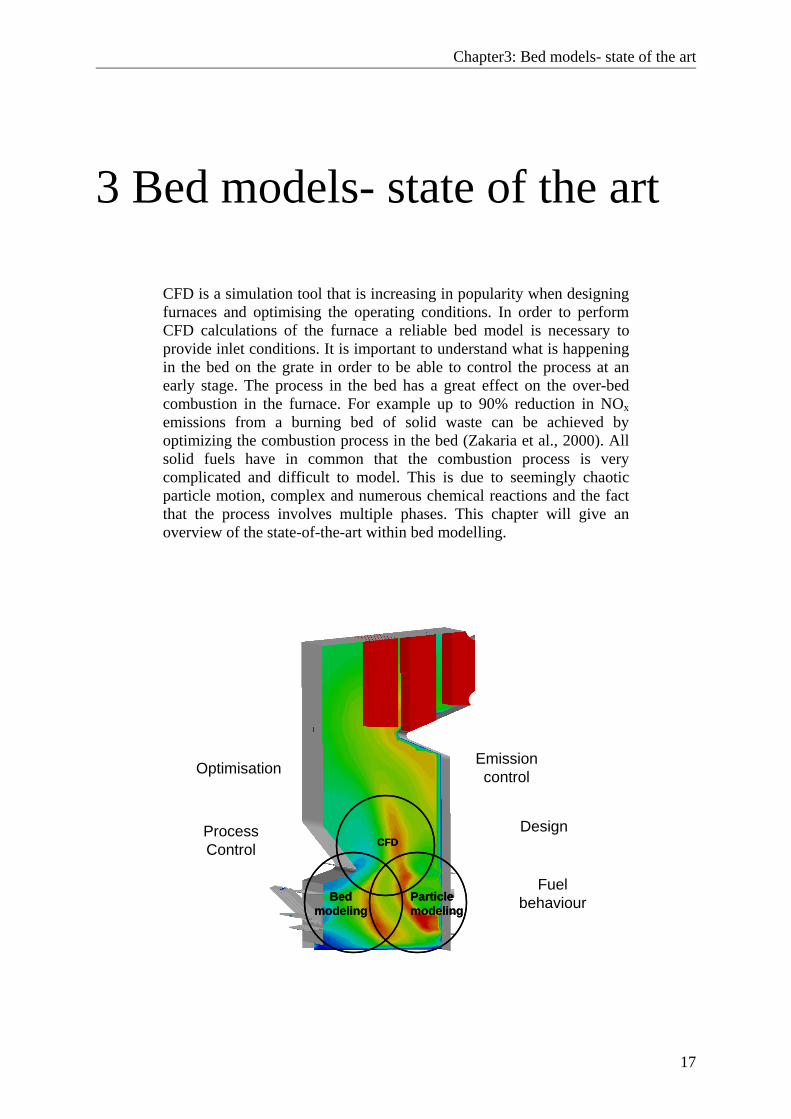
CFD is a simulation tool that is increasing in popularity when designing furnaces and optimising the operating conditions. In order to perform CFD calculations of the furnace a reliable bed model is necessary to provide inlet conditions. It is important to understand what is happening in the bed on the grate in order to be able to control the process at an early stage. The process in the bed has a great effect on the over-bed combustion in the furnace. For example up to 90% reduction in NOx emissions from a burning bed of solid waste can be achieved by optimizing the combustion process in the bed (Zakaria et al., 2000). All solid fuels have in common that the combustion process is very complicated and difficult to model. This is due to seemingly chaotic particle motion, complex and numerous chemical reactions and the fact that the process involves multiple phases. This chapter will give an overview of the state-of-the-art within bed modelling.
CFD
Bed modeling
Particlemodeling
CFD
Bed modeling
Particlemodeling
Optimisation
Design
Emission control
ProcessControl
Fuelbehaviour
Diffusion of solid fuel on a vibrating grate
18
3.1 Kinetics The kinetics of biomass combustion depends on many different factors, e.g. fuel size, fuel composition, surroundings, heat transfer rate etc. According to Di Blasi (1993) the kinetics of biomass conversion can be classified into three groups:
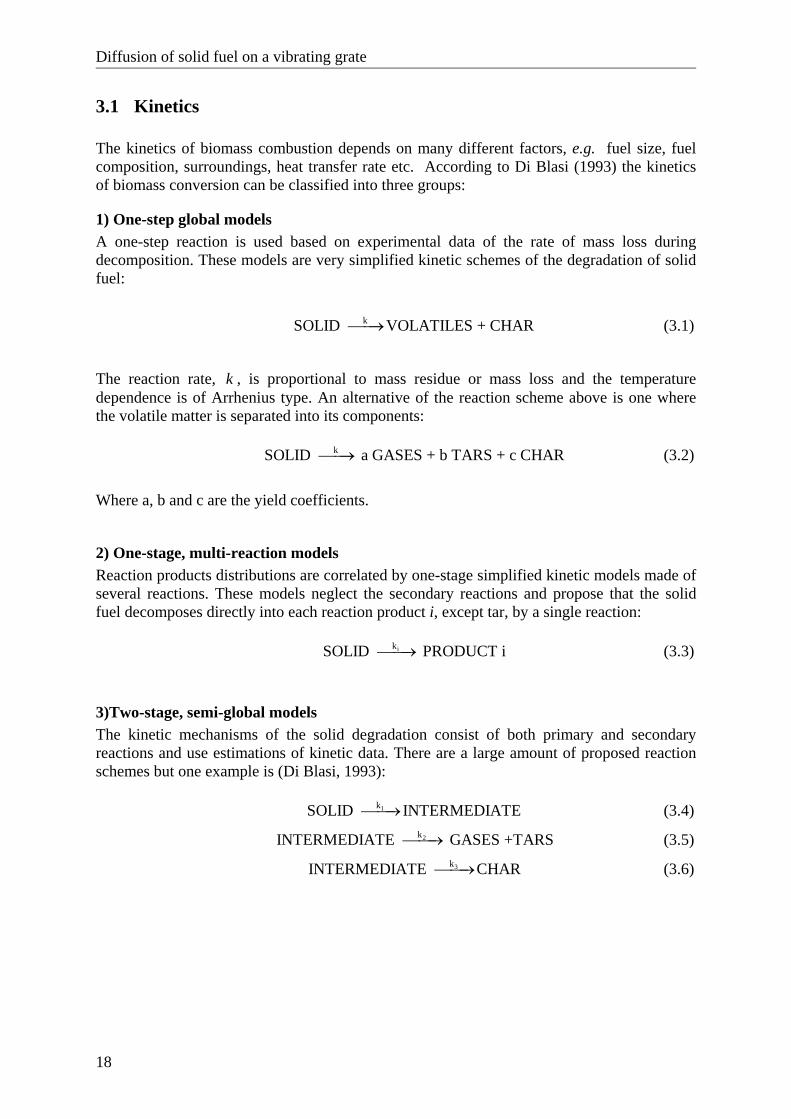
1) One-step global models A one-step reaction is used based on experimental data of the rate of mass loss during decomposition. These models are very simplified kinetic schemes of the degradation of solid fuel:
kSOLID VOLATILES + CHAR⎯⎯→ (3.1)
The reaction rate, k , is proportional to mass residue or mass loss and the temperature dependence is of Arrhenius type. An alternative of the reaction scheme above is one where the volatile matter is separated into its components: kSOLID a GASES + b TARS + c CHAR⎯⎯→ (3.2)
Where a, b and c are the yield coefficients.
2) One-stage, multi-reaction models Reaction products distributions are correlated by one-stage simplified kinetic models made of several reactions. These models neglect the secondary reactions and propose that the solid fuel decomposes directly into each reaction product i, except tar, by a single reaction: ikSOLID PRODUCT i⎯⎯→ (3.3)
3)Two-stage, semi-global models The kinetic mechanisms of the solid degradation consist of both primary and secondary reactions and use estimations of kinetic data. There are a large amount of proposed reaction schemes but one example is (Di Blasi, 1993): 1kSOLID INTERMEDIATE⎯⎯→ (3.4)
2kINTERMEDIATE GASES +TARS⎯⎯→ (3.5)
3kINTERMEDIATE CHAR⎯⎯→ (3.6)
Chapter3: Bed models- state of the art
19
3.2 Modelling of a single particle A large amount of research work, both experimental- and modelling, has been carried out within the combustion of a single particle. The combustion process of a single particle involves many complex sub-processes such as species diffusion, convective transport inside particle, water evaporation and re-condensation, secondary pyrolysis reactions inside the pores, shrinkage and swelling, pore structure etc. To mathematically describe the various processes, assumptions and simplifications are inevitable (Alves and Figueiredo, 1989). Combustion of a single particle is generally divided into two different regimes, a thermally thin and a thermally thick regime. Which one of the regimes to use can be determined by the thermal Biot number, tBi , which relates the internal and external heat transfer rates:
,car c efft
cs
r hBi
k= (3.7)
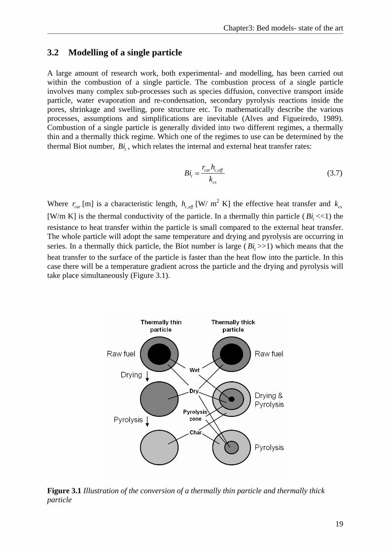
Where carr [m] is a characteristic length, ,c effh [W/ m2 K] the effective heat transfer and csk [W/m K] is the thermal conductivity of the particle. In a thermally thin particle ( tBi <<1) the resistance to heat transfer within the particle is small compared to the external heat transfer. The whole particle will adopt the same temperature and drying and pyrolysis are occurring in series. In a thermally thick particle, the Biot number is large ( tBi >>1) which means that the heat transfer to the surface of the particle is faster than the heat flow into the particle. In this case there will be a temperature gradient across the particle and the drying and pyrolysis will take place simultaneously (Figure 3.1).
Figure 3.1 Illustration of the conversion of a thermally thin particle and thermally thick particle
Diffusion of solid fuel on a vibrating grate
20
Bryden et al. (2002) investigated the pyrolysis of a thermally thick particle and suggested that instead of two regimes there should be three separate pyrolysis regimes based on the particle Biot number: 1) Thermally thin regime (Bi<0.2) 2) Thermally thick regime (0.2<Bi>10) 3) Thermal wave regimes (Bi>10) In the thermally thin regime the temperature is constant in the particle, and both drying and pyrolysis occurs in series. In the thermally thick regime, temperature gradients exist but the reaction rate is slow compared to the heat transfer rate and drying and pyrolysis still occurs in series. For thermal wave regime, drying and pyrolysis regions travel through the particle like a wave (unreacted wood, pyrolysis zone and char exist simultaneously). The model of Bryden et al. (2002) was extended by Hagge and Bryden (2002) to include shrinkage of the particle and later also to include both shrinkage and moisture (Bryden and Hagge, 2003). It was found that shrinkage had a negligible effect on the pyrolysis process in the thermally thin regime. In the thermally thick regime shrinkage was shown to reduce the pyrolysis time by 5-30 %, but had a limited impact on the product yield. In the thermal wave regime shrinkage and moisture effected both the pyrolysis time and the pyrolysis products. Since many applications of biomass combustion involve fuels of larger sizes and thus belong to the thermal wave pyrolysis regime, shrinkage and moisture are two important parameters to consider. A higher moisture content increases the mass flow out of the particle which, in turn, lowers the temperature of the char and reduces the rate of the secondary reactions. The inward movement of the drying and pyrolysis fronts are thereby slowed down. Shrinkage reduces the insulating effect of the char which increases the heat transfer to the drying and pyrolysis zones which results in an increased pyrolysis rate. Thus, higher moisture content increases the pyrolysis time while more shrinkage decreases the time. Increasing moisture and shrinkage work to increase tar yield and decrease the formation of light hydrocarbons. However, shrinkage does not necessarily occur for all types of fuel. Curtis and Miller (1988) reported that during conversion of cellulose no shrinkage was observed, instead it proceeded by an increased porosity of the material. Different shapes of particles were investigated by Thunman et al. (2002) by a one dimensional model for a single wood particle. The model is based on the method of Saastamoinen and Richard (1996) but also includes drying and shrinking of the particle. The results agreed well with experimental measurements carried out in a laboratory scaled fluidised bed, except for devolatilisation time which was slightly overestimated. One reason for this can be that the particles during combustion crack or fall apart which increases the area for heat transfer from surroundings and lower the thermal distance inside the particle. Janse et al. (2000) developed a one-dimensional model of flash pyrolysis of wood with the aim of investigating the effects of heat transfer limitation by out-flowing vapours and intra-particle tar cracking. Incorporation of a pyrolysis-wind effect was shown to increase the conversion time of a particle by up to 40%. The knowledge of the combustion process of a single particle is of great importance when studying the behaviour in a bed, consisting of a large number of particles.
Chapter3: Bed models- state of the art
21
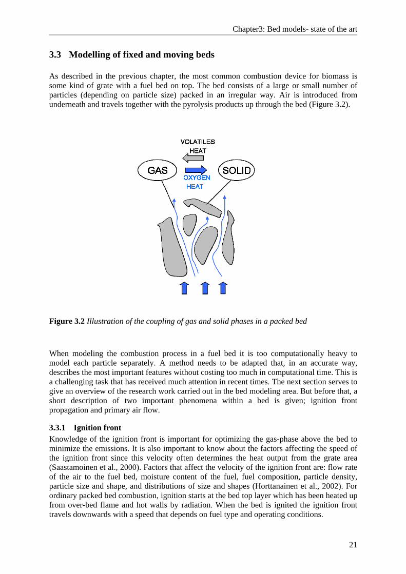
3.3 Modelling of fixed and moving beds As described in the previous chapter, the most common combustion device for biomass is some kind of grate with a fuel bed on top. The bed consists of a large or small number of particles (depending on particle size) packed in an irregular way. Air is introduced from underneath and travels together with the pyrolysis products up through the bed (Figure 3.2).
Figure 3.2 Illustration of the coupling of gas and solid phases in a packed bed
When modeling the combustion process in a fuel bed it is too computationally heavy to model each particle separately. A method needs to be adapted that, in an accurate way, describes the most important features without costing too much in computational time. This is a challenging task that has received much attention in recent times. The next section serves to give an overview of the research work carried out in the bed modeling area. But before that, a short description of two important phenomena within a bed is given; ignition front propagation and primary air flow.
3.3.1 Ignition front Knowledge of the ignition front is important for optimizing the gas-phase above the bed to minimize the emissions. It is also important to know about the factors affecting the speed of the ignition front since this velocity often determines the heat output from the grate area (Saastamoinen et al., 2000). Factors that affect the velocity of the ignition front are: flow rate of the air to the fuel bed, moisture content of the fuel, fuel composition, particle density, particle size and shape, and distributions of size and shapes (Horttanainen et al., 2002). For ordinary packed bed combustion, ignition starts at the bed top layer which has been heated up from over-bed flame and hot walls by radiation. When the bed is ignited the ignition front travels downwards with a speed that depends on fuel type and operating conditions.
Diffusion of solid fuel on a vibrating grate
22
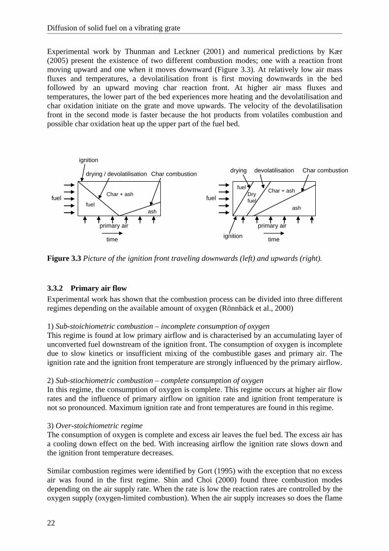
Experimental work by Thunman and Leckner (2001) and numerical predictions by Kær (2005) present the existence of two different combustion modes; one with a reaction front moving upward and one when it moves downward (Figure 3.3). At relatively low air mass fluxes and temperatures, a devolatilisation front is first moving downwards in the bed followed by an upward moving char reaction front. At higher air mass fluxes and temperatures, the lower part of the bed experiences more heating and the devolatilisation and char oxidation initiate on the grate and move upwards. The velocity of the devolatilisation front in the second mode is faster because the hot products from volatiles combustion and possible char oxidation heat up the upper part of the fuel bed.
ignition
fuel
Char + ash
ash
fuel
primary air
fuel
ignition
Dryfuel
Char + ash
ash
time
primary air
fuel
drying devolatilisation Char combustion
time
drying / devolatilisation Char combustion
Figure 3.3 Picture of the ignition front traveling downwards (left) and upwards (right).
3.3.2 Primary air flow Experimental work has shown that the combustion process can be divided into three different regimes depending on the available amount of oxygen (Rönnbäck et al., 2000) 1) Sub-stoichiometric combustion – incomplete consumption of oxygen This regime is found at low primary airflow and is characterised by an accumulating layer of unconverted fuel downstream of the ignition front. The consumption of oxygen is incomplete due to slow kinetics or insufficient mixing of the combustible gases and primary air. The ignition rate and the ignition front temperature are strongly influenced by the primary airflow. 2) Sub-stiochiometric combustion – complete consumption of oxygen In this regime, the consumption of oxygen is complete. This regime occurs at higher air flow rates and the influence of primary airflow on ignition rate and ignition front temperature is not so pronounced. Maximum ignition rate and front temperatures are found in this regime. 3) Over-stoichiometric regime The consumption of oxygen is complete and excess air leaves the fuel bed. The excess air has a cooling down effect on the bed. With increasing airflow the ignition rate slows down and the ignition front temperature decreases. Similar combustion regimes were identified by Gort (1995) with the exception that no excess air was found in the first regime. Shin and Choi (2000) found three combustion modes depending on the air supply rate. When the rate is low the reaction rates are controlled by the oxygen supply (oxygen-limited combustion). When the air supply increases so does the flame
Chapter3: Bed models- state of the art
23
propagation but is limited by the reaction rate of the fuel (reaction-limited combustion). For a further increase of the air supply the excess air cools the bed and quenches the flame (Extinction by convection). Experimental work showed that larger particles allow a larger air flow before flame extinction. This is due to the smaller surface area per unit mass which decreases the cooling effect. Fatehi and Kaviany (1994) identified two combustion modes and called them an oxygen-limited and a fuel-limited mode. The oxygen-limited mode corresponds to the above described sub-stoichiometric regimes and the fuel-limited one to the over-stoichiometric regime.
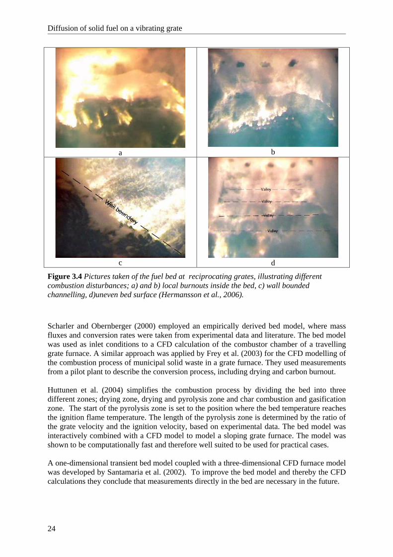
3.4 Bed models In grate furnaces there are often instability problems of the combustion process in the fuel bed. Some frequently occurring problems are local burnouts in the fuel bed, i.e areas of intensified combustion, and channelling, where primary air flow by-passes through the bed without reacting with the fuel. Hermansson et al. (2006) have made an inventory of the disturbances taking place in ten different grate furnaces of sizes from 8 MWth to 32 MWth. The inventory was carried out by interviewing the personnel responsible for the operation of the furnaces and by recording the fuel bed with a video camera. The results showed that all furnaces, except one, experienced combustion disturbances. The disturbances consisted of wall-bounded channelling, burnouts inside the bed, skewed flame front due to uneven bed surfaces and material break-down of the grate rods. The different phenomena are illustrated in Figure 3.4. The combustion disturbances motivate the need of developing models in order to increase the understanding of the combustion process and preventing these types of problems. The pictures shown in Figure 3.4 also illustrate the complexity of the burning of biomass and thereby the difficulties in the modelling work. In order to describe the combustion of biomass in a bed, approximations of the process are necessary. Göerner (2003) has identified five different model levels: 1. Zero-dimensional model
A model where the heat release and the released species are assumed by integral assumption. The biomass conversion is uniform along the grate length and width.
2. One-dimensional model
Heat release and species concentrations profiles are calculated over the length of the grate. The conversion across the grate is assumed to be uniform. To get the profile at the top of the bed, overall mass and energy balances are solved.
3. One-dimensional transient model
In addition to the model described above, the burnout progress in the vertical direction is also included
4. Two-dimensional model
The conversion process is modelled both across and along the grate.
5. Three-dimensional model A fully three-dimensional model solves the conversion process in all three directions.
Diffusion of solid fuel on a vibrating grate
24
a
b
c
d
Figure 3.4 Pictures taken of the fuel bed at reciprocating grates, illustrating different combustion disturbances; a) and b) local burnouts inside the bed, c) wall bounded channelling, d)uneven bed surface (Hermansson et al., 2006).
Scharler and Obernberger (2000) employed an empirically derived bed model, where mass fluxes and conversion rates were taken from experimental data and literature. The bed model was used as inlet conditions to a CFD calculation of the combustor chamber of a travelling grate furnace. A similar approach was applied by Frey et al. (2003) for the CFD modelling of the combustion process of municipal solid waste in a grate furnace. They used measurements from a pilot plant to describe the conversion process, including drying and carbon burnout. Huttunen et al. (2004) simplifies the combustion process by dividing the bed into three different zones; drying zone, drying and pyrolysis zone and char combustion and gasification zone. The start of the pyrolysis zone is set to the position where the bed temperature reaches the ignition flame temperature. The length of the pyrolysis zone is determined by the ratio of the grate velocity and the ignition velocity, based on experimental data. The bed model was interactively combined with a CFD model to model a sloping grate furnace. The model was shown to be computationally fast and therefore well suited to be used for practical cases. A one-dimensional transient bed model coupled with a three-dimensional CFD furnace model was developed by Santamaria et al. (2002). To improve the bed model and thereby the CFD calculations they conclude that measurements directly in the bed are necessary in the future.
Chapter3: Bed models- state of the art
25
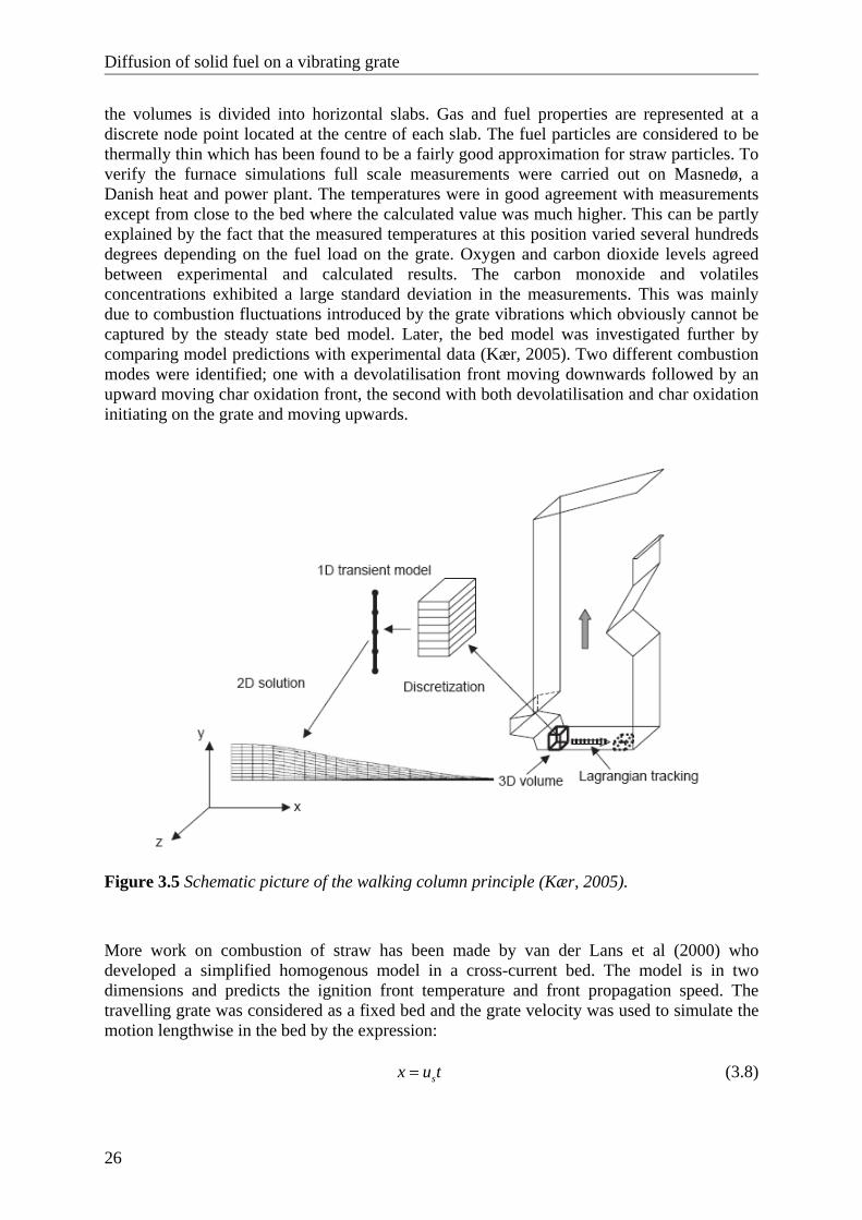
Like for a single particle, the modelling work can be simplified by assuming thermally thin particles. However, for a packed bed the heating conditions are different from the case of a single particle since the radiation from the ignition flame can only penetrate the bed through voids in between the particles. Yang et al. (2005a) stated that the definition of the Biot number for a single particle needs to be modified and should be proportional to the local bed voidage. They also found that particles in a packed bed can be treated as thermally thin for a size less than 30mm. If thermally thin particles can be assumed, the temperature inside the particles is uniform and the whole bed can be assumed as a continuous porous medium with two phases, one solid and one gas phase. Bruch et al. (2003) developed a bed model describing the conversion of wood under fixed bed conditions. The bed consists of a finite number of particles of various sizes, the conversion of each particle is described by a one-dimensional transient model. Results showed that a description of the heat and mass transfer within each solid particle was not necessary for the conversion of char only. However, for a model that can be applied to the whole conversion process, transport processes within the particle cannot be neglected. For many applications though, it is not possible to treat the particles as thermally thin and a more detailed model is necessary. Thunman and Leckner (2003) use a model for the conversion of a thermally thick single particle (Thunman et al., 2002) to develop a bed model that can be applied to batch-fired combustors, continuously operating co-current or counter-current combustors and moving grates. For the case of a moving grate the model describes the combustion of a fuel batch transported along the grate, where time is translated into a distance along the grate. The bed consists of equally sized thermally thick particles of various shapes. The case of fuel batch combustion was compared to measurements collected from the literature with satisfactory agreement on the rate of propagation and thickness of the conversion front. The bed model has been used later to investigate the influence of density and particle size on the combustion of a packed bed (Thunman and Leckner, 2005b). Experiments and modelling showed that the particle size has a significant influence on the conversion process. In a bed with large particles, there was a clear temperature difference between the gas and the solid surface, and the conversion processes for drying, devolatilisation and char combustion overlapped. For small particles the gas temperature and particle surface temperature were almost the same and the conversion processes sequential. This agrees with the discussion above about the possible simplification of the bed modelling by treating the bed as a porous continuous media for small particles. The model also showed that the density of the fuel does not have a significant effect on the conversion rate if the conversion rate is related to the mass loss per unit time and cross sectional area of the bed. This means that experiences from one fuel density can be used directly for similar fuels but with different densities. Shin and Choi (2000) made the assumption that the heat and mass transfer in the direction of movement of the bed can be ignored since the gradients of temperatures and concentration of chemical species in this direction are negligible compared to those in the direction of the gas flow. It resulted in a one-dimensional transient model, often referred to as a walking column model, where the evaporation and combustion zones travels from the top of the bed to the bottom until only ash remains. Kær (2004) also used a walking column approach (Figure 3.5) when developing a bed model to be used as boundary conditions to CFD calculations of a 33MW straw-fired boiler with a vibrating grate. The bed model considers the fuel layer as a number of 3D volumes. Each of
Diffusion of solid fuel on a vibrating grate
26
the volumes is divided into horizontal slabs. Gas and fuel properties are represented at a discrete node point located at the centre of each slab. The fuel particles are considered to be thermally thin which has been found to be a fairly good approximation for straw particles. To verify the furnace simulations full scale measurements were carried out on Masnedø, a Danish heat and power plant. The temperatures were in good agreement with measurements except from close to the bed where the calculated value was much higher. This can be partly explained by the fact that the measured temperatures at this position varied several hundreds degrees depending on the fuel load on the grate. Oxygen and carbon dioxide levels agreed between experimental and calculated results. The carbon monoxide and volatiles concentrations exhibited a large standard deviation in the measurements. This was mainly due to combustion fluctuations introduced by the grate vibrations which obviously cannot be captured by the steady state bed model. Later, the bed model was investigated further by comparing model predictions with experimental data (Kær, 2005). Two different combustion modes were identified; one with a devolatilisation front moving downwards followed by an upward moving char oxidation front, the second with both devolatilisation and char oxidation initiating on the grate and moving upwards.
Figure 3.5 Schematic picture of the walking column principle (Kær, 2005).
More work on combustion of straw has been made by van der Lans et al (2000) who developed a simplified homogenous model in a cross-current bed. The model is in two dimensions and predicts the ignition front temperature and front propagation speed. The travelling grate was considered as a fixed bed and the grate velocity was used to simulate the motion lengthwise in the bed by the expression:
sx u t= (3.8)
Chapter3: Bed models- state of the art
27
Where x [m] is the position on the grate and su [m/s] is the bed transport velocity. This simplification is valid when the heat transport by conduction in the horizontal direction is much smaller than the heat flux by the transport of the bed itself. This can be expressed by the Peclet number, Pe. Heat transport by convection can be neglected for Pe>>1. For straw combustion on a travelling grate the Pe number was found to be of the order of 104 for heat transportation in the horizontal direction. By using this assumption the two-dimensional steady-state bed model was transformed into a transient one-dimensional model. To validate the model, experimental work with a laboratory fixed bed combustor, was carried out. The fuel was ignited from the top and the reaction front moved downward in the bed. After the ignition front reached the grate a burnout front could be detected moving in the opposite direction, from the grate upwards. The bed maintained its original structure throughout the burning process. The results from the model were in fairly good agreement with the experimental results but with an over predicted ignition rate and reaction front temperature. The modelling work of van der Lans et al. has later been improved and extended from being a homogenous model to be a heterogeneous model by Zhou et al. (2005). The model provided detailed structure of the ignition flame front, gas species concentrations at the bed surface, ignition flame front rate and temperature. The modelling results showed that the bed is in a fuel rich condition, since a higher air flow gives a higher bed temperature (more oxygen provided. The packing conditions had a significant impact on the combustion behaviour in the fixed bed. A variation of 15% porosity resulted in variations of 10% of the ignition flame front rate and 1.5% of the bed temperature. Simulations also showed that the effect of straw heat capacity on the ignition flame front rate is significant. A variation of 25% of the heat capacity results in a variation of about 10% of the ignition flame front rate and temperature less than 2%. Simulations showed that the effects of the mass and heat transfer coefficients on the ignition flame front rate are weak. Waste is a complicated biomass fuel due to a large variation in particle size and chemical composition. To be able to numerically model the combustion process in the bed would be of great help in understanding the process and thereby designing and optimising the incinerating equipment. Yang et al. (2002) have been working on modelling of waste incineration on a moving grate which has resulted in a graphically interactive computer program, The Fluid Dynamic Incinerator Code (FLIC). The model is in two dimensions and the method based on the governing equations for packed beds proposed by Peters (2003). The bed and the freeboard area above are divided into many small volumes, the transport equations concerning the flow, heat transfer and combustion of the solid and gas phases are then discretised over these volumes, and solved iteratively over the whole computation domain. During measurements on a test scale cylindrical combustion chamber large fluctuations in species concentration were observed as a result of channelling phenomenon in the bed. The numerical simulations, without considering the channelling effects, showed good agreement regarding mass loss but significant discrepancy for temperature and gas composition profiles. Mixing of the fuel particles is taken into account by a diffusion coefficient in the conservation equation for the solid-phase species (Yang et al., 2005b). The horizontal particle velocity is given a predetermined value and the vertical velocity calculated through the continuity equation. The diffusion coefficients are based on experimental work carried out on scaled test rigs (Lim et al, 2001). The modelling work by Yang et al. has later been followed by a series of theoretical studies on the effect of fuel moisture, devolatilisation rate and primary air velocity (Yang et al., 2003a, Yang et al. 2003b, Yang et al. 2004). Measurements inside a full-scale incinerator have been carried out by an in-house instrument that is fed onto the grate together with the waste and recording temperature, gas composition and bed motion
Diffusion of solid fuel on a vibrating grate
28
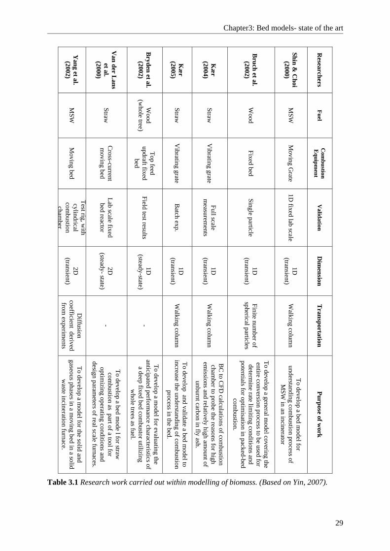
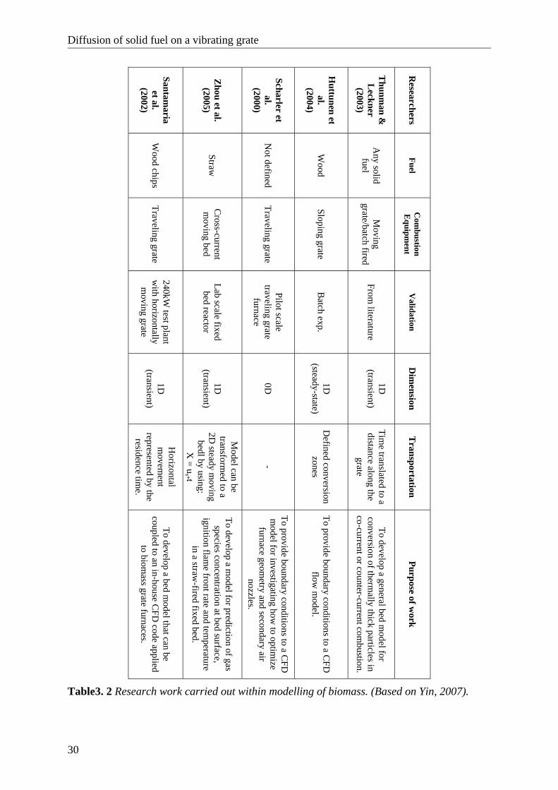
(Yang et al. 2005c). It could be seen that bed fluctuations in temperature and O2 were related to the movement of the grate indicating the importance of an accurate model for mixing of the fuel. Finally, an illustrative example of the usage of bed modelling is the work of Bryden and Ragland (1996). A one-dimensional steady-state bed model was developed with the purpose of providing information about the combustion process for the design of a new type of combustor. The idea was to grow hard wood trees, such as hybrid poplars, and then harvest the whole trees and introducing them into a deep bed, top feed updraft combustor. The model results showed a great flexibility of parameters that can be altered in order to achieve the desired power output. The flexibility was of significant importance in the design work and planned operation. Table 3.1 and 3.2 summarise the different model approaches described in this chapter.
Chapter3: Bed models- state of the art
29
Yang et al. (2002)
Van der L
ans et al.
(2000)
Bryden et al.
(2002)
Kæ
r (2005)
Kæ
r (2004)
Bruch et al. (2002)
Shin & C
hoi (2000)
Researchers
MSW
Straw
Wood
(whole tree)
Straw
Straw
Wood
MSW
Fuel
Moving bed
Cross-current
moving bed
Top feed updraft fixed
bed
Vibrating grate
Vibrating grate
Fixed bed
Moving G
rate
Com
bustion E
quipment
Test rig, with
cylindrical com
bustion cham
ber
Lab scale fixed bed reactor
Field test results
Batch exp.
Full scale m
easurements
Single particle
1D fixed lab scale
Validation
2D
(transient)
2D
(steady- state)
1D
(steady-state)
1D
(transient)
1D
(transient)
1D
(transient)
1D
(transient)
Dim
ension
Diffusion
coefficient derived from
experiments
- -
Walking colum
n
Walking colum
n
Finite number of
spherical particles
Walking colum
n
Transportation
To develop a model for the solid and
gaseous phases in a moving bed in a solid
waste incineration furnace.
To develop a bed mode l for straw
com
bustion as part of a tool for optim
izing operating conditions and design param
eters of real scale furnaces.
To develop a model for evaluating the
anticipated performance characteristics of
a deep fixed bed combustor utilizing
whole trees as fuel.
To develop and validate a bed model to
increase the understanding of combustion
process in the bed.
BC
to CFD
calculations of combustion
chamber to probe the reasons for high
emissions and relatively high am
ount of unburnt carbon in fly ash.
To develop a general model covering the
entire conversion process to be used for determ
ine rate limiting conditions and
potentials for optimisation in packed-bed
combustion.
To develop a bed model for
understanding combustion process of
MSW
in an incinerator
Purpose of work
Table 3.1 Research work carried out within modelling of biomass. (Based on Yin, 2007).
Diffusion of solid fuel on a vibrating grate
30
Santamaria
et al. (2002)
Zhou et al. (2005)
Scharler et al.
(2000)
Huttunen et
al. (2004)
Thunm
an &
Leckner (2003)
Researchers
Wood chips
Straw
Not defined
Wood
Any solid fuel
Fuel
Traveling grate
Cross-current
moving bed
Traveling grate
Sloping grate
Moving
grate/batch fired
Com
bustion E
quipment
240kW test plant
with horizontally m
oving grate
Lab scale fixed bed reactor
Pilot scale traveling grate
furnace
Batch exp.
From literature
Validation
1D
(transient)
1D
(transient)
0D
1D
(steady-state)
1D
(transient)
Dim
ension
Horizontal
movem
ent represented by the
residence time.
Model can be
transformed to a
2D steady m
oving bedl by using:
X = u
s* t
-
Defined conversion
zones
Time translated to a
distance along the grate
Transportation
To develop a bed model that can be
coupled to an in-house CFD
code applied to biom
ass grate furnaces.
To develop a model for prediction of gas
species concentration at bed surface, ignition flam
e front rate and temperature
in a straw-fired fixed bed.
To provide boundary conditions to a CFD
m
odel for investigating how to optim
ize furnace geom
etry and secondary air nozzles.
To provide boundary conditions to a CFD
flow
model.
To develop a general bed model for
conversion of thermally thick particles in
co-current or counter-current combustion.
Purpose of work
Table3. 2 Research work carried out within modelling of biomass. (Based on Yin, 2007).
Chapter 4: Mixing theory of particles
31
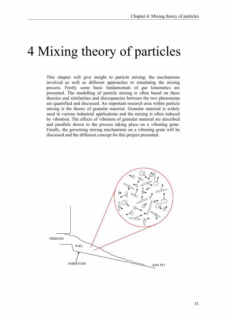
4 Mixing theory of particles
This chapter will give insight to particle mixing; the mechanisms involved as well as different approaches to simulating the mixing process. Firstly some basic fundamentals of gas kinematics are presented. The modelling of particle mixing is often based on these theories and similarities and discrepancies between the two phenomena are quantified and discussed. An important research area within particle mixing is the theory of granular material. Granular material is widely used in various industrial applications and the mixing is often induced by vibration. The effects of vibration of granular material are described and parallels drawn to the process taking place on a vibrating grate. Finally, the governing mixing mechanisms on a vibrating grate will be discussed and the diffusion concept for this project presented.
FEEDING
VIBRATION
FUEL
ASH PIT
Diffusion of solid fuel on a vibrating grate
32
4.1 Gas kinetic theory The gas kinetic theory yields transport coefficients from the fundamental properties of the gas molecules. A gas contains many molecule particles moving in different directions and at different speeds. Collisions between the particles change their speed and direction. The particles are too small to be seen by eye but obey the classical laws of matter. The motion of the molecules is described by probability functions and not by their individual paths. The kinetic theory of gases is based on three fundamental approximations, which are: 1. Molecular hypothesis The molecular hypothesis assumes that matter is composed of small discrete units; molecules. All molecules of a given substance are alike, and the states of matter differ essentially in the arrangement and state of motion of the molecules. Gases differ from solids and liquids by completely filling any container in which they are placed, by rapidly diffusing into one another and by having very low densities. The molecules in a gas are widely separated from one another and they move around freely throughout the entire space occupied by the gas. There is no friction involved in molecular interactions. 2. Classical conservation laws can be applied Relativistic corrections, quantum mechanics and non-ideal gas effects are usually not considered in the classical kinetic theory of gases. 3. Application of statistical methods Gas kinetic theory involves the description of a very large number of individual molecules by statistical methods. The number of molecules is far too big to consider the dynamics of each single molecule. It is only necessary to know so much about the molecular motion as is necessary to understand and predict the observable, macroscopic properties of the gas.
4.2 Maxwell-Boltzmann distribution function It is possible to develop connections between the motion of microscopic molecules and the observable macroscopic properties with help of Maxwell-Boltzmanns’s distribution function. The function is a probability distribution and is often referred to as the molecular speed in a gas but, it can also refer to distribution of other properties, such as velocities and momentum of the molecules. The function was derived in 1859 and is only valid for gases in thermodynamic equilibrium. The Maxwell-Boltzmann distribution can be derived using statistical mechanics with the following assumptions:
• The gas is composed of an indefinite number of small, hard and perfectly elastic spheres acting on one another only during impact. When two spheres collide, their direction after the collision is distributed with equal probability over all angles.
• At any spatial location the distribution of molecular velocities is independent of
time.
• After a number of collisions the orthogonal components of the molecular velocities are statistically independent.
Chapter 4: Mixing theory of particles
33
• The distribution function is isotropic, i.e. there is no preferred direction and the
distribution function is independent of the orientation of the coordinate system.
4.3 Brownian motion Any of various physical phenomena in which some quantity is constantly undergoing small random fluctuations is called Brownian motion. If a number of particles are present in a given medium the particles will, over a period of time, spread evenly throughout the medium. A higher temperature leads to a more rapid Brownian motion. Diffusion is a macroscopic manifestation of Brownian motion on the microscopic level. In next section the diffusion theory are described and the equations involved presented.
4.4 Diffusion Mass transfer by diffusion refers to movement of molecular species relatively to another. Diffusion can result from pressure gradients (pressure diffusion), temperature gradients (thermal diffusion), external force fields (forced diffusion) and concentration gradients. The primary effect is diffusion caused by concentration gradients, also called ordinary diffusion. Ordinary diffusion is described by Fick’s law:
CJ Dx
∂=
∂ (4.1)
Where J is the diffusion flux, D the diffusion coefficient, C is the concentration and x is the distance.
4.4.1 Transport equation To describe diffusion numerically, the transport equation is applied. If ml is the mass fraction of a chemical species the conservation of ml is expressed as:
( ) ( )ll l l
mdiv m R
tρ
ρ∂
+ + =∂
u J (4.2)
where: ( )lm
tρ∂∂
is the rate of change of the mass of the chemical species per unit
volume
lmρu is the convection flux of species, flux carried by the general flow field
lJ is the diffusion flux, normally caused by the gradients of ml
Diffusion of solid fuel on a vibrating grate
34
lR is the rate of generation of the chemical species per unit volume. The generation is caused by chemical reactions.
If the diffusion flux is expressed through Fick’s law of diffusion, it can be expressed by Eq. (4.1.) The diffusion coefficient will generally be a function of pressure, temperature, and chemical composition. Liquid and solid diffusivities are strongly concentration dependent and generally increase with temperature. The equation of diffusion is on the same form as the equation of conduction of heat: it indicates a progress or spreading out of the gas, similar to the progress and spreading of heat in a problem of conduction. The larger the diffusion coefficient is, the more rapidly this progress takes place. The diffusion coefficient is largest when the free paths are longest, and vice versa. Long free paths mean rapid diffusion, as should be expected.
4.5 Particle mixing Particle mixing is widely used in industry. Whenever particulate matter is processed there is normally some kind of mixing involved. The mixing process is greatly influenced by the flow characteristics of the particles to be mixed. The flow characteristics are, in turn, a result of the type of particles and the way the mixing is induced. The four major types of mixing equipment are tumbler, hopper (gravity driven), convective and fluidized mixers. Mixtures of particles can be divided into two different groups: free-flowing particles and cohesive mixtures (Fan and Chen, 1990). A free-flowing mixture will generally permit the individual particles to move independently, whilst particles in a cohesive mixture move in clusters of particles as a result of present inter-particulate bonding mechanisms. In free-moving mixtures the mixing process is statistical or stochastic and the rules of probability apply. Barker and Metha (1993) have shown that the change between independent particle motion and collective motions takes place in the regime where the voidage between the particles are of approximately the same size as the particles. For a collection of identical particles a completely random mixture can be obtained. If the particles are non-identical only a partial random mixture will be obtained due to incomplete mixing or segregation of the particles. This leads to an inhomogeneous distribution of the individual particles in the mixture. The homogeneity of a mixture is normally indicated by a mixing index. Particle motion can either be described by an Eulerian or Langrangian approach. The Lagrangian approach considers each single particle and its interaction with surrounding particles. This requires detailed information about the particle properties and composition. The Eulerian approach treats the particles as a single group which reduces the required information and simplifies the calculations.
4.6 Granular flow Granular materials are complex systems of a large number of particles of various size, shape and material. The motion of each particle is defined by classical Newtonian mechanisms and
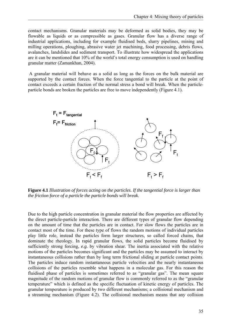
Chapter 4: Mixing theory of particles
35
contact mechanisms. Granular materials may be deformed as solid bodies, they may be flowable as liquids or as compressible as gases. Granular flow has a diverse range of industrial applications, including for example fluidised beds, slurry pipelines, mining and milling operations, ploughing, abrasive water jet machining, food processing, debris flows, avalanches, landslides and sediment transport. To illustrate how widespread the applications are it can be mentioned that 10% of the world’s total energy consumption is used on handling granular matter (Zamankhan, 2004). A granular material will behave as a solid as long as the forces on the bulk material are supported by the contact forces. When the force tangential to the particle at the point of contact exceeds a certain fraction of the normal stress a bond will break. When the particle-particle bonds are broken the particles are free to move independently (Figure 4.1).
Ft < Ff Ft > Ff
Ff
Ft
Ft
Ff
Ft = Ftangential
Ff= Ffriction
Ft = Ftangential
Ff= Ffriction
Figure 4.1 Illustration of forces acting on the particles. If the tangential force is larger than the friction force of a particle the particle bonds will break.
Due to the high particle concentration in granular material the flow properties are affected by the direct particle-particle interaction. There are different types of granular flow depending on the amount of time that the particles are in contact. For slow flows the particles are in contact most of the time. For these type of flows the random motions of individual particles play little role, instead the particles form larger structures, so called forced chains, that dominate the rheology. In rapid granular flows, the solid particles become fluidised by sufficiently strong forcing, e.g. by vibration shear. The inertia associated with the relative motions of the particles becomes significant and the particles may be assumed to interact by instantaneous collisions rather than by long term frictional sliding at particle contact points. The particles induce random instantaneous particle velocities and the nearly instantaneous collisions of the particles resemble what happens in a molecular gas. For this reason the fluidised phase of particles is sometimes referred to as “granular gas”. The mean square magnitude of the random motions of granular flow is commonly referred to as the “granular temperature” which is defined as the specific fluctuation of kinetic energy of particles. The granular temperature is produced by two different mechanisms; a collisional mechanism and a streaming mechanism (Figure 4.2). The collisional mechanism means that any collision
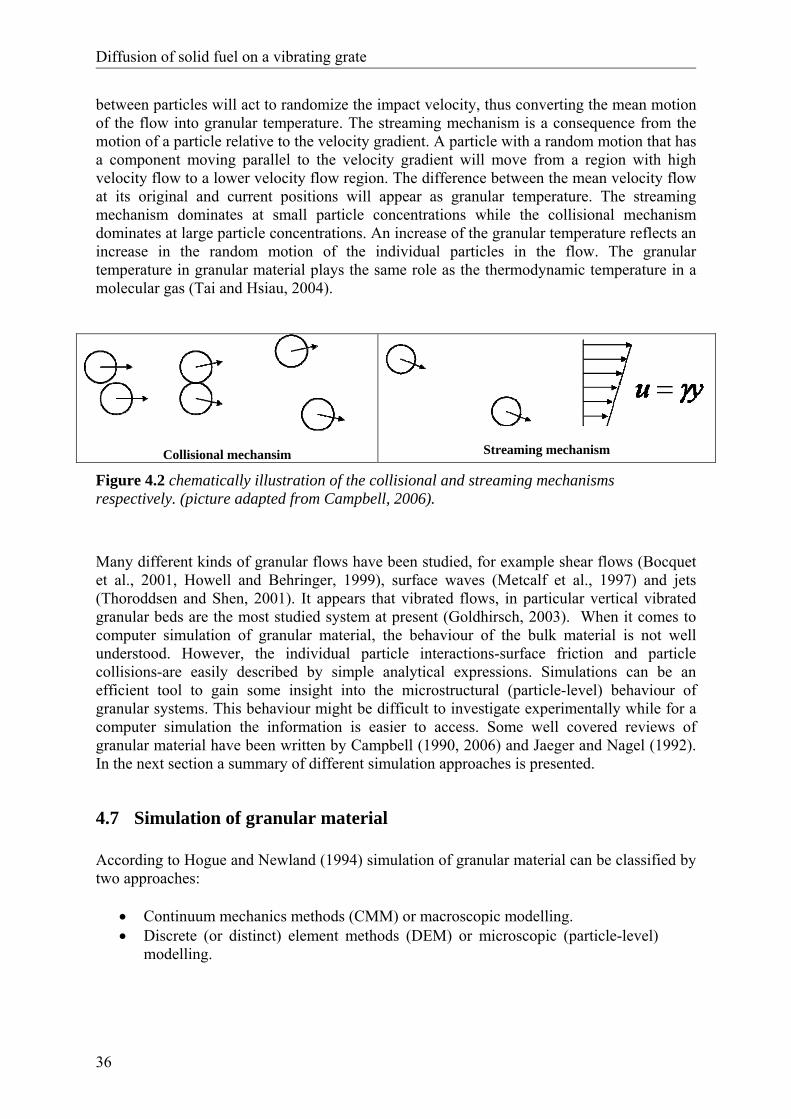
Diffusion of solid fuel on a vibrating grate
36
between particles will act to randomize the impact velocity, thus converting the mean motion of the flow into granular temperature. The streaming mechanism is a consequence from the motion of a particle relative to the velocity gradient. A particle with a random motion that has a component moving parallel to the velocity gradient will move from a region with high velocity flow to a lower velocity flow region. The difference between the mean velocity flow at its original and current positions will appear as granular temperature. The streaming mechanism dominates at small particle concentrations while the collisional mechanism dominates at large particle concentrations. An increase of the granular temperature reflects an increase in the random motion of the individual particles in the flow. The granular temperature in granular material plays the same role as the thermodynamic temperature in a molecular gas (Tai and Hsiau, 2004).
Collisional mechansim
Streaming mechanism
Figure 4.2 chematically illustration of the collisional and streaming mechanisms respectively. (picture adapted from Campbell, 2006).
Many different kinds of granular flows have been studied, for example shear flows (Bocquet et al., 2001, Howell and Behringer, 1999), surface waves (Metcalf et al., 1997) and jets (Thoroddsen and Shen, 2001). It appears that vibrated flows, in particular vertical vibrated granular beds are the most studied system at present (Goldhirsch, 2003). When it comes to computer simulation of granular material, the behaviour of the bulk material is not well understood. However, the individual particle interactions-surface friction and particle collisions-are easily described by simple analytical expressions. Simulations can be an efficient tool to gain some insight into the microstructural (particle-level) behaviour of granular systems. This behaviour might be difficult to investigate experimentally while for a computer simulation the information is easier to access. Some well covered reviews of granular material have been written by Campbell (1990, 2006) and Jaeger and Nagel (1992). In the next section a summary of different simulation approaches is presented.
4.7 Simulation of granular material According to Hogue and Newland (1994) simulation of granular material can be classified by two approaches:
• Continuum mechanics methods (CMM) or macroscopic modelling. • Discrete (or distinct) element methods (DEM) or microscopic (particle-level)
modelling.
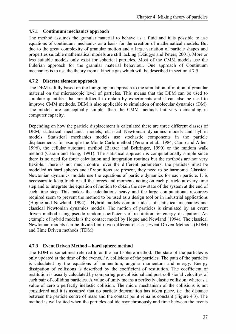
Chapter 4: Mixing theory of particles
37
4.7.1 Continuum mechanics approach The method assumes the granular material to behave as a fluid and it is possible to use equations of continuum mechanics as a basis for the creation of mathematical models. But due to the great complexity of granular motion and a large variation of particle shapes and properties suitable mathematical models are still lacking (Džiugys and Peters, 2001). More or less suitable models only exist for spherical particles. Most of the CMM models use the Eulerian approach for the granular material behaviour. One approach of Continuum mechanics is to use the theory from a kinetic gas which will be described in section 4.7.5.
4.7.2 Discrete element approach The DEM is fully based on the Langrangian approach to the simulation of motion of granular material on the microscopic level of particles. This means that the DEM can be used to simulate quantities that are difficult to obtain by experiments and it can also be used to improve CMM methods. DEM is also applicable to simulation of molecular dynamics (DM). The models are conceptually simpler than the CMM methods but very demanding in computer capacity. Depending on how the particle displacement is calculated there are three different classes of DEM; statistical mechanics models, classical Newtonian dynamics models and hybrid models. Statistical mechanics models use stochastic components in the particle displacements, for example the Monte Carlo method (Perram et al., 1984, Camp and Allen, 1996), the cellular automata method (Baxter and Behringer, 1990) or the random walk method (Caram and Hong, 1991). The statistical approach is computationally simple since there is no need for force calculation and integration routines but the methods are not very flexible. There is not much control over the different parameters, the particles must be modelled as hard spheres and if vibrations are present, they need to be harmonic. Classical Newtonian dynamics models use the equations of particle dynamics for each particle. It is necessary to keep track of all the forces and moments acting on each particle at every time step and to integrate the equation of motion to obtain the new state of the system at the end of each time step. This makes the calculations heavy and the large computational resources required seem to prevent the method to be used as a design tool or in industrial applications (Hogue and Newland, 1994). Hybrid models combine ideas of statistical mechanics and classical Newtonian dynamics models. The motion of particles is simulated by an event driven method using pseudo-random coefficients of restitution for energy dissipation. An example of hybrid models is the contact model by Hogue and Newland (1994). The classical Newtonian models can be divided into two different classes; Event Driven Methods (EDM) and Time Driven methods (TDM).
4.7.3 Event Driven Method – hard sphere method The EDM is sometimes referred to as the hard sphere method. The state of the particles is only updated at the time of the events, i.e. collisions of the particles. The path of the particles is calculated by the equations of momentum, angular momentum and energy. Energy dissipation of collisions is described by the coefficient of restitution. The coefficient of restitution is usually calculated by comparing pre-collisional and post-collisional velocities of each pair of colliding particles. A value of unity means a perfectly elastic collision, whereas a value of zero a perfectly inelastic collision. The micro mechanism of the collisions is not considered and it is assumed that no particle deformation has taken place, i.e. the distance between the particle centre of mass and the contact point remains constant (Figure 4.3). The method is well suited when the particles collide asynchronously and time between the events
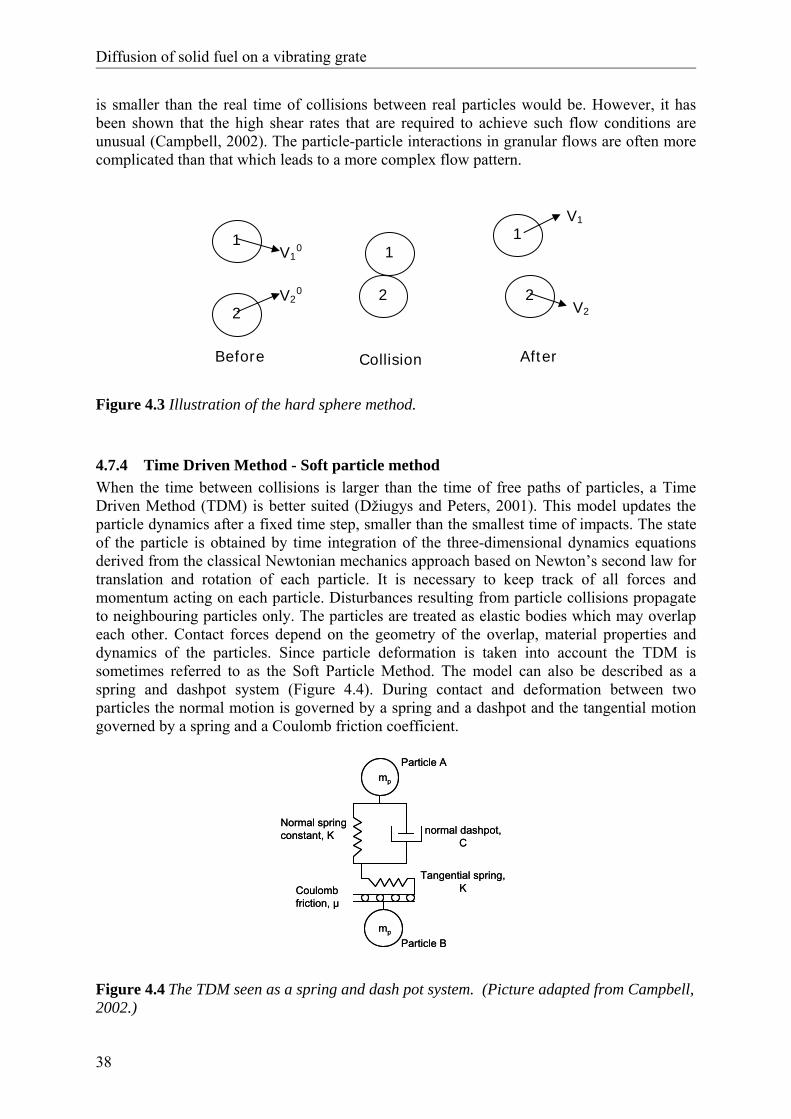
Diffusion of solid fuel on a vibrating grate
38
is smaller than the real time of collisions between real particles would be. However, it has been shown that the high shear rates that are required to achieve such flow conditions are unusual (Campbell, 2002). The particle-particle interactions in granular flows are often more complicated than that which leads to a more complex flow pattern.
Figure 4.3 Illustration of the hard sphere method.
4.7.4 Time Driven Method - Soft particle method When the time between collisions is larger than the time of free paths of particles, a Time Driven Method (TDM) is better suited (Džiugys and Peters, 2001). This model updates the particle dynamics after a fixed time step, smaller than the smallest time of impacts. The state of the particle is obtained by time integration of the three-dimensional dynamics equations derived from the classical Newtonian mechanics approach based on Newton’s second law for translation and rotation of each particle. It is necessary to keep track of all forces and momentum acting on each particle. Disturbances resulting from particle collisions propagate to neighbouring particles only. The particles are treated as elastic bodies which may overlap each other. Contact forces depend on the geometry of the overlap, material properties and dynamics of the particles. Since particle deformation is taken into account the TDM is sometimes referred to as the Soft Particle Method. The model can also be described as a spring and dashpot system (Figure 4.4). During contact and deformation between two particles the normal motion is governed by a spring and a dashpot and the tangential motion governed by a spring and a Coulomb friction coefficient.
normal dashpot, C
Tangential spring, K
Normal spring constant, K
Coulomb friction, μ
mp
mp
Particle A
Particle B
normal dashpot, C
Tangential spring, K
Normal spring constant, K
Coulomb friction, μ
mp
mp
Particle A
Particle B
Figure 4.4 The TDM seen as a spring and dash pot system. (Picture adapted from Campbell, 2002.)
1
2 2
1
2
1 V1
0
V20
V1
V2
Collision Before After
Chapter 4: Mixing theory of particles
39
4.7.5 Kinetic theory approach A popular approach when simulating granular material is to apply theory from the kinetic theory and look at granular flow as a diffusive process. Hisau and Hunt (1992), Natarajan et al. (1995) and Zik and Stavans (1991) all found that the concentration could be fitted to the results of a diffusion equation and concluded that granular mixing is a diffusion process. When a system is seen as diffusive, the particle displacements can be related to the coefficient of self-diffusion D , by the kinematic expression (Natarajan et al., 1995): 2lim 2
tR Dt
→∞= (4.3)
where R is the diffusive displacement and t is the time. In the case of anisotropic flow it is more appropriate to define a diffusion coefficient tensor ijD as:
2lim i j ij
tx x D t
→∞Δ Δ = (4.4)
where ixΔ is the diffusive displacement in direction i . An analytical expression for the self-diffusion coefficient, D, has been developed by Hsiau and Hunt (1992) :
( )( ) ( )
1/ 2
08 1 p
dD
e gπν νϒ
=+
(4.5)
where d is the particle diameter, pe is the coefficient of restitution, ν is the solid fraction
and ( )0g ν is the radial distribution function evaluated when the particles are in contact. The distribution function is introduced in dense particle flows to account for the increase in the particle collisions and to account for the finite size of the particles. ϒ is the granular temperature defined as one-third of the ensemble average of the sum of the squares of the three fluctuating velocity components, u , v and w :
2 2 2' ' '
3u v w+ +
ϒ = (4.6)
The equation indicates that diffusion increases with an increase in granular temperature and with the diameter of the particles. Consequently, an increase of the solid fraction leads to a decrease in the diffusion. Experiments carried out by Campbell (1989) showed that the granular temperature is anisotropically distributed and therefore a tensor of diffusion coefficients is required to properly model the diffusion process. Further studies by Campbell (1997) describes the measurements of an anisotropic diffusion tensor in a computer simulation of simple shear flow of a granular material composed of uniform sized spheres. Two methods were applied to determine the components of the diffusion tensor for the calculations. The first one tracked the movement of the particles relative to their initial position and the second borrowed techniques from turbulent diffusion which relates the
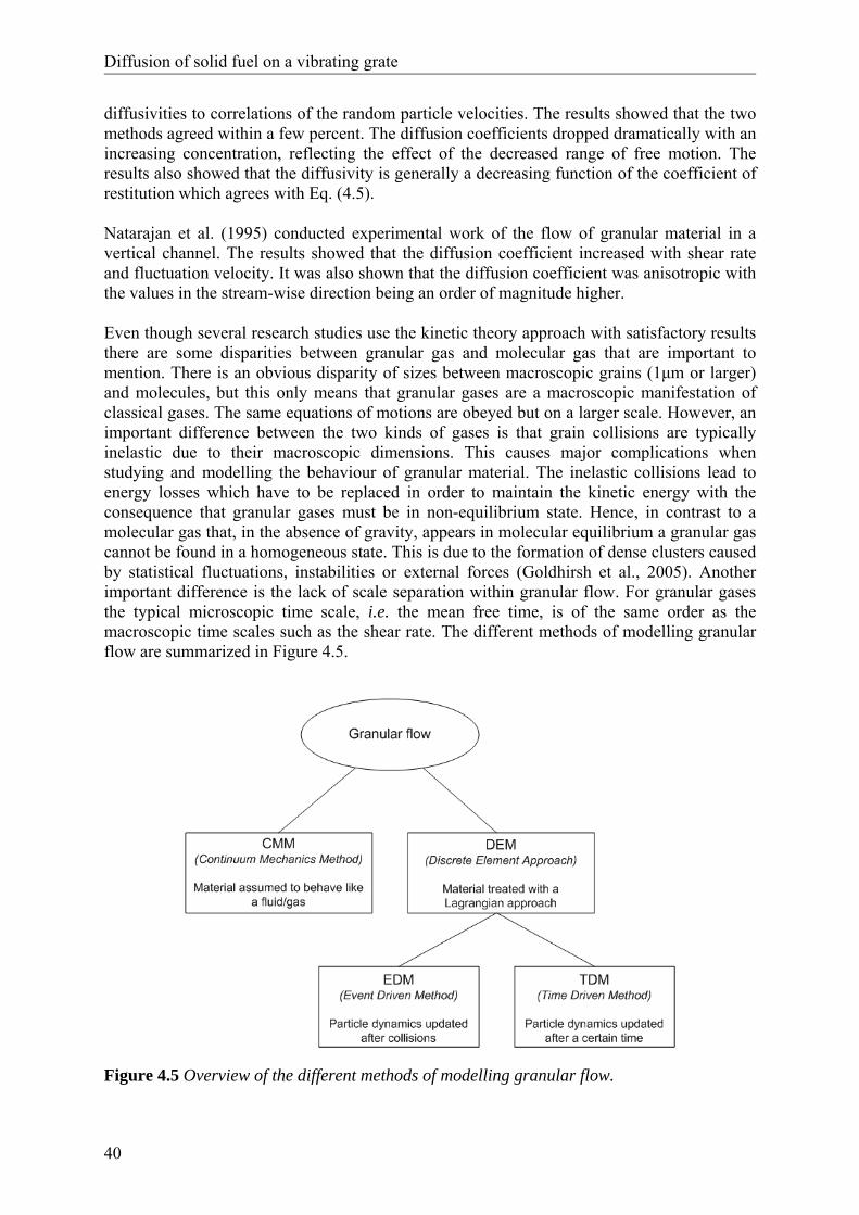
Diffusion of solid fuel on a vibrating grate
40
diffusivities to correlations of the random particle velocities. The results showed that the two methods agreed within a few percent. The diffusion coefficients dropped dramatically with an increasing concentration, reflecting the effect of the decreased range of free motion. The results also showed that the diffusivity is generally a decreasing function of the coefficient of restitution which agrees with Eq. (4.5). Natarajan et al. (1995) conducted experimental work of the flow of granular material in a vertical channel. The results showed that the diffusion coefficient increased with shear rate and fluctuation velocity. It was also shown that the diffusion coefficient was anisotropic with the values in the stream-wise direction being an order of magnitude higher. Even though several research studies use the kinetic theory approach with satisfactory results there are some disparities between granular gas and molecular gas that are important to mention. There is an obvious disparity of sizes between macroscopic grains (1μm or larger) and molecules, but this only means that granular gases are a macroscopic manifestation of classical gases. The same equations of motions are obeyed but on a larger scale. However, an important difference between the two kinds of gases is that grain collisions are typically inelastic due to their macroscopic dimensions. This causes major complications when studying and modelling the behaviour of granular material. The inelastic collisions lead to energy losses which have to be replaced in order to maintain the kinetic energy with the consequence that granular gases must be in non-equilibrium state. Hence, in contrast to a molecular gas that, in the absence of gravity, appears in molecular equilibrium a granular gas cannot be found in a homogeneous state. This is due to the formation of dense clusters caused by statistical fluctuations, instabilities or external forces (Goldhirsh et al., 2005). Another important difference is the lack of scale separation within granular flow. For granular gases the typical microscopic time scale, i.e. the mean free time, is of the same order as the macroscopic time scales such as the shear rate. The different methods of modelling granular flow are summarized in Figure 4.5.
Figure 4.5 Overview of the different methods of modelling granular flow.
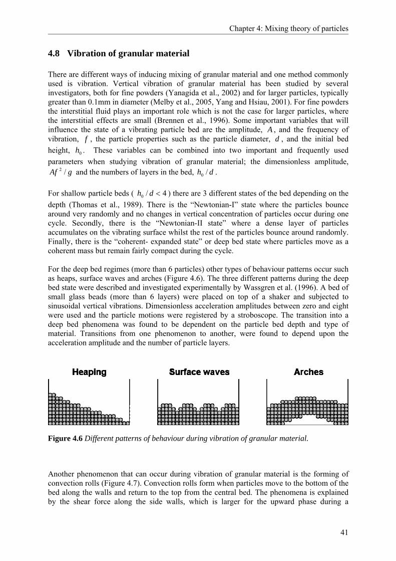
Chapter 4: Mixing theory of particles
41
4.8 Vibration of granular material There are different ways of inducing mixing of granular material and one method commonly used is vibration. Vertical vibration of granular material has been studied by several investigators, both for fine powders (Yanagida et al., 2002) and for larger particles, typically greater than 0.1mm in diameter (Melby et al., 2005, Yang and Hsiau, 2001). For fine powders the interstitial fluid plays an important role which is not the case for larger particles, where the interstitial effects are small (Brennen et al., 1996). Some important variables that will influence the state of a vibrating particle bed are the amplitude, A , and the frequency of vibration, f , the particle properties such as the particle diameter, d , and the initial bed height, 0h . These variables can be combined into two important and frequently used parameters when studying vibration of granular material; the dimensionless amplitude,
gAf /2 and the numbers of layers in the bed, dh /0 . For shallow particle beds ( 4/0 <dh ) there are 3 different states of the bed depending on the depth (Thomas et al., 1989). There is the “Newtonian-I” state where the particles bounce around very randomly and no changes in vertical concentration of particles occur during one cycle. Secondly, there is the “Newtonian-II state” where a dense layer of particles accumulates on the vibrating surface whilst the rest of the particles bounce around randomly. Finally, there is the “coherent- expanded state” or deep bed state where particles move as a coherent mass but remain fairly compact during the cycle. For the deep bed regimes (more than 6 particles) other types of behaviour patterns occur such as heaps, surface waves and arches (Figure 4.6). The three different patterns during the deep bed state were described and investigated experimentally by Wassgren et al. (1996). A bed of small glass beads (more than 6 layers) were placed on top of a shaker and subjected to sinusoidal vertical vibrations. Dimensionless acceleration amplitudes between zero and eight were used and the particle motions were registered by a stroboscope. The transition into a deep bed phenomena was found to be dependent on the particle bed depth and type of material. Transitions from one phenomenon to another, were found to depend upon the acceleration amplitude and the number of particle layers.
Figure 4.6 Different patterns of behaviour during vibration of granular material.
Another phenomenon that can occur during vibration of granular material is the forming of convection rolls (Figure 4.7). Convection rolls form when particles move to the bottom of the bed along the walls and return to the top from the central bed. The phenomena is explained by the shear force along the side walls, which is larger for the upward phase during a
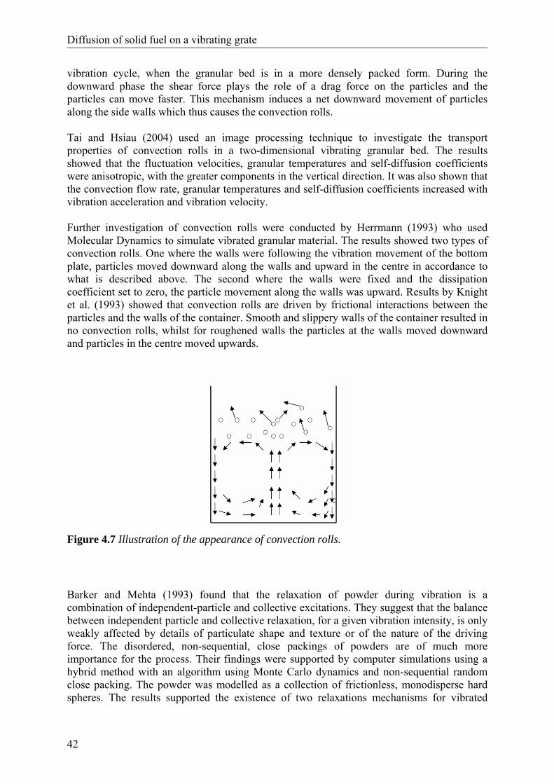
Diffusion of solid fuel on a vibrating grate
42
vibration cycle, when the granular bed is in a more densely packed form. During the downward phase the shear force plays the role of a drag force on the particles and the particles can move faster. This mechanism induces a net downward movement of particles along the side walls which thus causes the convection rolls. Tai and Hsiau (2004) used an image processing technique to investigate the transport properties of convection rolls in a two-dimensional vibrating granular bed. The results showed that the fluctuation velocities, granular temperatures and self-diffusion coefficients were anisotropic, with the greater components in the vertical direction. It was also shown that the convection flow rate, granular temperatures and self-diffusion coefficients increased with vibration acceleration and vibration velocity. Further investigation of convection rolls were conducted by Herrmann (1993) who used Molecular Dynamics to simulate vibrated granular material. The results showed two types of convection rolls. One where the walls were following the vibration movement of the bottom plate, particles moved downward along the walls and upward in the centre in accordance to what is described above. The second where the walls were fixed and the dissipation coefficient set to zero, the particle movement along the walls was upward. Results by Knight et al. (1993) showed that convection rolls are driven by frictional interactions between the particles and the walls of the container. Smooth and slippery walls of the container resulted in no convection rolls, whilst for roughened walls the particles at the walls moved downward and particles in the centre moved upwards.
Figure 4.7 Illustration of the appearance of convection rolls.
Barker and Mehta (1993) found that the relaxation of powder during vibration is a combination of independent-particle and collective excitations. They suggest that the balance between independent particle and collective relaxation, for a given vibration intensity, is only weakly affected by details of particulate shape and texture or of the nature of the driving force. The disordered, non-sequential, close packings of powders are of much more importance for the process. Their findings were supported by computer simulations using a hybrid method with an algorithm using Monte Carlo dynamics and non-sequential random close packing. The powder was modelled as a collection of frictionless, monodisperse hard spheres. The results supported the existence of two relaxations mechanisms for vibrated
Chapter 4: Mixing theory of particles
43
powders, a slower one that involved collective particle motions and a faster one that involved the motions of individual particles. Brennen et al. (1996) investigated the behaviour of a bed of granular material of large particles (2.85 mm diameter) subjected to vertical vibration. The important parameters were found to be: vibration frequency, vibration amplitude, particle diameter and bed height at rest as well as material properties such as coefficient of restitution for collisions between the individual particles and the base plate. In the range of frequencies explored (5-100 Hz) the mixing was relatively independent of the frequency but strongly dependent on the acceleration level and on the bed height. A simplification in computer simulations is that the particle reorganisation, caused by shaking, are only subject to geometrical constraints. However, for real powders the circumstances are more complicated, where forces, like cohesive forces and particle fragmentations, also contribute to the structural collapse during vibration. In the dynamic regime, where the particles move independently, the particles lose information concerning their relative positions. This loss of information induced by the shaking can be considered as a diffusive process (Barker and Metha, 1993). The positions of a particle, measured at the same phase point of consecutive shake cycles, will be slightly displaced, and it can be seen that a sequence of the finite displacements forms a three-dimensional random walk that represents the diffusive motion of particle due to shaking. The diffusive motion of a particle, in the direction of shaking, will always be greater than that in the other two orthogonal directions. To explain the reason for the diffusive motions is not straight forward. During each shaking cycle the particles are affected by a direct fluctuating force that arises from effective collisions between pairs of moving particles. However, the particles are also subjected to motions like rolling and falling, which results in other fluctuating forces. Thus, the random displacements of the particles are a result from a combination of different fluctuating processes depending on the vibration intensity. More investigation of self-diffusive behaviour in a vibrated bed was conducted by Yang and Hsiau (2001). Experimental and simulation methods were used to examine the effect of control parameters like dimensionless acceleration, vibration amplitude, vibration frequency, restitution coefficient and solid fraction on the diffusion coefficient. Experiments were carried out with glass beads (3mm diameter) placed in a vertical shaker. A camera captured the motion and auto correlation was used to analyse the particle movements. The behaviour was simulated by a Discrete Element Method (DEM). The fluctuation velocity and granular temperature were shown to be highly anisotropic, with a greater component in the vertical direction. The higher fluctuation velocities resulted in greater granular temperature and hence greater diffusion coefficient. The diffusion coefficients increased with the dimensionless acceleration amplitude. It was also strongly dependent on vibration bed velocity and very sensitive to the solid fraction. Hunt et al. (1994) carried out experiments to investigate how the mixing process depends on the vibration acceleration, frequency and bed height. A vertical shaker was used and the vibrated particles were red and blue spherical balls with a diameter of 3 mm placed in two different equally thick layers. The results showed that the expansion of the bed increased significantly beyond a critical frequency (10 Hz) and that the expansion did not depend on the amplitude of the vibrations. The solid fraction in the bed decreased with distance from the base plate. A mixing time was defined as the time it took for the particles from the layer underneath to move up to the upper layer so that an equal concentration of both colours were
Diffusion of solid fuel on a vibrating grate
44
represented in this layer. The mixing times decreased significantly when the bed reached an expanded state and a deeper bed resulted in a longer mixing time. Mixing time was also calculated theoretically with the diffusion equation and a theoretically calculated diffusion coefficient based on Eq. (4.5). The calculated values over predicted the experimental results which implies that the diffusion coefficient was under-estimated.
4.9 Mixing in bed models As mentioned previously the mixing process in bed models has not achieved much attention. The bed models are often treated under fixed bed conditions (e.g. van der Lans et al., 2000) or as a serial cascade of continuous stirred reactors (Beckmann and Scholtz, 1995). In the latter case, a mathematical model with the assumption that one of the stirred reactor elements moves along the length of the grate was developed. The mixing of the solid material due to the grate movement is expressed by integral expressions of temperature and oxygen concentration. Peters and Džiugys (2002) have used a DEM method to simulate the transport of fuel particles in combustion devices such as in rotary kilns or on travelling grates. A TDM is used and the dynamics of each particle are determined by the forces and torques acting on a particle. The bed is regarded as a finite number of particles with a given shape and visco-elastic material properties. Another approach, based on the kinetic theory, has been made by Lim et al (2001). They made experimental work with the purpose of characterizing and quantifying the mixing of waste on a travelling grate, so that the mixing process could be incorporated into a numerical bed model. Series of systematic particle tracking experiments were performed on scaled models of the three most commonly used industrial grates; the Deutsche Babcock Roller grate, the Martin Reverse Acting grate and the ABB Widmer and Ernst Motion Overthrust grate. The experiments showed that the tracers travel progressively down the grate with the rolling motion. A mathematical model was developed to simulate the movement of the solid material on the grate based on the probability for a solid tracer to swap position with the adjacent tracer. The process is essentially a random walk procedure and the numerical procedure is analogous to a discrete stochastic model called the Markov chain. Standard deviation, ( )s t , and mean values of the particle motion were calculated as function of time. The diffusion coefficient was then defined as:
2( )
2s tD
t= (4.7)
The mixing was included in a two-dimensional bed model for waste incineration, FLIC (Yang et al., 2002). Only the transverse (y) direction was studied and those calculations agreed well with the experimental results. The values of the diffusion coefficient varied between 0.03cm2/min and 3.60cm2/min. The experiments were later complemented with full scale tests for calculating the diffusion coefficients (Yang et al., 2005c). Tracer particles were introduced together with the waste into the incinerator. The exiting sequence and distribution across the grate were monitored through a sight glass at the end of the grate. Axial mixing was based on the particles residence time on the grate. Mean and standard deviation of the residence time were calculated and used to derive the diffusion coefficient. The axial diffusion coefficient xD , was found to vary between 27cm2/min and 109cm2/min. The vertical diffusion coefficient was assumed to be the same as the axial, since the combustion
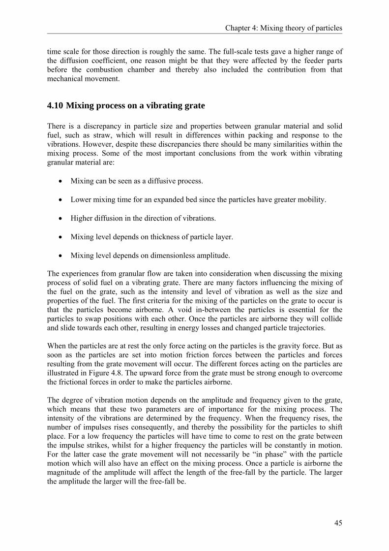
Chapter 4: Mixing theory of particles
45
time scale for those direction is roughly the same. The full-scale tests gave a higher range of the diffusion coefficient, one reason might be that they were affected by the feeder parts before the combustion chamber and thereby also included the contribution from that mechanical movement.
4.10 Mixing process on a vibrating grate There is a discrepancy in particle size and properties between granular material and solid fuel, such as straw, which will result in differences within packing and response to the vibrations. However, despite these discrepancies there should be many similarities within the mixing process. Some of the most important conclusions from the work within vibrating granular material are:
• Mixing can be seen as a diffusive process. • Lower mixing time for an expanded bed since the particles have greater mobility.
• Higher diffusion in the direction of vibrations.
• Mixing level depends on thickness of particle layer.
• Mixing level depends on dimensionless amplitude.
The experiences from granular flow are taken into consideration when discussing the mixing process of solid fuel on a vibrating grate. There are many factors influencing the mixing of the fuel on the grate, such as the intensity and level of vibration as well as the size and properties of the fuel. The first criteria for the mixing of the particles on the grate to occur is that the particles become airborne. A void in-between the particles is essential for the particles to swap positions with each other. Once the particles are airborne they will collide and slide towards each other, resulting in energy losses and changed particle trajectories. When the particles are at rest the only force acting on the particles is the gravity force. But as soon as the particles are set into motion friction forces between the particles and forces resulting from the grate movement will occur. The different forces acting on the particles are illustrated in Figure 4.8. The upward force from the grate must be strong enough to overcome the frictional forces in order to make the particles airborne. The degree of vibration motion depends on the amplitude and frequency given to the grate, which means that these two parameters are of importance for the mixing process. The intensity of the vibrations are determined by the frequency. When the frequency rises, the number of impulses rises consequently, and thereby the possibility for the particles to shift place. For a low frequency the particles will have time to come to rest on the grate between the impulse strikes, whilst for a higher frequency the particles will be constantly in motion. For the latter case the grate movement will not necessarily be “in phase” with the particle motion which will also have an effect on the mixing process. Once a particle is airborne the magnitude of the amplitude will affect the length of the free-fall by the particle. The larger the amplitude the larger will the free-fall be.
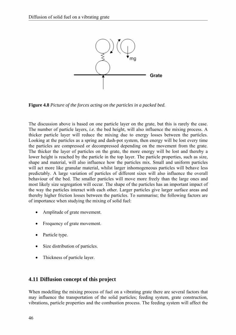
Diffusion of solid fuel on a vibrating grate
46
Figure 4.8 Picture of the forces acting on the particles in a packed bed. The discussion above is based on one particle layer on the grate, but this is rarely the case. The number of particle layers, i.e. the bed height, will also influence the mixing process. A thicker particle layer will reduce the mixing due to energy losses between the particles. Looking at the particles as a spring and dash-pot system, then energy will be lost every time the particles are compressed or decompressed depending on the movement from the grate. The thicker the layer of particles on the grate, the more energy will be lost and thereby a lower height is reached by the particle in the top layer. The particle properties, such as size, shape and material, will also influence how the particles mix. Small and uniform particles will act more like granular material, whilst larger inhomogeneous particles will behave less predictably. A large variation of particles of different sizes will also influence the overall behaviour of the bed. The smaller particles will move more freely than the large ones and most likely size segregation will occur. The shape of the particles has an important impact of the way the particles interact with each other. Larger particles give larger surface areas and thereby higher friction losses between the particles. To summarise; the following factors are of importance when studying the mixing of solid fuel:
• Amplitude of grate movement. • Frequency of grate movement. • Particle type. • Size distribution of particles.
• Thickness of particle layer.
4.11 Diffusion concept of this project When modelling the mixing process of fuel on a vibrating grate there are several factors that may influence the transportation of the solid particles; feeding system, grate construction, vibrations, particle properties and the combustion process. The feeding system will affect the
Chapter 4: Mixing theory of particles
47
initial velocity of the fuel and the amount of fuel on the grate which will determine the initial bed height. The properties of the fuel such as size, shape and bulk density will affect the particle-particle interactions and the interactions particle-grate. Also, the combustion process will affect the mixing process. During combustion the particles are going to change size and properties in the transition from raw fuel to ash. But the main reason for mixing will be the effect of the vibration of the grate. The level of vibration and the vibration sequences are most likely to play a key role in the mixing process. When looking at fuel transportation, there will be a mean movement of the fuel along the grate towards the ash pit. This can be seen as a convective transport, represented by the convective term in the transport equation. But, the vibrations will also give rise to a random mixing of the fuel on the grate. This random mixing can be compared to the diffusion process taking place in a molecular gas. If dividing a small section of the grate into two sides (A and B) and studying the transportation of particles of two different colours (e.g. black and white) across the interface some theoretical discussions can be made. Assuming an initial concentration difference of the particles in respective section, let us say that the concentration of black particles is twice as high on side A compared to side B (Figure 4.9), then the probability that a black particle will move from side A to B will be twice as high as the probability that a black particle will move from side B to A. Thus the probability of what particle that will move to the other side will depend on the concentration difference.
Figure 4.9 Illustration of the diffusion idea of this project.
As long as there exists a high concentration and low concentration region there will be a concentration gradient between the regions and the net flux will be from the high concentration region to the low concentration region. In this respect the process can be compared to a molecular gas and modelled by using the transport equation. Even if the driving mechanisms of the mixing are different for the two cases, the consequences will be similar. However, the diffusion coefficient for a vibrating grate will differ significantly from the one for a molecular gas. The value will most likely depend on the vibrations of the grate and also by the other parameters discussed previously. How a theoretical value of the diffusion coefficient should be derived is not straight-forward. One alternative is to experimentally derive the diffusion coefficient for a specific case.
Diffusion of solid fuel on a vibrating grate
48
In the next chapter, experimental work with the purpose of examining the diffusion coefficient for different grate constructions is presented. The particle trajectories are tracked so that the mixing process can be quantified. The diffusion coefficient is used in the above mentioned transport equation to numerically model the mixing of the fuel on the grate. The mean velocity on the grate is used as convective term. The magnitude of the velocity depends on the feeding velocity and the angle of the grate. A more tilted grate gives a higher horizontal velocity. The diffusion coefficient is calculated with help from the standard deviation of the particle velocities, i.e. the deviation from the mean velocity represents the random mixing. Similar to Eq. (4.5) the expression for the diffusion coefficient D , in this model looks like:
2
2sDt
= (4.8)
where s is the standard deviation of the particles trajectories during the time t . When developing mathematical models there is often a compromise involved between the modelling assumptions and the reality. If no vibration would take place the fuel bed would remain at rest and the combustion would take place under fixed bed assumptions. However, in order to obtain an efficient continuous combustion, the mixing of the fuel is essential and in order to develop an accurate bed model the understanding of the mixing process is of great importance.
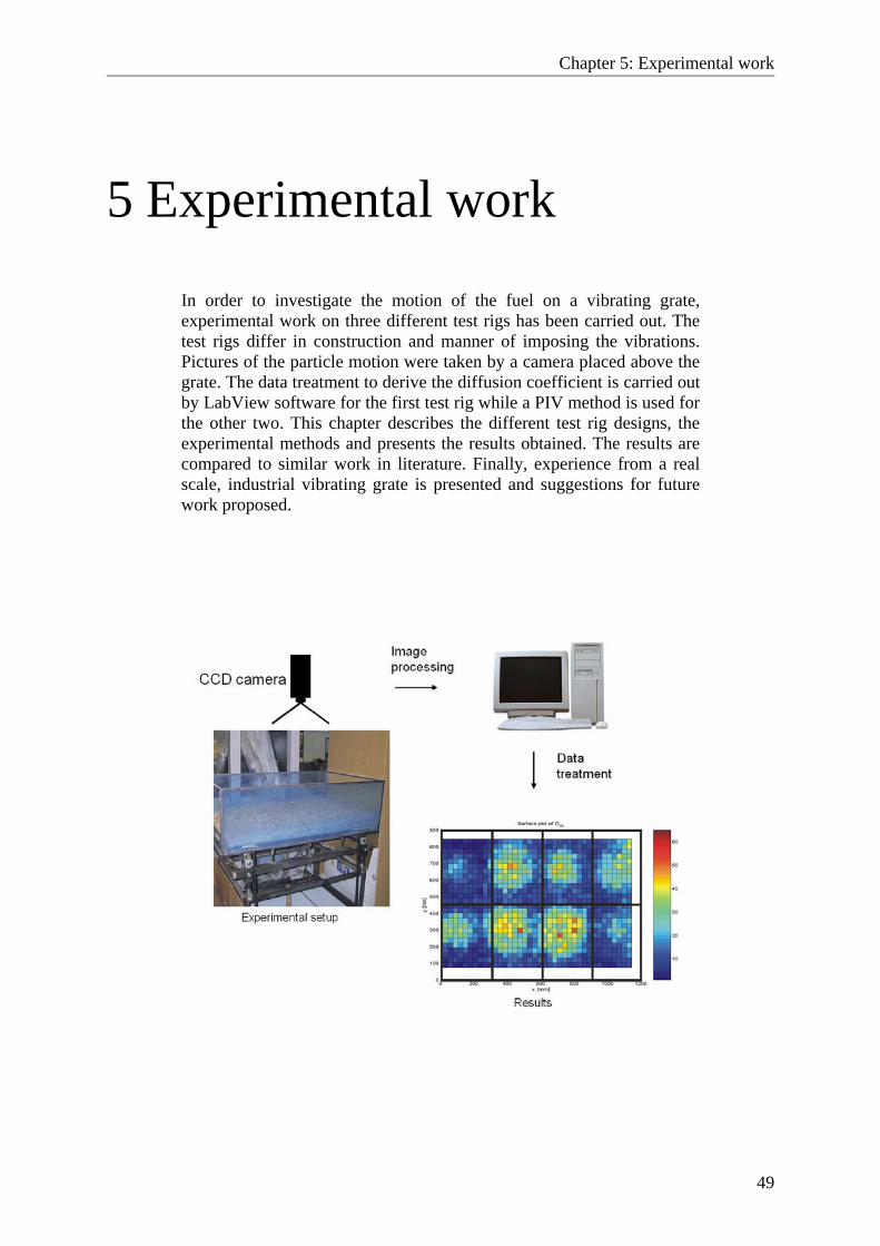
Chapter 5: Experimental work
49
5 Experimental work
In order to investigate the motion of the fuel on a vibrating grate, experimental work on three different test rigs has been carried out. The test rigs differ in construction and manner of imposing the vibrations. Pictures of the particle motion were taken by a camera placed above the grate. The data treatment to derive the diffusion coefficient is carried out by LabView software for the first test rig while a PIV method is used for the other two. This chapter describes the different test rig designs, the experimental methods and presents the results obtained. The results are compared to similar work in literature. Finally, experience from a real scale, industrial vibrating grate is presented and suggestions for future work proposed.
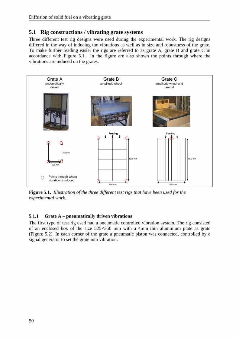
Diffusion of solid fuel on a vibrating grate
50
5.1 Rig constructions / vibrating grate systems Three different test rig designs were used during the experimental work. The rig designs differed in the way of inducing the vibrations as well as in size and robustness of the grate. To make further reading easier the rigs are referred to as grate A, grate B and grate C in accordance with Figure 5.1. In the figure are also shown the points through where the vibrations are induced on the grates.
Grate A pneumatically
driven
Grate B amplitude wheel
Grate Camplitude wheel and
ramrod
FeedingFeedingFeeding
1200 mm
800 mm
Feeding
1200 mm
800 mm
525 mm
350 mm
Points through where vibration is induced
Figure 5.1. Illustration of the three different test rigs that have been used for the experimental work.
5.1.1 Grate A – pneumatically driven vibrations The first type of test rig used had a pneumatic controlled vibration system. The rig consisted of an enclosed box of the size 525×350 mm with a 4mm thin aluminium plate as grate (Figure 5.2). In each corner of the grate a pneumatic piston was connected, controlled by a signal generator to set the grate into vibration.
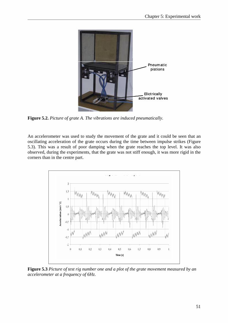
Chapter 5: Experimental work
51
Elictricallyactivated valves
Pneumaticpistions
Elictricallyactivated valves
Pneumaticpistions
Figure 5.2. Picture of grate A. The vibrations are induced pneumatically.
An accelerometer was used to study the movement of the grate and it could be seen that an oscillating acceleration of the grate occurs during the time between impulse strikes (Figure 5.3). This was a result of poor damping when the grate reaches the top level. It was also observed, during the experiments, that the grate was not stiff enough, it was more rigid in the corners than in the centre part.
Figure 5.3 Picture of test rig number one and a plot of the grate movement measured by an accelerometer at a frequency of 6Hz.
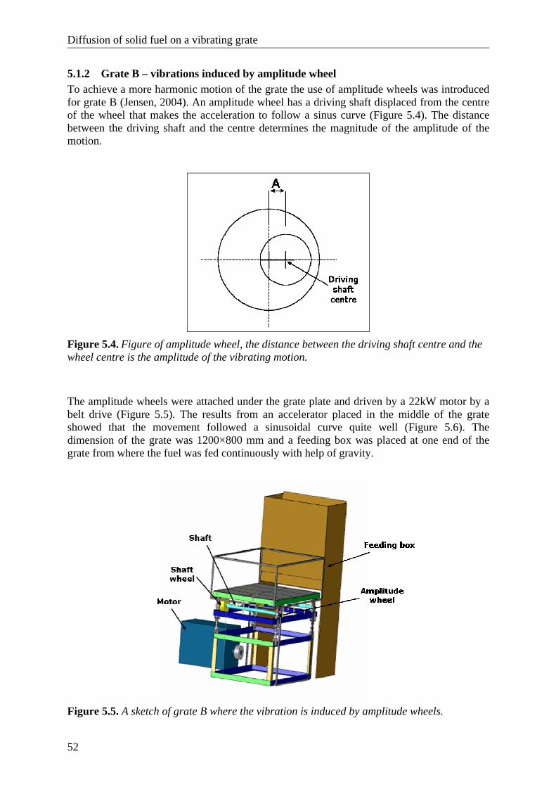
Diffusion of solid fuel on a vibrating grate
52
5.1.2 Grate B – vibrations induced by amplitude wheel To achieve a more harmonic motion of the grate the use of amplitude wheels was introduced for grate B (Jensen, 2004). An amplitude wheel has a driving shaft displaced from the centre of the wheel that makes the acceleration to follow a sinus curve (Figure 5.4). The distance between the driving shaft and the centre determines the magnitude of the amplitude of the motion.
Figure 5.4. Figure of amplitude wheel, the distance between the driving shaft centre and the wheel centre is the amplitude of the vibrating motion.
The amplitude wheels were attached under the grate plate and driven by a 22kW motor by a belt drive (Figure 5.5). The results from an accelerator placed in the middle of the grate showed that the movement followed a sinusoidal curve quite well (Figure 5.6). The dimension of the grate was 1200×800 mm and a feeding box was placed at one end of the grate from where the fuel was fed continuously with help of gravity.
Figure 5.5. A sketch of grate B where the vibration is induced by amplitude wheels.
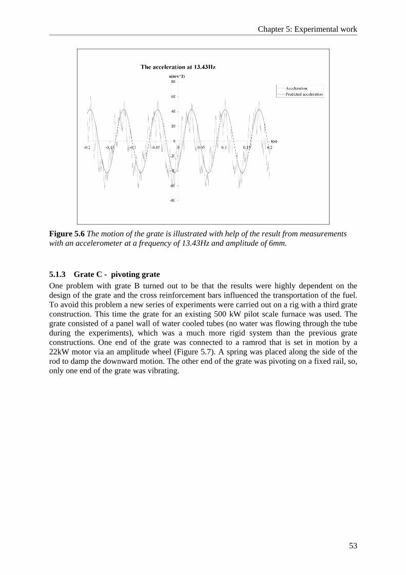
Chapter 5: Experimental work
53
Figure 5.6 The motion of the grate is illustrated with help of the result from measurements with an accelerometer at a frequency of 13.43Hz and amplitude of 6mm.
5.1.3 Grate C - pivoting grate One problem with grate B turned out to be that the results were highly dependent on the design of the grate and the cross reinforcement bars influenced the transportation of the fuel. To avoid this problem a new series of experiments were carried out on a rig with a third grate construction. This time the grate for an existing 500 kW pilot scale furnace was used. The grate consisted of a panel wall of water cooled tubes (no water was flowing through the tube during the experiments), which was a much more rigid system than the previous grate constructions. One end of the grate was connected to a ramrod that is set in motion by a 22kW motor via an amplitude wheel (Figure 5.7). A spring was placed along the side of the rod to damp the downward motion. The other end of the grate was pivoting on a fixed rail, so, only one end of the grate was vibrating.
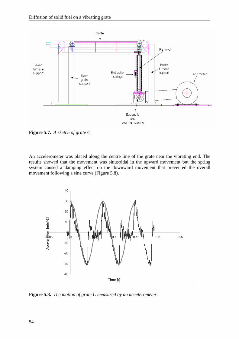
Diffusion of solid fuel on a vibrating grate
54
Figure 5.7. A sketch of grate C.
An accelerometer was placed along the centre line of the grate near the vibrating end. The results showed that the movement was sinusoidal in the upward movement but the spring system caused a damping effect on the downward movement that prevented the overall movement following a sine curve (Figure 5.8).
-40
-30
-20
-10
0
10
20
30
40
-0.05 0 0.05 0.1 0.15 0.2 0.25
Time [s]
Acce
lera
tion
[m/s
^2]
Figure 5.8. The motion of grate C measured by an accelerometer.
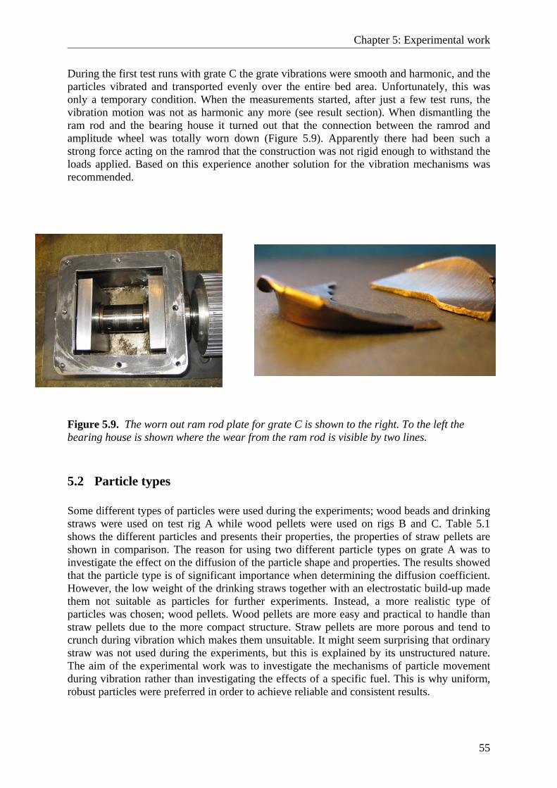
Chapter 5: Experimental work
55
During the first test runs with grate C the grate vibrations were smooth and harmonic, and the particles vibrated and transported evenly over the entire bed area. Unfortunately, this was only a temporary condition. When the measurements started, after just a few test runs, the vibration motion was not as harmonic any more (see result section). When dismantling the ram rod and the bearing house it turned out that the connection between the ramrod and amplitude wheel was totally worn down (Figure 5.9). Apparently there had been such a strong force acting on the ramrod that the construction was not rigid enough to withstand the loads applied. Based on this experience another solution for the vibration mechanisms was recommended.
Figure 5.9. The worn out ram rod plate for grate C is shown to the right. To the left the bearing house is shown where the wear from the ram rod is visible by two lines.
5.2 Particle types Some different types of particles were used during the experiments; wood beads and drinking straws were used on test rig A while wood pellets were used on rigs B and C. Table 5.1 shows the different particles and presents their properties, the properties of straw pellets are shown in comparison. The reason for using two different particle types on grate A was to investigate the effect on the diffusion of the particle shape and properties. The results showed that the particle type is of significant importance when determining the diffusion coefficient. However, the low weight of the drinking straws together with an electrostatic build-up made them not suitable as particles for further experiments. Instead, a more realistic type of particles was chosen; wood pellets. Wood pellets are more easy and practical to handle than straw pellets due to the more compact structure. Straw pellets are more porous and tend to crunch during vibration which makes them unsuitable. It might seem surprising that ordinary straw was not used during the experiments, but this is explained by its unstructured nature. The aim of the experimental work was to investigate the mechanisms of particle movement during vibration rather than investigating the effects of a specific fuel. This is why uniform, robust particles were preferred in order to achieve reliable and consistent results.
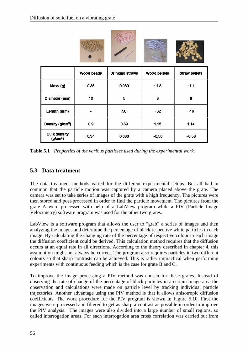
Diffusion of solid fuel on a vibrating grate
56
Table 5.1 Properties of the various particles used during the experimental work.
5.3 Data treatment The data treatment methods varied for the different experimental setups. But all had in common that the particle motion was captured by a camera placed above the grate. The camera was set to take series of images of the grate with a high frequency. The pictures were then stored and post-processed in order to find the particle movement. The pictures from the grate A were processed with help of a LabView program while a PIV (Particle Image Velocimetry) software program was used for the other two grates. LabView is a software program that allows the user to “grab” a series of images and then analyzing the images and determine the percentage of black respective white particles in each image. By calculating the changing rate of the percentage of respective colour in each image the diffusion coefficient could be derived. This calculation method requires that the diffusion occurs at an equal rate in all directions. According to the theory described in chapter 4, this assumption might not always be correct. The program also requires particles in two different colours so that sharp contrasts can be achieved. This is rather impractical when performing experiments with continuous feeding which is the case for grate B and C. To improve the image processing a PIV method was chosen for these grates. Instead of observing the rate of change of the percentage of black particles in a certain image area the observation and calculations were made on particle level by tracking individual particle trajectories. Another advantage using the PIV method is that it allows anisotropic diffusion coefficients. The work procedure for the PIV program is shown in Figure 5.10. First the images were processed and filtered to get as sharp a contrast as possible in order to improve the PIV analysis. The images were also divided into a large number of small regions, so called interrogation areas. For each interrogation area cross correlation was carried out from
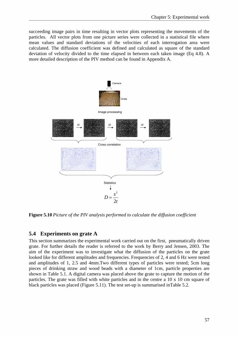
Chapter 5: Experimental work
57
succeeding image pairs in time resulting in vector plots representing the movements of the particles. All vector plots from one picture series were collected in a statistical file where mean values and standard deviations of the velocities of each interrogation area were calculated. The diffusion coefficient was defined and calculated as square of the standard deviation of velocity divided to the time elapsed in between each taken image (Eq 4.8). A more detailed description of the PIV method can be found in Appendix A.
Cross correlation
Statistics
Camera
Image processing
Grate
2
2sDt
=
∆t∆t ∆t
Figure 5.10 Picture of the PIV analysis performed to calculate the diffusion coefficient
5.4 Experiments on grate A This section summarizes the experimental work carried out on the first, pneumatically driven grate. For further details the reader is referred to the work by Berry and Jensen, 2003. The aim of the experiment was to investigate what the diffusion of the particles on the grate looked like for different amplitudes and frequencies. Frequencies of 2, 4 and 6 Hz were tested and amplitudes of 1, 2.5 and 4mm.Two different types of particles were tested; 5cm long pieces of drinking straw and wood beads with a diameter of 1cm, particle properties are shown in Table 5.1. A digital camera was placed above the grate to capture the motion of the particles. The grate was filled with white particles and in the centre a 10 x 10 cm square of black particles was placed (Figure 5.11). The test set-up is summarised inTable 5.2.
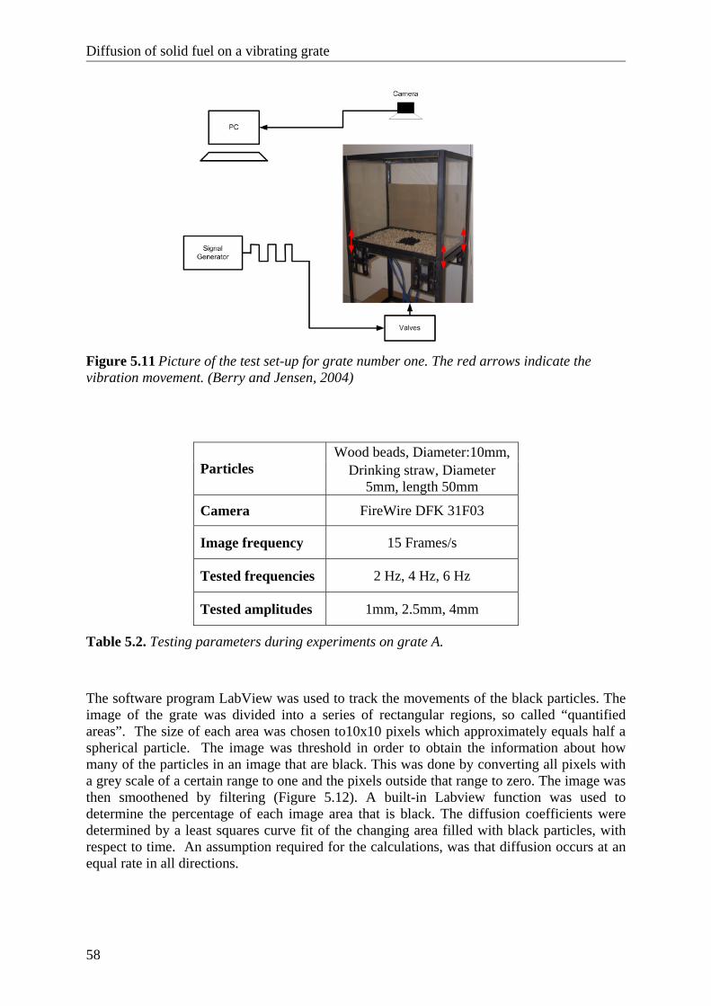
Diffusion of solid fuel on a vibrating grate
58
Figure 5.11 Picture of the test set-up for grate number one. The red arrows indicate the vibration movement. (Berry and Jensen, 2004)
Wood beads, Diameter:10mm, Particles Drinking straw, Diameter
5mm, length 50mm
Camera FireWire DFK 31F03
Image frequency 15 Frames/s
Tested frequencies 2 Hz, 4 Hz, 6 Hz
Tested amplitudes 1mm, 2.5mm, 4mm
Table 5.2. Testing parameters during experiments on grate A.
The software program LabView was used to track the movements of the black particles. The image of the grate was divided into a series of rectangular regions, so called “quantified areas”. The size of each area was chosen to10x10 pixels which approximately equals half a spherical particle. The image was threshold in order to obtain the information about how many of the particles in an image that are black. This was done by converting all pixels with a grey scale of a certain range to one and the pixels outside that range to zero. The image was then smoothened by filtering (Figure 5.12). A built-in Labview function was used to determine the percentage of each image area that is black. The diffusion coefficients were determined by a least squares curve fit of the changing area filled with black particles, with respect to time. An assumption required for the calculations, was that diffusion occurs at an equal rate in all directions.
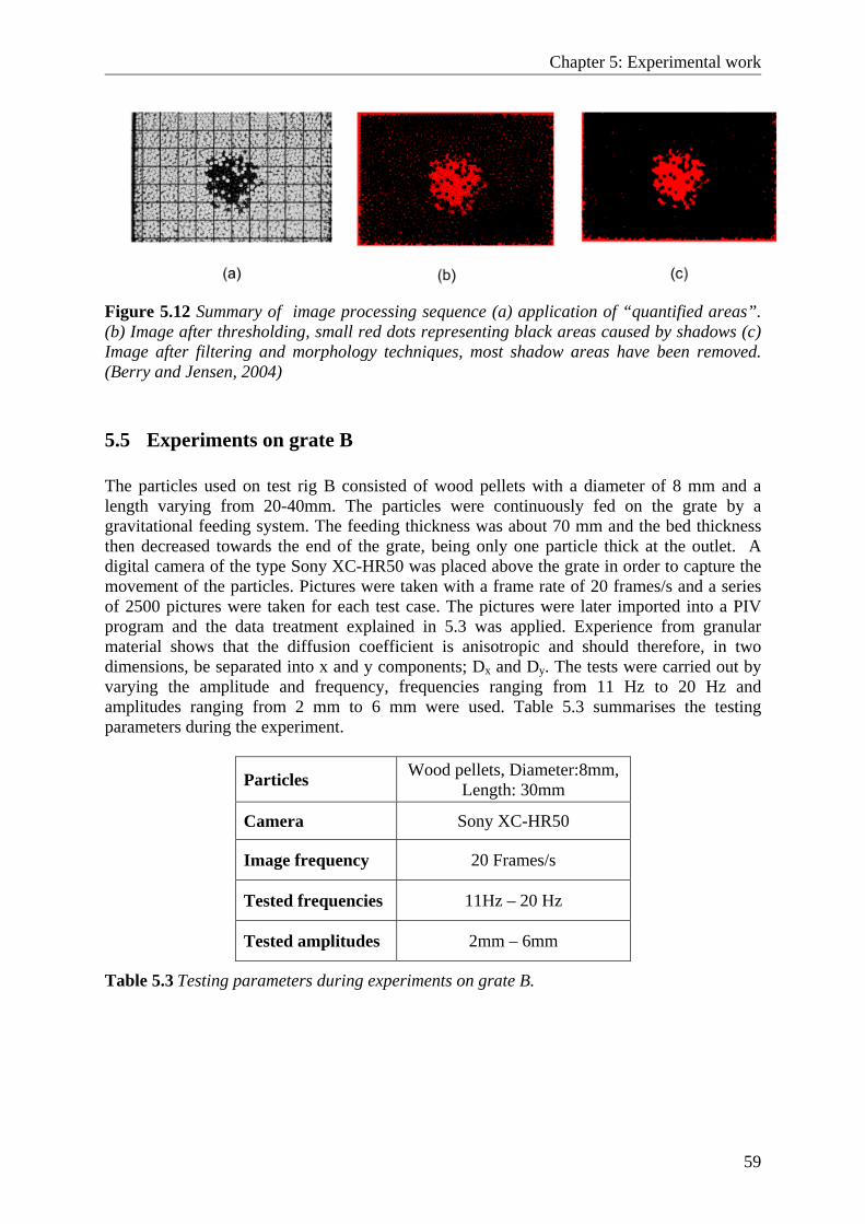
Chapter 5: Experimental work
59
Figure 5.12 Summary of image processing sequence (a) application of “quantified areas”. (b) Image after thresholding, small red dots representing black areas caused by shadows (c) Image after filtering and morphology techniques, most shadow areas have been removed. (Berry and Jensen, 2004)
5.5 Experiments on grate B The particles used on test rig B consisted of wood pellets with a diameter of 8 mm and a length varying from 20-40mm. The particles were continuously fed on the grate by a gravitational feeding system. The feeding thickness was about 70 mm and the bed thickness then decreased towards the end of the grate, being only one particle thick at the outlet. A digital camera of the type Sony XC-HR50 was placed above the grate in order to capture the movement of the particles. Pictures were taken with a frame rate of 20 frames/s and a series of 2500 pictures were taken for each test case. The pictures were later imported into a PIV program and the data treatment explained in 5.3 was applied. Experience from granular material shows that the diffusion coefficient is anisotropic and should therefore, in two dimensions, be separated into x and y components; Dx and Dy. The tests were carried out by varying the amplitude and frequency, frequencies ranging from 11 Hz to 20 Hz and amplitudes ranging from 2 mm to 6 mm were used. Table 5.3 summarises the testing parameters during the experiment.
Particles Wood pellets, Diameter:8mm, Length: 30mm
Camera Sony XC-HR50
Image frequency 20 Frames/s
Tested frequencies 11Hz – 20 Hz
Tested amplitudes 2mm – 6mm
Table 5.3 Testing parameters during experiments on grate B.
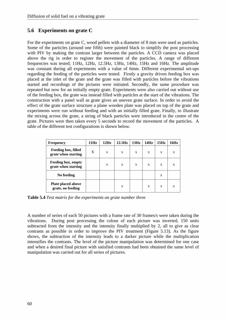
Diffusion of solid fuel on a vibrating grate
60
5.6 Experiments on grate C For the experiments on grate C, wood pellets with a diameter of 8 mm were used as particles. Some of the particles (around one fifth) were painted black to simplify the post processing with PIV by making the contrast larger between the particles. A CCD camera was placed above the rig in order to register the movement of the particles. A range of different frequencies was tested; 11Hz, 12Hz, 12.5Hz, 13Hz, 14Hz, 15Hz and 16Hz. The amplitude was constant during all experiments with a value of 6mm. Different experimental set-ups regarding the feeding of the particles were tested. Firstly a gravity driven feeding box was placed at the inlet of the grate and the grate was filled with particles before the vibrations started and recordings of the pictures were initiated. Secondly, the same procedure was repeated but now for an initially empty grate. Experiments were also carried out without use of the feeding box, the grate was instead filled with particles at the start of the vibrations. The construction with a panel wall as grate gives an uneven grate surface. In order to avoid the effect of the grate surface structure a plane wooden plate was placed on top of the grate and experiments were run without feeding and with an initially filled grate. Finally, to illustrate the mixing across the grate, a string of black particles were introduced in the centre of the grate. Pictures were then taken every 5 seconds to record the movement of the particles. A table of the different test configurations is shown below.
Frequency 11Hz 12Hz 12.5Hz 13Hz 14Hz 15Hz 16Hz
Feeding box, filled grate when starting X x x x x x x
Feeding box, empty grate when starting x x x x x x
No feeding x
Plate placed above grate, no feeding x x x x
Table 5.4 Test matrix for the experiments on grate number three
A number of series of each 50 pictures with a frame rate of 30 frames/s were taken during the vibrations. During post processing the colour of each picture was inverted, 150 units subtracted from the intensity and the intensity finally multiplied by 2, all to give as clear contrasts as possible in order to improve the PIV treatment (Figure 5.13). As the figure shows, the subtraction of the intensity leads to a darker picture while the multiplication intensifies the contrasts. The level of the picture manipulation was determined for one case and when a desired final picture with satisfied contrasts had been obtained the same level of manipulation was carried out for all series of pictures.
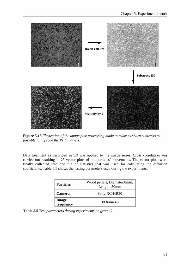
Chapter 5: Experimental work
61
Invert colours
Substract 150
Multiply by 2
Figure 5.13 Illustration of the image post processing made to make as sharp contrasts as possible to improve the PIV analysis.
Data treatment as described in 5.3 was applied to the image series. Cross correlation was carried out resulting in 25 vector plots of the particles’ movements. The vector plots were finally collected into one file of statistics that was used for calculating the diffusion coefficients. Table 5.5 shows the testing parameters used during the experiments.
Particles Wood pellets, Diameter:8mm, Length: 30mm
Camera Sony XC-HR50
Image frequency 30 frames/s
Table 5.5 Test parameters during experiments on grate C
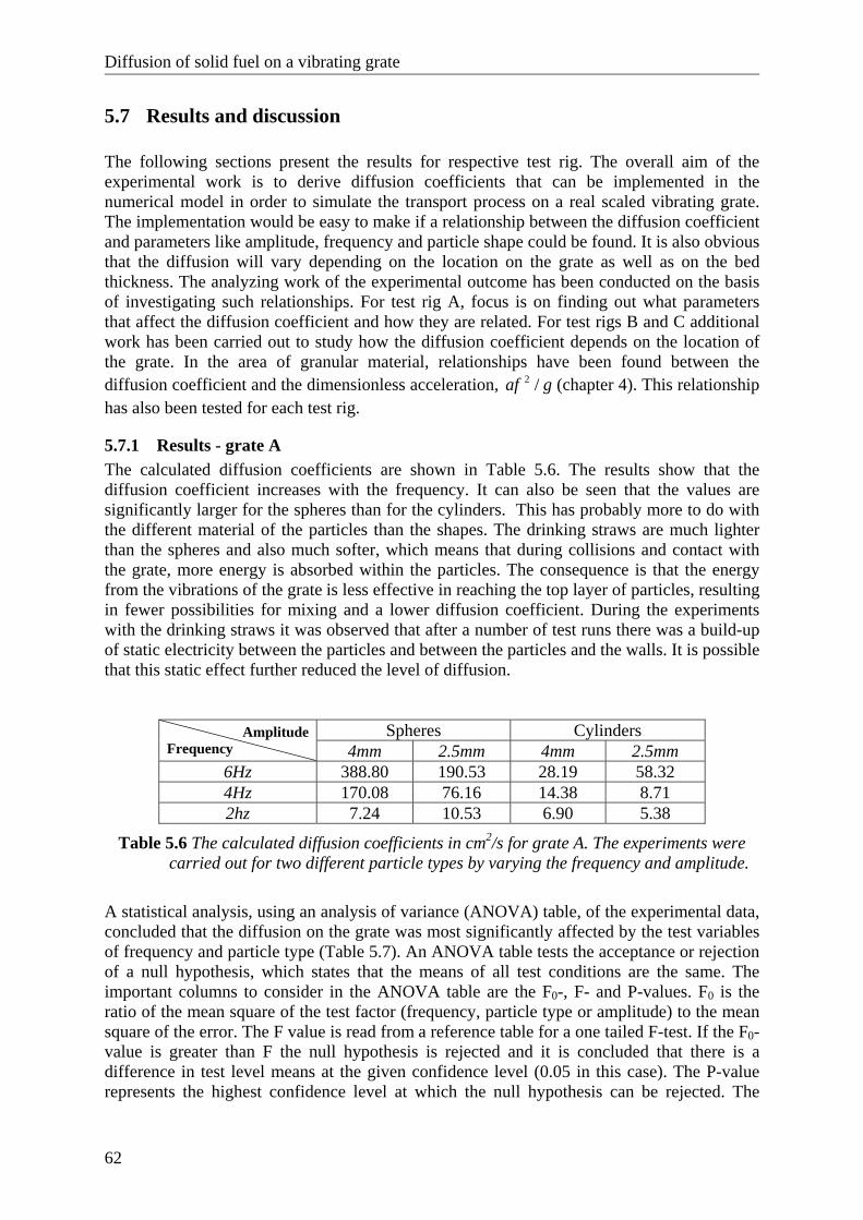
Diffusion of solid fuel on a vibrating grate
62
5.7 Results and discussion The following sections present the results for respective test rig. The overall aim of the experimental work is to derive diffusion coefficients that can be implemented in the numerical model in order to simulate the transport process on a real scaled vibrating grate. The implementation would be easy to make if a relationship between the diffusion coefficient and parameters like amplitude, frequency and particle shape could be found. It is also obvious that the diffusion will vary depending on the location on the grate as well as on the bed thickness. The analyzing work of the experimental outcome has been conducted on the basis of investigating such relationships. For test rig A, focus is on finding out what parameters that affect the diffusion coefficient and how they are related. For test rigs B and C additional work has been carried out to study how the diffusion coefficient depends on the location of the grate. In the area of granular material, relationships have been found between the diffusion coefficient and the dimensionless acceleration, gaf /2 (chapter 4). This relationship has also been tested for each test rig.
5.7.1 Results - grate A The calculated diffusion coefficients are shown in Table 5.6. The results show that the diffusion coefficient increases with the frequency. It can also be seen that the values are significantly larger for the spheres than for the cylinders. This has probably more to do with the different material of the particles than the shapes. The drinking straws are much lighter than the spheres and also much softer, which means that during collisions and contact with the grate, more energy is absorbed within the particles. The consequence is that the energy from the vibrations of the grate is less effective in reaching the top layer of particles, resulting in fewer possibilities for mixing and a lower diffusion coefficient. During the experiments with the drinking straws it was observed that after a number of test runs there was a build-up of static electricity between the particles and between the particles and the walls. It is possible that this static effect further reduced the level of diffusion.
Spheres Cylinders Amplitude Frequency 4mm 2.5mm 4mm 2.5mm
6Hz 388.80 190.53 28.19 58.32 4Hz 170.08 76.16 14.38 8.71 2hz 7.24 10.53 6.90 5.38
Table 5.6 The calculated diffusion coefficients in cm2/s for grate A. The experiments were carried out for two different particle types by varying the frequency and amplitude.
A statistical analysis, using an analysis of variance (ANOVA) table, of the experimental data, concluded that the diffusion on the grate was most significantly affected by the test variables of frequency and particle type (Table 5.7). An ANOVA table tests the acceptance or rejection of a null hypothesis, which states that the means of all test conditions are the same. The important columns to consider in the ANOVA table are the F0-, F- and P-values. F0 is the ratio of the mean square of the test factor (frequency, particle type or amplitude) to the mean square of the error. The F value is read from a reference table for a one tailed F-test. If the F0-value is greater than F the null hypothesis is rejected and it is concluded that there is a difference in test level means at the given confidence level (0.05 in this case). The P-value represents the highest confidence level at which the null hypothesis can be rejected. The
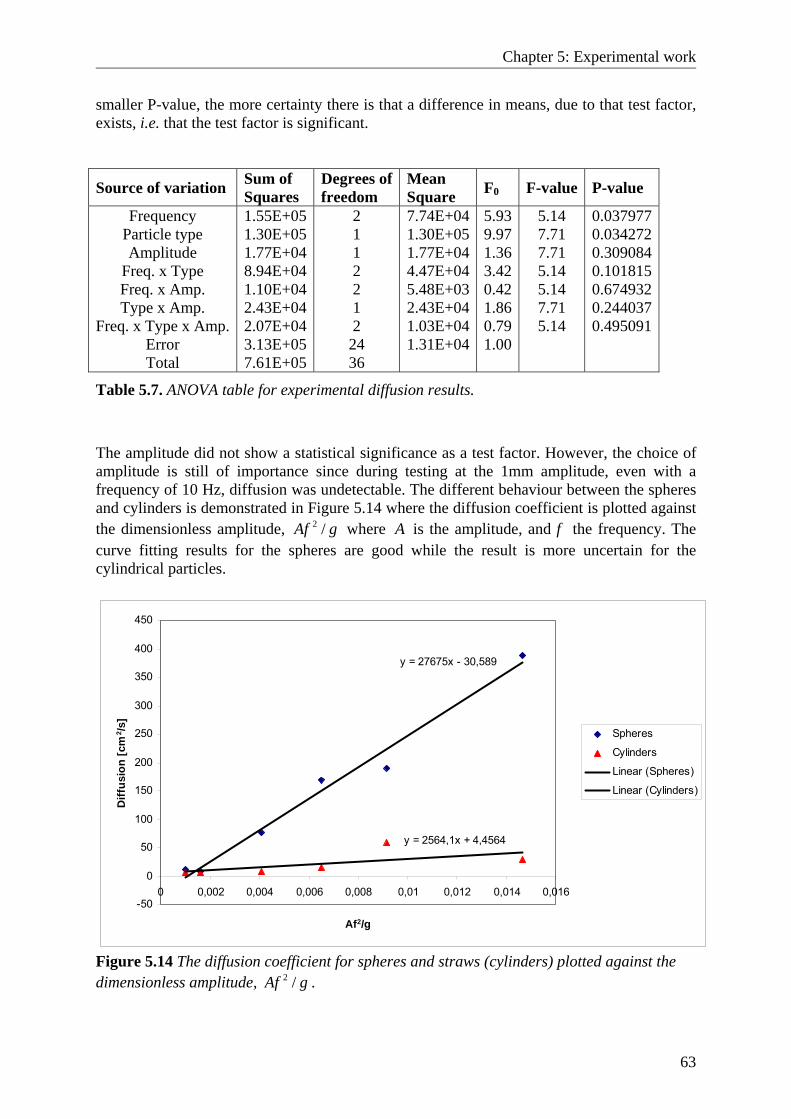
Chapter 5: Experimental work
63
smaller P-value, the more certainty there is that a difference in means, due to that test factor, exists, i.e. that the test factor is significant.
Source of variation Sum of Squares
Degrees of freedom
Mean Square F0 F-value P-value
Frequency Particle type Amplitude
Freq. x Type Freq. x Amp. Type x Amp.
Freq. x Type x Amp. Error Total
1.55E+05 1.30E+05 1.77E+04 8.94E+04 1.10E+04 2.43E+04 2.07E+04 3.13E+05 7.61E+05
2 1 1 2 2 1 2 24 36
7.74E+041.30E+051.77E+044.47E+045.48E+032.43E+041.03E+041.31E+04
5.939.971.363.420.421.860.791.00
5.14 7.71 7.71 5.14 5.14 7.71 5.14
0.037977 0.034272 0.309084 0.101815 0.674932 0.244037 0.495091
Table 5.7. ANOVA table for experimental diffusion results.
The amplitude did not show a statistical significance as a test factor. However, the choice of amplitude is still of importance since during testing at the 1mm amplitude, even with a frequency of 10 Hz, diffusion was undetectable. The different behaviour between the spheres and cylinders is demonstrated in Figure 5.14 where the diffusion coefficient is plotted against the dimensionless amplitude, 2 /Af g where A is the amplitude, and f the frequency. The curve fitting results for the spheres are good while the result is more uncertain for the cylindrical particles.
y = 27675x - 30,589
y = 2564,1x + 4,4564
-50
0
50
100
150
200
250
300
350
400
450
0 0,002 0,004 0,006 0,008 0,01 0,012 0,014 0,016
Af2/g
Diff
usio
n [c
m2 /s
]
Spheres
Cylinders
Linear (Spheres)
Linear (Cylinders)
Figure 5.14 The diffusion coefficient for spheres and straws (cylinders) plotted against the dimensionless amplitude, 2 /Af g .
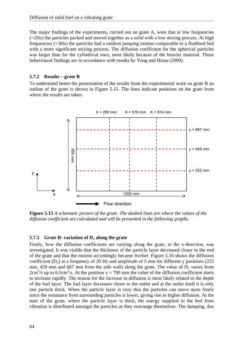
Diffusion of solid fuel on a vibrating grate
64
The major findings of the experiments, carried out on grate A, were that at low frequencies (<2Hz) the particles packed and moved together as a solid with a low mixing process. At high frequencies (>3Hz) the particles had a random jumping motion comparable to a fluidised bed with a more significant mixing process. The diffusion coefficient for the spherical particles was larger than for the cylindrical ones, most likely because of the heavier material. These behavioural findings are in accordance with results by Yang and Hsiau (2000).
5.7.2 Results – grate B To understand better the presentation of the results from the experimental work on grate B an outline of the grate is shown in Figure 5.15. The lines indicate positions on the grate from where the results are taken.
Figure 5.15 A schematic picture of the grate. The dashed lines are where the values of the diffusion coefficient are calculated and will be presented in the following graphs.
5.7.3 Grate B- variation of Dx along the grate Firstly, how the diffusion coefficients are varying along the grate, in the x-direction, was investigated. It was visible that the thickness of the particle layer decreased closer to the end of the grate and that the motion accordingly became livelier. Figure 5.16 shows the diffusion coefficient (Dx) at a frequency of 20 Hz and amplitude of 5 mm for different y positions (222 mm, 459 mm and 667 mm from the side wall) along the grate. The value of Dx varies from 2cm2/s up to 6.5cm2/s. At the position x = 700 mm the value of the diffusion coefficient starts to increase rapidly. The reason for the increase in diffusion is most likely related to the depth of the fuel layer. The fuel layer decreases closer to the outlet and at the outlet itself it is only one particle thick. When the particle layer is very thin the particles can move more freely since the resistance from surrounding particles is lower, giving rise to higher diffusion. At the start of the grate, where the particle layer is thick, the energy supplied to the bed from vibration is distributed amongst the particles as they rearrange themselves. The damping, due
y
x
y = 222 mm
y = 459 mm
y = 667 mm
X = 260 mm X = 578 mm X = 874 mm
Flow direction
1200 mm
800 mm
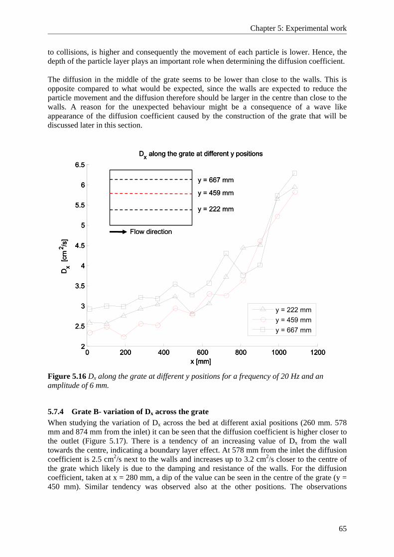
Chapter 5: Experimental work
65
to collisions, is higher and consequently the movement of each particle is lower. Hence, the depth of the particle layer plays an important role when determining the diffusion coefficient. The diffusion in the middle of the grate seems to be lower than close to the walls. This is opposite compared to what would be expected, since the walls are expected to reduce the particle movement and the diffusion therefore should be larger in the centre than close to the walls. A reason for the unexpected behaviour might be a consequence of a wave like appearance of the diffusion coefficient caused by the construction of the grate that will be discussed later in this section.
y = 222 mmy = 459 mmy = 667 mm
Flow direction
y = 222 mmy = 459 mmy = 667 mm
Flow direction
0 200 400 600 800 1000 12002
2.5
3
3.5
4
4.5
5
5.5
6
6.5Dx along the grate at different y positions
x [mm]
Dx
[cm
2 /s]
y = 222 mmy = 459 mmy = 667 mm
y = 222 mm
y = 459 mm
y = 667 mm
Flow direction
0 200 400 600 800 1000 12002
2.5
3
3.5
4
4.5
5
5.5
6
6.5Dx along the grate at different y positions
x [mm]
Dx
[cm
2 /s]
y = 222 mmy = 459 mmy = 667 mm
0 200 400 600 800 1000 12002
2.5
3
3.5
4
4.5
5
5.5
6
6.5Dx along the grate at different y positions
x [mm]
Dx
[cm
2 /s]
y = 222 mmy = 459 mmy = 667 mm
y = 222 mm
y = 459 mm
y = 667 mm
Flow direction
y = 222 mm
y = 459 mm
y = 667 mm
Flow direction
Figure 5.16 Dx along the grate at different y positions for a frequency of 20 Hz and an amplitude of 6 mm.
5.7.4 Grate B- variation of Dx across the grate When studying the variation of Dx across the bed at different axial positions (260 mm. 578 mm and 874 mm from the inlet) it can be seen that the diffusion coefficient is higher closer to the outlet (Figure 5.17). There is a tendency of an increasing value of Dx from the wall towards the centre, indicating a boundary layer effect. At 578 mm from the inlet the diffusion coefficient is 2.5 cm2/s next to the walls and increases up to 3.2 cm2/s closer to the centre of the grate which likely is due to the damping and resistance of the walls. For the diffusion coefficient, taken at x = 280 mm, a dip of the value can be seen in the centre of the grate (y = 450 mm). Similar tendency was observed also at the other positions. The observations
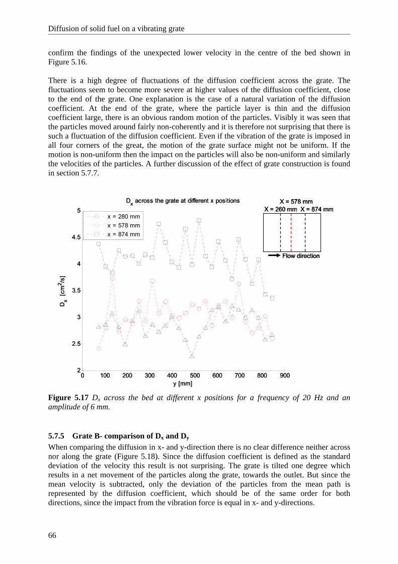
Diffusion of solid fuel on a vibrating grate
66
confirm the findings of the unexpected lower velocity in the centre of the bed shown in Figure 5.16. There is a high degree of fluctuations of the diffusion coefficient across the grate. The fluctuations seem to become more severe at higher values of the diffusion coefficient, close to the end of the grate. One explanation is the case of a natural variation of the diffusion coefficient. At the end of the grate, where the particle layer is thin and the diffusion coefficient large, there is an obvious random motion of the particles. Visibly it was seen that the particles moved around fairly non-coherently and it is therefore not surprising that there is such a fluctuation of the diffusion coefficient. Even if the vibration of the grate is imposed in all four corners of the great, the motion of the grate surface might not be uniform. If the motion is non-uniform then the impact on the particles will also be non-uniform and similarly the velocities of the particles. A further discussion of the effect of grate construction is found in section 5.7.7.
0 100 200 300 400 500 600 700 800 9002
2.5
3
3.5
4
4.5
5Dx across the grate at different x positions
y [mm]
Dx [
cm2 /s
]
x = 280 mmx = 578 mmx = 874 mm
X = 260 mmX = 578 mm
X = 874 mm
Flow direction
0 100 200 300 400 500 600 700 800 9002
2.5
3
3.5
4
4.5
5Dx across the grate at different x positions
y [mm]
Dx [
cm2 /s
]
x = 280 mmx = 578 mmx = 874 mm
X = 260 mmX = 578 mm
X = 874 mm
Flow direction
X = 260 mmX = 578 mm
X = 874 mm
Flow direction
Figure 5.17 Dx across the bed at different x positions for a frequency of 20 Hz and an amplitude of 6 mm.
5.7.5 Grate B- comparison of Dx and Dy When comparing the diffusion in x- and y-direction there is no clear difference neither across nor along the grate (Figure 5.18). Since the diffusion coefficient is defined as the standard deviation of the velocity this result is not surprising. The grate is tilted one degree which results in a net movement of the particles along the grate, towards the outlet. But since the mean velocity is subtracted, only the deviation of the particles from the mean path is represented by the diffusion coefficient, which should be of the same order for both directions, since the impact from the vibration force is equal in x- and y-directions.
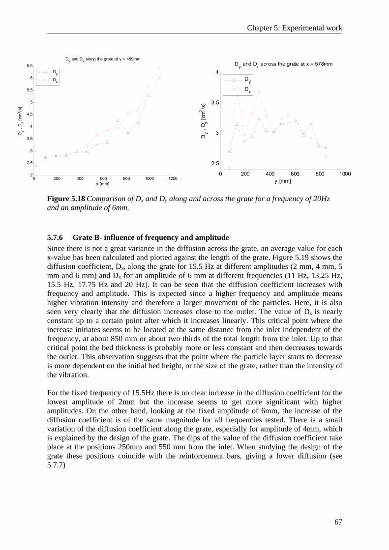
Chapter 5: Experimental work
67
0 200 400 600 800 1000 12002
2.5
3
3.5
4
4.5
5
5.5
6
6.5Dy and Dx along the grate at y = 459mm
x [mm]
Dy ,
Dx [c
m2 /s
]
Dy
Dx
0 200 400 600 800 1000
2.5
3
3.5
4Dy and Dx across the grate at x = 578mm
y [mm]
Dy ,
D x [cm
2 /s]
Dy
Dx
Figure 5.18 Comparison of Dx and Dy along and across the grate for a frequency of 20Hz and an amplitude of 6mm.
5.7.6 Grate B- influence of frequency and amplitude Since there is not a great variance in the diffusion across the grate, an average value for each x-value has been calculated and plotted against the length of the grate. Figure 5.19 shows the diffusion coefficient, Dx, along the grate for 15.5 Hz at different amplitudes (2 mm, 4 mm, 5 mm and 6 mm) and Dx for an amplitude of 6 mm at different frequencies (11 Hz, 13.25 Hz, 15.5 Hz, 17.75 Hz and 20 Hz). It can be seen that the diffusion coefficient increases with frequency and amplitude. This is expected since a higher frequency and amplitude means higher vibration intensity and therefore a larger movement of the particles. Here, it is also seen very clearly that the diffusion increases close to the outlet. The value of Dx is nearly constant up to a certain point after which it increases linearly. This critical point where the increase initiates seems to be located at the same distance from the inlet independent of the frequency, at about 850 mm or about two thirds of the total length from the inlet. Up to that critical point the bed thickness is probably more or less constant and then decreases towards the outlet. This observation suggests that the point where the particle layer starts to decrease is more dependent on the initial bed height, or the size of the grate, rather than the intensity of the vibration. For the fixed frequency of 15.5Hz there is no clear increase in the diffusion coefficient for the lowest amplitude of 2mm but the increase seems to get more significant with higher amplitudes. On the other hand, looking at the fixed amplitude of 6mm, the increase of the diffusion coefficient is of the same magnitude for all frequencies tested. There is a small variation of the diffusion coefficient along the grate, especially for amplitude of 4mm, which is explained by the design of the grate. The dips of the value of the diffusion coefficient take place at the positions 250mm and 550 mm from the inlet. When studying the design of the grate these positions coincide with the reinforcement bars, giving a lower diffusion (see 5.7.7)
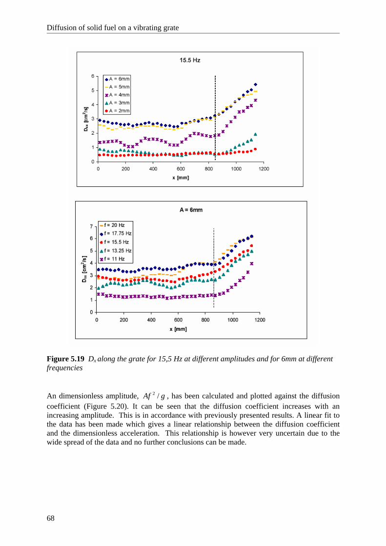
Diffusion of solid fuel on a vibrating grate
68
Figure 5.19 Dx along the grate for 15,5 Hz at different amplitudes and for 6mm at different frequencies An dimensionless amplitude, gAf /2 , has been calculated and plotted against the diffusion coefficient (Figure 5.20). It can be seen that the diffusion coefficient increases with an increasing amplitude. This is in accordance with previously presented results. A linear fit to the data has been made which gives a linear relationship between the diffusion coefficient and the dimensionless acceleration. This relationship is however very uncertain due to the wide spread of the data and no further conclusions can be made.
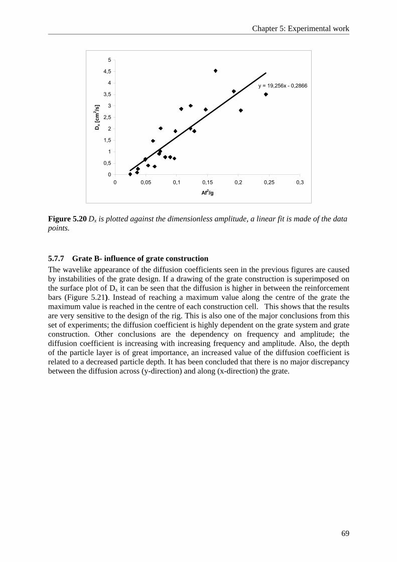
Chapter 5: Experimental work
69
y = 19,256x - 0,2866
0
0,5
1
1,5
2
2,5
3
3,5
4
4,5
5
0 0,05 0,1 0,15 0,2 0,25 0,3
Af2/g
Dx [
cm2 /s
]
Figure 5.20 Dx is plotted against the dimensionless amplitude, a linear fit is made of the data points.
5.7.7 Grate B- influence of grate construction The wavelike appearance of the diffusion coefficients seen in the previous figures are caused by instabilities of the grate design. If a drawing of the grate construction is superimposed on the surface plot of Dx it can be seen that the diffusion is higher in between the reinforcement bars (Figure 5.21). Instead of reaching a maximum value along the centre of the grate the maximum value is reached in the centre of each construction cell. This shows that the results are very sensitive to the design of the rig. This is also one of the major conclusions from this set of experiments; the diffusion coefficient is highly dependent on the grate system and grate construction. Other conclusions are the dependency on frequency and amplitude; the diffusion coefficient is increasing with increasing frequency and amplitude. Also, the depth of the particle layer is of great importance, an increased value of the diffusion coefficient is related to a decreased particle depth. It has been concluded that there is no major discrepancy between the diffusion across (y-direction) and along (x-direction) the grate.
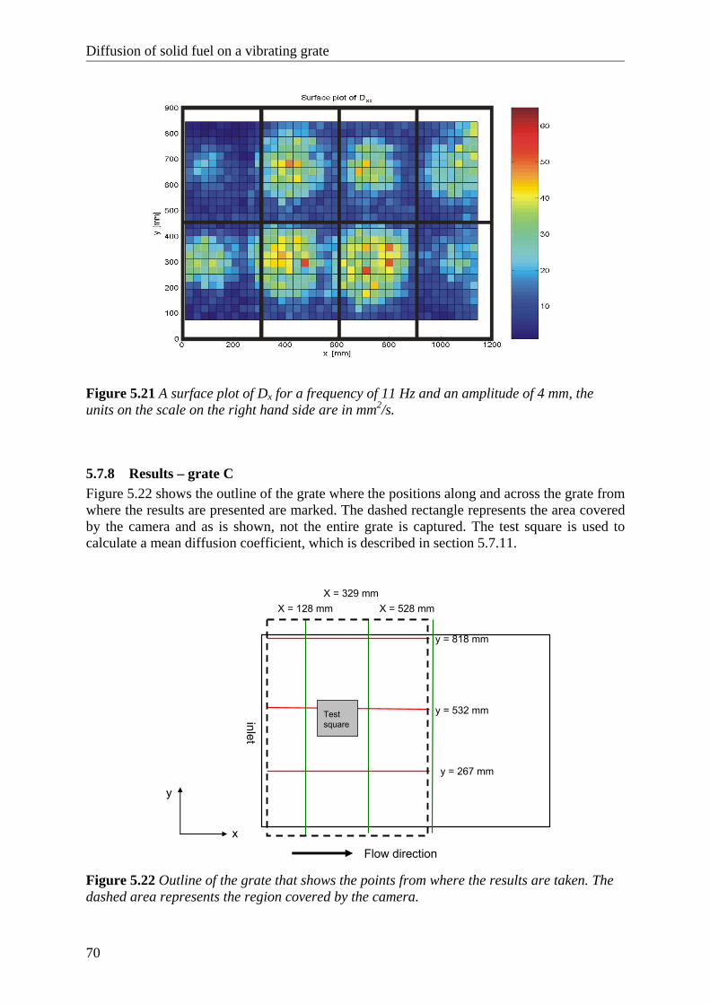
Diffusion of solid fuel on a vibrating grate
70
Figure 5.21 A surface plot of Dx for a frequency of 11 Hz and an amplitude of 4 mm, the units on the scale on the right hand side are in mm2/s.
5.7.8 Results – grate C Figure 5.22 shows the outline of the grate where the positions along and across the grate from where the results are presented are marked. The dashed rectangle represents the area covered by the camera and as is shown, not the entire grate is captured. The test square is used to calculate a mean diffusion coefficient, which is described in section 5.7.11.
y
x
inlet
Flow direction
y = 267 mm
y = 532 mm
y = 818 mm
X = 128 mmX = 329 mm
X = 528 mm
Test square
Figure 5.22 Outline of the grate that shows the points from where the results are taken. The dashed area represents the region covered by the camera.
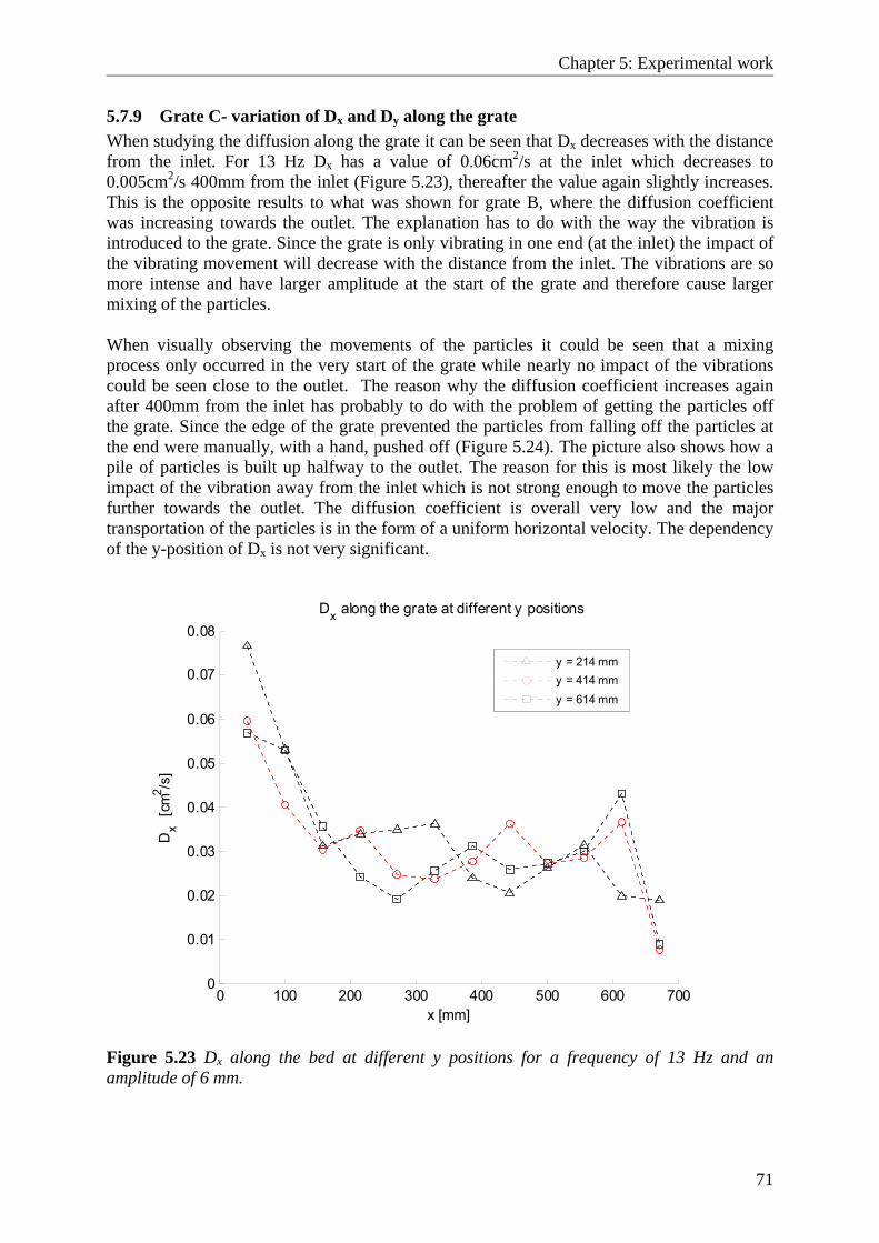
Chapter 5: Experimental work
71
5.7.9 Grate C- variation of Dx and Dy along the grate When studying the diffusion along the grate it can be seen that Dx decreases with the distance from the inlet. For 13 Hz Dx has a value of 0.06cm2/s at the inlet which decreases to 0.005cm2/s 400mm from the inlet (Figure 5.23), thereafter the value again slightly increases. This is the opposite results to what was shown for grate B, where the diffusion coefficient was increasing towards the outlet. The explanation has to do with the way the vibration is introduced to the grate. Since the grate is only vibrating in one end (at the inlet) the impact of the vibrating movement will decrease with the distance from the inlet. The vibrations are so more intense and have larger amplitude at the start of the grate and therefore cause larger mixing of the particles. When visually observing the movements of the particles it could be seen that a mixing process only occurred in the very start of the grate while nearly no impact of the vibrations could be seen close to the outlet. The reason why the diffusion coefficient increases again after 400mm from the inlet has probably to do with the problem of getting the particles off the grate. Since the edge of the grate prevented the particles from falling off the particles at the end were manually, with a hand, pushed off (Figure 5.24). The picture also shows how a pile of particles is built up halfway to the outlet. The reason for this is most likely the low impact of the vibration away from the inlet which is not strong enough to move the particles further towards the outlet. The diffusion coefficient is overall very low and the major transportation of the particles is in the form of a uniform horizontal velocity. The dependency of the y-position of Dx is not very significant.
0 100 200 300 400 500 600 7000
0.01
0.02
0.03
0.04
0.05
0.06
0.07
0.08Dx along the grate at different y positions
x [mm]
Dx [
cm2 /s
]
y = 214 mmy = 414 mmy = 614 mm
Figure 5.23 Dx along the bed at different y positions for a frequency of 13 Hz and an amplitude of 6 mm.
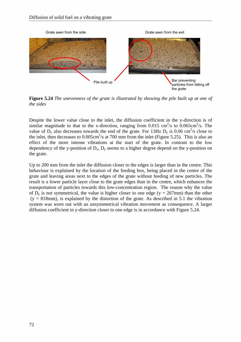
Diffusion of solid fuel on a vibrating grate
72
Figure 5.24 The unevenness of the grate is illustrated by showing the pile built up at one of the sides
Despite the lower value close to the inlet, the diffusion coefficient in the y-direction is of similar magnitude to that in the x-direction, ranging from 0.015 cm2/s to 0.065cm2/s. The value of Dy also decreases towards the end of the grate. For 13Hz Dy is 0.06 cm2/s close to the inlet, then decreases to 0.005cm2/s at 700 mm from the inlet (Figure 5.25). This is also an effect of the more intense vibrations at the start of the grate. In contrast to the low dependency of the y-position of Dx, Dy seems to a higher degree depend on the y-position on the grate. Up to 200 mm from the inlet the diffusion closer to the edges is larger than in the centre. This behaviour is explained by the location of the feeding box, being placed in the centre of the grate and leaving areas next to the edges of the grate without feeding of new particles. The result is a lower particle layer close to the grate edges than in the centre, which enhances the transportation of particles towards this low-concentration region. The reason why the value of Dy is not symmetrical, the value is higher closer to one edge (y = 267mm) than the other (y = 818mm), is explained by the distortion of the grate. As described in 5.1 the vibration system was worn out with an unsymmetrical vibration movement as consequence. A larger diffusion coefficient in y-direction closer to one edge is in accordance with Figure 5.24.
Grate seen from the side Grate seen from the exit
Pile built up Bar preventing particles from falling off the grate
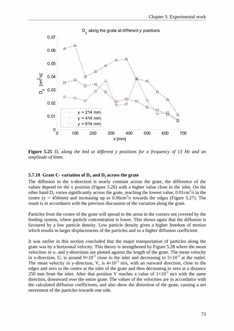
Chapter 5: Experimental work
73
0 100 200 300 400 500 600 7000
0.01
0.02
0.03
0.04
0.05
0.06
0.07Dy along the grate at different y positions
x [mm]
Dy [
cm2 /s
]
y = 214 mmy = 414 mmy = 614 mm
Figure 5.25 Dy along the bed at different y positions for a frequency of 13 Hz and an amplitude of 6mm.
5.7.10 Grate C- variation of Dx and Dy across the grate The diffusion in the x-direction is nearly constant across the grate, the difference of the values depend on the x position (Figure 5.26) with a higher value close to the inlet. On the other hand Dy varies significantly across the grate, reaching the lowest value, 0.01cm2/s in the centre (y = 450mm) and increasing up to 0.06cm2/s towards the edges (Figure 5.27). The result is in accordance with the previous discussion of the variation along the grate. Particles from the centre of the grate will spread to the areas in the corners not covered by the feeding system, where particle concentration is lower. This shows again that the diffusion is favoured by a low particle density. Low particle density gives a higher freedom of motion which results in larger displacements of the particles and so a higher diffusion coefficient. It was earlier in this section concluded that the major transportation of particles along the grate was by a horizontal velocity. This theory is strengthened by Figure 5.28 where the mean velocities in x- and y-directions are plotted against the length of the grate. The mean velocity in x-direction, U, is around 9×10⁻³ close to the inlet and decreasing to 5×10⁻³ at the outlet. The mean velocity in y-direction, V, is 4×10⁻³ m/s, with an outward direction, close to the edges and zero in the centre at the inlet of the grate and then decreasing to zero at a distance 250 mm from the inlet. After that position V reaches a value of 1×10⁻³ m/s with the same direction, downward over the entire grate. The values of the velocities are in accordance with the calculated diffusion coefficients, and also show the distortion of the grate, causing a net movement of the particles towards one side.
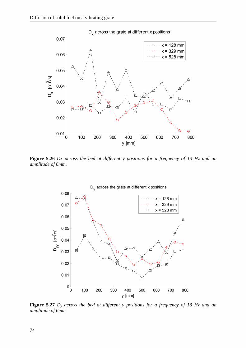
Diffusion of solid fuel on a vibrating grate
74
0 100 200 300 400 500 600 700 8000.01
0.02
0.03
0.04
0.05
0.06
0.07Dx across the grate at different x positions
y [mm]
Dx [
cm2 /s
]
x = 128 mmx = 329 mmx = 528 mm
Figure 5.26 Dx across the bed at different y positions for a frequency of 13 Hz and an amplitude of 6mm.
0 100 200 300 400 500 600 700 8000
0.01
0.02
0.03
0.04
0.05
0.06
0.07
0.08Dy across the grate at different x positions
y [mm]
Dyy
[cm
2 /s]
x = 128 mmx = 329 mmx = 528 mm
Figure 5.27 Dy across the bed at different y positions for a frequency of 13 Hz and an amplitude of 6mm.
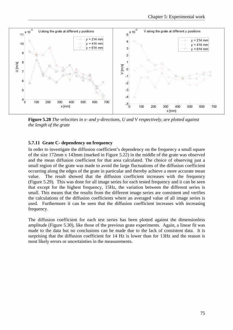
Chapter 5: Experimental work
75
0 100 200 300 400 500 600 7004
5
6
7
8
9
10
11x 10
-3 U along the grate at different y positions
x [mm]
U [m
/s]
y = 214 mmy = 414 mmy = 614 mm
0 100 200 300 400 500 600 700-5
-4
-3
-2
-1
0
1
2
3
4
5x 10
-3 V along the grate at different y positions
x [mm]
V [m
/s]
y = 214 mmy = 414 mmy = 614 mm
Figure 5.28 The velocities in x- and y-directions, U and V respectively, are plotted against the length of the grate
5.7.11 Grate C- dependency on frequency In order to investigate the diffusion coefficient’s dependency on the frequency a small square of the size 172mm x 143mm (marked in Figure 5.22) in the middle of the grate was observed and the mean diffusion coefficient for that area calculated. The choice of observing just a small region of the grate was made to avoid the large fluctuations of the diffusion coefficient occurring along the edges of the grate in particular and thereby achieve a more accurate mean value. The result showed that the diffusion coefficient increases with the frequency (Figure 5.29). This was done for all image series for each tested frequency and it can be seen that except for the highest frequency, 15Hz, the variation between the different series is small. This means that the results from the different image series are consistent and verifies the calculations of the diffusion coefficients where an averaged value of all image series is used. Furthermore it can be seen that the diffusion coefficient increases with increasing frequency. The diffusion coefficient for each test series has been plotted against the dimensionless amplitude (Figure 5.30), like those of the previous grate experiments. Again, a linear fit was made to the data but no conclusions can be made due to the lack of consistent data. It is surprising that the diffusion coefficient for 14 Hz is lower than for 13Hz and the reason is most likely errors or uncertainties in the measurements.
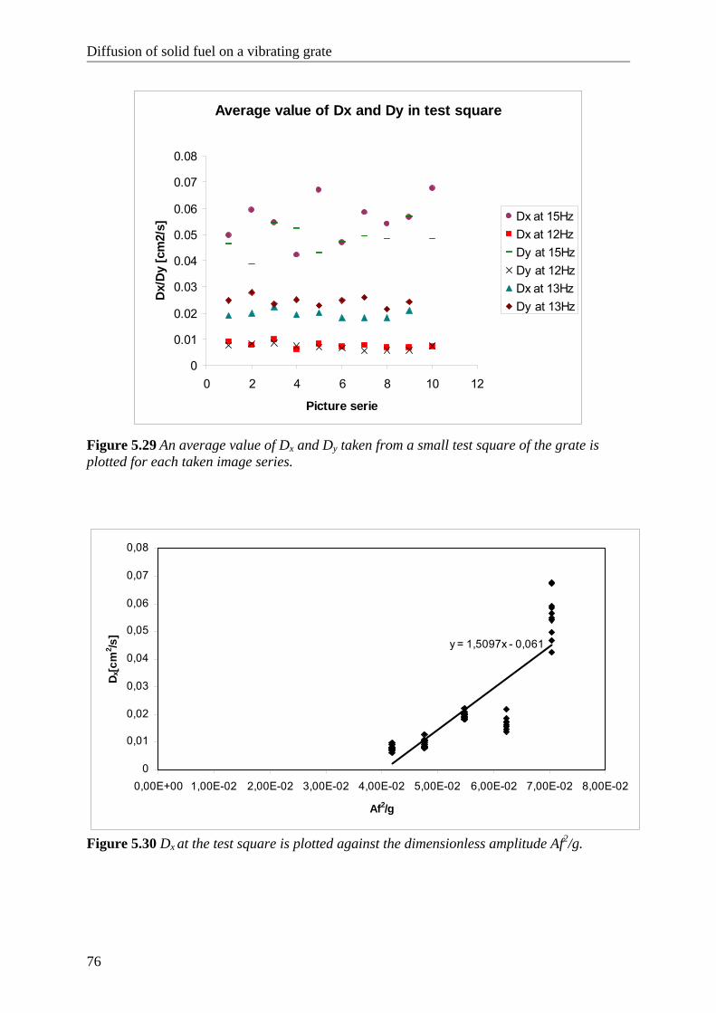
Diffusion of solid fuel on a vibrating grate
76
Average value of Dx and Dy in test square
0
0.01
0.02
0.03
0.04
0.05
0.06
0.07
0.08
0 2 4 6 8 10 12
Picture serie
Dx/
Dy
[cm
2/s]
Dx at 15HzDx at 12HzDy at 15HzDy at 12HzDx at 13HzDy at 13Hz
Figure 5.29 An average value of Dx and Dy taken from a small test square of the grate is plotted for each taken image series.
y = 1,5097x - 0,061
0
0,01
0,02
0,03
0,04
0,05
0,06
0,07
0,08
0,00E+00 1,00E-02 2,00E-02 3,00E-02 4,00E-02 5,00E-02 6,00E-02 7,00E-02 8,00E-02
Af2/g
D x[c
m2 /s
]
Figure 5.30 Dx at the test square is plotted against the dimensionless amplitude Af2/g.
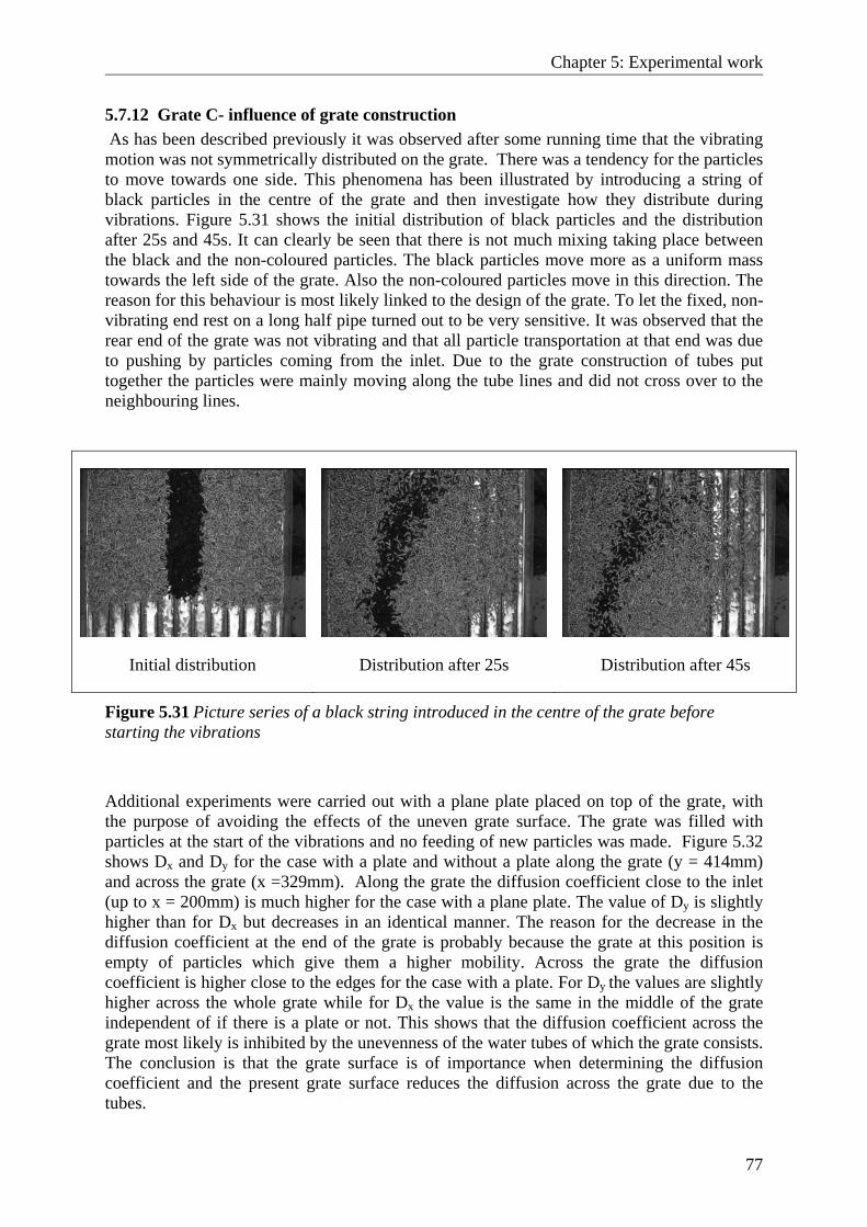
Chapter 5: Experimental work
77
5.7.12 Grate C- influence of grate construction As has been described previously it was observed after some running time that the vibrating motion was not symmetrically distributed on the grate. There was a tendency for the particles to move towards one side. This phenomena has been illustrated by introducing a string of black particles in the centre of the grate and then investigate how they distribute during vibrations. Figure 5.31 shows the initial distribution of black particles and the distribution after 25s and 45s. It can clearly be seen that there is not much mixing taking place between the black and the non-coloured particles. The black particles move more as a uniform mass towards the left side of the grate. Also the non-coloured particles move in this direction. The reason for this behaviour is most likely linked to the design of the grate. To let the fixed, non- vibrating end rest on a long half pipe turned out to be very sensitive. It was observed that the rear end of the grate was not vibrating and that all particle transportation at that end was due to pushing by particles coming from the inlet. Due to the grate construction of tubes put together the particles were mainly moving along the tube lines and did not cross over to the neighbouring lines.
Initial distribution
Distribution after 25s Distribution after 45s
Figure 5.31 Picture series of a black string introduced in the centre of the grate before starting the vibrations
Additional experiments were carried out with a plane plate placed on top of the grate, with the purpose of avoiding the effects of the uneven grate surface. The grate was filled with particles at the start of the vibrations and no feeding of new particles was made. Figure 5.32 shows Dx and Dy for the case with a plate and without a plate along the grate (y = 414mm) and across the grate (x =329mm). Along the grate the diffusion coefficient close to the inlet (up to x = 200mm) is much higher for the case with a plane plate. The value of Dy is slightly higher than for Dx but decreases in an identical manner. The reason for the decrease in the diffusion coefficient at the end of the grate is probably because the grate at this position is empty of particles which give them a higher mobility. Across the grate the diffusion coefficient is higher close to the edges for the case with a plate. For Dy the values are slightly higher across the whole grate while for Dx the value is the same in the middle of the grate independent of if there is a plate or not. This shows that the diffusion coefficient across the grate most likely is inhibited by the unevenness of the water tubes of which the grate consists. The conclusion is that the grate surface is of importance when determining the diffusion coefficient and the present grate surface reduces the diffusion across the grate due to the tubes.
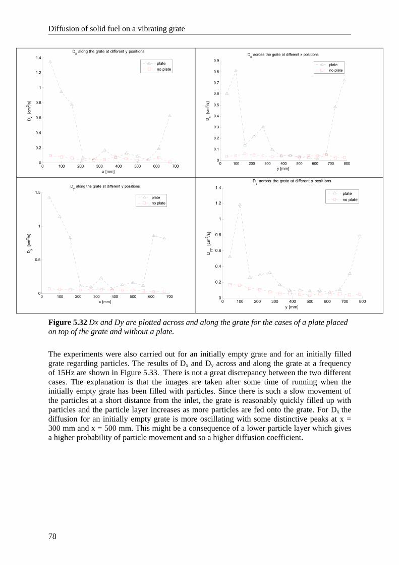
Diffusion of solid fuel on a vibrating grate
78
0 100 200 300 400 500 600 7000
0.2
0.4
0.6
0.8
1
1.2
1.4Dx along the grate at different y positions
x [mm]
Dx [
cm2 /s
]
plateno plate
0 100 200 300 400 500 600 700 8000
0.1
0.2
0.3
0.4
0.5
0.6
0.7
0.8
0.9Dx across the grate at different x positions
y [mm]
Dx [
cm2 /s
]
plateno plate
0 100 200 300 400 500 600 7000
0.5
1
1.5Dy along the grate at different y positions
x [mm]
Dy [
cm2 /s
]
plateno plate
0 100 200 300 400 500 600 700 8000
0.2
0.4
0.6
0.8
1
1.2
1.4Dy across the grate at different x positions
y [mm]
Dyy
[cm
2 /s]
plateno plate
Figure 5.32 Dx and Dy are plotted across and along the grate for the cases of a plate placed on top of the grate and without a plate.
The experiments were also carried out for an initially empty grate and for an initially filled grate regarding particles. The results of Dx and Dy across and along the grate at a frequency of 15Hz are shown in Figure 5.33. There is not a great discrepancy between the two different cases. The explanation is that the images are taken after some time of running when the initially empty grate has been filled with particles. Since there is such a slow movement of the particles at a short distance from the inlet, the grate is reasonably quickly filled up with particles and the particle layer increases as more particles are fed onto the grate. For Dx the diffusion for an initially empty grate is more oscillating with some distinctive peaks at x = 300 mm and x = 500 mm. This might be a consequence of a lower particle layer which gives a higher probability of particle movement and so a higher diffusion coefficient.
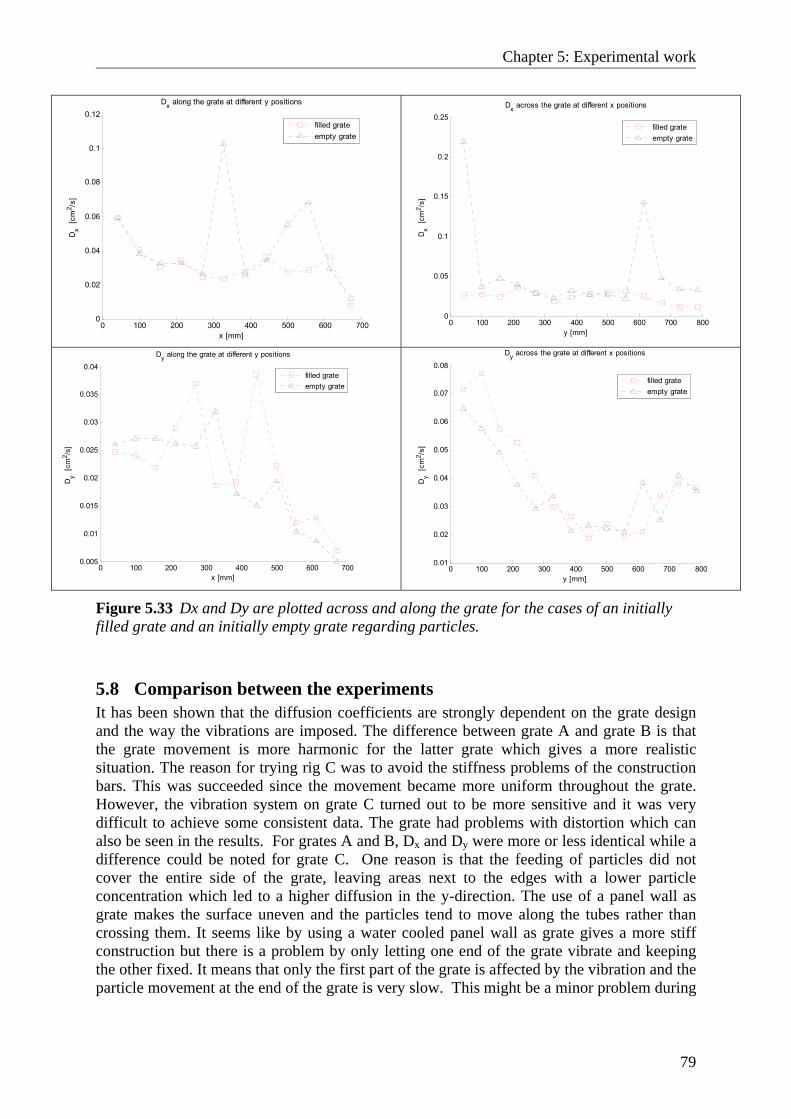
Chapter 5: Experimental work
79
0 100 200 300 400 500 600 7000
0.02
0.04
0.06
0.08
0.1
0.12Dx along the grate at different y positions
x [mm]
Dx [
cm2 /s
]
filled grateempty grate
0 100 200 300 400 500 600 700 8000
0.05
0.1
0.15
0.2
0.25Dx across the grate at different x positions
y [mm]
Dx [
cm2 /s
]
filled grateempty grate
0 100 200 300 400 500 600 7000.005
0.01
0.015
0.02
0.025
0.03
0.035
0.04
Dy along the grate at different y positions
x [mm]
Dy [
cm2 /s
]
filled grateempty grate
0 100 200 300 400 500 600 700 800
0.01
0.02
0.03
0.04
0.05
0.06
0.07
0.08
Dy across the grate at different x positions
y [mm]
Dy [
cm2 /s
]
filled grateempty grate
Figure 5.33 Dx and Dy are plotted across and along the grate for the cases of an initially filled grate and an initially empty grate regarding particles.
5.8 Comparison between the experiments It has been shown that the diffusion coefficients are strongly dependent on the grate design and the way the vibrations are imposed. The difference between grate A and grate B is that the grate movement is more harmonic for the latter grate which gives a more realistic situation. The reason for trying rig C was to avoid the stiffness problems of the construction bars. This was succeeded since the movement became more uniform throughout the grate. However, the vibration system on grate C turned out to be more sensitive and it was very difficult to achieve some consistent data. The grate had problems with distortion which can also be seen in the results. For grates A and B, Dx and Dy were more or less identical while a difference could be noted for grate C. One reason is that the feeding of particles did not cover the entire side of the grate, leaving areas next to the edges with a lower particle concentration which led to a higher diffusion in the y-direction. The use of a panel wall as grate makes the surface uneven and the particles tend to move along the tubes rather than crossing them. It seems like by using a water cooled panel wall as grate gives a more stiff construction but there is a problem by only letting one end of the grate vibrate and keeping the other fixed. It means that only the first part of the grate is affected by the vibration and the particle movement at the end of the grate is very slow. This might be a minor problem during
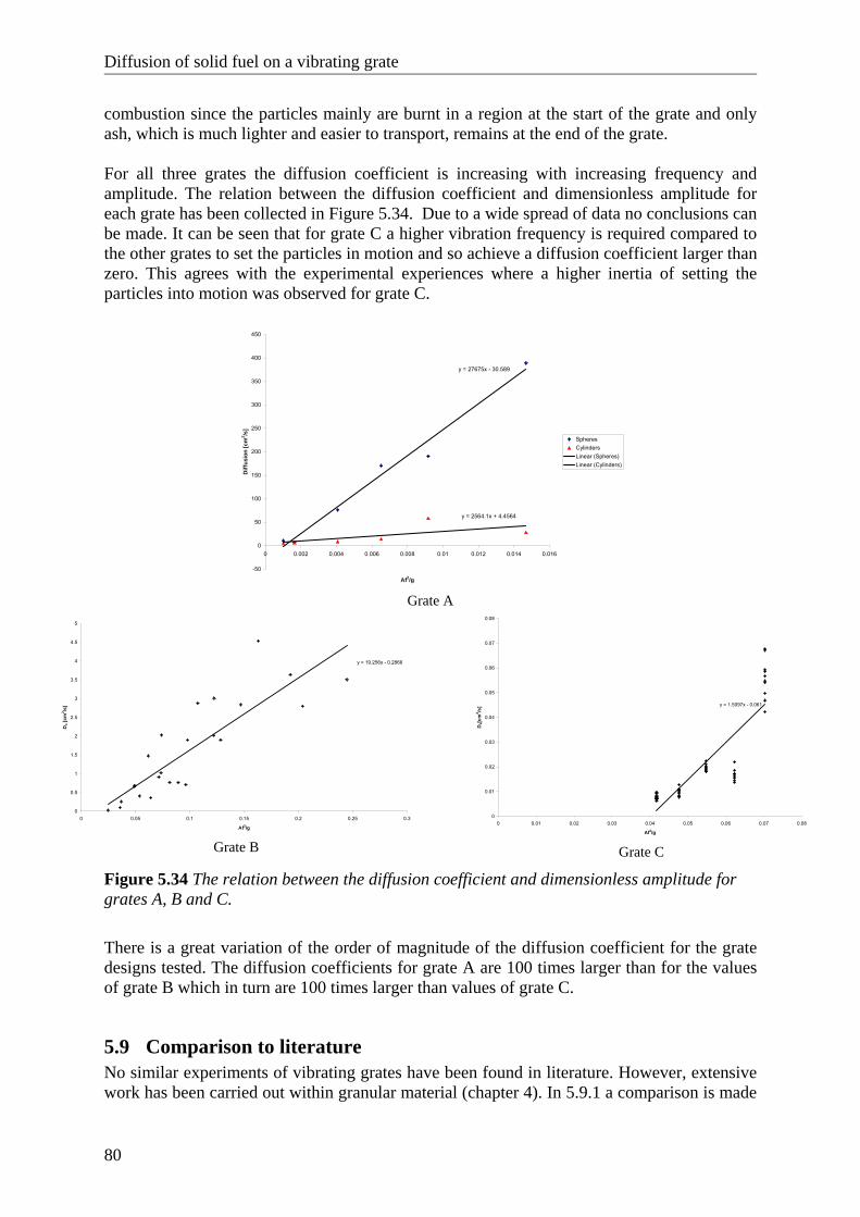
Diffusion of solid fuel on a vibrating grate
80
combustion since the particles mainly are burnt in a region at the start of the grate and only ash, which is much lighter and easier to transport, remains at the end of the grate. For all three grates the diffusion coefficient is increasing with increasing frequency and amplitude. The relation between the diffusion coefficient and dimensionless amplitude for each grate has been collected in Figure 5.34. Due to a wide spread of data no conclusions can be made. It can be seen that for grate C a higher vibration frequency is required compared to the other grates to set the particles in motion and so achieve a diffusion coefficient larger than zero. This agrees with the experimental experiences where a higher inertia of setting the particles into motion was observed for grate C.
y = 27675x - 30.589
y = 2564.1x + 4.4564
-50
0
50
100
150
200
250
300
350
400
450
0 0.002 0.004 0.006 0.008 0.01 0.012 0.014 0.016
Af2/g
Diff
usio
n [c
m2 /s
]
SpheresCylindersLinear (Spheres)Linear (Cylinders)
Grate A
y = 19.256x - 0.2866
0
0.5
1
1.5
2
2.5
3
3.5
4
4.5
5
0 0.05 0.1 0.15 0.2 0.25 0.3
Af2/g
Dx [
cm2 /s
]
Grate B
y = 1.5097x - 0.061
0
0.01
0.02
0.03
0.04
0.05
0.06
0.07
0.08
0 0.01 0.02 0.03 0.04 0.05 0.06 0.07 0.08
Af2/g
Dx[c
m2 /s
]
Grate C
Figure 5.34 The relation between the diffusion coefficient and dimensionless amplitude for grates A, B and C. There is a great variation of the order of magnitude of the diffusion coefficient for the grate designs tested. The diffusion coefficients for grate A are 100 times larger than for the values of grate B which in turn are 100 times larger than values of grate C.
5.9 Comparison to literature No similar experiments of vibrating grates have been found in literature. However, extensive work has been carried out within granular material (chapter 4). In 5.9.1 a comparison is made
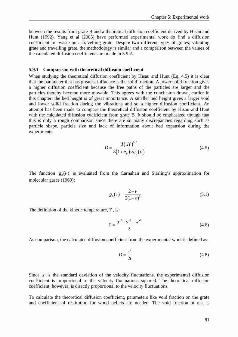
Chapter 5: Experimental work
81
between the results from grate B and a theoretical diffusion coefficient derived by Hisau and Hunt (1992). Yang et al (2005) have performed experimental work do find a diffusion coefficient for waste on a travelling grate. Despite two different types of grates; vibrating grate and travelling grate, the methodology is similar and a comparison between the values of the calculated diffusion coefficients are made in 5.9.2.
5.9.1 Comparison with theoretical diffusion coefficient When studying the theoretical diffusion coefficient by Hisau and Hunt (Eq. 4.5) it is clear that the parameter that has greatest influence is the solid fraction. A lower solid fraction gives a higher diffusion coefficient because the free paths of the particles are larger and the particles thereby become more movable. This agrees with the conclusion drawn, earlier in this chapter: the bed height is of great importance. A smaller bed height gives a larger void and lower solid fraction during the vibrations and so a higher diffusion coefficient. An attempt has been made to compare the theoretical diffusion coefficient by Hisau and Hunt with the calculated diffusion coefficient from grate B. It should be emphasized though that this is only a rough comparison since there are so many discrepancies regarding such as particle shape, particle size and lack of information about bed expansion during the experiments.
( )( ) ( )
1/ 2
08 1 p
dD
e gπν νϒ
=+
(4.5)
The function 0 ( )g ν is evaluated from the Carnahan and Starling’s approximation for molecular gases (1969):
0 3
2( )2(1 )
g ννν−
=−
(5.1)
The definition of the kinetic temperature,ϒ , is:
2 2 2' ' '
3u v w+ +
ϒ = (4.6)
As comparison, the calculated diffusion coefficient from the experimental work is defined as:
2
2sDt
= (4.8)
Since s is the standard deviation of the velocity fluctuations, the experimental diffusion coefficient is proportional to the velocity fluctuations squared. The theoretical diffusion coefficient, however, is directly proportional to the velocity fluctuations. To calculate the theoretical diffusion coefficient, parameters like void fraction on the grate and coefficient of restitution for wood pellets are needed. The void fraction at rest is
Diffusion of solid fuel on a vibrating grate
82
estimated to 0.5 and since the expansion is fairly low the same value has been used for the calculations. The coefficient of restitution is set to 0.95. This is only an estimation not based on any specific measurements but the choice of the coefficient of restitution is not of great importance for the results which can be seen in Eq. (4.5), the void fraction is more important due to the third power influence. When calculating the granular temperature the velocity fluctuations are used. These values are taken from the standard deviation of the velocity from the taken image series during the experimental work. The two different calculations are based on the same parameters and the results show that the velocity fluctuations are the determining values for the diffusion coefficient. When calculating the theoretical diffusions coefficient different values of the solid fraction are tested. It can be seen that for lower frequencies and amplitudes a higher value of the solid fraction fits better to the experimental diffusion coefficient. For a higher frequency and amplitude the movement of the particles is greater with a larger bed expansion which gives a lower solid fraction. It can also be seen that the theoretical diffusion coefficient close to the outlet fits better to the calculated value at a lower solid fraction. This agrees well with the observations made during the experimental work; the particle depth decreases towards the outlet which means a higher particle motion and so a lower solid fraction. As a result of the comparison it could be concluded that the theoretical diffusion coefficient can be used in order to calculate the void fraction. The relation between the diffusion coefficient and porosity of the bed is interesting since the porosity is the connection point between the gas phase and solid phase. This would be very useful when simulating the gas phase and a further investigation is recommended.
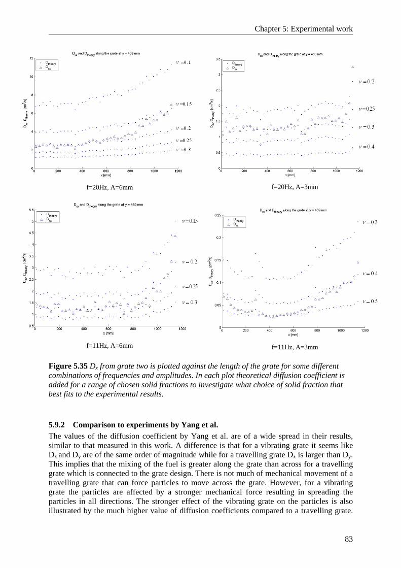
Chapter 5: Experimental work
83
f=20Hz, A=6mm
f=20Hz, A=3mm
f=11Hz, A=6mm
f=11Hz, A=3mm
Figure 5.35 Dx from grate two is plotted against the length of the grate for some different combinations of frequencies and amplitudes. In each plot theoretical diffusion coefficient is added for a range of chosen solid fractions to investigate what choice of solid fraction that best fits to the experimental results.
5.9.2 Comparison to experiments by Yang et al. The values of the diffusion coefficient by Yang et al. are of a wide spread in their results, similar to that measured in this work. A difference is that for a vibrating grate it seems like Dx and Dy are of the same order of magnitude while for a travelling grate Dx is larger than Dy. This implies that the mixing of the fuel is greater along the grate than across for a travelling grate which is connected to the grate design. There is not much of mechanical movement of a travelling grate that can force particles to move across the grate. However, for a vibrating grate the particles are affected by a stronger mechanical force resulting in spreading the particles in all directions. The stronger effect of the vibrating grate on the particles is also illustrated by the much higher value of diffusion coefficients compared to a travelling grate.
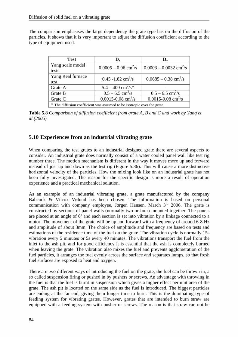
Diffusion of solid fuel on a vibrating grate
84
The comparison emphasises the large dependency the grate type has on the diffusion of the particles. It shows that it is very important to adjust the diffusion coefficient according to the type of equipment used.
Test Dx Dy Yang scale model tests 0.0005 – 0.06 cm2/s 0.0003 – 0.0032 cm2/s
Yang Real furnace test 0.45 -1.82 cm2/s 0.0685 – 0.38 cm2/s
Grate A 5.4 – 400 cm2/s* - Grate B 0.5 – 6.5 cm2/s 0.5 – 6.5 cm2/s Grate C 0.0015-0.08 cm2/s 0.0015-0.08 cm2/s * The diffusion coefficient was assumed to be isotropic over the grate
Table 5.8 Comparison of diffusion coefficient from grate A, B and C and work by Yang et. al.(2005).
5.10 Experiences from an industrial vibrating grate When comparing the test grates to an industrial designed grate there are several aspects to consider. An industrial grate does normally consist of a water cooled panel wall like test rig number three. The motion mechanism is different in the way it moves more up and forward instead of just up and down as the test rig (Figure 5.36). This will cause a more distinctive horizontal velocity of the particles. How the mixing look like on an industrial grate has not been fully investigated. The reason for the specific design is more a result of operation experience and a practical mechanical solution. As an example of an industrial vibrating grate, a grate manufactured by the company Babcock & Vilcox Vølund has been chosen. The information is based on personal communication with company employee, Jørgen Hansen, March 3rd 2006. The grate is constructed by sections of panel walls (normally two or four) mounted together. The panels are placed at an angle of 6º and each section is set into vibration by a linkage connected to a motor. The movement of the grate will be up and forward with a frequency of around 6-8 Hz and amplitude of about 3mm. The choice of amplitude and frequency are based on tests and estimations of the residence time of the fuel on the grate. The vibration cycle is normally 15s vibration every 5 minutes or 5s every 40 minutes. The vibrations transport the fuel from the inlet to the ash pit, and for good efficiency it is essential that the ash is completely burned when leaving the grate. The vibration also mixes the fuel and prevents agglomeration of the fuel particles, it arranges the fuel evenly across the surface and separates lumps, so that fresh fuel surfaces are exposed to heat and oxygen. There are two different ways of introducing the fuel on the grate; the fuel can be thrown in, a so called suspension firing or pushed in by pushers or screws. An advantage with throwing in the fuel is that the fuel is burnt in suspension which gives a higher effect per unit area of the grate. The ash pit is located on the same side as the fuel is introduced. The biggest particles are ending at the far end, giving them longer time to burn. This is the dominating type of feeding system for vibrating grates. However, grates that are intended to burn straw are equipped with a feeding system with pusher or screws. The reason is that straw can not be
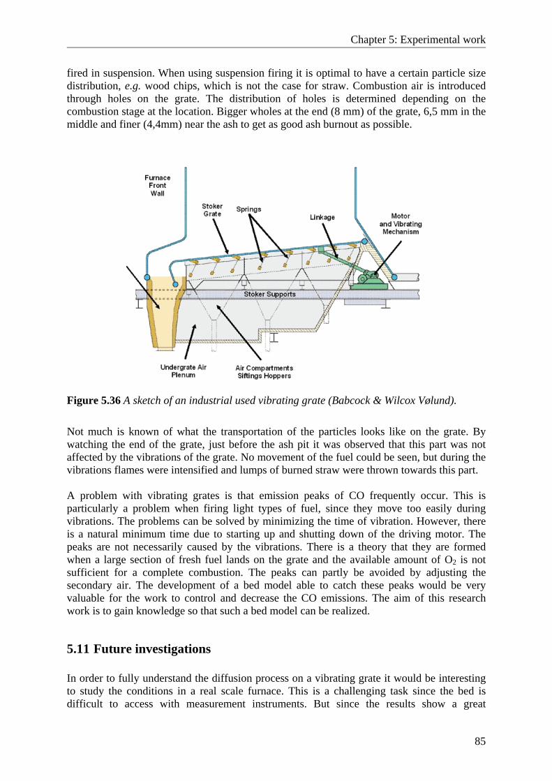
Chapter 5: Experimental work
85
fired in suspension. When using suspension firing it is optimal to have a certain particle size distribution, e.g. wood chips, which is not the case for straw. Combustion air is introduced through holes on the grate. The distribution of holes is determined depending on the combustion stage at the location. Bigger wholes at the end (8 mm) of the grate, 6,5 mm in the middle and finer (4,4mm) near the ash to get as good ash burnout as possible.
Figure 5.36 A sketch of an industrial used vibrating grate (Babcock & Wilcox Vølund).
Not much is known of what the transportation of the particles looks like on the grate. By watching the end of the grate, just before the ash pit it was observed that this part was not affected by the vibrations of the grate. No movement of the fuel could be seen, but during the vibrations flames were intensified and lumps of burned straw were thrown towards this part. A problem with vibrating grates is that emission peaks of CO frequently occur. This is particularly a problem when firing light types of fuel, since they move too easily during vibrations. The problems can be solved by minimizing the time of vibration. However, there is a natural minimum time due to starting up and shutting down of the driving motor. The peaks are not necessarily caused by the vibrations. There is a theory that they are formed when a large section of fresh fuel lands on the grate and the available amount of O2 is not sufficient for a complete combustion. The peaks can partly be avoided by adjusting the secondary air. The development of a bed model able to catch these peaks would be very valuable for the work to control and decrease the CO emissions. The aim of this research work is to gain knowledge so that such a bed model can be realized.
5.11 Future investigations In order to fully understand the diffusion process on a vibrating grate it would be interesting to study the conditions in a real scale furnace. This is a challenging task since the bed is difficult to access with measurement instruments. But since the results show a great
Diffusion of solid fuel on a vibrating grate
86
dependency of the chosen vibrating system, real scale experiments are vital. It is also necessary to look further into the vertical vibration process. According to theory of granular material the diffusion is highest in the direction of vibration which in this case is the vertical direction. It has been found that the bed height is of great importance when determining the diffusion coefficient and further studies need to be undertaken regarding how, more exactly, the diffusion coefficient depend on the bed height.
5.12 Conclusion / Summary
The large difference of diffusion coefficient in the different experiments means that a theoretical diffusion coefficient will be difficult to derive. Instead the best way would be to determine the diffusion coefficient experimentally or empirically. It is clear that the diffusion coefficient should vary with the location in the bed and with the intensity of the vibrations. The nature of this variation will most likely look the same independently of the grate system, and has been examined and presented in this chapter. The major findings from the experimental work are:
• Dx and Dy are of the same magnitude.
• Grate construction and vibrating system is of great importance for the diffusion coefficient.
• Dx and Dy increases with increasing frequency and amplitude.
• Dx and Dy increases with decreasing particle thickness. There is also a possibility that the combustion process will have an effect on the diffusion coefficient. However, by studying the behaviour of particle transportation with no combustion taken place, the overall mechanisms can be identified and quantified. Knowing these mechanisms will be of significant help when, in the future, investigating the mixing process of fuel in a burning bed.
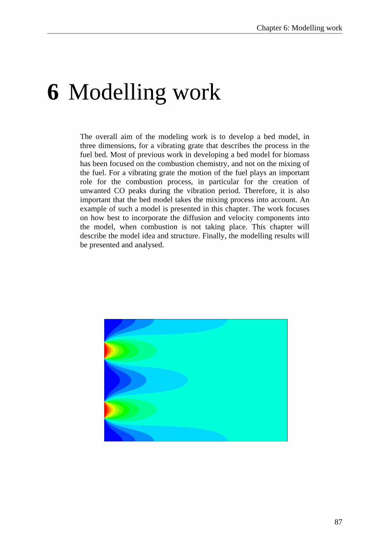
Chapter 6: Modelling work
87
6 Modelling work
The overall aim of the modeling work is to develop a bed model, in three dimensions, for a vibrating grate that describes the process in the fuel bed. Most of previous work in developing a bed model for biomass has been focused on the combustion chemistry, and not on the mixing of the fuel. For a vibrating grate the motion of the fuel plays an important role for the combustion process, in particular for the creation of unwanted CO peaks during the vibration period. Therefore, it is also important that the bed model takes the mixing process into account. An example of such a model is presented in this chapter. The work focuses on how best to incorporate the diffusion and velocity components into the model, when combustion is not taking place. This chapter will describe the model idea and structure. Finally, the modelling results will be presented and analysed.
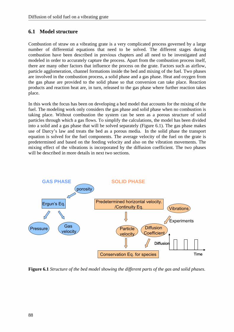
Diffusion of solid fuel on a vibrating grate
88
6.1 Model structure Combustion of straw on a vibrating grate is a very complicated process governed by a large number of differential equations that need to be solved. The different stages during combustion have been described in previous chapters and all need to be investigated and modeled in order to accurately capture the process. Apart from the combustion process itself, there are many other factors that influence the process on the grate. Factors such as airflow, particle agglomeration, channel formations inside the bed and mixing of the fuel. Two phases are involved in the combustion process, a solid phase and a gas phase. Heat and oxygen from the gas phase are provided to the solid phase so that conversion can take place. Reaction products and reaction heat are, in turn, released to the gas phase where further reaction takes place. In this work the focus has been on developing a bed model that accounts for the mixing of the fuel. The modeling work only considers the gas phase and solid phase when no combustion is taking place. Without combustion the system can be seen as a porous structure of solid particles through which a gas flows. To simplify the calculations, the model has been divided into a solid and a gas phase that will be solved separately (Figure 6.1). The gas phase makes use of Darcy’s law and treats the bed as a porous media. In the solid phase the transport equation is solved for the fuel components. The average velocity of the fuel on the grate is predetermined and based on the feeding velocity and also on the vibration movements. The mixing effect of the vibrations is incorporated by the diffusion coefficient. The two phases will be described in more details in next two sections.
Predetermined horizontal velocity./Continuity Eq.
Ergun’s Eq.
porosity
Gas velocityPressure Particle
velocity
Vibrations
Diffusion Coefficient
GAS PHASE SOLID PHASE
Experiments
Diffusion
Time
Diffusion
TimeConservation Eq. for species
Figure 6.1 Structure of the bed model showing the different parts of the gas and solid phases.
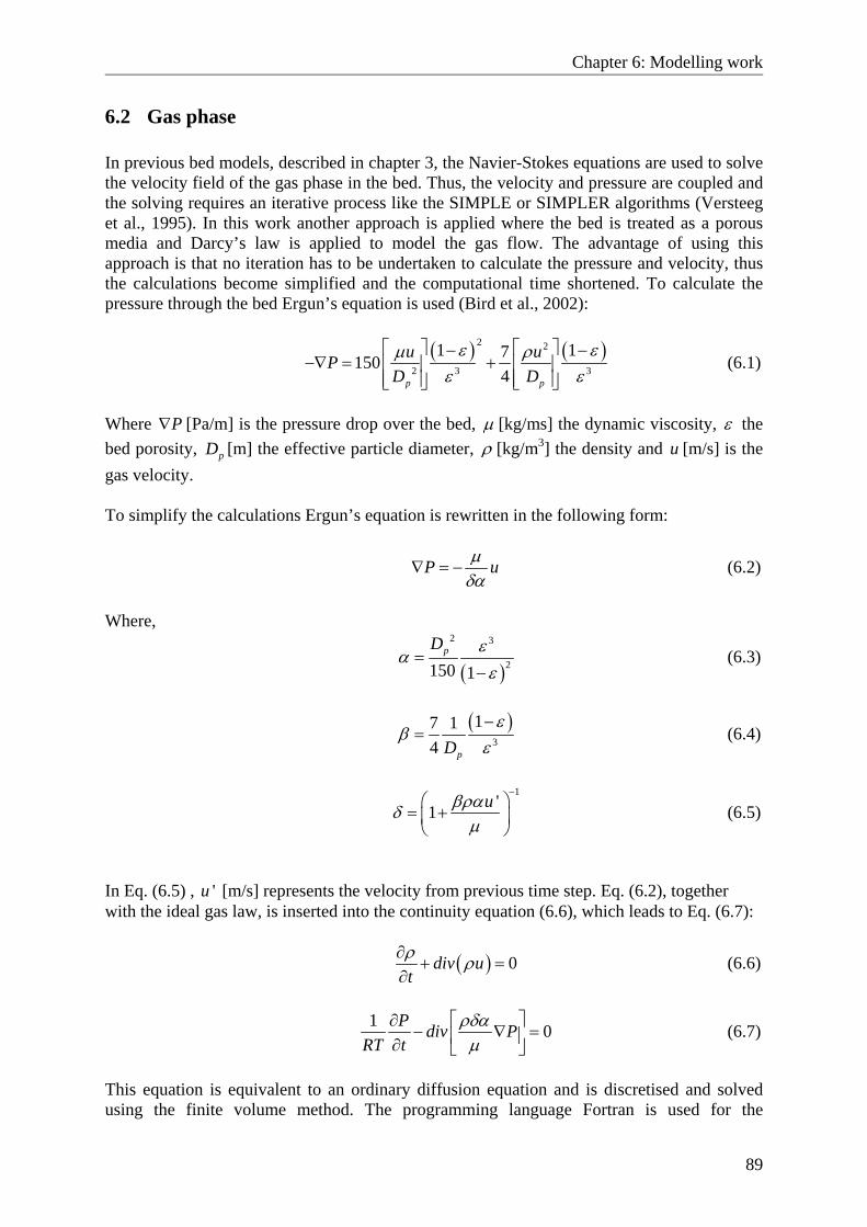
Chapter 6: Modelling work
89
6.2 Gas phase In previous bed models, described in chapter 3, the Navier-Stokes equations are used to solve the velocity field of the gas phase in the bed. Thus, the velocity and pressure are coupled and the solving requires an iterative process like the SIMPLE or SIMPLER algorithms (Versteeg et al., 1995). In this work another approach is applied where the bed is treated as a porous media and Darcy’s law is applied to model the gas flow. The advantage of using this approach is that no iteration has to be undertaken to calculate the pressure and velocity, thus the calculations become simplified and the computational time shortened. To calculate the pressure through the bed Ergun’s equation is used (Bird et al., 2002):
( ) ( )2 2
2 3 3
1 171504p p
u uPD D
ε εμ ρε ε
⎡ ⎤ ⎡ ⎤− −−∇ = +⎢ ⎥ ⎢ ⎥
⎢ ⎥ ⎢ ⎥⎣ ⎦ ⎣ ⎦ (6.1)
Where P∇ [Pa/m] is the pressure drop over the bed, μ [kg/ms] the dynamic viscosity, ε the bed porosity, pD [m] the effective particle diameter, ρ [kg/m3] the density and u [m/s] is the gas velocity. To simplify the calculations Ergun’s equation is rewritten in the following form:
P uμδα
∇ = − (6.2)
Where,
( )
2 3
2150 1pD εα
ε=
− (6.3)
( )3
17 14 pD
εβ
ε−
= (6.4)
1
'1 uβραδμ
−⎛ ⎞
= +⎜ ⎟⎝ ⎠
(6.5)
In Eq. (6.5) , 'u [m/s] represents the velocity from previous time step. Eq. (6.2), together with the ideal gas law, is inserted into the continuity equation (6.6), which leads to Eq. (6.7):
( ) 0div utρ ρ∂+ =
∂ (6.6)
1 0P div PRT t
ρδαμ
⎡ ⎤∂− ∇ =⎢ ⎥∂ ⎣ ⎦
(6.7)
This equation is equivalent to an ordinary diffusion equation and is discretised and solved using the finite volume method. The programming language Fortran is used for the
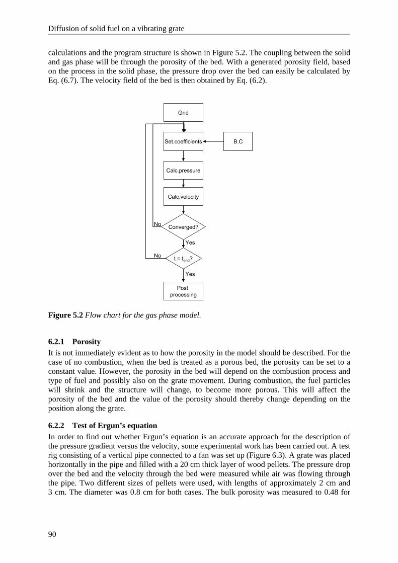
Diffusion of solid fuel on a vibrating grate
90
calculations and the program structure is shown in Figure 5.2. The coupling between the solid and gas phase will be through the porosity of the bed. With a generated porosity field, based on the process in the solid phase, the pressure drop over the bed can easily be calculated by Eq. (6.7). The velocity field of the bed is then obtained by Eq. (6.2).
Grid
Set.coefficients B.C
Calc.velocity
Post processing
Calc.pressure
Converged?
t = tend?
Yes
Yes
No
No
Figure 5.2 Flow chart for the gas phase model.
6.2.1 Porosity It is not immediately evident as to how the porosity in the model should be described. For the case of no combustion, when the bed is treated as a porous bed, the porosity can be set to a constant value. However, the porosity in the bed will depend on the combustion process and type of fuel and possibly also on the grate movement. During combustion, the fuel particles will shrink and the structure will change, to become more porous. This will affect the porosity of the bed and the value of the porosity should thereby change depending on the position along the grate.
6.2.2 Test of Ergun’s equation In order to find out whether Ergun’s equation is an accurate approach for the description of the pressure gradient versus the velocity, some experimental work has been carried out. A test rig consisting of a vertical pipe connected to a fan was set up (Figure 6.3). A grate was placed horizontally in the pipe and filled with a 20 cm thick layer of wood pellets. The pressure drop over the bed and the velocity through the bed were measured while air was flowing through the pipe. Two different sizes of pellets were used, with lengths of approximately 2 cm and 3 cm. The diameter was 0.8 cm for both cases. The bulk porosity was measured to 0.48 for
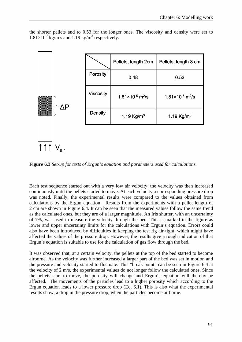
Chapter 6: Modelling work
91
the shorter pellets and to 0.53 for the longer ones. The viscosity and density were set to 1.81×10⁻⁵ kg/m s and 1.19 kg/m3 respectively.
ΔP
Vair
1.19 Kg/m31.19 Kg/m3Density
1.81×10⁻⁵ m2/s1.81×10-5 m2/sViscosity
0.530.48Porosity
Pellets, length 3 cmPellets, length 2cm
1.19 Kg/m31.19 Kg/m3Density
1.81×10⁻⁵ m2/s1.81×10-5 m2/sViscosity
0.530.48Porosity
Pellets, length 3 cmPellets, length 2cm
Figure 6.3 Set-up for tests of Ergun’s equation and parameters used for calculations.
Each test sequence started out with a very low air velocity, the velocity was then increased continuously until the pellets started to move. At each velocity a corresponding pressure drop was noted. Finally, the experimental results were compared to the values obtained from calculations by the Ergun equation. Results from the experiments with a pellet length of 2 cm are shown in Figure 6.4. It can be seen that the measured values follow the same trend as the calculated ones, but they are of a larger magnitude. An Iris shutter, with an uncertainty of 7%, was used to measure the velocity through the bed. This is marked in the figure as lower and upper uncertainty limits for the calculations with Ergun’s equation. Errors could also have been introduced by difficulties in keeping the test rig air-tight, which might have affected the values of the pressure drop. However, the results give a rough indication of that Ergun’s equation is suitable to use for the calculation of gas flow through the bed. It was observed that, at a certain velocity, the pellets at the top of the bed started to become airborne. As the velocity was further increased a larger part of the bed was set in motion and the pressure and velocity started to fluctuate. This “break point” can be seen in Figure 6.4 at the velocity of 2 m/s, the experimental values do not longer follow the calculated ones. Since the pellets start to move, the porosity will change and Ergun’s equation will thereby be affected. The movements of the particles lead to a higher porosity which according to the Ergun equation leads to a lower pressure drop (Eq. 6.1). This is also what the experimental results show, a drop in the pressure drop, when the particles become airborne.
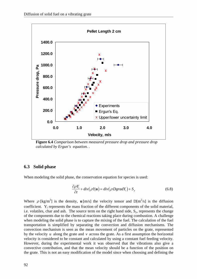
Diffusion of solid fuel on a vibrating grate
92
Pellet Length 2 cm
0.0
200.0
400.0
600.0
800.0
1000.0
1200.0
1400.0
0.0 1.0 2.0 3.0 4.0
Velocity, m/s
Pres
sure
dro
p, P
a
ExperimentsErgun's Eq. Upper/lower uncertainty limit
Figure 6.4 Comparison between measured pressure drop and pressure drop calculated by Ergun’s equation. .
6.3 Solid phase When modeling the solid phase, the conservation equation for species is used:
( ) ( )ii i y
Y div Y div DgradY Stρ ρ ρ∂
+ = +∂
u (6.8)
Where ρ [kg/m3] is the density, u [m/s] the velocity tensor and D[m2/s] is the diffusion coefficient. Yi represents the mass fraction of the different components of the solid material, i.e. volatiles, char and ash. The source term on the right hand side, Sy, represents the change of the components due to the chemical reactions taking place during combustion. A challenge when modeling the solid phase is to capture the mixing of the fuel. The calculation of the fuel transportation is simplified by separating the convection and diffusion mechanisms. The convection mechanism is seen as the mean movement of particles on the grate, represented by the velocity u along the grate and v across the grate. As a first assumption the horizontal velocity is considered to be constant and calculated by using a constant fuel feeding velocity. However, during the experimental work it was observed that the vibrations also give a convective contribution, and that the mean velocity should be a function of the position on the grate. This is not an easy modification of the model since when choosing and defining the
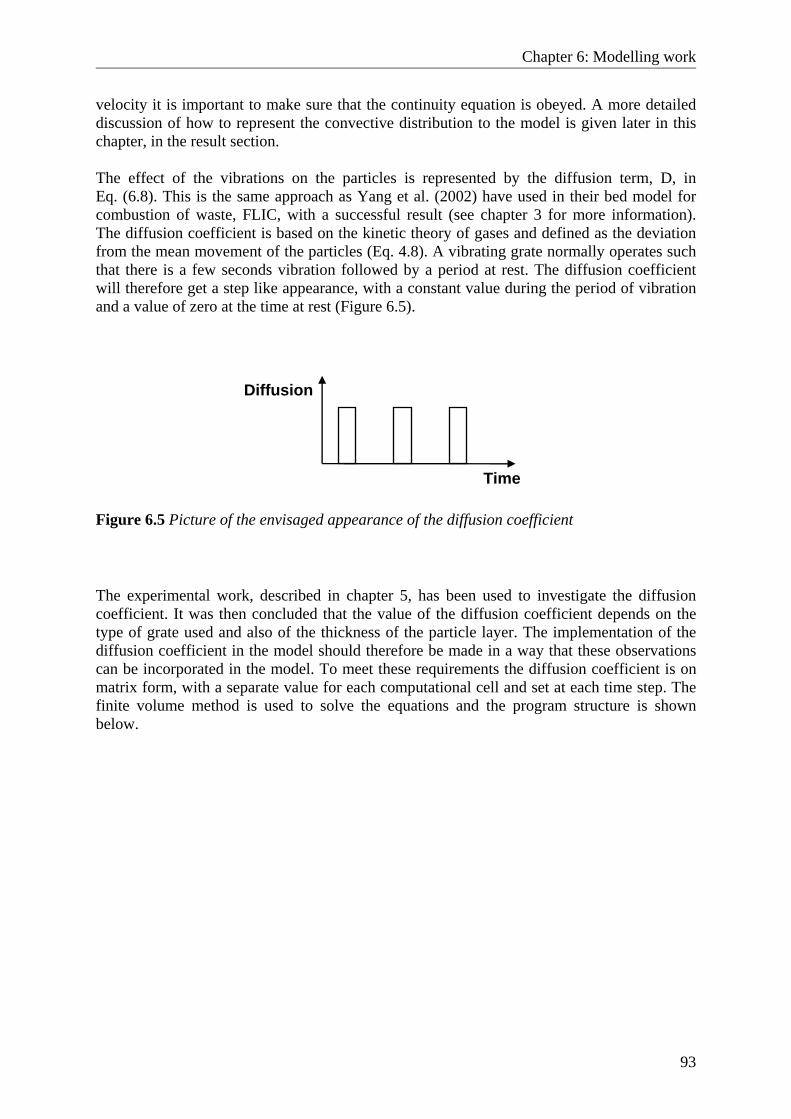
Chapter 6: Modelling work
93
velocity it is important to make sure that the continuity equation is obeyed. A more detailed discussion of how to represent the convective distribution to the model is given later in this chapter, in the result section. The effect of the vibrations on the particles is represented by the diffusion term, D, in Eq. (6.8). This is the same approach as Yang et al. (2002) have used in their bed model for combustion of waste, FLIC, with a successful result (see chapter 3 for more information). The diffusion coefficient is based on the kinetic theory of gases and defined as the deviation from the mean movement of the particles (Eq. 4.8). A vibrating grate normally operates such that there is a few seconds vibration followed by a period at rest. The diffusion coefficient will therefore get a step like appearance, with a constant value during the period of vibration and a value of zero at the time at rest (Figure 6.5).
Figure 6.5 Picture of the envisaged appearance of the diffusion coefficient
The experimental work, described in chapter 5, has been used to investigate the diffusion coefficient. It was then concluded that the value of the diffusion coefficient depends on the type of grate used and also of the thickness of the particle layer. The implementation of the diffusion coefficient in the model should therefore be made in a way that these observations can be incorporated in the model. To meet these requirements the diffusion coefficient is on matrix form, with a separate value for each computational cell and set at each time step. The finite volume method is used to solve the equations and the program structure is shown below.
Diffusion
Time
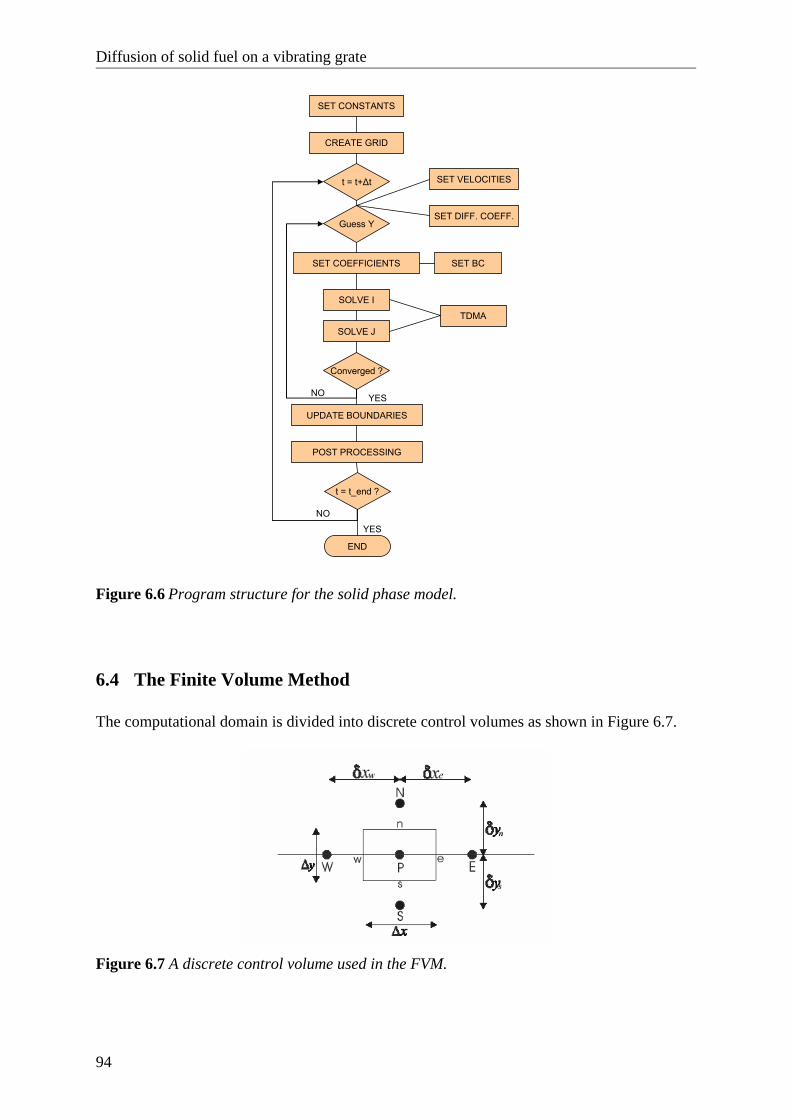
Diffusion of solid fuel on a vibrating grate
94
SET COEFFICIENTS
SOLVE I
t = t+Δt
SOLVE J
TDMA
SET BC
Converged ?
UPDATE BOUNDARIES
t = t_end ?
END
POST PROCESSING
CREATE GRID
SET CONSTANTS
Guess Y
SET VELOCITIES
SET DIFF. COEFF.
NO
NO
YES
YES
Figure 6.6 Program structure for the solid phase model.
6.4 The Finite Volume Method The computational domain is divided into discrete control volumes as shown in Figure 6.7.
Figure 6.7 A discrete control volume used in the FVM.
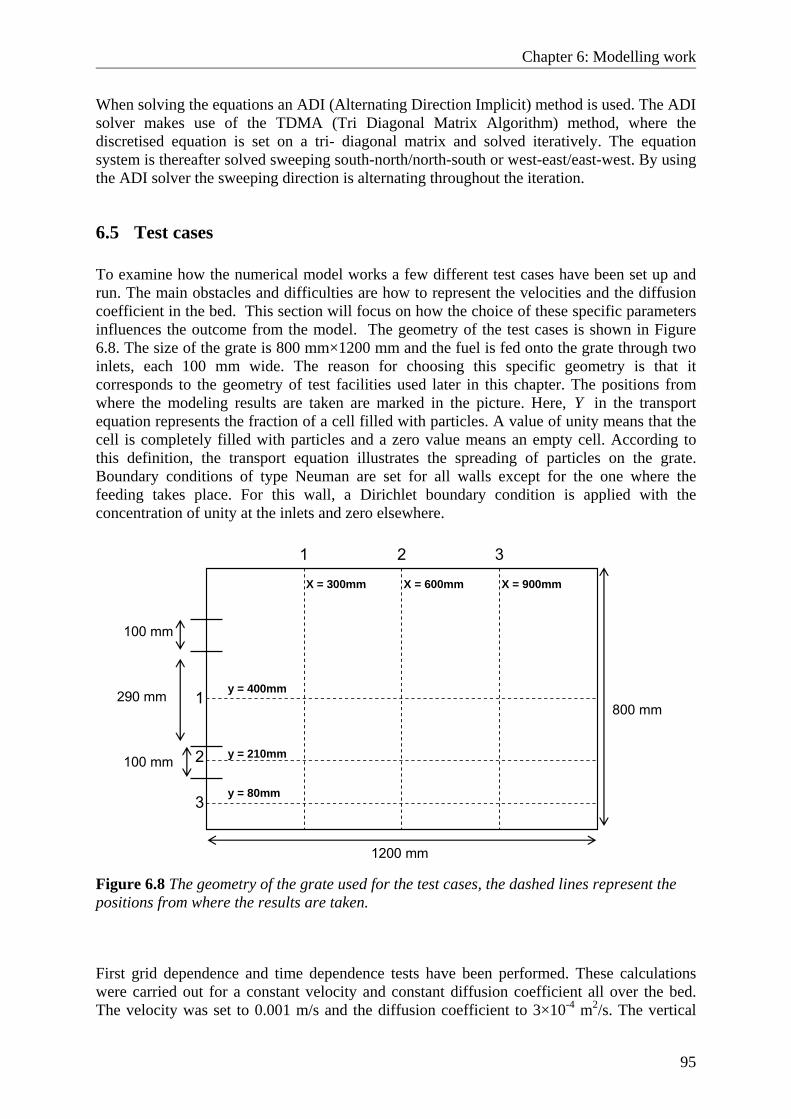
Chapter 6: Modelling work
95
When solving the equations an ADI (Alternating Direction Implicit) method is used. The ADI solver makes use of the TDMA (Tri Diagonal Matrix Algorithm) method, where the discretised equation is set on a tri- diagonal matrix and solved iteratively. The equation system is thereafter solved sweeping south-north/north-south or west-east/east-west. By using the ADI solver the sweeping direction is alternating throughout the iteration.
6.5 Test cases To examine how the numerical model works a few different test cases have been set up and run. The main obstacles and difficulties are how to represent the velocities and the diffusion coefficient in the bed. This section will focus on how the choice of these specific parameters influences the outcome from the model. The geometry of the test cases is shown in Figure 6.8. The size of the grate is 800 mm×1200 mm and the fuel is fed onto the grate through two inlets, each 100 mm wide. The reason for choosing this specific geometry is that it corresponds to the geometry of test facilities used later in this chapter. The positions from where the modeling results are taken are marked in the picture. Here, Y in the transport equation represents the fraction of a cell filled with particles. A value of unity means that the cell is completely filled with particles and a zero value means an empty cell. According to this definition, the transport equation illustrates the spreading of particles on the grate. Boundary conditions of type Neuman are set for all walls except for the one where the feeding takes place. For this wall, a Dirichlet boundary condition is applied with the concentration of unity at the inlets and zero elsewhere.
1200 mm
800 mm
100 mm
100 mm
290 mm
1 32
1
2
3
X = 300mm X = 600mm X = 900mm
y = 210mm
y = 80mm
y = 400mm
Figure 6.8 The geometry of the grate used for the test cases, the dashed lines represent the positions from where the results are taken.
First grid dependence and time dependence tests have been performed. These calculations were carried out for a constant velocity and constant diffusion coefficient all over the bed. The velocity was set to 0.001 m/s and the diffusion coefficient to 3×10⁻⁴ m2/s. The vertical
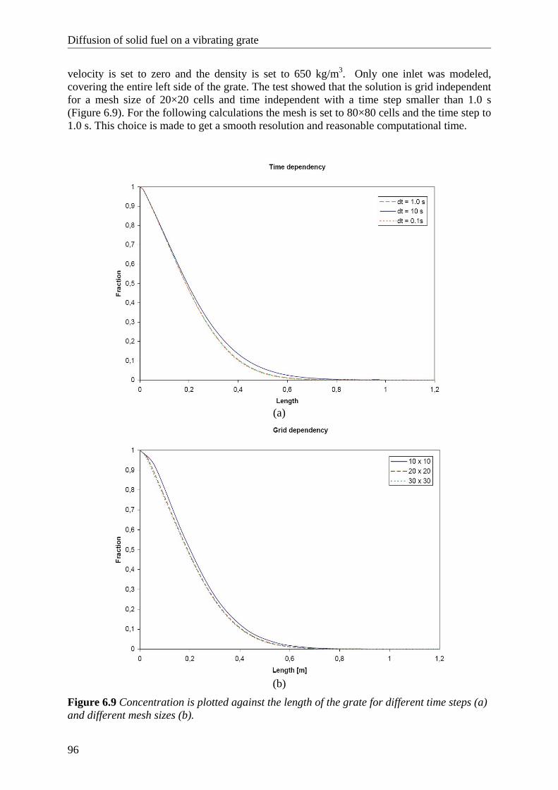
Diffusion of solid fuel on a vibrating grate
96
velocity is set to zero and the density is set to 650 kg/m3. Only one inlet was modeled, covering the entire left side of the grate. The test showed that the solution is grid independent for a mesh size of 20×20 cells and time independent with a time step smaller than 1.0 s (Figure 6.9). For the following calculations the mesh is set to 80×80 cells and the time step to 1.0 s. This choice is made to get a smooth resolution and reasonable computational time.
(a)
(b)
Figure 6.9 Concentration is plotted against the length of the grate for different time steps (a) and different mesh sizes (b).
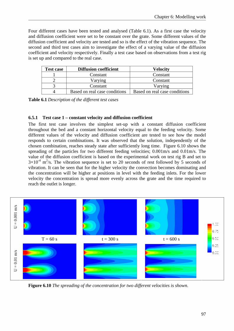
Chapter 6: Modelling work
97
Four different cases have been tested and analysed (Table 6.1). As a first case the velocity and diffusion coefficient were set to be constant over the grate. Some different values of the diffusion coefficient and velocity are tested and so is the effect of the vibration sequence. The second and third test cases aim to investigate the effect of a varying value of the diffusion coefficient and velocity respectively. Finally a test case based on observations from a test rig is set up and compared to the real case.
Test case Diffusion coefficient Velocity 1 Constant Constant 2 Varying Constant 3 Constant Varying 4 Based on real case conditions Based on real case conditions
Table 6.1 Description of the different test cases
6.5.1 Test case 1 – constant velocity and diffusion coefficient The first test case involves the simplest set-up with a constant diffusion coefficient throughout the bed and a constant horizontal velocity equal to the feeding velocity. Some different values of the velocity and diffusion coefficient are tested to see how the model responds to certain combinations. It was observed that the solution, independently of the chosen combination, reaches steady state after sufficiently long time. Figure 6.10 shows the spreading of the particles for two different feeding velocities; 0.001m/s and 0.01m/s. The value of the diffusion coefficient is based on the experimental work on test rig B and set to 3×10⁻⁴ m2/s. The vibration sequence is set to 20 seconds of rest followed by 5 seconds of vibration. It can be seen that for the higher velocity the convection becomes dominating and the concentration will be higher at positions in level with the feeding inlets. For the lower velocity the concentration is spread more evenly across the grate and the time required to reach the outlet is longer.
U =
0.0
01 m
/s
T = 60 s t = 300 s t = 600 s
U =
0.0
1 m
/s
Figure 6.10 The spreading of the concentration for two different velocities is shown.
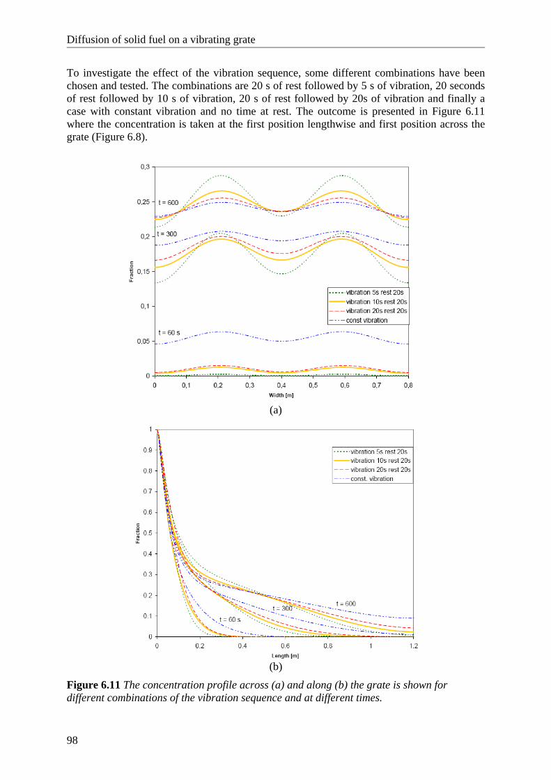
Diffusion of solid fuel on a vibrating grate
98
To investigate the effect of the vibration sequence, some different combinations have been chosen and tested. The combinations are 20 s of rest followed by 5 s of vibration, 20 seconds of rest followed by 10 s of vibration, 20 s of rest followed by 20s of vibration and finally a case with constant vibration and no time at rest. The outcome is presented in Figure 6.11 where the concentration is taken at the first position lengthwise and first position across the grate (Figure 6.8).
(a)
(b)
Figure 6.11 The concentration profile across (a) and along (b) the grate is shown for different combinations of the vibration sequence and at different times.
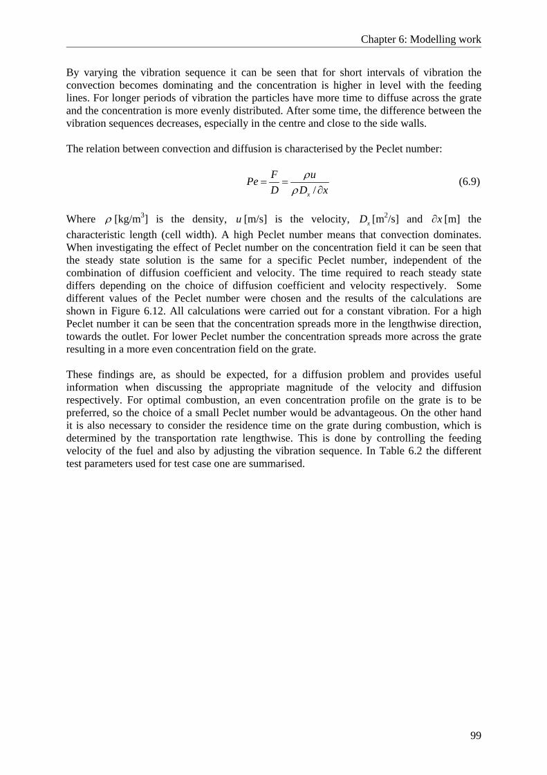
Chapter 6: Modelling work
99
By varying the vibration sequence it can be seen that for short intervals of vibration the convection becomes dominating and the concentration is higher in level with the feeding lines. For longer periods of vibration the particles have more time to diffuse across the grate and the concentration is more evenly distributed. After some time, the difference between the vibration sequences decreases, especially in the centre and close to the side walls. The relation between convection and diffusion is characterised by the Peclet number:
/x
F uPeD D x
ρρ
= =∂
(6.9)
Where ρ [kg/m3] is the density, u [m/s] is the velocity, xD [m2/s] and x∂ [m] the characteristic length (cell width). A high Peclet number means that convection dominates. When investigating the effect of Peclet number on the concentration field it can be seen that the steady state solution is the same for a specific Peclet number, independent of the combination of diffusion coefficient and velocity. The time required to reach steady state differs depending on the choice of diffusion coefficient and velocity respectively. Some different values of the Peclet number were chosen and the results of the calculations are shown in Figure 6.12. All calculations were carried out for a constant vibration. For a high Peclet number it can be seen that the concentration spreads more in the lengthwise direction, towards the outlet. For lower Peclet number the concentration spreads more across the grate resulting in a more even concentration field on the grate. These findings are, as should be expected, for a diffusion problem and provides useful information when discussing the appropriate magnitude of the velocity and diffusion respectively. For optimal combustion, an even concentration profile on the grate is to be preferred, so the choice of a small Peclet number would be advantageous. On the other hand it is also necessary to consider the residence time on the grate during combustion, which is determined by the transportation rate lengthwise. This is done by controlling the feeding velocity of the fuel and also by adjusting the vibration sequence. In Table 6.2 the different test parameters used for test case one are summarised.
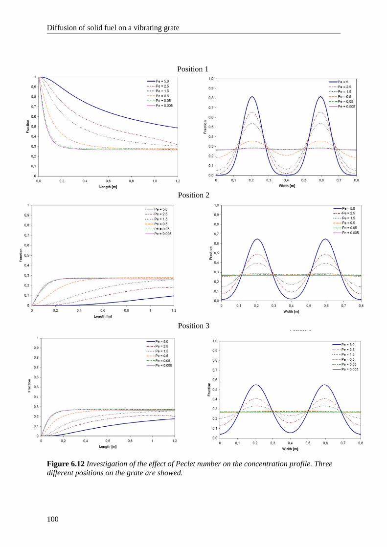
Diffusion of solid fuel on a vibrating grate
100
Position 1
Position 2
Position 3
Figure 6.12 Investigation of the effect of Peclet number on the concentration profile. Three different positions on the grate are showed.
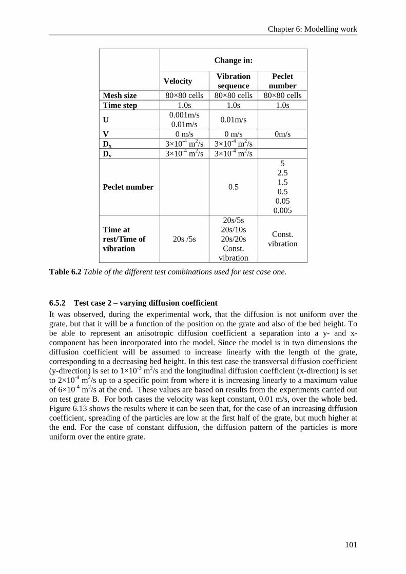
Chapter 6: Modelling work
101
Change in:
Velocity Vibration
sequence Peclet
number Mesh size 80×80 cells 80×80 cells 80×80 cells Time step 1.0s 1.0s 1.0s
U 0.001m/s 0.01m/s 0.01m/s
V 0 m/s 0 m/s 0m/s Dx 3×10⁻⁴ m2/s 3×10⁻⁴ m2/s Dy 3×10⁻⁴ m2/s 3×10⁻⁴ m2/s
Peclet number 0.5
5 2.5 1.5 0.5 0.05 0.005
Time at rest/Time of vibration
20s /5s
20s/5s 20s/10s 20s/20s Const.
vibration
Const. vibration
Table 6.2 Table of the different test combinations used for test case one.
6.5.2 Test case 2 – varying diffusion coefficient It was observed, during the experimental work, that the diffusion is not uniform over the grate, but that it will be a function of the position on the grate and also of the bed height. To be able to represent an anisotropic diffusion coefficient a separation into a y- and x- component has been incorporated into the model. Since the model is in two dimensions the diffusion coefficient will be assumed to increase linearly with the length of the grate, corresponding to a decreasing bed height. In this test case the transversal diffusion coefficient (y-direction) is set to 1×10⁻³ m2/s and the longitudinal diffusion coefficient (x-direction) is set to 2×10⁻⁴ m2/s up to a specific point from where it is increasing linearly to a maximum value of 6×10⁻⁴ m2/s at the end. These values are based on results from the experiments carried out on test grate B. For both cases the velocity was kept constant, 0.01 m/s, over the whole bed. Figure 6.13 shows the results where it can be seen that, for the case of an increasing diffusion coefficient, spreading of the particles are low at the first half of the grate, but much higher at the end. For the case of constant diffusion, the diffusion pattern of the particles is more uniform over the entire grate.
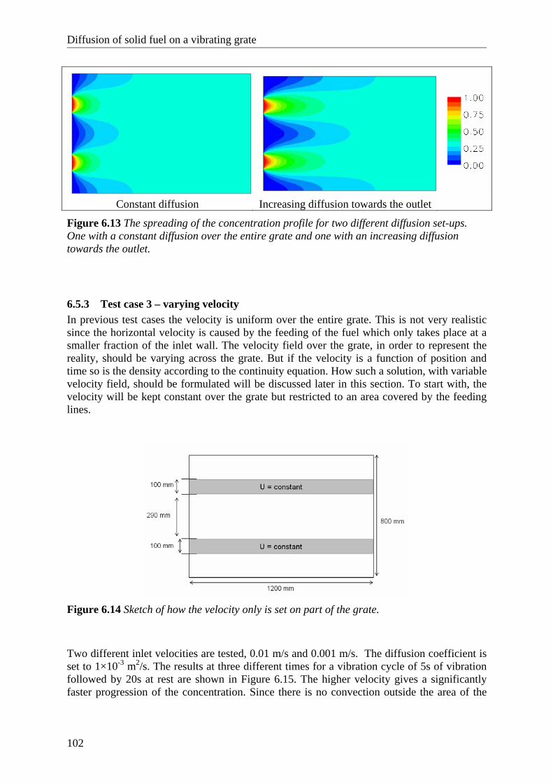
Diffusion of solid fuel on a vibrating grate
102
Constant diffusion Increasing diffusion towards the outlet
Figure 6.13 The spreading of the concentration profile for two different diffusion set-ups. One with a constant diffusion over the entire grate and one with an increasing diffusion towards the outlet.
6.5.3 Test case 3 – varying velocity In previous test cases the velocity is uniform over the entire grate. This is not very realistic since the horizontal velocity is caused by the feeding of the fuel which only takes place at a smaller fraction of the inlet wall. The velocity field over the grate, in order to represent the reality, should be varying across the grate. But if the velocity is a function of position and time so is the density according to the continuity equation. How such a solution, with variable velocity field, should be formulated will be discussed later in this section. To start with, the velocity will be kept constant over the grate but restricted to an area covered by the feeding lines.
Figure 6.14 Sketch of how the velocity only is set on part of the grate.
Two different inlet velocities are tested, 0.01 m/s and 0.001 m/s. The diffusion coefficient is set to 1×10⁻³ m2/s. The results at three different times for a vibration cycle of 5s of vibration followed by 20s at rest are shown in Figure 6.15. The higher velocity gives a significantly faster progression of the concentration. Since there is no convection outside the area of the
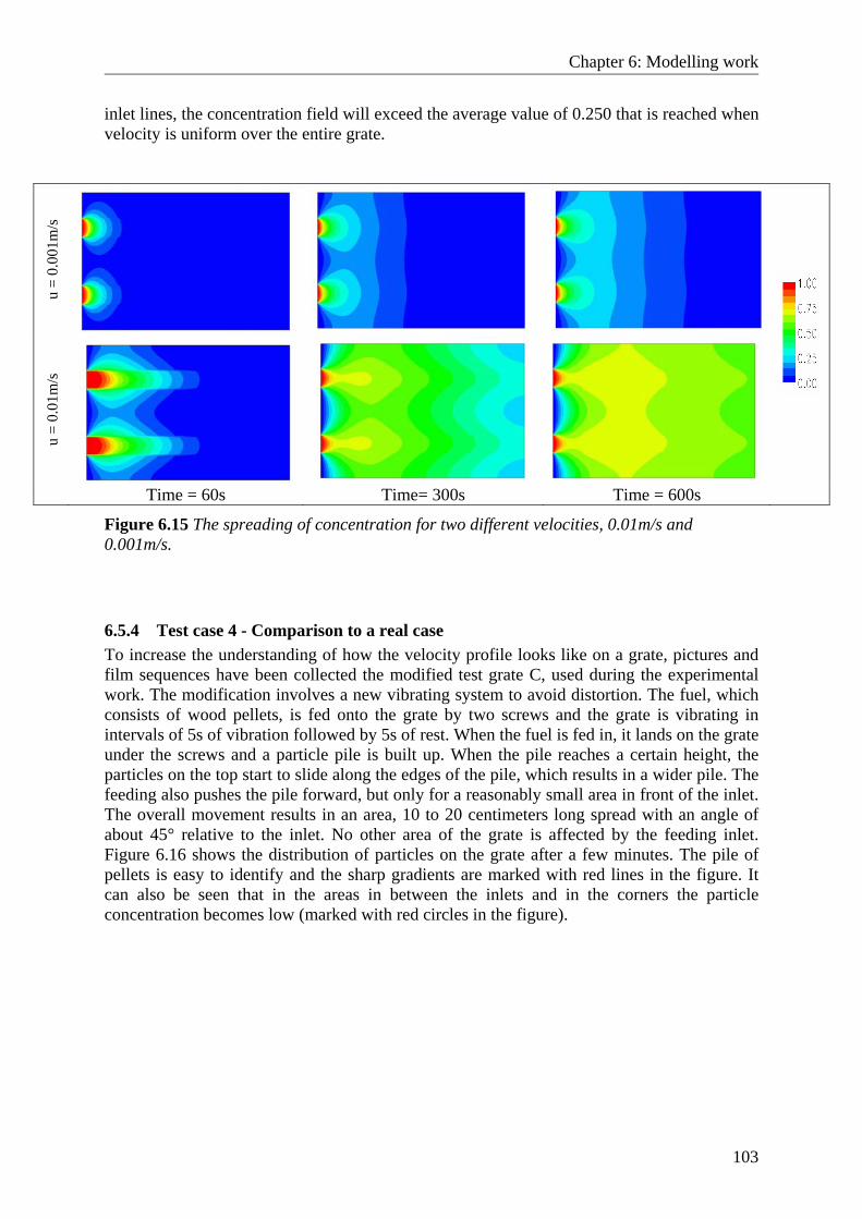
Chapter 6: Modelling work
103
inlet lines, the concentration field will exceed the average value of 0.250 that is reached when velocity is uniform over the entire grate.
u =
0.00
1m/s
u =
0.01
m/s
Time = 60s Time= 300s Time = 600s
Figure 6.15 The spreading of concentration for two different velocities, 0.01m/s and 0.001m/s.
6.5.4 Test case 4 - Comparison to a real case To increase the understanding of how the velocity profile looks like on a grate, pictures and film sequences have been collected the modified test grate C, used during the experimental work. The modification involves a new vibrating system to avoid distortion. The fuel, which consists of wood pellets, is fed onto the grate by two screws and the grate is vibrating in intervals of 5s of vibration followed by 5s of rest. When the fuel is fed in, it lands on the grate under the screws and a particle pile is built up. When the pile reaches a certain height, the particles on the top start to slide along the edges of the pile, which results in a wider pile. The feeding also pushes the pile forward, but only for a reasonably small area in front of the inlet. The overall movement results in an area, 10 to 20 centimeters long spread with an angle of about 45° relative to the inlet. No other area of the grate is affected by the feeding inlet. Figure 6.16 shows the distribution of particles on the grate after a few minutes. The pile of pellets is easy to identify and the sharp gradients are marked with red lines in the figure. It can also be seen that in the areas in between the inlets and in the corners the particle concentration becomes low (marked with red circles in the figure).
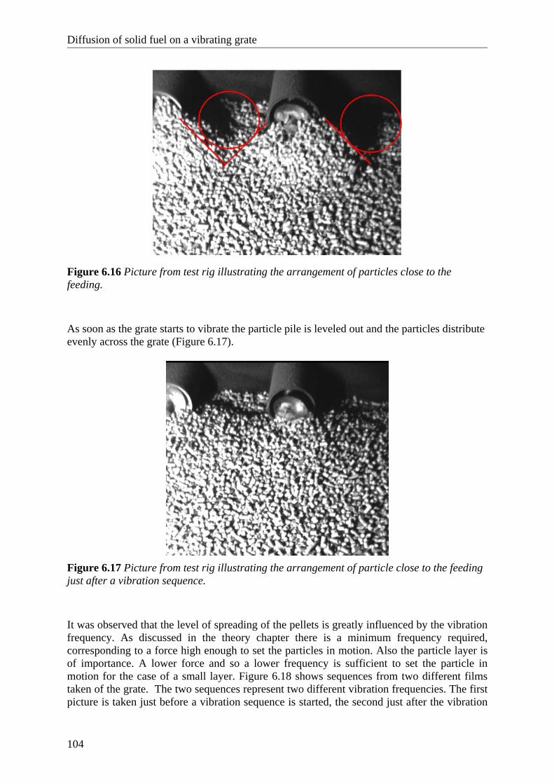
Diffusion of solid fuel on a vibrating grate
104
Figure 6.16 Picture from test rig illustrating the arrangement of particles close to the feeding.
As soon as the grate starts to vibrate the particle pile is leveled out and the particles distribute evenly across the grate (Figure 6.17).
Figure 6.17 Picture from test rig illustrating the arrangement of particle close to the feeding just after a vibration sequence.
It was observed that the level of spreading of the pellets is greatly influenced by the vibration frequency. As discussed in the theory chapter there is a minimum frequency required, corresponding to a force high enough to set the particles in motion. Also the particle layer is of importance. A lower force and so a lower frequency is sufficient to set the particle in motion for the case of a small layer. Figure 6.18 shows sequences from two different films taken of the grate. The two sequences represent two different vibration frequencies. The first picture is taken just before a vibration sequence is started, the second just after the vibration
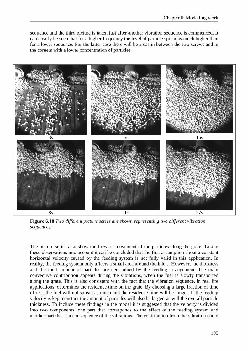
Chapter 6: Modelling work
105
sequence and the third picture is taken just after another vibration sequence is commenced. It can clearly be seen that for a higher frequency the level of particle spread is much higher than for a lower sequence. For the latter case there will be areas in between the two screws and in the corners with a lower concentration of particles.
3s 5s 15s
8s 10s 27s
Figure 6.18 Two different picture series are shown representing two different vibration sequences.
The picture series also show the forward movement of the particles along the grate. Taking these observations into account it can be concluded that the first assumption about a constant horizontal velocity caused by the feeding system is not fully valid in this application. In reality, the feeding system only affects a small area around the inlets. However, the thickness and the total amount of particles are determined by the feeding arrangement. The main convective contribution appears during the vibrations, when the fuel is slowly transported along the grate. This is also consistent with the fact that the vibration sequence, in real life applications, determines the residence time on the grate. By choosing a large fraction of time of rest, the fuel will not spread as much and the residence time will be longer. If the feeding velocity is kept constant the amount of particles will also be larger, as will the overall particle thickness. To include these findings in the model it is suggested that the velocity is divided into two components, one part that corresponds to the effect of the feeding system and another part that is a consequence of the vibrations. The contribution from the vibration could
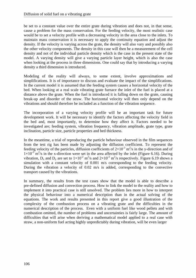
Diffusion of solid fuel on a vibrating grate
106
be set to a constant value over the entire grate during vibration and does not, in that sense, cause a problem for the mass conservation. For the feeding velocity, the most realistic case would be to set a velocity profile with a decreasing velocity in the area close to the inlets. To maintain mass conservation it is necessary to apply the continuity equation and adjust the density. If the velocity is varying across the grate, the density will also vary and possibly also the other velocity components. The density in this case will then be a measurement of the cell density and not of the individual particle density which is the case in the present state of the model. A varying density will give a varying particle layer height, which is also the case when looking at the process in three dimensions. One could say that by introducing a varying density a third dimension is introduced. Modeling of the reality will always, to some extent, involve approximations and simplifications. It is of importance to discuss and evaluate the impact of the simplifications. In the current model it is assumed that the feeding system causes a horizontal velocity of the bed. When looking at a real scale vibrating grate furnace the inlet of the fuel is placed at a distance above the grate. When the fuel is introduced it is falling down on the grate, causing break-up and disorder of the straw. The horizontal velocity will then only depend on the vibrations and should therefore be included as a function of the vibration sequence. The incorporation of a varying velocity profile will be an important task for future development work. It will be necessary to identify the factors affecting the velocity field in the bed and, most importantly, to determine how they affect it. Factors needed to be investigated are; feeding system, vibration frequency, vibration amplitude, grate type, grate inclination, particle size, particle properties and bed thickness. In the meantime, a trial of reproducing the particle behaviour observed in the film sequences from the test rig has been made by adjusting the diffusion coefficient. To represent the feeding velocity of the particles, diffusion coefficients of 2×10⁻³ m2/s in the y-direction and of 1×10⁻³ m2/s in the x-direction were set in the area affected by the inlet (Figure 6.16). During vibration, Dx and Dy are set to 1×10⁻² m2/s and 2×10⁻² m2/s respectively. Figure 6.19 shows a simulation with a constant velocity of 0.001 m/s corresponding to the feeding velocity. During the vibration a velocity of 0.02 m/s is added, corresponding to the convective transport caused by the vibrations. In summary, the results from the test cases show that the model is able to describe a pre-defined diffusion and convection process. How to link the model to the reality and how to implement it into practical case is still unsolved. The problem lies more in how to interpret the physical behaviour into a numerical description than in the actual solving of the equations. The work and results presented in this report give a good illustration of the complexity of the combustion process on a vibrating grate and the difficulties in the numerical description of the process. Even with a uniform fuel like wood pellets and with combustion omitted, the number of problems and uncertainties is fairly large. The amount of difficulties that will arise when deriving a mathematical model applied to a real case with straw, a non-uniform fuel acting highly unpredictably during vibration, will be even larger
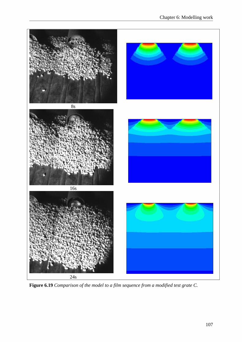
Chapter 6: Modelling work
107
8s
16s
24s
Figure 6.19 Comparison of the model to a film sequence from a modified test grate C.
Diffusion of solid fuel on a vibrating grate
108
6.6 Future work The future work, that has to be performed to develop a complete bed model, will be to extend the model into three dimensions and to include the combustion process. Below follows a brief discussion of how this work could be carried out.
6.6.1 Three dimensions A restriction of the simulations presented is that they are carried out in two dimensions. However, the extension to a three dimensional model is straightforward. How to implement the velocity and diffusion is not as obvious. It is necessary to add a vertical component that will have a strong dependency on the vibration. Theory shows that the diffusion is greater in the direction of the vibration which in this case is the vertical direction. It is therefore adequate to assume that the diffusion coefficient in the vertical direction should be larger than in the other two directions. The horizontal diffusion coefficient will depend on the vertical position in the bed, but also on the total bed height at the specific location on the grate. If combustion was added the situation becomes even more complex since the bed height will also depend on the conversion process. To implement this theory into the model, further investigation and experimental work are needed.
6.6.2 Combustion A vital step in the bed model development will be to incorporate the combustion process. Straw particles are a convenient type of fuel to model in the sense that they can be considered as thermally thin (low Biot number). This simplifies the modeling work since no consideration to internal temperature gradients needs to be taken. When incorporating the chemical reactions the time scales will be of importance. The time scales of the combustion will be on a different level compared to the case where only diffusion takes place. This will be of importance when choosing the time step. As discussed previously, the combustion process certainly also determines the bed height. The reactions are normally taken into account by introducing source terms in the transports equations. Another change, when introducing combustion, is that the energy equation for both solid and gas phases needs to be solved.
Chapter 7: Conclusion and Perspectives
109
7 Conclusion and Perspectives
The purpose of this work has been to develop a bed model for combustion of straw on a vibrating grate. Focus has been on investigating how to represent the macroscopic transportation of fuel on the grate. However, when studying the literature of mixing theory and vibration of granular flow, several conclusions can be adapted for the conditions of a vibrating grate:
• Vibration is anisotropic, with the highest contribution in the direction of the vibrations
• The degree of diffusion is dependent on bed height, particle size and properties
• The diffusion depends on the frequency and amplitude of vibration
Straw, both pelletised and untreated, differ from granular material both in size and packing structure. Despite these discrepancies the overall behaviour is of the same kind and has been taken into consideration when developing the bed model. The similarities in the particle behaviour were shown by the experimental work carried out within this project with the main results being:
• Diffusion increases linearly with increasing frequency and amplitude.
• Diffusion increases linearly with decreasing particle layer thickness.
• Dx and Dy are of the same order of magnitude.
A problem during the experimental work has been to construct a test rig that can give a smooth acceleration curve. The vibration level required to rearrange for example wood pellets is fairly high, which places a high stress on the grate construction. Three different test rigs have been used, each with a unique vibration pattern and rig design, in order to investigate the diffusion behaviour of the particles. The results showed a very high dependency on the rig design. This is an important outcome, since it shows that a diffusion coefficient has to be determined for each type of grate to be modeled, and that this cannot be generalized without resorting to a semi-empirical approach.
Diffusion of solid fuel on a vibrating grate
110
Most existing bed models do not take particle mixing into account. For a vibrating grate it is clear that the mixing and transportation of the fuel are of great significance in order to obtain an accurate description of the conversion process on the grate. The model approach chosen in this work has been to separate the gas and solid phases into two independent models related to each other through the bed porosity. By treating the bed as a porous media and using Ergun’s equation for the gas flow, the numerical work is simplified and the computational time shortened. The effect of the choice of how to represent the velocity and diffusion coefficients in the model has been investigated. The main results and conclusions from the modeling work are:
• The model is able to accurately describe a predefined diffusion problem in two dimensions.
• The vibrations give rise to both a diffusive and convective contribution in the model. The mean velocity of the particles can be seen as a convective process whilst the deviation from the mean velocity should be treated as a diffusive process.
• In order to introduce a varying velocity depending on the position on the grate, a modification of the model is necessary where also the density will vary as a consequence of the continuity equation. The definition of the density will thereby change from being the particle density to be the cell density, i.e. a measure of how dense the particles are packed in each cell.
Measurements from straw-fired furnaces with vibrating grates show a high occurrence of unwanted CO peaks. When observing a real scale straw fired furnace it can be seen that the combustion behaviour is extremely chaotic and actually very far from deterministic. The straw particles are thrown upwards and around in an uncontrollable way during the vibrations. When fresh fuel as a consequence of the vibrations is exposed to oxygen an intensification of the combustion takes place and this might be one reason for the CO peaks identified in the over bed area. A recent IR recording of the grate of Enstedværket verifies this kind of behaviour. The IR recordings were made in conjunction to an optical measurement campaign carried out by Risø (Clausen, 2005). Two frame sequences, taken with 10s in-between, are shown in Figure 7.1 . The flow direction is towards the lower right corner of the picture, one of the measuring probes can be seen to the right.
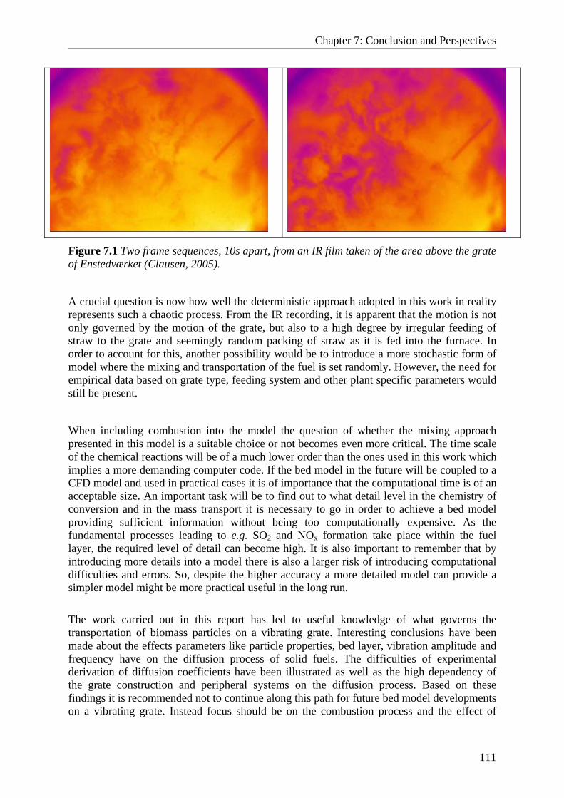
Chapter 7: Conclusion and Perspectives
111
Figure 7.1 Two frame sequences, 10s apart, from an IR film taken of the area above the grate of Enstedværket (Clausen, 2005).
A crucial question is now how well the deterministic approach adopted in this work in reality represents such a chaotic process. From the IR recording, it is apparent that the motion is not only governed by the motion of the grate, but also to a high degree by irregular feeding of straw to the grate and seemingly random packing of straw as it is fed into the furnace. In order to account for this, another possibility would be to introduce a more stochastic form of model where the mixing and transportation of the fuel is set randomly. However, the need for empirical data based on grate type, feeding system and other plant specific parameters would still be present.
When including combustion into the model the question of whether the mixing approach presented in this model is a suitable choice or not becomes even more critical. The time scale of the chemical reactions will be of a much lower order than the ones used in this work which implies a more demanding computer code. If the bed model in the future will be coupled to a CFD model and used in practical cases it is of importance that the computational time is of an acceptable size. An important task will be to find out to what detail level in the chemistry of conversion and in the mass transport it is necessary to go in order to achieve a bed model providing sufficient information without being too computationally expensive. As the fundamental processes leading to e.g. SO2 and NOx formation take place within the fuel layer, the required level of detail can become high. It is also important to remember that by introducing more details into a model there is also a larger risk of introducing computational difficulties and errors. So, despite the higher accuracy a more detailed model can provide a simpler model might be more practical useful in the long run.
The work carried out in this report has led to useful knowledge of what governs the transportation of biomass particles on a vibrating grate. Interesting conclusions have been made about the effects parameters like particle properties, bed layer, vibration amplitude and frequency have on the diffusion process of solid fuels. The difficulties of experimental derivation of diffusion coefficients have been illustrated as well as the high dependency of the grate construction and peripheral systems on the diffusion process. Based on these findings it is recommended not to continue along this path for future bed model developments on a vibrating grate. Instead focus should be on the combustion process and the effect of

Diffusion of solid fuel on a vibrating grate
112
mixing incorporated through a randomly given, or predefined diffusion coefficient. The challenging work of creating a bed model that in three dimensions accurately describes the burning process of straw on a vibrating grate and provides detailed input data for CFD modeling of the over-bed area still remains. This thesis acts like a mile stone in the bed modeling process and emphasizes the needs and challenges for continuous research work within the area.
Chapter 8: References
113
8 References Alves, S.S., Figueiredo, J.L. (1989). A model for pyrolysis of wet wood. Chemical Engineering Science, vol 44 no 12, 2861-2869.
Babcock &Wilcox Vølund. Retrieved 31 May 2007 from < http://www.volund.dk/ technologies_products/biomass_energy_systems/combustion_grates/ vibration_grate_hvb_water_cooled/illustrations_of_the_hvb_grate>.
Barker, G.C., Mehta, A. (1993). Transient phenomena, self-diffusion, and orientational effects in vibrated powders. Physical Review E, vol 47 no1_184-188.
Baxter, G.W., Behringer, R.P. (1990). Cellular automata models of granular flow. Physical Review A, 42 (2) 1017-1020.
Baxter, L, Coombes, P., Gifford, J., Guiu, G., Hourmann Jakobsen, H., Koppejan, J., Livingston, W., Logie, W., Nussbaumer, T., Obenberger, I., Oravainen, H., Schenkel, Y., Skreiberg, Ö., Tullin, C, van Loo, S. (2002). Handbook of Biomass Combustion and Co-firing. Twente University Press, Enschede, the Netherlands, ISBN 9036517737
Beckmann, M., Scholtz, R. (1995). Simplified mathematical model of combustion in stoker systems. Proceedings of the third European Conference on Industrial Furnaces and Boilers, 61-70.
Berry, M., Jensen, R. (2003). Investigation of diffusion on a vibrating bed. Semester 9 student project, Institute of Energy technology, Aalborg University, Denmark.
Bird, R.B., Stewart, W.E., Lightfoot., E. N. (2002). Transport Phenomena, second edition. John Wiley & Sons, Inc. ISBN 0-471-41077-2.
Bocquet, L., Losert, W., Schalk, D., Lubensky, T.C., Gollub, J.P. (2001). Granular shear flow dynamics and forces:Experiment and continuum theory. Physical review E. Volume 65, 011307
Borman, G.L., Ragland, K.W. (1998). Combustion Engineering. MCGraw-Hill, Singapore. ISBN 0-07-115978-9).
Brennen, C.E., Ghosh, S., Wassgren, C.R. (1996). Vertical oscillation of a bed of granular material. Journal of Applied Mechanics, vol 63:156-161.
Bruch, C., Peters, B., Nussbaumer, T. (2003) Modelling wood combustion under fixed bed conditions. Fuel 82:729-738.
Bryden, K., Ragland, K. (1996). Numerical Modeling of a Deep, Fixed Bed Combustor. Energy and Fuels 10, 269-275.
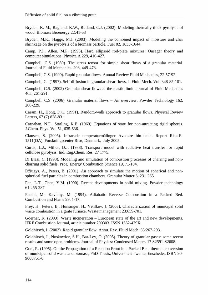
Diffusion of solid fuel on a vibrating grate
114
Bryden, K. M., Ragland, K.W., Rutland, C.J. (2002). Modeling thermally thick pyrolysis of wood. Biomass Bioenergy 22:41-53
Bryden, M.K., Hagge, M.J. (2003). Modeling the combined impact of moisture and char shrinkage on the pyrolysis of a biomass particle. Fuel 82, 1633-1644.
Camp, P.J., Allen, M.P. (1996). Hard ellipsoid rod-plate mixtures: Onsager theory and computer simulations. Physica A 229, 410-427.
Campbell, C.S. (1989). The stress tensor for simple shear flows of a granular material. Journal of Fluid Mechanics. 203, 449-473.
Campbell, C.S. (1990). Rapid granular flows. Annual Review Fluid Mechanics, 22:57-92.
Campbell, C. (1997). Self-diffusion in granular shear flows. J. Fluid Mech. Vol. 348-85-101.
Campbell, C.S. (2002) Granular shear flows at the elastic limit. Journal of Fluid Mechanics 465, 261-291.
Campbell, C.S. (2006). Granular material flows – An overview. Powder Technology 162, 208-229.
Caram, H., Hong, D.C. (1991). Random-walk approach to granular flows. Physical Review Letters, 67 (7) 828-831.
Carnahan, N.F., Starling, K.E. (1969). Equations of state for non-attracting rigid spheres. J.Chem. Phys. Vol 51, 635-636.
Clausen, S. (2005). Infrarøde temperaturmålinger Avedøre bio-kedel. Report Risø-R-1511(DA), Forskningscenter Risø, Denmark, July 2005.
Curtis, L.J., Miller, D.J. (1988). Transport model with radiative heat transfer for rapid cellulose pyrolysis. Ind. Eng.Chem. Res. 27 1775.
Di Blasi, C. (1993). Modeling and simulation of combustion processes of charring and non-charring solid fuels. Prog. Energy Combustion Science 19, 71-104.
Džiugys, A., Peters, B. (2001). An approach to simulate the motion of spherical and non-spherical fuel particles in combustion chambers. Granular Matter 3, 231-265.
Fan, L.T., Chen, Y.M. (1990). Recent developments in solid mixing. Powder technology 61:255-287
Fatehi, M., Kaviany, M. (1994). Adiabatic Reverse Combustion in a Packed Bed. Combustion and Flame 99, 1-17.
Frey, H., Peters, B., Hunsinger, H., Vehlkov, J. (2003). Characterization of municipal solid waste combustion in a grate furnace. Waste management 23:659-701.
Göerner, K. (2003). Waste incineration – European state of the art and new developments. IFRF Combustion Journal, article number 200303. ISSN 1562-479X.
Goldhirsch, I. (2003). Rapid granular flow. Annu. Rev. Fluid Mech. 35:267-293.
Goldhirsch, I., Noskowicz, S.H., Bar-Lev, O. (2005). Theory of granular gases: some recent results and some open problems. Journal of Physics: Condensed Matter. 17 S2591-S2608.
Gort, R. (1995). On the Propagation of a Reaction Front in a Packed Bed, thermal conversion of municipal solid waste and biomass, PhD Thesis, Universiteit Twente, Enschede,. ISBN 90-9008751-6.
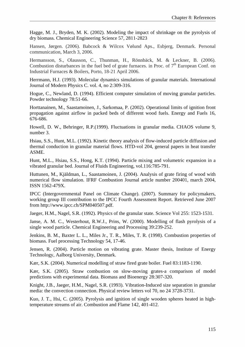
Chapter 8: References
115
Hagge, M. J., Bryden, M. K. (2002). Modeling the impact of shrinkage on the pyrolysis of dry biomass. Chemical Engineering Science 57, 2811-2823
Hansen, Jørgen. (2006). Babcock & Wilcox Vølund Aps., Esbjerg, Denmark. Personal communication, March 3, 2006.
Hermansson, S., Olausson, C., Thunman, H., Rönnbäck, M. & Leckner, B. (2006). Combustion disturbances in the fuel bed of grate furnaces. in Proc. of 7th European Conf. on Industrial Furnaces & Boilers, Porto, 18-21 April 2006.
Herrmann, H.J. (1993). Molecular dynamics simulations of granular materials. International Journal of Modern Physics C. vol. 4, no 2:309-316.
Hogue, C., Newland, D. (1994). Efficient computer simulation of moving granular particles. Powder technology 78:51-66.
Horttanainen, M., Saastamoinen, J., Sarkomaa, P. (2002). Operational limits of ignition front propagation against airflow in packed beds of different wood fuels. Energy and Fuels 16, 676-686.
Howell, D. W., Behringer, R.P.(1999). Fluctuations in granular media. CHAOS volume 9, number 3.
Hsiau, S.S., Hunt, M.L. (1992). Kinetic theory analysis of flow-induced particle diffusion and thermal conduction in granular material flows. HTD-vol 204, general papers in heat transfer ASME.
Hunt, M.L., Hsiau, S.S., Hong, K.T. (1994). Particle mixing and volumetric expansion in a vibrated granular bed. Journal of Fluids Engineering, vol.116:785-791.
Huttunen, M., Kjäldman, L., Saastamoinen, J. (2004). Analysis of grate firing of wood with numerical flow simulation. IFRF Combustion Journal article number 200401, march 2004, ISSN 1562-479X.
IPCC (Intergovernmental Panel on Climate Change). (2007). Summary for policymakers, working group III contribution to the IPCC Fourth Assessment Report. Retrieved June 2007 from http://www.ipcc.ch/SPM040507.pdf.
Jaeger, H.M., Nagel, S.R. (1992). Physics of the granular state. Science Vol 255: 1523-1531.
Janse, A. M. C., Westerhout, R.W.J., Prins, W. (2000). Modelling of flash pyrolysis of a single wood particle. Chemical Engineering and Processing 39:239-252.
Jenkins, B. M., Baxter L. L., Miles Jr., T. R., Miles, T. R. (1998). Combustion properties of biomass. Fuel processing Technology 54, 17-46.
Jensen, R. (2004). Particle motion on vibrating grate. Master thesis, Institute of Energy Technology, Aalborg University, Denmark.
Kær, S.K. (2004). Numerical modelling of straw fired grate boiler. Fuel 83:1183-1190.
Kær, S.K. (2005). Straw combustion on slow-moving grates-a comparison of model predictions with experimental data. Biomass and Bioenergy 28:307-320.
Knight, J.B., Jaeger, H.M., Nagel, S.R. (1993). Vibration-Induced size separation in granular media: the convection connection. Physical review letters vol 70, no 24 3728-3731.
Kuo, J. T., Hsi, C. (2005). Pyrolysis and ignition of single wooden spheres heated in high-temperature streams of air. Combustion and Flame 142, 401-412.
Diffusion of solid fuel on a vibrating grate
116
Lim, C.N., Goh, Y.R., Nasserzadeh, V., Swithenbank, J., Riccius, O. (2001). The modelling of solid mixing in municipal waste incinerators. Powder Technology 114, 89-95.
McKendry, P. (2002). Energy production from biomass (part 1): overview of biomass. Bioresource Technology 83, 37-46.
Melby, P., Vega Reyes, F., Prevost, A., Robertson, R., Kumar, P., Egolf, D.A., Urbach, J,S. (2005). The dynamics of thin vibrated granular layers. Journal of Physics:Condensed Matter 17, S2689-S2704.
Metcalf, T.H., Knight, J.B., Jaeger, M. (1997). Standing wave patterns in shallow beds of vibrated granular material. Physics A 236:202-210.
Natarajan, V.V.R., Hunt, M.L., Taylor, E.D. (1995). Local measurements of velocity fluctuations and diffusion coefficients for a granular material flow. J. Fluid Mech. Vol 304:1-25.
Nikolaisen, L. Nielsen, C., Larsen, M.G., Nielsen, V., Zielke, U., Kristensen, J.K., Holm-Christensen, B. (1998). Halm til energiformål, teknik-miljø-økonomi. Videncenter for Halm-og Flisfyring. ISBN 87-90074-16-5.
Perram, J.W., Wertheim, M.S., Lebowitz, J.L, Williams, G.O. (1984). Monte Carlo simulation of hard spheroids. Chemical Physics Letters 105 (3) 277-279.
Peters, B. (2003) Thermal conversion of solid fuels. WIT Press. Southampton, Boston.
Peters, B., Dziugys, A. (2002). Numerical simulation of the motion of granular material using object-oriented techniques. Computer methods in applied mechanics and engineering 191, 1983-2007.
Rönnbäck, M., Axell, M., Gustavsson, L. (2000). Combustion processes in a biomass fuel bed-Experimental results. Progress in Thermochemical Biomass Conversion 17-22 September, Tyrol, Austria.
Saastamoinen, J., Richard, J.R. (1996). Simultaneously drying and pyrolysis of solid fuel particles. Combustion and Flame 106:288-300.
Saastamoinen, J.J., Taipale, R., Horttanainen, M., Sarkomaa, P. (2000). Propagation of the Ignition Front in Beds of Wood Particles. Combustion and Flame 123:214-226.
Santamaria, J., Rückert, F.U., Förtsch, D., Sprich, J., Staiger, B., Berger, R., Schnell, U., Hein, K.R.G. (2002). Numerical simulation of a grate-firing-system for biomass. Proceedings of 6th European Conference on Industrial Furnaces and Boilers, Volume IV, Estoril-Lisboa, Portugal, April 02-05, 2002, 105-116.
Scharler, R., Obernberger, I. (2000). Numerical Modelling of Biomass Grate Furnaces. Proceedings of 5th European Conference on Industrial Furnaces and Boilers, Porto Portugal, 11-14 April.
Shin, D., Choi, S. (2000). The combustion of simulated waste particles in a fixed bed. Combust. Flame 121:167-180.
Tai, C.H., Hsiau, S.S. (2004). Dynamiv behaviours of powders in a vibrating bed. Powder technology 139:221-232.
Thomas, B., Mason, M.G., Liu, Y.A., Squires, A.M. (1989). Identifying states in shallow vibrated beds. Powder Technology 57 267-280.
Thoroddsen, S.T., Shen, A. Q. (2001). Granular jets. Physics of fluids volume 13, number 1.
Chapter 8: References
117
Thunman, H., Andersson, S., Bengtsson, P., Leckner, B., Palchonok, G. (2005a). Combustion Engineering. Course book from the Department of Energy Conversion, Chalmers University of Technology.
Thunman, H., Leckner, B. (2001). Ignition and propagation of a reaction front in cross-current bed combustion of wet biofuels. Fuel 80:473-81.
Thunman, H., Leckner, B. (2003). Co-current counter-current fixed bed combustion of biofuel- a comparison. Fuel 82 275-283.
Thunman, H., Leckner, B. (2005b). Influence of Size and Density of Fuel on Combustion in a Packed Bed. Proceedings of the combustion Institute volume 30, issue 2 January 2005 pp 2939-2946.
Thunman, H., Leckner, B., Niklasson, F., Johnsson, F. (2002). Combustion of Wood Particles-A Particle Model For Eulerian Calculations. Combustion and flame 129:30-46.
van den Broek, R., Faaij, A., Wijk, A. (1995). Biomass combustion -Power Generation Technologies. Energy from Biomass: an assessment of two promising systems for energy production, Background report 4.1. Department of Science, Technology and Society, Utrecht University, The Netherlands.
van der Lans, R.P., Pedersen, L.T., Jensen, A., Glarborg, P., Dam-Johansen, K. (2000). Modelling and experiments of straw combustion in a grate furnace. Biomass and Bioenergy 19:199-208.
Veijonen, K., Vainikka, P., Järvinen, T., Alakangas, E., VTT processes. (2003). Biomass co-firing an efficient way to reduce greenhouse gas emissions. European Bioenergy Network. Retrieved 01 June 2007 from <http://ec.europa.eu/energy/res/sectors/doc/ bioenergy/cofiring_eu_bionet.pdf>
Versteeg, H.K., Malalasekera, W. (1995). An Introducion to Computational Fluid Dynamics. Longman Group Ltd. ISBN 0-582-21884-5.
Wassgren, C.R., Brennen, C.E., Hunt, M.L. (1996). Vertical Vibration of a Deep Granular material in a container. Journal of Applied Mechanics, vol63:712-719.
Yanagida, T., Matchett, A.J., Coulthard, J.M. (2002). Effective mass of powder beds subjected to low magnitude vibration and its application to binary systems: Part1-experimental methodology. Chemical Engineering Science 57, 2653-2661.
Yang, S.C., Hsiau, S.S. (2001). Self-diffusion analysis in a vibrated granular bed. Advanced Powder Technology. Vol 12 No 1 66-77.
Yang, Y.B, Goh, Y.R., Zakaria, R., Nasserzadeh, V., Swithenbank, J. (2002). Mathematical modelling of MSW incineration on a travelling bed. Waste Management 22:369-380.
Yang, Y.B., Goodfellow, J., Nasserzadeh, V. (2005c). Study on the transient process of waste fuel incineration in a full scale moving-bed furnace. Combustion Science and Technology 177:127-150.
Yang, Y.B., Lim, C.N., Goodfellow, J., Sharifi, V.N., Swithenbank, J. (2005b). A diffusion model for particle mixing in a packed bed of burning solids. Fuel 84, 213-225.
Yang, Y. B., Ryu, C., Khor, A., Yates, N.E., Sharifi, V. (2005). Effect of fuel properties on biomass combustion. Part II. modelling approach-identification of the controlling factors. Fuel 84:2116-2130.
Diffusion of solid fuel on a vibrating grate
118
Yang, Y.B., Sharifi, V.N., Swithenbank, J. (2004). Effect of air flow rate and fuel moisture on the burning behaviours of biomass and simulated municipal solid wastes in packed beds. Fuel 83:1553-1562.
Yang, Y.B, Yamauchi, H., Nasserzadeh, V., Swithenbank, J. (2003a). Effect of moisture content in fuel on the combustion behaviour of biomass and municipal solid waste in a packed bed. J.I. Energy, Vol 76:105-115.
Yang, Y.B., Yamauchi, H., Nasserzadeh, V., Swithenbank, J. (2003b). Effects of fuel devolatilisation on the combustion of wood chips and incineration of simulated municipal solid wastes in a packed bed. Fuel 82, 2205-2221.
Yin, C. (2007). PSO 4792: Grate Firing of Biomass- Measurements, validation and demonstration. Project report for PSO 4792, Institute of Energy technology, Aalborg University, Denmark, April 2007.
Zakaria, R., Goh, Y.R., Yang, Y.B., Lim, C.N., Goodfellow, J., Chan, K.H., Reynolds, G., Ward, D., Siddall, R.G., Nasserzadeh, V., Swithenbank, J. (2000). Fundamentals Aspects of Emissions from the Burning Bed in a Municipal Solid Waste Incinerator. Proceedings from 5th European conference on industrial furnaces and boilers, Porto-Portugal, 11-14 April.
Zamankhan, P. (2004). Complex Flow Dynamics In Dense Granular Flows. Doctoral thesis, Lappeenranta University of Technology, Finland. ISBN 951-764-821-9.
Zhou, H., Jensen, A.D., Glarborg, P., Jensen, P.A., Kavaliauskas, A. (2005). A numerical modelling of straw combustion in a fixed bed. Fuel 84:389-403.
Zik, O., Stavans, J. (1991). Self diffusion in granular flows. Europhysics letter. Vol 14 issue 3 255-258.
Appendix A- The PIV method
119
Appendix A- The PIV method A.1 General description of PIV Particle Imaging Velocimetry (PIV) is a measurement technique for determining velocity fields. By measure the distance the particles have travelled in a known time interval the velocity can be calculated. To measure a flow velocity seeding particles are introduced into the flow. Different types of particles are chosen depending on the flow properties, since it is important that the particles follow the flow. A section of the flow field is illuminated by laser and the light is pulsating to freeze the movement of the seeding particles. The time in between the light pulses is then used to calculate the velocity. The distance traveled by the particles is obtained by detecting the position of the tracer particles by a CCD (Charged Coupled Device) camera. The pulsing light sheet and the camera are synchronised so that particles captured during light pulse one are registered in frame one, particles captured during light pulse two registered in frame two and so on. Each camera image is divided into a number of interrogation areas. For each interrogation area the image from the first and second light pulses is correlated to derive an average particle displacement vector. This is done for all interrogation areas which results in a vector map of all the particle displacements. The displacement is then divided by the known time interval between two pictures and a map of raw velocity vectors is thereby produced. Since PIV is an instantaneous measurement technique all information about the particle displacement is sampled at the same time and there is a statistical chance that there will be some regions with no realistic input. Therefore it is necessary to post process the obtained data and validate the vector maps. It is for this reason the vector maps from the correlation process normally are called raw-vector maps.
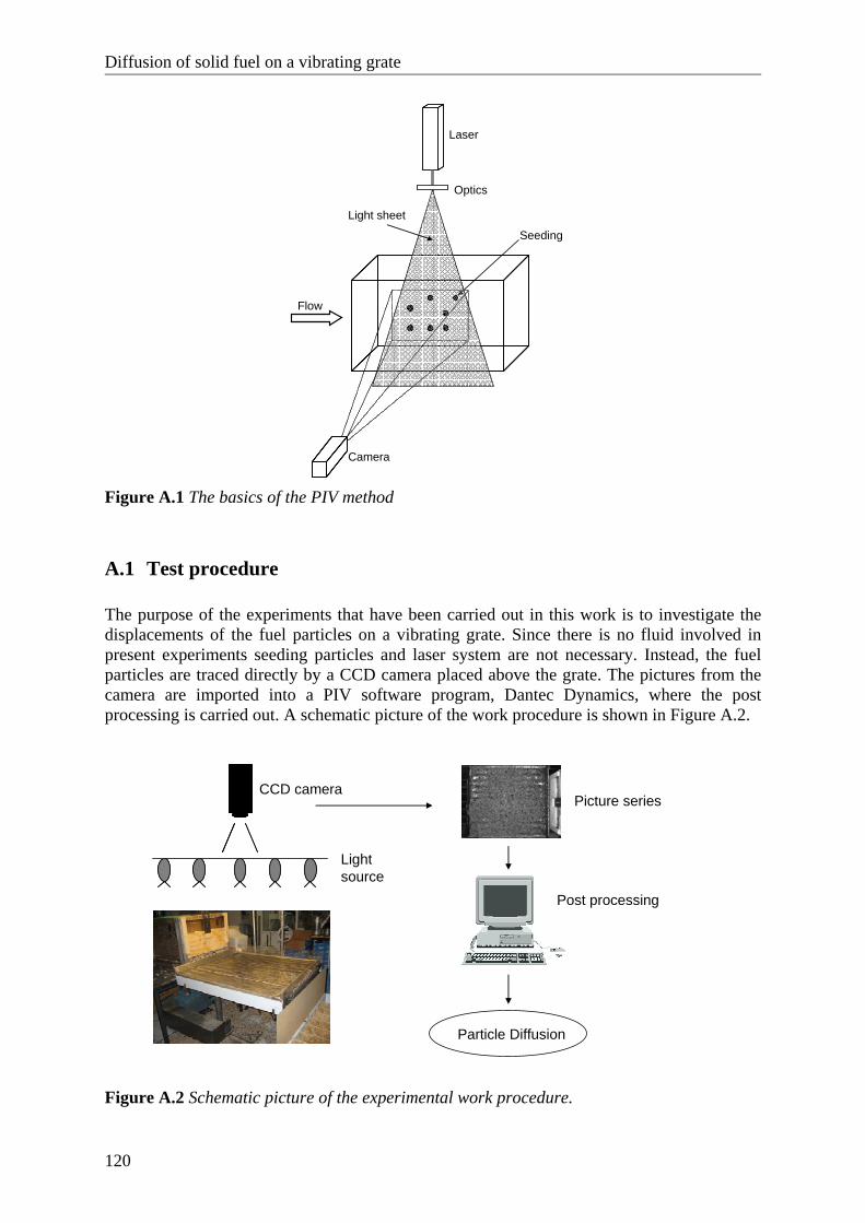
Diffusion of solid fuel on a vibrating grate
120
Camera
Seeding
Flow
Laser
Optics
Light sheet
Figure A.1 The basics of the PIV method
A.1 Test procedure The purpose of the experiments that have been carried out in this work is to investigate the displacements of the fuel particles on a vibrating grate. Since there is no fluid involved in present experiments seeding particles and laser system are not necessary. Instead, the fuel particles are traced directly by a CCD camera placed above the grate. The pictures from the camera are imported into a PIV software program, Dantec Dynamics, where the post processing is carried out. A schematic picture of the work procedure is shown in Figure A.2.
CCD camera
Post processing
Light source
Particle Diffusion
Picture series
Figure A.2 Schematic picture of the experimental work procedure.
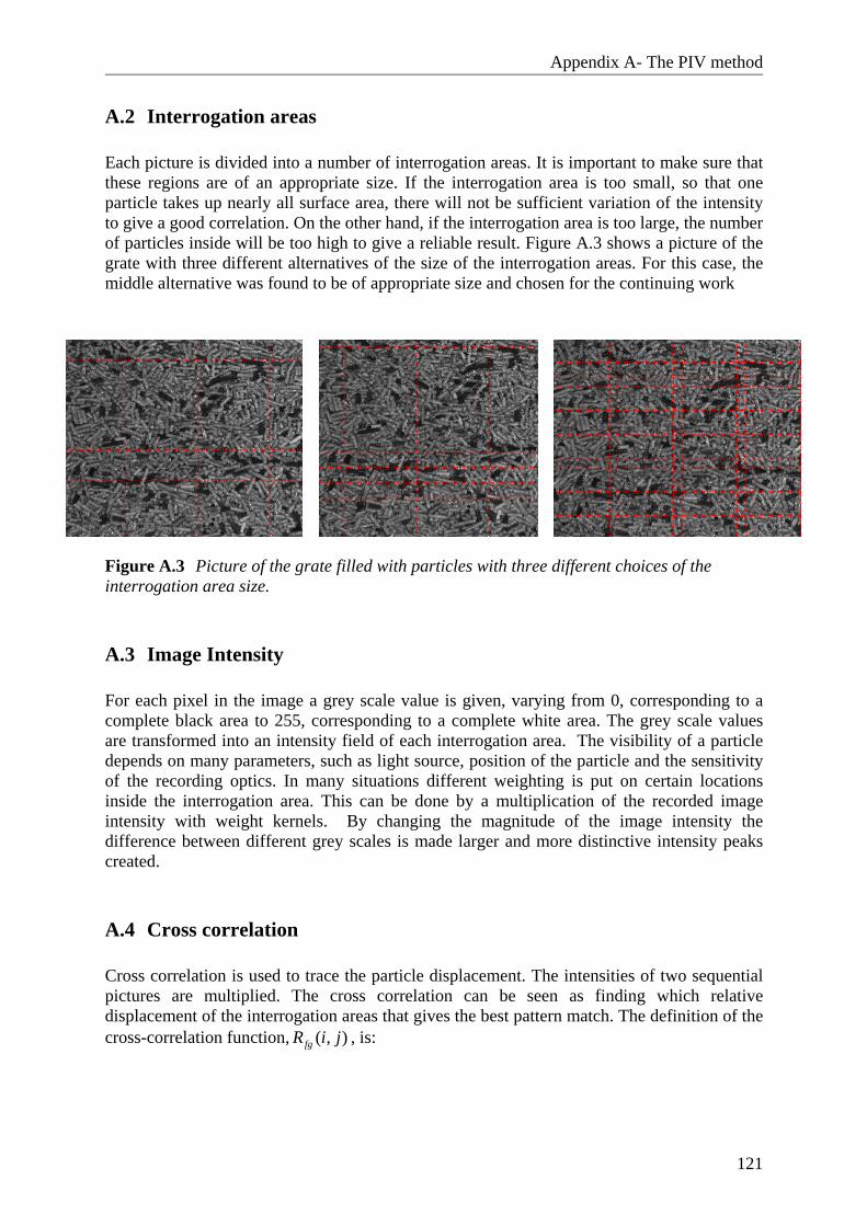
Appendix A- The PIV method
121
A.2 Interrogation areas Each picture is divided into a number of interrogation areas. It is important to make sure that these regions are of an appropriate size. If the interrogation area is too small, so that one particle takes up nearly all surface area, there will not be sufficient variation of the intensity to give a good correlation. On the other hand, if the interrogation area is too large, the number of particles inside will be too high to give a reliable result. Figure A.3 shows a picture of the grate with three different alternatives of the size of the interrogation areas. For this case, the middle alternative was found to be of appropriate size and chosen for the continuing work
Figure A.3 Picture of the grate filled with particles with three different choices of the interrogation area size.
A.3 Image Intensity For each pixel in the image a grey scale value is given, varying from 0, corresponding to a complete black area to 255, corresponding to a complete white area. The grey scale values are transformed into an intensity field of each interrogation area. The visibility of a particle depends on many parameters, such as light source, position of the particle and the sensitivity of the recording optics. In many situations different weighting is put on certain locations inside the interrogation area. This can be done by a multiplication of the recorded image intensity with weight kernels. By changing the magnitude of the image intensity the difference between different grey scales is made larger and more distinctive intensity peaks created.
A.4 Cross correlation Cross correlation is used to trace the particle displacement. The intensities of two sequential pictures are multiplied. The cross correlation can be seen as finding which relative displacement of the interrogation areas that gives the best pattern match. The definition of the cross-correlation function, ( , )fgR i j , is:
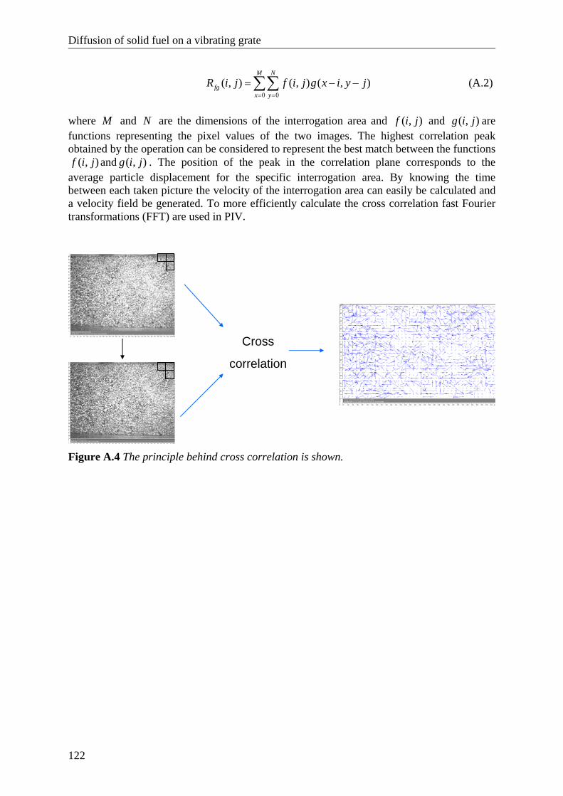
Diffusion of solid fuel on a vibrating grate
122
0 0
( , ) ( , ) ( , )M N
fgx y
R i j f i j g x i y j= =
= − −∑∑ (A.2)
where M and N are the dimensions of the interrogation area and ( , )f i j and ( , )g i j are functions representing the pixel values of the two images. The highest correlation peak obtained by the operation can be considered to represent the best match between the functions
( , )f i j and ( , )g i j . The position of the peak in the correlation plane corresponds to the average particle displacement for the specific interrogation area. By knowing the time between each taken picture the velocity of the interrogation area can easily be calculated and a velocity field be generated. To more efficiently calculate the cross correlation fast Fourier transformations (FFT) are used in PIV.
Cross
correlation
Figure A.4 The principle behind cross correlation is shown.