Embed Size (px)
Citation preview

Predictive Modelling I
SML201: Introduction to Data Science, Spring 2020
Michael GuerzhoySome slides from Andrew Ng

Linear regression
2
Notation:
m = Number of training examplesx’s = “input” variable / featuresy’s = “output” variable / “target” variable
Size in feet2 (x) Price ($) in 1000's (y)
𝑥(1) = 2104 𝑦(1) =460
𝑥(2) =1416 𝑦(2) =232
𝑥(3) =1534 𝑦(2) =315
𝑥(4) = 852 𝑦(2) =178… …
Training set ofhousing prices(Portland, OR)

3
0
125000
250000
375000
500000
0 750 1500 2250 3000
0
125000
250000
375000
500000
0 750 1500 2250 3000
Housing Prices(Portland, OR)
Price(in 1000s of
dollars)
Size (feet2)
• Equation for the “best” green line: price = 𝑎0 + 𝑎1𝑆𝑖𝑧𝑒• Prediction for a new size 𝑥: 𝑝𝑟𝑖𝑐𝑒 𝑥 = 𝑎0 + 𝑎1𝑥• We take “best” to mean that on average, our predictions are not far off

Cost functions
• If the correct price is 𝑦(𝑖) and we predicted
𝑎0 + 𝑎1𝑥 𝑖 , we are off by
|𝑦 𝑖 − 𝑎𝑜 + 𝑎1𝑥 𝑖 | (“error”)
• If we square this quantity, we still have a measure of how far off we are
𝑦 𝑖 − 𝑎𝑜 + 𝑎1𝑥 𝑖2
(“squared error”)
• Overall, we will be off (in terms of squared errors) by
𝑖=1
𝑚
𝑦 𝑖 − 𝑎𝑜 + 𝑎1𝑥 𝑖2
4

Simple Linear Regression
• Find the 𝑎0 and 𝑎1 such that
σ𝑖=1𝑚 𝑦 𝑖 − 𝑎𝑜 + 𝑎1𝑥 𝑖
2is as small as possible
• Graphically, roughly corresponds to “draw the best line through the scatterplot”
5

Multiple Linear Regression
• n quantities per case
• Find 𝑎0, 𝑎1, … , 𝑎𝑛 such that
σ𝑖=1𝑚 𝑦 𝑖 − 𝑎𝑜 + 𝑎1𝑥1
𝑖+ 𝑎2𝑥2
𝑖+ ⋯ + 𝑎𝑛𝑥𝑛
𝑖2
is small
6
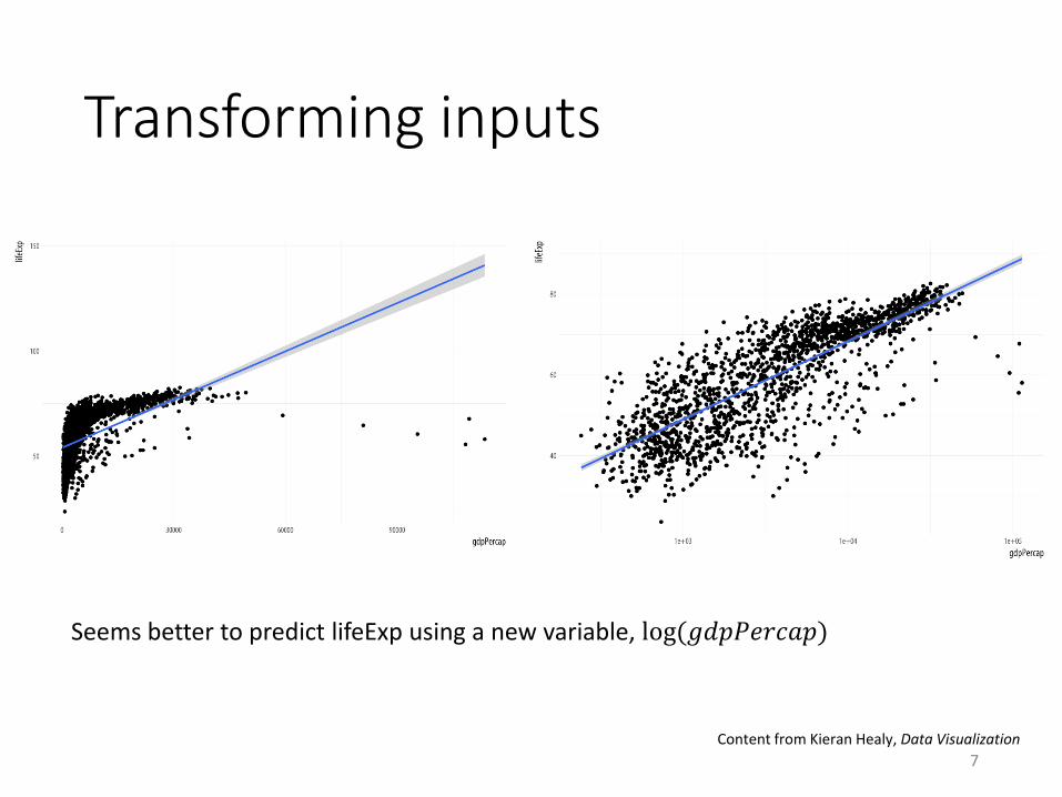
Transforming inputs
7
Seems better to predict lifeExp using a new variable, log(𝑔𝑑𝑝𝑃𝑒𝑟𝑐𝑎𝑝)
Content from Kieran Healy, Data Visualization

(switch to R)
8

Categorical variables
• Quantitative variables are numbers• Number, size, or weight of something• If x = 19 and x = 21 make sense, likely x = 20 would make
sense too• Discrete variables (e.g., counts) are still treated as
quantitative
• Categorical variables indicate categories• Country, Continent, …• Cannot put continents on a single scale
• Variables that could be either categorical or continuous: Likert scale response, color, …
9

Predicting with categorical variables• Suppose we are trying to predict 𝑦 using one categorical
variable (e.g., continent) which has k possible categories (e.g., 𝐶𝑜𝑛1, 𝐶𝑜𝑛2, …, 𝐶𝑜𝑛5)
• 𝑦(𝑖) ≈ 𝑎1,0 + 𝑎1,1𝐼𝑖,1 + 𝑎1,2𝐼𝑖,2 + ⋯ + 𝑎1,𝑘−1𝐼𝑖,𝑘−1
• 𝐼𝑖,1 = ቊ1, 𝑖𝑓 𝑡ℎ𝑒 𝑖 − 𝑡ℎ 𝑟𝑜𝑤 𝑐𝑜𝑛𝑡𝑎𝑖𝑛𝑠 𝐶𝑜𝑛1
0, 𝑜𝑡ℎ𝑒𝑟𝑤𝑖𝑠𝑒
• 𝐼𝑖,2 = ቊ1, 𝑖𝑓 𝑡ℎ𝑒 𝑖 − 𝑡ℎ 𝑟𝑜𝑤 𝑐𝑜𝑛𝑡𝑎𝑖𝑛𝑠𝐶𝑜𝑛2
0, 𝑜𝑡ℎ𝑒𝑟𝑤𝑖𝑠𝑒
• …
• Note: if the i-th point is 𝐶𝑜𝑛𝑡𝑘, then the prediction is 𝑎0• Potentially different predictions for each continent, despite the fact
that we didn’t include 𝐼𝑖,𝑘
10

(Switch to R)
11

Titanic Survival Case Study
• The RMS Titanic• British passenger liner
• Collided with an iceberg during her maiden voyage
• 2224 people aboard, 710 survived
• People on board• 1st class, 2nd class, 3rd class passengers (price of ticker +
social class played a role)
• Different ages, genders
12
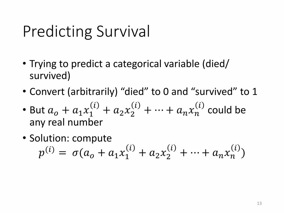
Predicting Survival
• Trying to predict a categorical variable (died/ survived)
• Convert (arbitrarily) “died” to 0 and “survived” to 1
• But 𝑎𝑜 + 𝑎1𝑥1𝑖
+ 𝑎2𝑥2𝑖
+ ⋯ + 𝑎𝑛𝑥𝑛𝑖
could be any real number
• Solution: compute
𝑝(𝑖) = 𝜎(𝑎𝑜 + 𝑎1𝑥1𝑖
+ 𝑎2𝑥2𝑖
+ ⋯ + 𝑎𝑛𝑥𝑛𝑖
)
13

Logistic function
• 𝜎 𝑦 =1
1+exp(−𝑦)
Inputs can be in (−∞, ∞), outputs will always be in (0, 1)
14

Logistic regression: prediction
𝑝(𝑖) = 𝜎(𝑎𝑜 + 𝑎1𝑥1𝑖
+ 𝑎2𝑥2𝑖
+ ⋯ + 𝑎𝑛𝑥𝑛𝑖
)
• 0 < 𝑝(𝑖) < 1
• Interpret 𝑝(𝑖) as the probability that the variable that we are predicting (i.e., 𝑦(𝑖)) is 1• For now, think of a probability is a number between 0
and 1 where 0 indicates that the event will not happen and 1 indicates that the event will happen.
15

(Switch to R)
16

Logistic regression: cost function
• For linear regression, we had
𝑖=1
𝑚
𝑦 𝑖 − 𝑎𝑜 + 𝑎1𝑥1𝑖
+ 𝑎2𝑥2𝑖
+ ⋯ + 𝑎𝑛𝑥𝑛𝑖
2
= 𝑖=1
𝑚
𝑦 𝑖 − 𝑝𝑟𝑒𝑑(𝑥𝑖
)2
• The cost is small if the predictions are close to the actual 𝑦’s
• For logistic regression:
−
𝑖
(𝑦 𝑖 log 𝑝 𝑖 + 1 − 𝑦 𝑖 log(1 − 𝑝 𝑖 ))
• Idea: the cost is small if the 𝑝’s are close to the 𝑦’s
• Won’t go into detail here
17