Predictive Modeling in Automobile Insurance 7-1-05 Modeling in Automobile... · 1 Predictive Modeling in Automobile Insurance: A Preliminary Analysis Stephen P. D’Arcy Abstract

Predictive Modeling in Automobile Insurance: A Preliminary Analysis

by

Stephen P. D’Arcy

Paper to be Presented at the

World Risk and Insurance Economics Congress

Salt Lake City, Utah

August 2005

Contact information:

Stephen P. D’Arcy Professor of Finance College of Business University of Illinois 1206 S. Sixth Street Champaign, IL 61820 Telephone: 217-333-0772 E-mail: [email protected]

1

Predictive Modeling in Automobile Insurance:

A Preliminary Analysis

Stephen P. D’Arcy

Abstract

This project applies the Data to Knowledge (D2K) systems developed by NCSA to the

Detail Claim Database (DCD) of the Automobile Insurers Bureau of Massachusetts to generate

predictive models to enhance insurance claim investigation practices. Data mining is a relatively

new tool for insurance companies. However, advances in applications of data mining have been

hindered by the lack of research that can be shared within the industry. Although insurers have

conducted many data mining projects for a variety of applications, including underwriting, rating

and claim investigation, they have generally resisted disclosing the details of this research in an

attempt to maintain a competitive advantage. In many cases, when insurers have tried to utilize

the results of these studies in their operations they have encountered regulatory resistance due to

a lack of full disclosure of the supporting documentation. This project seeks to redress some of

the problems limiting the advance of data mining and predictive modeling in the insurance

industry by conducting a study that can be shared within the industry and all the details can be

published. This study provides a significant advance over the few prior studies that used this

data set by utilizing the state-of-the-art data mining tools developed at NCSA.

This project examines the data set for patterns of claim behavior based on the records of

the almost one-half million automobile bodily injury claims included in the DCD. An updated

D2K system has been applied to these data to establish which factors can be effectively utilized

in the claims process in order to generate a predictive model to help insurers identify which

claims are most likely to generate cost savings by investigating the claim more extensively in an

attempt to deter fraudulent claiming behavior.

2

Overview

Technological advances have allowed the insurance industry to begin to apply data

mining techniques to the vast data bases the industry routinely collects in the course of

conducting its business. Data mining has been effectively used to determine significant

characteristics for use in underwriting applicants, to support the use of credit score factors in

rating, and to identify claims that should be investigated for fraudulent activity. Many insurers

have undertaken data mining projects, several consulting firms have established specialty areas

to develop predictive models based on data mining activity for insurers, and a cottage industry of

companies performing analytics and predictive modeling for insurance companies and other

industries has developed. Predictive modeling appears to represent a significant new avenue for

the insurance industry.

Several problems, though, need to be addressed before data mining can be applied most

effectively within the insurance industry. First, despite the extensive efforts by a large number

of parties, there have been very few published results of these studies. As one professional

colleague (who asked not to be identified) commented,

“Unfortunately, insurance companies are very sensitive and reluctant in sharing their data. I have done data mining and predictive modeling for the last 10 years, and have worked with more than 20 different clients. But none of them is willing to share the data publicly. For every project I have worked on so far, we have always signed an agreement with the clients that we cannot use the data for other purposes, not even for research.” Companies know the value they can obtain from data mining their information, and do

not want to lose this competitive advantage by giving away the results of their work. While this

is understandable behavior, its near universal application has prevented this area from advancing

to its full potential. By conducting each project separately, there is no benefit gained from the

experience of other companies. By requiring each project to stand on its own, subtle interactions

3

that are not significant based on a single study would be ignored, even though they might be

considered relevant if the results of numerous analyses could be combined.

A second problem is that the studies are performed by a small group of experts, and

shared with a small group of customers. This drastically limits the understanding of data mining

and predictive modeling to only a subset of the people who could actually benefit from these

techniques and unnecessarily limits the situations to which they will be applied. If most

individuals within an insurance company are not aware of data mining techniques, they will not

realize the potential applications of this technology to their everyday work. If the impetus for

data mining is for an expert to discover the application, and then convince a practitioner that a

large enough benefit can be obtained to justify the initial cost of a project, most potential

applications will not be addressed. However, if the results of data mining projects in one

company, or in one part of a company, can be disseminated, then other applications will become

obvious. This would advance the pace and productivity of this research.

A function of the limited sharing of data mining applications is the over reliance on a

specialized jargon appropriate for this field. Since most data mining research is shared only with

other specialists, if at all, then the terminology does not need to be understood by a wider

audience. Thus, even when data mining results are shared, the terminology restricts the

understanding of the results, or even the significance of the approach, to other experts.

Finally, one special attribute of the insurance industry is its regulatory structure.

Insurance is one of the most heavily regulated industries in this country. Insurers must obtain

regulatory approval for a wide variety of functions, including policy forms, rates, investments,

and underwriting and sales practices. If an insurer wants to use a specific characteristic in setting

rates, in many cases it must convince a regulator that this is an appropriate factor. Currently,

4

credit scoring is a particularly sensitive issue in many regulatory jurisdictions. Through data

mining insurance companies have found that certain personal characteristics that are related to

credit score are also related to insurance claims experience. In some cases regulators are

allowing these factors to be used; in others they are not. One element contributing to the

problems is that insurers and the modeling companies want to keep the results of their data

mining confidential. This confidentiality leads to misunderstandings and incorrect conclusions

about the effect of including credit scoring on certain segments of the population.

In this project we apply the data mining techniques developed by NCSA to insurance data

from the Automobile Insurers’ Bureau of Massachusetts. This data set is described by Derrig

(2003):

“The Detail Claim Database (DCD) is mandated by the Commissioner of Insurance for use by all companies operating in Massachusetts. It includes reports from all Massachusetts automobile bodily injury claims closing January 1, 1994 and subsequent. The DCD receives in excess of 160,000 claims filed annually and contains information not normally reported in insurance statistics, including injury information and related treatment expense statistics for medical and legal providers. The DCD is a progressive and unique creation of the Governing Committee of the Automobile Insurers Bureau of Massachusetts, and it is unparalleled in its level of detail and overall participation by any data collection effort elsewhere in the country. This system is viewed as a new cornerstone in the battle against insurance fraud in Massachusetts.” The most important feature of the DCD is that the results of research on this data set can

be freely shared by researchers, leading to cooperative advances in the development of predictive

models. This data set has been made available to a limited number of researchers and has been

the basis for several previous applications of data mining [Brockett, Derrig, Golden, Levine and

Alpert (2002), Derrig and Weisberg (2003), Tennyson and Salas-Forn (2002) and Viaene,

Derrig, Baesens and Dedene (2002)]. This sharing has led to collaboration and advances in this

field.

5

NCSA has developed a state-of-the-art data mining application process termed Data To

Knowledge (D2K) [Hsu, Welge, Redman and Clutter (2002)]. This system has been applied in a

number of business applications, including insurance. A recent innovation is an updated version

of this program that is designed to be user-friendly for the less technical practitioner. This

advance should be extremely helpful for this project, which seeks to make insurance data mining

techniques both more widely applicable and more easily understandable.

Literature Review

The prior published research using the Massachusetts claim database has focused on

several specific aspects of this data. Brockett, Xia and Derrig (1998) apply a feature mapping

process to classify potential fraud cases in bodily injury claims. Tennyson and Salsas-Form

(2002) look at a small sample of claims to determine if auditing was used primarily for detection

of fraud or deterrence of future fraud. Derrig and Weisberg (2003), in their most recent study

using the DCD, report on the results of an experiment to provide fraud indicators generated from

data mining to claim investigators to determine if that information leads to more effective

detection of fraudulent claims. Brockett, Derrig, Golden, Levine and Alpert (2002) apply

principal component analysis of RIDIT scores to automobile insurance claims. Viaene, Derrig,

Baesens and Dedene (2002) compare several binary classification techniques to automobile

insurance claims to determine which approach is most effective, but find no single method works

best.

6

Massachusetts Detail Claim Database

This database, mandated by the Commissioner of Insurance, consists of all automobile

bodily injury claims closing on or after January 1, 1994. The Automobile Insurers Bureau (AIB)

of Massachusetts maintains this database, which is accessible for all member companies of the

AIB. The database provided for this research consists of 491,591 claim observations with 95

variables from five categories included:

1. Policy Information 2. Claim Information

a. Accident date b. Report date c. Type of injury d. Type of treatment

3. Outpatient Medical Provider Information (up to 2 providers) a. Provider type (Medical Doctor, Medical Organization, Medical Institution,

Chiropractor, Chiropractic Organization, Physical Therapist, Physical Therapy Organization, N/A)

b. Amount billed c. Amount paid (PIP or BI)

4. Attorney Information 5. Claim Handling Information

a. Type of investigation i. Independent Medical Exam (IME) ii. Medical Audit (MA) iii. Special Investigation (SI)

b. Result of Investigation i. No change recommended ii. Billing or treatment curtailed iii. Damages mitigated iv. No show (the claimant failed to show up for an IME) v. Refused (the claimant refused to have an IME) vi. Claim denied (as the result of an SI) vii. Claim compromised (a compromise was worked out after an SI)

c. Amount of Savings Estimated from Each Type of Investigation

There are several recognized shortcomings of the DCD. The amounts listed for savings

from investigations are based on formulae that likely understate the full value of any savings

achieved, especially regarding bodily injury coverage. The type of medical provider is omitted

7

in many cases. Investigations undertaken and second outpatient medical provider information

are considered to be underreported. These problems are typical of most data mining studies, and

underscore the importance of accurate data for this type of research.

For the purpose of this research, the database was randomly divided into two

components, a training dataset of 400,000 observations and a testing dataset of 91,591

observations. Based on the training database, of the three types of investigations, IMEs were the

most common (16.72%), followed by MAs (11.02%) and then SIs (4.17%). The average

estimated savings from each type of investigation is $348.71 for Independent Medical Exams

(IME_SAVE), $367.08 for Medical Audits (MA_SAVE) and $1805.39 for Special

Investigations (SI_SAVE). These values for savings do not consider the cost of the investigation

itself.

Empirical Results

Initial Indicators Study by the D2K Decision Tree tool

1. Motivation – To test the relationship between the independent nominal (dummy)

variables and three dependent variables, IME_SAVE, MA_SAVE and SI_SAVE.

2. Methodology and Tools - Decision Tree and D2K Itinerary for Decision Tree

3. Approach - Dependent variables were taken as IME_Saved, MA_Saved and SI_Saved.

Independent variables are 7 out of 52 nominal variables. They were Policy Type,

Coverage, Em_Treat, Health_I, Injury Type, MP1_Type and MP2_Type. All other

nominal variables are either location, ID numbers or investigation information.

The possible values for all selected variables are listed as follows:

8

• Policy Type: P (personal) and C (commercial)

• Coverage: (BI), (U-1), (U-2) and (PIP/MED)

• Em_Treat: Y (Emergency and /or Inpatient Treatment or No Treatment – No Outpatient

Treatment), N (Out Patient Treatment Only) and B (Outpatient Treatment and Emergency

and /or Inpatient Treatment)

• Health_I: Y (Yes), N (No) and U (Unknown)

• Injury Type: 1-22, 30 or 99 according to the different types of injury.

• MP1_Type: MD, MO, MI, CH, CO, PT, PO and N/A.

• MP2_Type: Same as above

The D2K decision tree itinerary was applied separately for each of the seven selected

nominal variables. The whole dataset includes 491,591 observations, which were randomly

separated into 400,000 observations for a training dataset and 91,591 observations to be used as a

testing dataset by the D2K decision tree itinerary. The training dataset was used to generate the

possible trees. The testing dataset was used to generate the external error for each of the possible

trees to select the best tree and the optimal depth (number of levels). The maximum depth of the

trees is the number of the nominal variables included, which in this case is two for the policy

type variable (personal/commercial) or eight for medical provider (seven types plus N/A). The

absolute difference of the estimated and actual value of each dependent variable tested was used

as the measure of the tree’s evaluator.

For each of these seven nominal variables, there are some missing data. The missing data

is treated as a random distribution, so the trees were generated from the available data without

9

considering the impact of any specific relationships between any of the nominal variables and the

likelihood of data to be omitted.

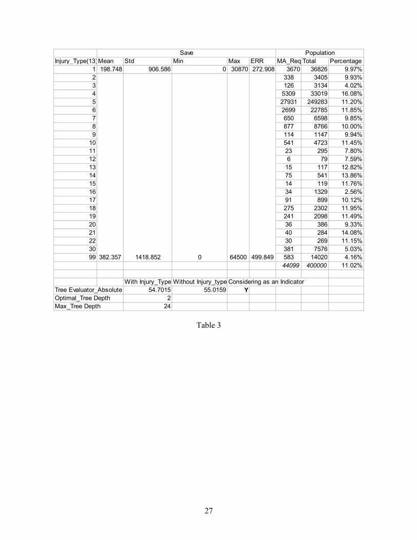
The decision tree results for the significant relationship between the selected dependent

and independent variables were summarized in the Table 1. Y indicates a significant relationship;

N indicates no significant relationship between the dependent variables and the selected nominal

variables.

Tables 2, 3 and 4 list the D2K decision tree results for the savings obtained through an

Independent Medical Exam (IME), Medical Audit (MA) and Special Investigation (SI)

considering the 24 different injury types. In Table 2, the 24 injury types are shown in the 1st

column. Each row provides the mean, standard deviation, minimum, maximum and the internal

error (D2K decision tree factor) for each injury type. The last three columns show the number of

IMEs that were requested for this injury type, the total number of claims with that injury type,

and the percentage of the claims for which an IME was requested (IME Requested/Total). Each

injury type is listed in a separate row, but some rows do not have any individual values for some

of the statistics. For these injury types, the D2K decision tree did not find a significant difference

to separate the injury types (in this case injury types 3,5,6,7,9,14,18,19) so they are combined

together as a group. For example, the value 351.289 is the mean savings for all these injury types

combined. At the bottom of Table 2, the external errors with and without the optimal tree are

listed as 93.379 and 93.5752. This means that if injury type were not used as an indicator of

potential savings from requesting an IME, then the error term would be 93.5752. This error

value was reduced to 93.379 by using the optimal tree based on injury type. The optimal decision

tree has a depth of 17 (16 individual injury types and the combined group of the 8 remaining

types), out of a potential tree depth of 24 (the total number of injury types). Injury type is a

10

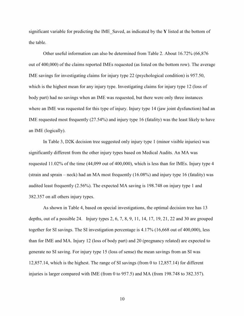
significant variable for predicting the IME_Saved, as indicated by the Y listed at the bottom of

the table.

Other useful information can also be determined from Table 2. About 16.72% (66,876

out of 400,000) of the claims reported IMEs requested (as listed on the bottom row). The average

IME savings for investigating claims for injury type 22 (psychological condition) is 957.50,

which is the highest mean for any injury type. Investigating claims for injury type 12 (loss of

body part) had no savings when an IME was requested, but there were only three instances

where an IME was requested for this type of injury. Injury type 14 (jaw joint dysfunction) had an

IME requested most frequently (27.54%) and injury type 16 (fatality) was the least likely to have

an IME (logically).

In Table 3, D2K decision tree suggested only injury type 1 (minor visible injuries) was

significantly different from the other injury types based on Medical Audits. An MA was

requested 11.02% of the time (44,099 out of 400,000), which is less than for IMEs. Injury type 4

(strain and sprain – neck) had an MA most frequently (16.08%) and injury type 16 (fatality) was

audited least frequently (2.56%). The expected MA saving is 198.748 on injury type 1 and

382.357 on all others injury types.

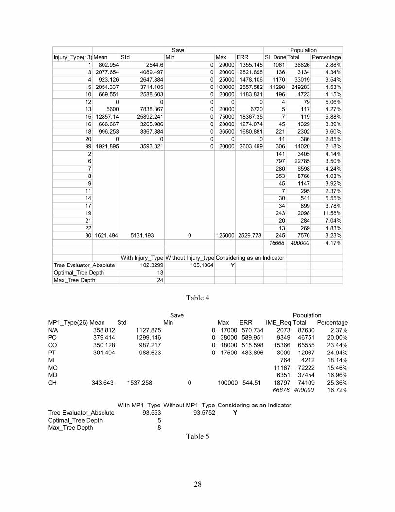
As shown in Table 4, based on special investigations, the optimal decision tree has 13

depths, out of a possible 24. Injury types 2, 6, 7, 8, 9, 11, 14, 17, 19, 21, 22 and 30 are grouped

together for SI savings. The SI investigation percentage is 4.17% (16,668 out of 400,000), less

than for IME and MA. Injury 12 (loss of body part) and 20 (pregnancy related) are expected to

generate no SI saving. For injury type 15 (loss of sense) the mean savings from an SI was

12,857.14, which is the highest. The range of SI savings (from 0 to 12,857.14) for different

injuries is larger compared with IME (from 0 to 957.5) and MA (from 198.748 to 382.357).

11

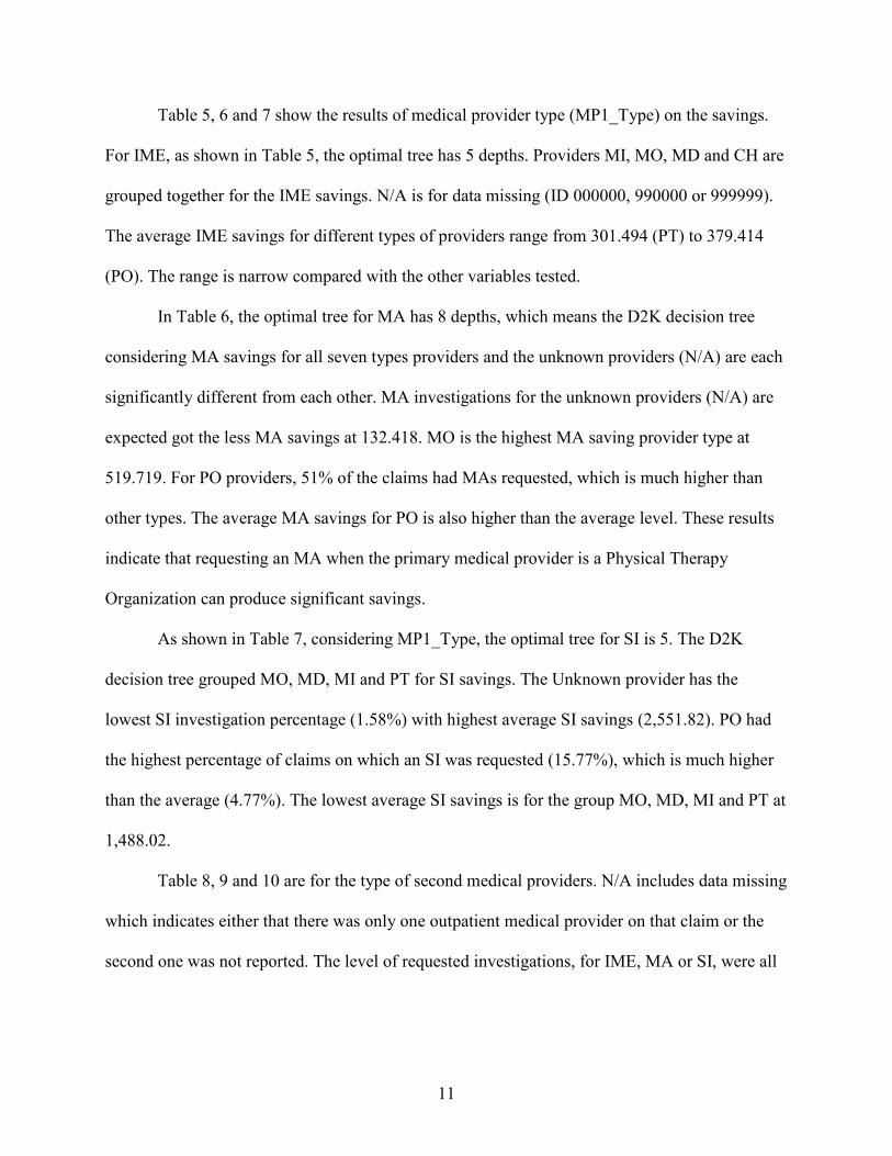
Table 5, 6 and 7 show the results of medical provider type (MP1_Type) on the savings.

For IME, as shown in Table 5, the optimal tree has 5 depths. Providers MI, MO, MD and CH are

grouped together for the IME savings. N/A is for data missing (ID 000000, 990000 or 999999).

The average IME savings for different types of providers range from 301.494 (PT) to 379.414

(PO). The range is narrow compared with the other variables tested.

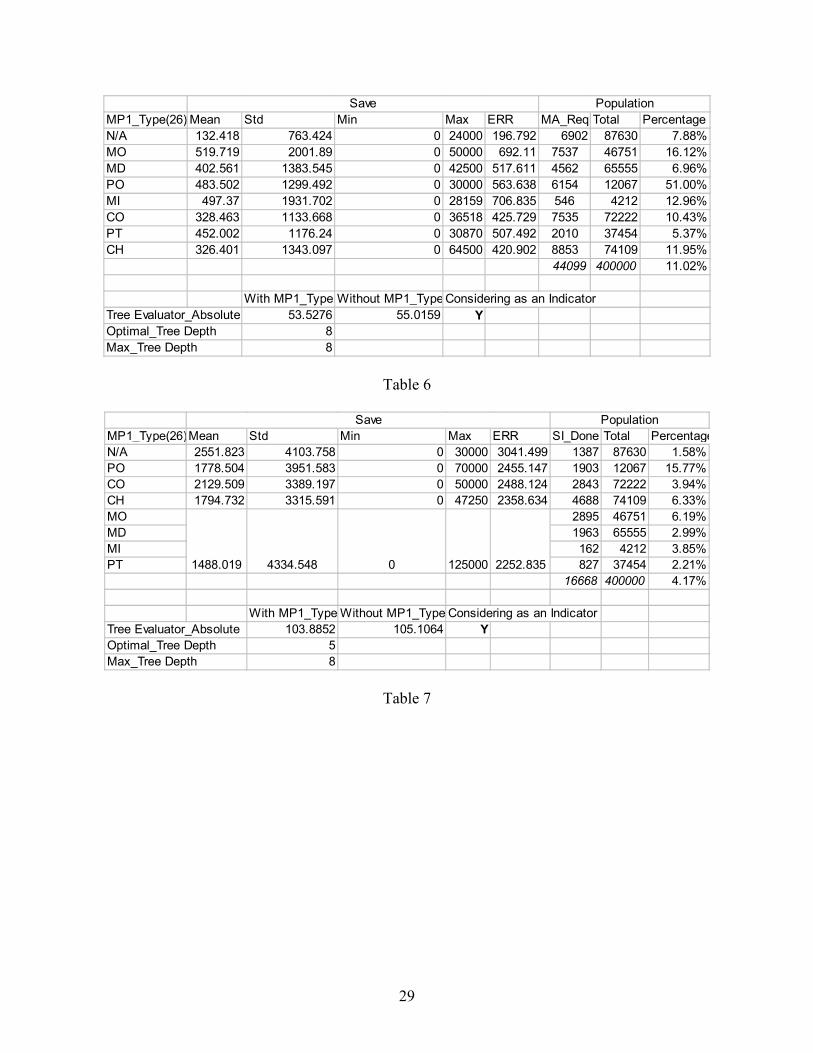
In Table 6, the optimal tree for MA has 8 depths, which means the D2K decision tree

considering MA savings for all seven types providers and the unknown providers (N/A) are each

significantly different from each other. MA investigations for the unknown providers (N/A) are

expected got the less MA savings at 132.418. MO is the highest MA saving provider type at

519.719. For PO providers, 51% of the claims had MAs requested, which is much higher than

other types. The average MA savings for PO is also higher than the average level. These results

indicate that requesting an MA when the primary medical provider is a Physical Therapy

Organization can produce significant savings.

As shown in Table 7, considering MP1_Type, the optimal tree for SI is 5. The D2K

decision tree grouped MO, MD, MI and PT for SI savings. The Unknown provider has the

lowest SI investigation percentage (1.58%) with highest average SI savings (2,551.82). PO had

the highest percentage of claims on which an SI was requested (15.77%), which is much higher

than the average (4.77%). The lowest average SI savings is for the group MO, MD, MI and PT at

1,488.02.

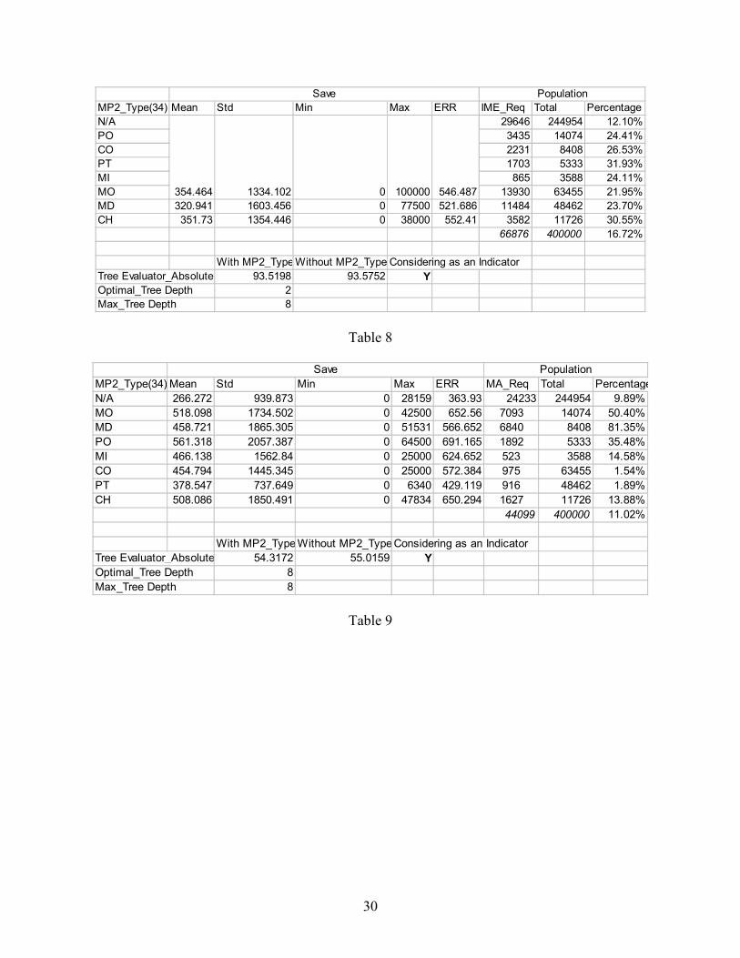
Table 8, 9 and 10 are for the type of second medical providers. N/A includes data missing

which indicates either that there was only one outpatient medical provider on that claim or the

second one was not reported. The level of requested investigations, for IME, MA or SI, were all

12

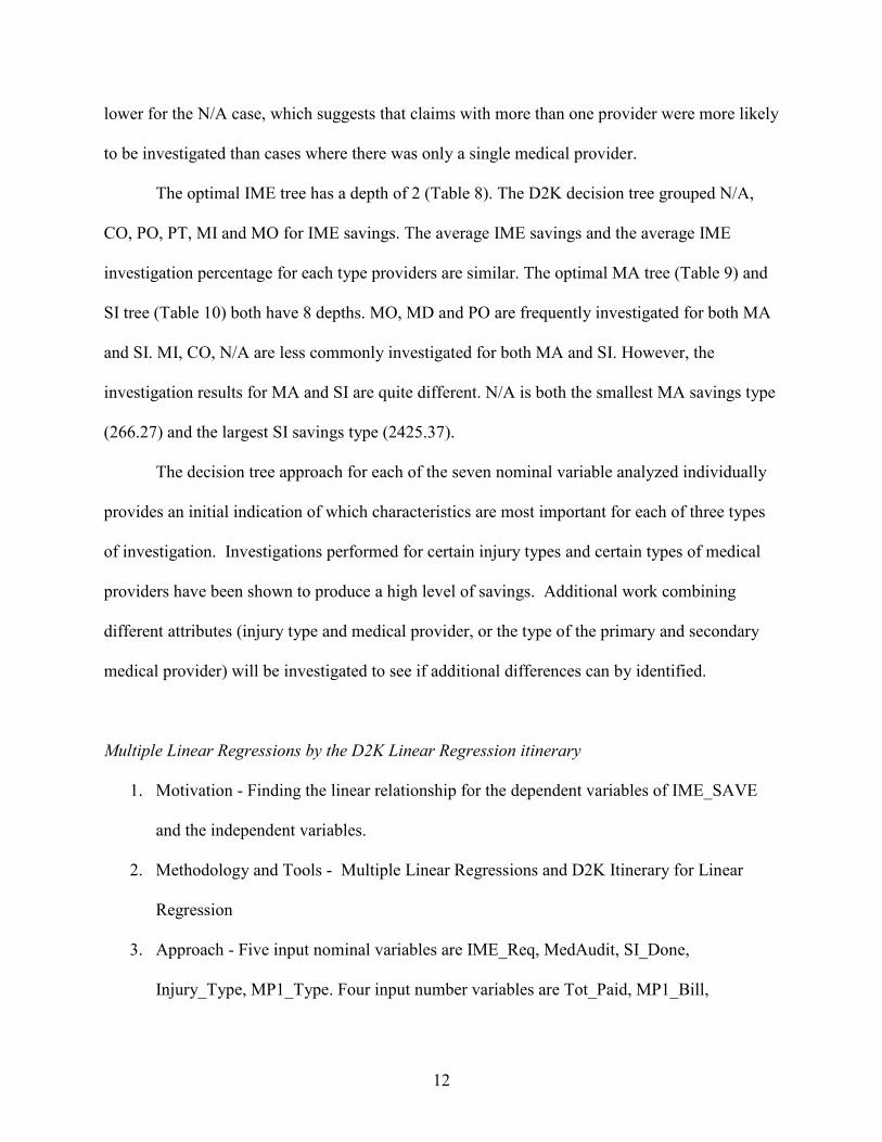
lower for the N/A case, which suggests that claims with more than one provider were more likely

to be investigated than cases where there was only a single medical provider.

The optimal IME tree has a depth of 2 (Table 8). The D2K decision tree grouped N/A,

CO, PO, PT, MI and MO for IME savings. The average IME savings and the average IME

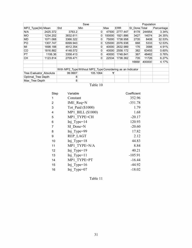
investigation percentage for each type providers are similar. The optimal MA tree (Table 9) and

SI tree (Table 10) both have 8 depths. MO, MD and PO are frequently investigated for both MA

and SI. MI, CO, N/A are less commonly investigated for both MA and SI. However, the

investigation results for MA and SI are quite different. N/A is both the smallest MA savings type

(266.27) and the largest SI savings type (2425.37).

The decision tree approach for each of the seven nominal variable analyzed individually

provides an initial indication of which characteristics are most important for each of three types

of investigation. Investigations performed for certain injury types and certain types of medical

providers have been shown to produce a high level of savings. Additional work combining

different attributes (injury type and medical provider, or the type of the primary and secondary

medical provider) will be investigated to see if additional differences can by identified.

Multiple Linear Regressions by the D2K Linear Regression itinerary

1. Motivation - Finding the linear relationship for the dependent variables of IME_SAVE

and the independent variables.

2. Methodology and Tools - Multiple Linear Regressions and D2K Itinerary for Linear

Regression

3. Approach - Five input nominal variables are IME_Req, MedAudit, SI_Done,

Injury_Type, MP1_Type. Four input number variables are Tot_Paid, MP1_Bill,

13

TREATLAG, REP_LAGT. The dependent variable is IME_Saved. The five input

nominal variables are treated as 38 nominal input features according to the 38 possible

values. Therefore, there are 42 input variables.

The dataset was separated into training dataset (400,000) and testing dataset (91,591). The

forward stepwise method was practiced to test the linear models. The D2K Linear Regression

program started the linear regression from one variable case. All possible single variable

regressions were completed by the training dataset. Then the testing dataset selected one of the

best regression formulas with the most significant variable, which minimized the external error.

Based on the single regression, D2K Linear Regression program added one additional variable to

the selected single variable regression by trying all variables one by one. The testing process was

the following step. All two-variable regressions were tested by the testing dataset. The optimal

regression minimized the external error (including the external error of single variable

regression). This training and testing process continued until the optimal regression that

minimized the external error was determined.

The regression stopped at 16th step due to the computer resource. The optimal linear

model is the 15-variable regression model determined at step 16. Model variables with the

coefficients in the determined order are provided in the table 11. The constant term is 352.96.

The coefficient for no IME requested was -351.78, meaning that the total savings would be

approximately zero (352.96-351.78) if no IME were requested. The number variables of Total

Paid, MP1_Bill and REP Lag are positively related to the IME saved. The nominal (dummy)

variables of IME Request, SI Done, Injury Type 14, 18, 19, 99 and MP1 Type=N/A increase the

IME saved. The nominal variables of MP1 Type=CH, PT and Injury Type 7, 11, 16 decrease the

IME saved.

14

Additional Analyses

A series of additional analyses were performed using SAS to gain a better understanding

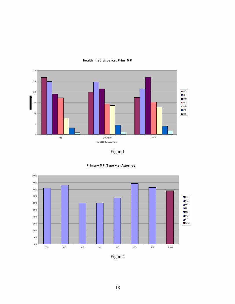
of the dataset. The most significant results are illustrated in the following figures. Figure 1

illustrates the relationship between the types of Primary Medical Provider and Health insurance.

The claims are grouped by the health insurance status- yes, no or unknown. For each claims

group, the percentages of Primary Medical Provider’s Type were shown at y-axis. In the No

health insurance group, most claimants chose CO type provider. In the Yes group, most

claimants prefer MO type provider. The type of medical provider is strongly influenced by the

presence of health insurance.

Figure 2 illustrates the attorney representation frequency according to the different types

of providers. According to the bars, the PO, CO and CH providers have the highest attorney

representation, over 80%. MD, MI and MO have a lower attorney representation, around 60%.

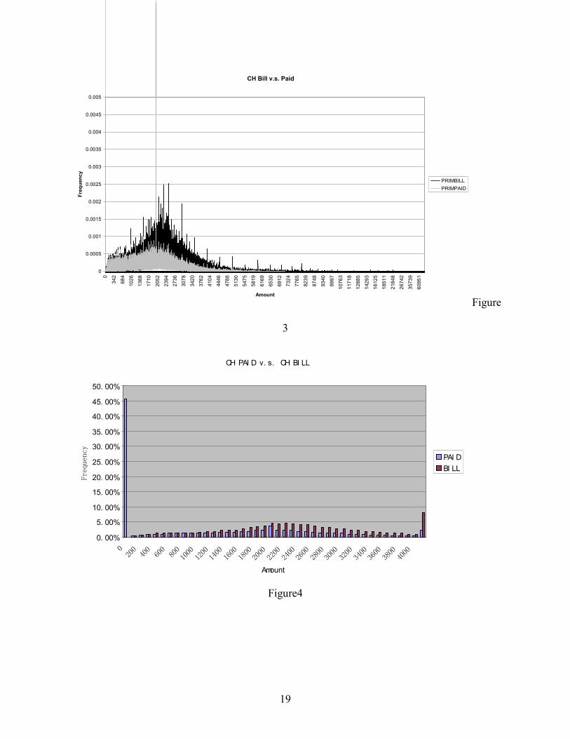
Figures 3 and 4 illustrate the distributions of Amount Billed and Amount Paid for CH

providers in PIP claims. In Figure 3, the x-axis is the actual value of the amount billed or paid.

In Figure 4, the amounts are grouped into ranges. The blue area is for the paid; the pink area is

for the bill. The distribution of the amount of the bill has the general shape of a Normal

distribution. The paid distribution has two mass points of 0 (45.65%) and 2000 (1.47%),

indicating that 45.65% of the bills had no medical payments (BI claims do not cover medical

bills), and 1.47% of the bills are covered with a $2000 payment, the tort threshold in

Massachusetts and the primary coverage for PIP in the presence of private health insurance.

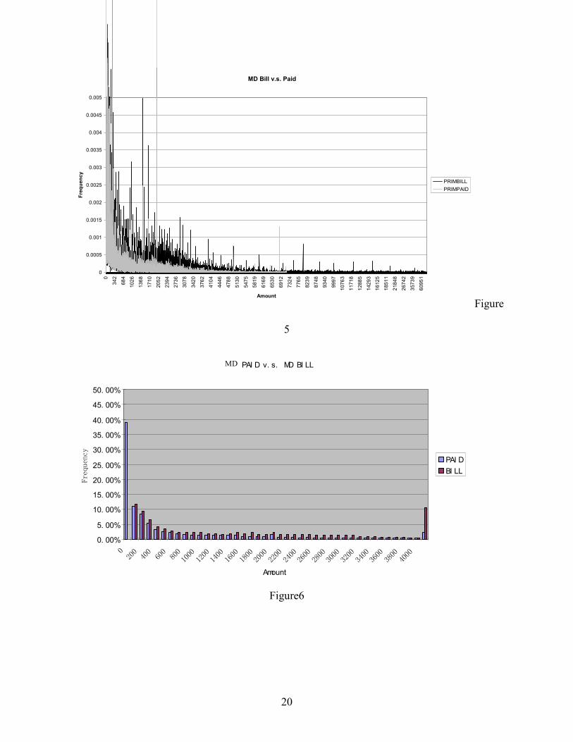
Figure 5 and 6 illustrate the distributions of Amount Billed and Amount Paid for MD

providers. The blue area is for the paid; the pink area is for the bill. Comparing with CH

providers, the distributions for both Bill and Paid are more discrete. The two mass points for paid

15

distribution are 0 (38.86%) and 2000 (0.98%). These percentages are smaller than for the CH

providers. Unlike the distribution for CH providers, these distributions appear to be shaped more

like a lognormal distribution, with more values concentrated around 0 compared with CH

providers.

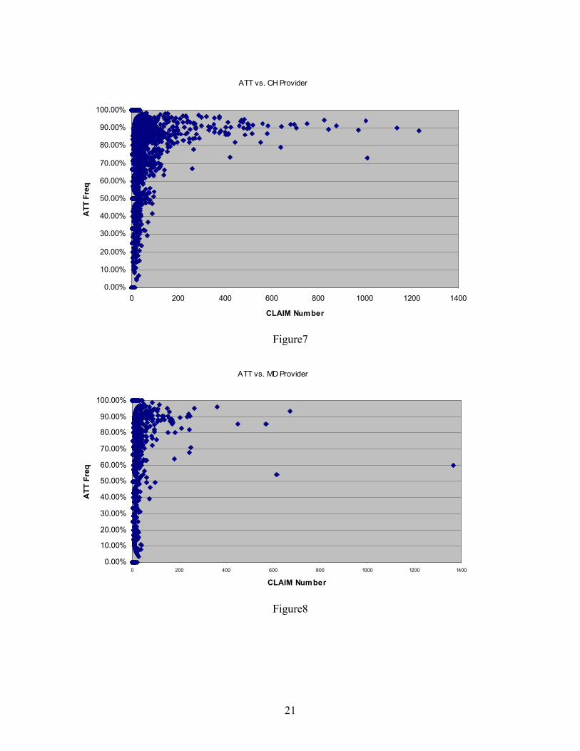
Figures 7 and 8 illustrate the distributions of Attorney representation frequency according

to the number of claims a medical provider was involved with for CH (Figure 7) and MD (Figure

8) providers. Each point in the figure represents a provider. The x-axis coordination is the

number of claims in the dataset for this provider; the y-axis coordination is the attorney

representation frequency for this provider. When the claim numbers increase, the attorney

frequencies for the CH appear to increase, and then level out around 90%; for MDs, the attorney

frequency appears to decrease for the providers with the greatest number of claims, at least for

the outliers.

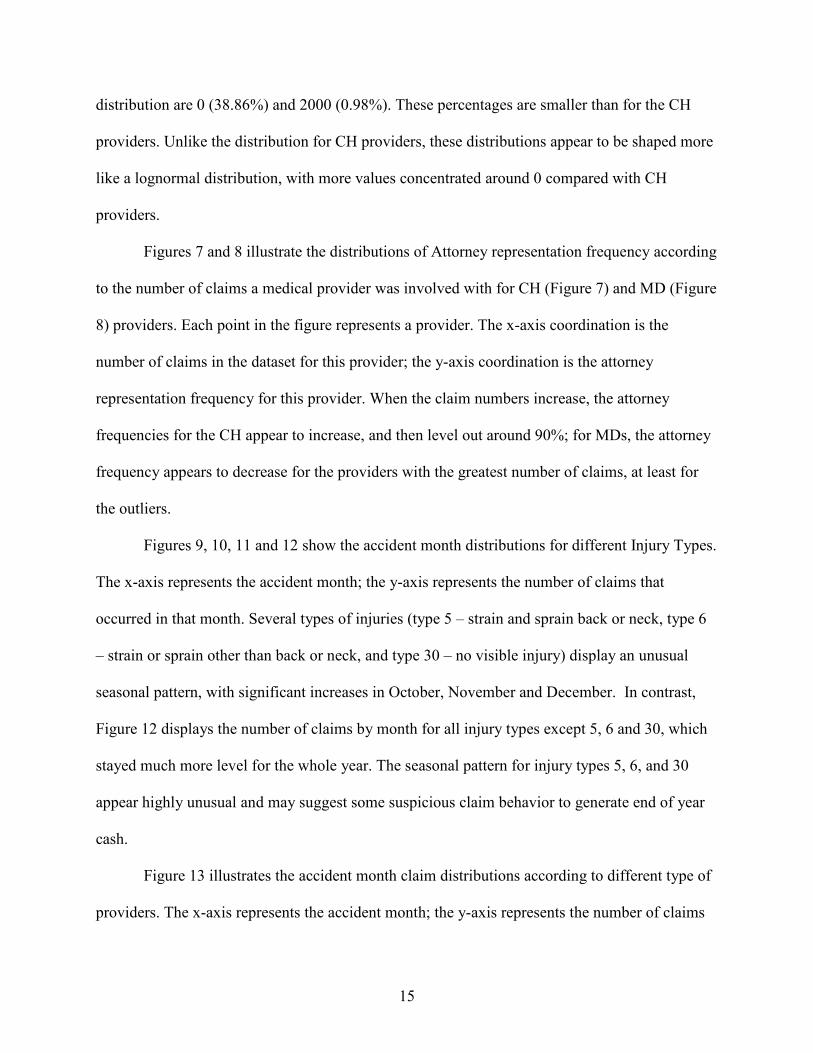
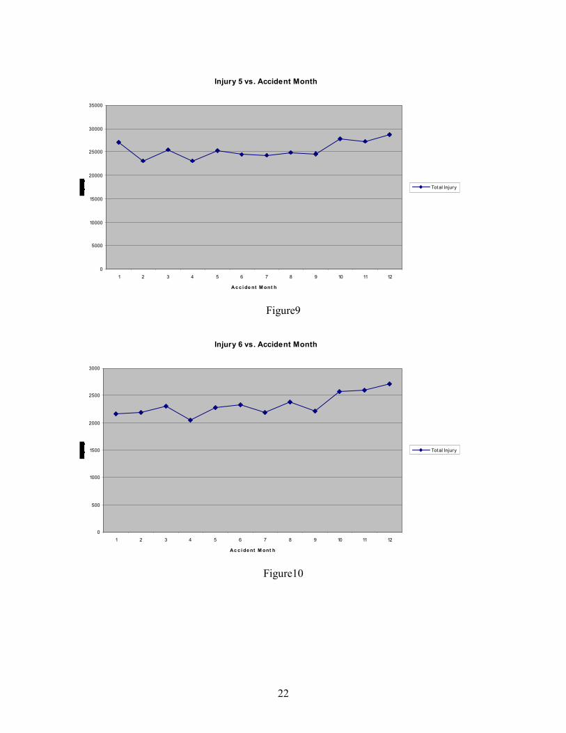
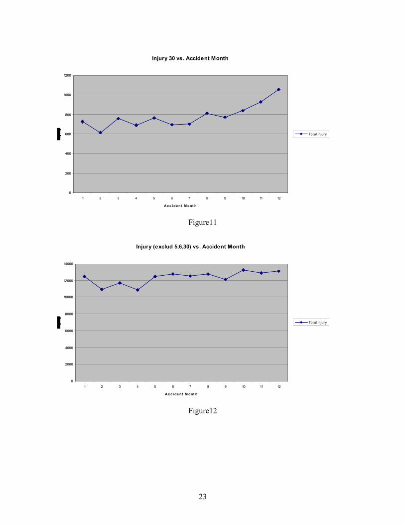
Figures 9, 10, 11 and 12 show the accident month distributions for different Injury Types.

The x-axis represents the accident month; the y-axis represents the number of claims that

occurred in that month. Several types of injuries (type 5 – strain and sprain back or neck, type 6

– strain or sprain other than back or neck, and type 30 – no visible injury) display an unusual

seasonal pattern, with significant increases in October, November and December. In contrast,

Figure 12 displays the number of claims by month for all injury types except 5, 6 and 30, which

stayed much more level for the whole year. The seasonal pattern for injury types 5, 6, and 30

appear highly unusual and may suggest some suspicious claim behavior to generate end of year

cash.

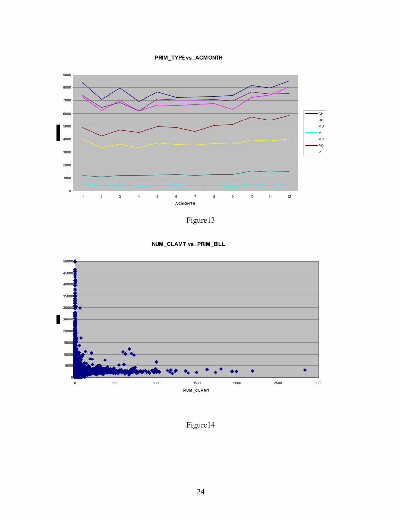
Figure 13 illustrates the accident month claim distributions according to different type of

providers. The x-axis represents the accident month; the y-axis represents the number of claims

16

that occurred in that month. The distributions for different provider types are represented by

different color lines. The CH, CO and PO lines increase significantly at the end of the year. The

lines for MD, PT and MI stayed at a relatively steady level for the whole year.

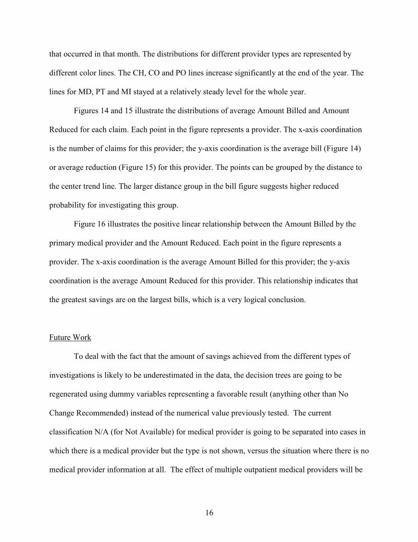
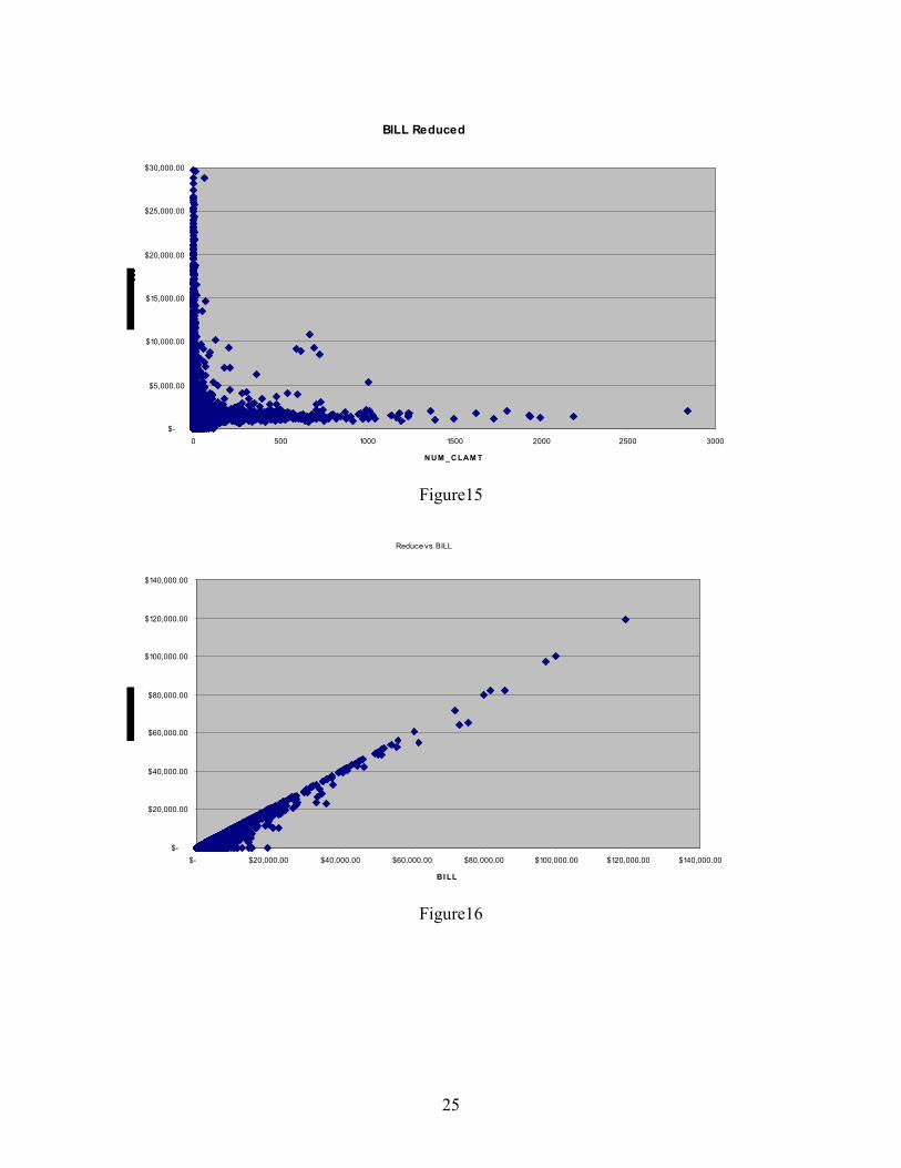
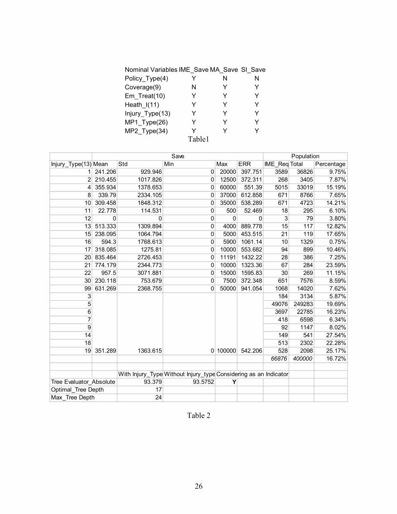
Figures 14 and 15 illustrate the distributions of average Amount Billed and Amount

Reduced for each claim. Each point in the figure represents a provider. The x-axis coordination

is the number of claims for this provider; the y-axis coordination is the average bill (Figure 14)

or average reduction (Figure 15) for this provider. The points can be grouped by the distance to

the center trend line. The larger distance group in the bill figure suggests higher reduced

probability for investigating this group.

Figure 16 illustrates the positive linear relationship between the Amount Billed by the

primary medical provider and the Amount Reduced. Each point in the figure represents a

provider. The x-axis coordination is the average Amount Billed for this provider; the y-axis

coordination is the average Amount Reduced for this provider. This relationship indicates that

the greatest savings are on the largest bills, which is a very logical conclusion.

Future Work

To deal with the fact that the amount of savings achieved from the different types of

investigations is likely to be underestimated in the data, the decision trees are going to be

regenerated using dummy variables representing a favorable result (anything other than No

Change Recommended) instead of the numerical value previously tested. The current

classification N/A (for Not Available) for medical provider is going to be separated into cases in

which there is a medical provider but the type is not shown, versus the situation where there is no

medical provider information at all. The effect of multiple outpatient medical providers will be

17

investigated to determine if particular combinations of providers (such as two physical therapists,

or a chiropractor and a physical therapist) indicate greater potential savings from investigations.

In order to get more sensitive indicators, injury types will be combined (strains and sprains,

minor injuries, serious injuries, major injuries or fatalities) for machine learning techniques.

The seasonality effect for certain types of injures (as illustrated in Figures 9-12) will be

used to identify those injury types that may be linked to fraudulent claiming behavior, and

incorporated into further D2K decision trees. Additional work will incorporate information

regarding attorney representation, accident location and the timing of seeking medical treatment

to generate more significant predictive models.

Additional multiple regressions will be run for MA and SI savings, and greater computer

resources will be used to allow for more steps and more variables in the process. These runs will

identify the most important variables, or combination of variables, that affect the savings from

investigations.

To date the programs have been run on the entire dataset. Future analyses will be run

separately by coverage to isolate differences between PIP and BI claims.

Conclusion

Predictive modeling provides a set of valuable tools for insurance companies for a variety

of purposes, from pricing to underwriting to claims handling. This work represents a start on this

process for determining the optimal strategy for investigating claim to reduce medical costs, but

there is a long way to go to get fully coherent and meaningful results. Comments and

suggestions on this work would be greatly appreciated.

18

Figure1

Figure2

Health_Insurance v.s. Prim_MP

0

5

10

15

20

25

30

No Unknown Yes

Hea l t h I nsur ance

CO

CH

MO

PO

MD

PT

MI

Primary MP_Type v.s. Attorney

0%

10%

20%

30%

40%

50%

60%

70%

80%

90%

100%

CH CO MD MI MO PO PT Tot al

CH

CO

MD

MI

MO

PO

PT

Tot al

19

CH Bill v.s. Paid

0

0.0005

0.001

0.0015

0.002

0.0025

0.003

0.0035

0.004

0.0045

0.005

0

34

2

68

4

10

26

13

68

17

10

20

52

23

94

27

36

30

78

34

20

37

62

41

04

44

46

47

88

51

30

54

75

58

19

61

69

65

30

69

12

73

24

77

65

82

39

87

48

93

40

99

97

10

76

3

11

71

8

12

88

5

14

29

3

16

12

5

18

51

1

21

84

8

26

74

2

35

73

9

60

95

1

Amount

Frequency

PRIMBILL

PRIMPAID

Figure

3

Figure4

CH PAI D v. s. CH BI LL

0. 00%

5. 00%

10. 00%

15. 00%

20. 00%

25. 00%

30. 00%

35. 00%

40. 00%

45. 00%

50. 00%

0200

400

600

8001000

1200

1400

1600

1800

2000

2200

2400

2600

2800

3000

3200

3400

3600

3800

4000

Amount

Frequency

PAI D

BI LL

20

MD Bill v.s. Paid

0

0.0005

0.001

0.0015

0.002

0.0025

0.003

0.0035

0.004

0.0045

0.005

0

34

2

68

4

10

26

13

68

17

10

20

52

23

94

27

36

30

78

34

20

37

62

41

04

44

46

47

88

51

30

54

75

58

19

61

69

65

30

69

12

73

24

77

65

82

39

87

48

93

40

99

97

10

76

3

11

71

8

12

88

5

14

29

3

16

12

5

18

51

1

21

84

8

26

74

2

35

73

9

60

95

1

Amount

Frequency

PRIMBILL

PRIMPAID

Figure

5

Figure6

MD PAI D v. s. MD BI LL

0. 00%

5. 00%

10. 00%

15. 00%

20. 00%

25. 00%

30. 00%

35. 00%

40. 00%

45. 00%

50. 00%

0200

400

600

8001000

1200

1400

1600

1800

2000

2200

2400

2600

2800

3000

3200

3400

3600

3800

4000

Amount

Frequency

PAI D

BI LL

21

Figure7

Figure8

ATT vs. CH Provider

0.00%

10.00%

20.00%

30.00%

40.00%

50.00%

60.00%

70.00%

80.00%

90.00%

100.00%

0 200 400 600 800 1000 1200 1400

CLAIM Number

ATT Freq

ATT vs. MD Provider

0.00%

10.00%

20.00%

30.00%

40.00%

50.00%

60.00%

70.00%

80.00%

90.00%

100.00%

0 200 400 600 800 1000 1200 1400

CLAIM Number

ATT Freq

22

Figure9

Figure10

Injury 5 vs. Accident Month

0

5000

10000

15000

20000

25000

30000

35000

1 2 3 4 5 6 7 8 9 10 11 12

Acc ide nt Mont h

Tot al Injury


0

500

1000

1500

2000

2500

3000

1 2 3 4 5 6 7 8 9 10 11 12

Acc ident Mont h

Tot al Injury

23

Figure11

Figure12


0

200

400

600

800

1000

1200

1 2 3 4 5 6 7 8 9 10 11 12

Acc ident Mont h

Tot al Injury

Injury (exclud 5,6,30) vs. Accident Month

0

2000

4000

6000

8000

10000

12000

14000

1 2 3 4 5 6 7 8 9 10 11 12

Acc ident Mont h

Tot al Injury

24

Figure13

Figure14

PRIM_TYPE vs. ACMONTH

0

1000

2000

3000

4000

5000

6000

7000

8000

9000

1 2 3 4 5 6 7 8 9 10 11 12

ACMONTH

CH

CO

MD

MI

MO

PO

PT

NUM_CLAMT vs. PRIM_BILL

0

5000

10000

15000

20000

25000

30000

35000

40000

45000

50000

0 500 1000 1500 2000 2500 3000

NUM_CLAMT

25

Figure15

Figure16

BILL Reduced

$-

$5,000.00

$10,000.00

$15,000.00

$20,000.00

$25,000.00

$30,000.00

0 500 1000 1500 2000 2500 3000

NUM_CLAMT

Reduce vs. BILL

$-

$20,000.00

$40,000.00

$60,000.00

$80,000.00

$100,000.00

$120,000.00

$140,000.00

$- $20,000.00 $40,000.00 $60,000.00 $80,000.00 $100,000.00 $120,000.00 $140,000.00

BILL

26

Nominal Variables IME_Save MA_Save SI_Save

Policy_Type(4) Y N N

Coverage(9) N Y Y

Em_Treat(10) Y Y Y

Heath_I(11) Y Y Y

Injury_Type(13) Y Y Y

MP1_Type(26) Y Y Y

MP2_Type(34) Y Y Y

Table1

Injury_Type(13) Mean Std Min Max ERR IME_Req Total Percentage

1 241.206 929.946 0 20000 397.751 3589 36826 9.75%

2 210.455 1017.826 0 12500 372.311 268 3405 7.87%

4 355.934 1378.653 0 60000 551.39 5015 33019 15.19%

8 339.79 2334.105 0 37000 612.858 671 8766 7.65%

10 309.458 1848.312 0 35000 538.289 671 4723 14.21%

11 22.778 114.531 0 500 52.469 18 295 6.10%

12 0 0 0 0 0 3 79 3.80%

13 513.333 1309.894 0 4000 889.778 15 117 12.82%

15 238.095 1064.794 0 5000 453.515 21 119 17.65%

16 594.3 1768.613 0 5900 1061.14 10 1329 0.75%

17 318.085 1275.81 0 10000 553.682 94 899 10.46%

20 835.464 2726.453 0 11191 1432.22 28 386 7.25%

21 774.179 2344.773 0 10000 1323.36 67 284 23.59%

22 957.5 3071.881 0 15000 1595.83 30 269 11.15%

30 230.118 753.679 0 7500 372.348 651 7576 8.59%

99 631.269 2368.755 0 50000 941.054 1068 14020 7.62%

3 184 3134 5.87%

5 49076 249283 19.69%

6 3697 22785 16.23%

7 418 6598 6.34%

9 92 1147 8.02%

14 149 541 27.54%

18 513 2302 22.28%

19 528 2098 25.17%

66876 400000 16.72%

With Injury_Type Without Injury_type Considering as an Indicator

Tree Evaluator_Absolute 93.379 93.5752 Y

Optimal_Tree Depth 17

Max_Tree Depth 24

Save Population

351.289 1363.615 0 100000 542.206

Table 2

27

Injury_Type(13) Mean Std Min Max ERR MA_Req Total Percentage

1 198.748 906.586 0 30870 272.908 3670 36826 9.97%

2 338 3405 9.93%

3 126 3134 4.02%

4 5309 33019 16.08%

5 27931 249283 11.20%

6 2699 22785 11.85%

7 650 6598 9.85%

8 877 8766 10.00%

9 114 1147 9.94%

10 541 4723 11.45%

11 23 295 7.80%

12 6 79 7.59%

13 15 117 12.82%

14 75 541 13.86%

15 14 119 11.76%

16 34 1329 2.56%

17 91 899 10.12%

18 275 2302 11.95%

19 241 2098 11.49%

20 36 386 9.33%

21 40 284 14.08%

22 30 269 11.15%

30 381 7576 5.03%

99 583 14020 4.16%

44099 400000 11.02%




Max_Tree Depth 24

Save Population

382.357 1418.852 0 64500 499.849

Table 3

28

Injury_Type(13) Mean Std Min Max ERR SI_Done Total Percentage

1 802.954 2544.6 0 29000 1355.145 1061 36826 2.88%

3 2077.654 4089.497 0 20000 2821.898 136 3134 4.34%

4 923.126 2647.884 0 25000 1478.106 1170 33019 3.54%

5 2054.337 3714.105 0 100000 2557.582 11298 249283 4.53%

10 669.551 2588.603 0 20000 1183.831 196 4723 4.15%

12 0 0 0 0 0 4 79 5.06%

13 5600 7838.367 0 20000 6720 5 117 4.27%

15 12857.14 25892.241 0 75000 18367.35 7 119 5.88%

16 666.667 3265.986 0 20000 1274.074 45 1329 3.39%

18 996.253 3367.884 0 36500 1680.881 221 2302 9.60%

20 0 0 0 0 0 11 386 2.85%

99 1921.895 3593.821 0 20000 2603.499 306 14020 2.18%

2 141 3405 4.14%

6 797 22785 3.50%

7 280 6598 4.24%

8 353 8766 4.03%

9 45 1147 3.92%

11 7 295 2.37%

14 30 541 5.55%

17 34 899 3.78%

19 243 2098 11.58%

21 20 284 7.04%

22 13 269 4.83%

30 245 7576 3.23%

16668 400000 4.17%




Max_Tree Depth 24

Save Population

1621.494 5131.193 0 125000 2529.773

Table 4

MP1_Type(26) Mean Std Min Max ERR IME_Req Total Percentage

N/A 358.812 1127.875 0 17000 570.734 2073 87630 2.37%

PO 379.414 1299.146 0 38000 589.951 9349 46751 20.00%CO 350.128 987.217 0 18000 515.598 15366 65555 23.44%

PT 301.494 988.623 0 17500 483.896 3009 12067 24.94%

MI 764 4212 18.14%

MO 11167 72222 15.46%MD 6351 37454 16.96%

CH 18797 74109 25.36%

66876 400000 16.72%

With MP1_Type Without MP1_Type Considering as an Indicator


Optimal_Tree Depth 5Max_Tree Depth 8

Save Population

343.643 1537.258 0 100000 544.51

Table 5

29

MP1_Type(26) Mean Std Min Max ERR MA_Req Total Percentage

N/A 132.418 763.424 0 24000 196.792 6902 87630 7.88%

MO 519.719 2001.89 0 50000 692.11 7537 46751 16.12%

MD 402.561 1383.545 0 42500 517.611 4562 65555 6.96%

PO 483.502 1299.492 0 30000 563.638 6154 12067 51.00%

MI 497.37 1931.702 0 28159 706.835 546 4212 12.96%

CO 328.463 1133.668 0 36518 425.729 7535 72222 10.43%

PT 452.002 1176.24 0 30870 507.492 2010 37454 5.37%

CH 326.401 1343.097 0 64500 420.902 8853 74109 11.95%

44099 400000 11.02%




Max_Tree Depth 8

Save Population

Table 6

MP1_Type(26) Mean Std Min Max ERR SI_Done Total Percentage

N/A 2551.823 4103.758 0 30000 3041.499 1387 87630 1.58%

PO 1778.504 3951.583 0 70000 2455.147 1903 12067 15.77%

CO 2129.509 3389.197 0 50000 2488.124 2843 72222 3.94%

CH 1794.732 3315.591 0 47250 2358.634 4688 74109 6.33%

MO 2895 46751 6.19%

MD 1963 65555 2.99%

MI 162 4212 3.85%

PT 827 37454 2.21%

16668 400000 4.17%




Max_Tree Depth 8

Save Population

1488.019 4334.548 0 125000 2252.835

Table 7

30

MP2_Type(34) Mean Std Min Max ERR IME_Req Total Percentage

N/A 29646 244954 12.10%

PO 3435 14074 24.41%

CO 2231 8408 26.53%

PT 1703 5333 31.93%

MI 865 3588 24.11%

MO 13930 63455 21.95%

MD 320.941 1603.456 0 77500 521.686 11484 48462 23.70%

CH 351.73 1354.446 0 38000 552.41 3582 11726 30.55%

66876 400000 16.72%




Max_Tree Depth 8

Save Population

354.464 1334.102 0 100000 546.487

Table 8

MP2_Type(34) Mean Std Min Max ERR MA_Req Total Percentage

N/A 266.272 939.873 0 28159 363.93 24233 244954 9.89%

MO 518.098 1734.502 0 42500 652.56 7093 14074 50.40%

MD 458.721 1865.305 0 51531 566.652 6840 8408 81.35%

PO 561.318 2057.387 0 64500 691.165 1892 5333 35.48%

MI 466.138 1562.84 0 25000 624.652 523 3588 14.58%

CO 454.794 1445.345 0 25000 572.384 975 63455 1.54%

PT 378.547 737.649 0 6340 429.119 916 48462 1.89%

CH 508.086 1850.491 0 47834 650.294 1627 11726 13.88%

44099 400000 11.02%




Max_Tree Depth 8

Save Population

Table 9

31

MP2_Type(34) Mean Std Min Max ERR SI_Done Total Percentage

N/A 2425.372 3763.2 0 47500 2777.447 8178 244954 3.34%

MO 1234.202 3832.611 0 100000 1921.886 3427 14074 24.35%

MD 1071.068 3366.322 0 75000 1738.958 2735 8408 32.53%

PO 1307.747 6099.943 0 125000 2076.938 668 5333 12.53%

MI 1698.188 4912.354 0 40000 2632.989 176 3588 4.91%

CO 1816.882 4148.572 0 40000 2558.172 382 63455 0.60%

PT 1106.36 3358.413 0 40000 1748.841 367 48462 0.76%

CH 1123.814 2709.471 0 22534 1738.362 735 11726 6.27%

16668 400000 4.17%




Max_Tree Depth 8

Save Population

Table 10

Step Variable Coefficient

1 Constant 352.96

2 IME_Req=N -351.78

3 Tot_Paid ($1000) 1.79

4 MP1_BILL ($1000) 1.68

5 MP1_TYPE=CH -20.17

6 Inj_Type=14 120.93

7 SI_Done=N -20.60

8 Inj_Type=99 17.82

9 REP_LAGT 2.12

10 Inj_Type=18 44.83

11 MP1_TYPE=N/A 8.84

12 Inj_Type=19 40.21

13 Inj_Type=11 -105.91

14 MP1_TYPE=PT -16.44

15 Inj_Type=16 -44.92

16 Inj_Type=07 -18.02

Table 11

32

References

Brockett, Patrick L., Derrig, Richard A., Golden, Linda L., Levine, Arnold, and Alpert, Mark, 2002, Fraud Classification Using Principal Component Analysis of RIDITS, Journal of Risk and Insurance, 69:3 341-372. Brockett, Patrick L., Xia, Xiaohua, and Derrig, Richard A, 1998, Using Kohonen’s Self-Organizing Feature Map to Uncover Automobile Bodily Injury Claims Fraud, Journal of Risk and Insurance, 65:2 245-274. Derrig, Richard A., 2003, Overview of Detail Claim Database of Massachusetts, Automobile Insurers Bureau Memorandum, July 9, 2003. Derrig, Richard A. and Weisberg, Herbert I., 2003, Auto Bodily Injury Claim Settlement in Massachusetts: Final Results of Claim Screen Experiment, Automobile Insurers Bureau of Massachusetts Working Paper. Hsu, William H., Welge, Michael, Redman, Tom, and Clutter, David, 2002, High Performance Commercial Data Mining: A Multistrategy Machine Learning Application, Data Mining and Knowledge Discovery, 6 361-391. Tennyson, Sharon and Salsas-Forn, Pau, 2002, Claims Auditing in Automobile Insurance: Fraud Detection and Deterrence Objectives, Journal of Risk and Insurance, 69:3 289-308. Viaene, Stijn, Derrig, Richard A., Baesens, Bart and Dedene, Guido, 2002, A Comparison of State-of-the-Art Classification Techniques for Expert Automobile Insurance Claim Fraud Detection, Journal of Risk and Insurance, 69:3 373-421.

Documents

Predictive Modeling in Automobile Insurance 7-1-05 Modeling in Automobile... · 1 Predictive Modeling in Automobile Insurance: A Preliminary Analysis Stephen P. D’Arcy Abstract