Embed Size (px)
Citation preview

Sandesh Poudel
Predictive Analytics of Digital Marketing and Sales Pipeline
Metropolia University of Applied Sciences
Bachelor of Engineering
Information Technology
Bachelor’s Thesis
20 November 2019
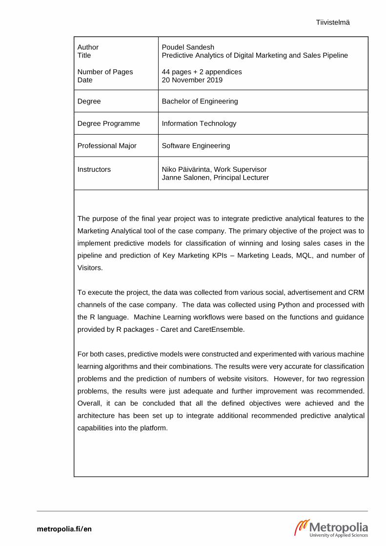
Tiivistelmä
Author Title Number of Pages Date
Poudel Sandesh Predictive Analytics of Digital Marketing and Sales Pipeline 44 pages + 2 appendices 20 November 2019
Degree Bachelor of Engineering
Degree Programme Information Technology
Professional Major Software Engineering
Instructors
Niko Päivärinta, Work Supervisor Janne Salonen, Principal Lecturer
The purpose of the final year project was to integrate predictive analytical features to the
Marketing Analytical tool of the case company. The primary objective of the project was to
implement predictive models for classification of winning and losing sales cases in the
pipeline and prediction of Key Marketing KPIs – Marketing Leads, MQL, and number of
Visitors.
To execute the project, the data was collected from various social, advertisement and CRM
channels of the case company. The data was collected using Python and processed with
the R language. Machine Learning workflows were based on the functions and guidance
provided by R packages - Caret and CaretEnsemble.
For both cases, predictive models were constructed and experimented with various machine
learning algorithms and their combinations. The results were very accurate for classification
problems and the prediction of numbers of website visitors. However, for two regression
problems, the results were just adequate and further improvement was recommended.
Overall, it can be concluded that all the defined objectives were achieved and the
architecture has been set up to integrate additional recommended predictive analytical
capabilities into the platform.

Tiivistelmä
Keywords Predictive Analytics, Machine Learning, Digital Marketing, Sales Pipeline, Artificial Intelligence, Caret Package
Contents
List of Abbreviations
1 Introduction 1
2 Theoretical Background 2
2.1 Digital Marketing 2
2.1.1 CRM and Sales Pipeline 3
2.1.2 Marketing Funnel 3
2.1.3 Marketing Key Perfomance Indicators 5
2.2 Predictive Analytics 5
2.2.1 Artificial Intelligence (AI) and Machine Learning 6
2.2.2 Learning Techniques 7
2.2.3 Supervised Learning Algorithms 9
3 Current State Analysis 14
3.1 Inline Insight 15
3.2 Advanced Analytics and Prediction 15
3.3 Limitation and issues 16
3.4 Objectives 16
4 Methods and Materials 17
4.1 Tools and Technologies 17
4.1.1 Python 18
4.1.2 R 18
4.2 Data 19
4.3 Implementation 20
4.3.1 Data Preparation 20
4.3.2 Descriptive Analytics 20
4.3.3 Data Splitting and pre-processing 21
4.3.4 Feature Selection 26
4.3.5 Training and Turning Models 27
4.3.6 Ensemble Models 28
4.4 Model Evaluation 29

4.4.1 Regression problems 29
4.4.2 Classification problem 30
5 Result and Discussions 31
5.1 Benchmark Result 31
5.1.1 Deal classification case 32
5.1.2 KPIs prediction case 34
5.2 Further improvement 37
6 Conclusion and Summary 38
References 40
Appendices
Appendix 1. Results for Deal classification case
Appendix 2. Results for Lead prediction cases
List of Abbreviations
KPI Key Performance Indicator
SMS Short Message Service
MMS Multimedia Messaging Service
ROI Return on Investments
TOFU Top Of The Funnel
MOFU Middle Of The Funnel
BOFU Bottom Of The Funnel
KW Kilowatt
AI Artificial Intelligence
ATM Automated Teller Machine
SOM Self Organizing Map
SQL Structured Query Language
ETL Extract Transform Load
BI Business Intelligence
SaaS Software as a Service
CSV Comma Separated Values
API Application Programming Interface
MQL Marketing Qualified Leads
CRM Customer Relationship Management

KNN K Nearest Neighbors
ROC Receiver Operating Characteristics
RMSE Root Mean Square Error
MAPE Mean Absolute Percentage Error
AUC Area Under the Curve
ETL Extract Transform Load
1 (44)
1 Introduction
In May 2017, UK based weekly magazine The Economist stated that data have sur-
passed the oil as the most valuable resource on the Earth. It is not surprising given that
about 2.5 quintillion bytes of data were created each day and every year, the number is
growing at an astronomical rate. [1;2.] Similarly, tools and technologies in the field of
data sciences have advanced over couple of decades that has pushed the limitation of
a machine to the new level. Predictive Analytics or Machine Learning has proven to have
a significant impact on various aspects of human life such as digital marketing and
advertisement. The project is focused on the predictive analytics of digital marketing
performance on lead prediction and sales case scoring for the case company based in
Finland.
The project is conducted for an internal platform of the company – Inline Market Oy, a
marketing automation, cloud-based service provider. The case platform is a data
analytics tool that provides comprehensive insight into digital marketing performance
across various advertisement channels. However, the platform lacked advanced
prediction features and had relied on a simpler approach for predictive analytics such as
rolling average, naïve methods or average methods.
The project aims to integrate advanced machine learning algorithms and methods to the
platform. As discussed in section 3.4, the project is set out to build predictive models
and summarize the result for two sets of existing problems - Classification of sales cases
in the pipeline and forecasting the number of weekly generated marketing leads and
visitors. The project is carried in Python and R programming languages and utilizes
several Machine Learning packages in R such as caret and caretEnsemble.
Followed by the current section, section 2 provides an overview of digital marketing,
sales pipeline, and methods to evaluate digital marketing performance. The section also
highlights the concept of the marketing funnel and measurement of customer interaction
on different stages of the funnel. The section also provides an overview of Predictive
Analytics, Machine Learning techniques and brief introduction to common Machine
Learning algorithms. Section 3 describes the current states of the case project and
2 (44)
provides information about the problem domain. Moreover, the chapter also illustrates
the case project limitation in predictive capabilities and measures that could be taken for
improvement. Section 4 explains the data, methods, and materials used to execute the
project. In the last two sections, the result achieved from the project is discussed in detail
and suggestions for future improvements are given.
2 Theoretical Background
The following sections provide a cohesive overview of Digital Marketing, Customer
Relationship Managemen (CRM) and Sales Pipeline. The section also highlights the
concept of the marketing funnel and summarizes the methods to evaluate the
performance of digital advertisement with various KPIs. The subsequent section
provides a summary of Predictive Analytics, Machine Learning and Artificial Intelligence
with different learning techniques. Section 2.2.3 provides examples of most common
Machine Learning algorithms incorporated in the case project with a brief overview of
algorithm’s learning processes.
2.1 Digital Marketing
Digital Marketing has been coined as an umbrella term for the advertisement of a service,
product or brand and accomplishing marketing objectives utilizing digital technologies.
The primary medium for digital advertising is the internet, However, as stated in the
study, other electronic means such as SMS, MMS, TV, Radio or digital display boards
are also included in the digital marketing. [3, 10.]
Digital Marketing and Advertisement offer several competitive advantages over
traditional physical advertisement methods. To illustrate, with an effective planning
strategy, the cost of marketing can be much lower as compared to a physical
advertisement. Digital content can be delivered faster with the speed of the internet and
is easier to morph for improvements. Digital marketing strategies such as target
marketing strategy allows to target selected audience group and deliver the tailored
contents [3, 14]. This approach provides a better advertisement experience for
customers and maximizes the Return on Investment (ROI) to the businesses.
3 (44)
Digital Marketing media includes content shared in the paid, owned or earned media.
With paid media, businesses should invest money to reach out to audience and the cost
is based on several metrics such as numbers of visitors, reach or impressions [3,11].
Unlike a paid media, owned media are digital platforms such as websites, applications,
and social profiles that are owned and controlled by businesses to deliver product,
content or service. Earned media are publicly gained content about the product or
services without any additional cost for example through word-of-mouth. Earned Media
includes shares, reviews, mentioned, reposts, recommendation and is considered more
genuine and unbiased since the business does not have control over it. [4,44-45.]
2.1.1 CRM and Sales Pipeline
Customer relationship management (CRM) is a process or tool to manage customers or
potential customers relationship and interactions with the company to improve business
relationships. The main focus of the CRM system is to connect with customers,
understand their needs and behaviors to streamline the sales process, eventually
improving overall profitability. [5;10.] In general, CRM refers to the CRM system or tools
such as HubSpot that helps the company to streamline the various business process
such as sales management, contact management, business development [6].
A sales pipeline or deals pipeline is a systematic approach to sell a product or services.
The sales pipeline includes various stages of the sales process and enables the
visualization of the progress of sale process [7]. In a sales funnel, a prospect moves
through the various stages of the process before making a decision. In general, the
stages in the process can be categorized into three stages – Awareness, Consideration,
and Decision. A usual sales pipeline can include the following stages in chronological
order – connect to the customer, appointment scheduled, appointment completed, the
solution proposed, proposal sent and the decision made [7].
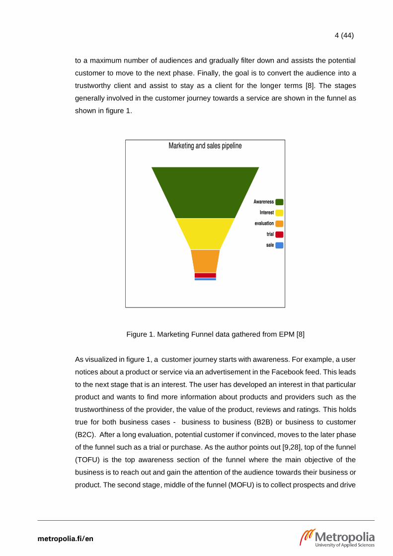
2.1.2 Marketing Funnel
For any business, it is essential to understand the customer experience or journey after
reaching out to the audience until converting that audience as a long-term trustworthy
buyer. This is well summarized in a visualization chart coined as marketing or purchasing
funnel as shown in figure 1. As the author stated, the point of the funnel is to reach out
4 (44)
to a maximum number of audiences and gradually filter down and assists the potential
customer to move to the next phase. Finally, the goal is to convert the audience into a
trustworthy client and assist to stay as a client for the longer terms [8]. The stages
generally involved in the customer journey towards a service are shown in the funnel as
shown in figure 1.
Figure 1. Marketing Funnel data gathered from EPM [8]
As visualized in figure 1, a customer journey starts with awareness. For example, a user
notices about a product or service via an advertisement in the Facebook feed. This leads
to the next stage that is an interest. The user has developed an interest in that particular
product and wants to find more information about products and providers such as the
trustworthiness of the provider, the value of the product, reviews and ratings. This holds
true for both business cases - business to business (B2B) or business to customer
(B2C). After a long evaluation, potential customer if convinced, moves to the later phase
of the funnel such as a trial or purchase. As the author points out [9,28], top of the funnel
(TOFU) is the top awareness section of the funnel where the main objective of the
business is to reach out and gain the attention of the audience towards their business or
product. The second stage, middle of the funnel (MOFU) is to collect prospects and drive
5 (44)
them towards the business resources such as a website. Finally, the bottom of the funnel
(BOFU) final stages of the funnel such as trial and sales where the business is focused
to convert potential customers into buyers. [9, 28.]
2.1.3 Marketing Key Performance Indicators
To build a cost-effective advertisement strategy, every stage of the customer journey is
measured and analyzed thoroughly. Various methods and metrics exist to measure
advertisement performance, however, those metrics can vary based on the end goals,
marketing strategy, stages, and advertisement platforms. For example, setting periodic
goals and analyzing the rate of goal completions is a great way to check if a marketing
strategy is effective as planned for web traffic analysis. To illustrate, few goals that can
be set and measured in the Google Analytics include the total purchases of a product,
the number of submitted contact information and the number of visitors to the website
[10].
A Key Performance Indicator (KPI), is a numeric measure that can be used to cross-
check, quantify and evaluate the efficiency of advertisement process from various
dimensions [3,216]. In marketing, monitoring those KPIs provides hidden and valuable
insights into the strategy, campaigns or advertisements. For Instance, few key KPIs for
web analytics include unique visitors, traffic, ROI, sessions, and conversion [11,4].
Amongst other KPIs, a Marketing lead is a potential customer that expresses interest
towards the brand, business or service. Similarly, a marketing qualified lead (MQL) is a
lead that is more likey to become a buyer. The qualification is based on the person's
activities and engagement on the website such as pages the person has viewed or
content the person has downloaded. [12.]
2.2 Predictive Analytics
Since human civilization, mankind had a special interest in knowing the future or
unknown events. Since then, several methods were practiced for forecasting and the
method were based on random guessing, judgmental analysis, astrology, religious and
cultural faith or pure instinct. One of the popular examples of the traditional technique
that is still practiced in some places is Chinese palmistry. The tradition is dated back to
6 (44)
(202BC - 9 AD) and it is a technique to predict a person's character, traits, health, wealth
or other attribute based on the pattern of one's palm lines [13].
With the vast amount of data availability and technological advancement, various tools,
and technologies have emerged over the decades that help to implement learning from
the available information to predict the future or unknown event. The learning is based
on the patterns and correlation found on the given data. Those tools and techniques
have become industry standards and widely practiced in various fields such as health
care, insurance, marketing, finance, entertainment, education, e-commerce, and
banking. For instance, Netflix integrates these techniques to recommend programs
based on the user interest [14,121]. Similarly, email service providers such as Gmail or
Outlook uses these techniques to filter down the spam emails using text analysis method.
As the author points out these techniques are interchangeably called 'Machine Learning',
'Artificial Intelligence', 'Data Mining', 'Forecasting' or 'Predictive Analytics'. However, the
outcome and underline theory remains the same and can be collectively referred to as
'Predictive analytics'. [15,1.]
Predictive Analytics is a broad term to describe the process of predicting the likelihood
of an unknown event based on patterns found in the available data by statistical and
analytical techniques such as data mining, statistical modeling, Machine Learning and
AI [15,2]. The process enables the user to extract trends, patterns, relationships and
correlation from the data that is not visible otherwise. Frequently, the unknow event is in
the future, however, the technique can be used to predict any occurrences. An example
of present and unknown event is diagnosis of diseases based on the given symptoms.
The technique can be applied to predict both continuous or discrete values. In all cases,
the underline theory is to find the relationship between independent and dependent
variables from available data and find out the most probable result for the unknown.
2.2.1 Artificial Intelligence (AI) and Machine Learning
The term AI was first coined in 1956 by John McCarthy when he invited a team of experts
for a workspace to discuss the concept of intelligent machines. Today, it is a generic
topic and several definitions can be found for AI. In general, AI can be broadly described
as the field of study that deals with mimicking cognitive behavior into the machines to
solve problems that require human intelligence such as self-learning, pattern recognition
7 (44)
and problem-solving. [16.] Modern AI tools and techniques have dramatically improved
the way humans interact with machines and the ability of a machine to learn and perform
the task that requires observation, learning and reasoning skills. Recently, AI has
assisted humans to develop a smart and intelligent application, common examples being
autonomous vehicles, customer service boots, financial assistance, image recognition,
speech recognition, and natural language processing.
Machine learning, a subset of AI is a technique that enables the machine to learn about
the pattern based on various algorithms, build a model to explain the relationship and
develop the capability for prediction [17,9]. As mentioned in section 2.2, the term
Machine Learning highly correlates with `Predictive Analytics` and has gained a lot of
popularity since the beginning of the 21st century. The following sections discuss detail
about various techniques for a machine to perform cognitive learning with examples of
most common supervised machine learning algorithms used in the case project.
2.2.2 Learning Techniques
Similar to human learning approaches, machine learning approaches differs based on
the data, the problem domain, and the expected outcomes. Generally, the learning
technique is classified into 4 methods: Supervised Learning, Unsupervised Learning,
Semi-Supervised Learning, and Reinforcement Learning.
Supervised Learning
In supervised learning methods, the algorithm is trained with fully labeled datasets where
each observation is provided with the result that the machine should learn to predict.
Here, the machine can learn based on the input-output example given in training sets
and maps the learning into a mathematical function that is applied to new data to
calculates the results [18].
8 (44)
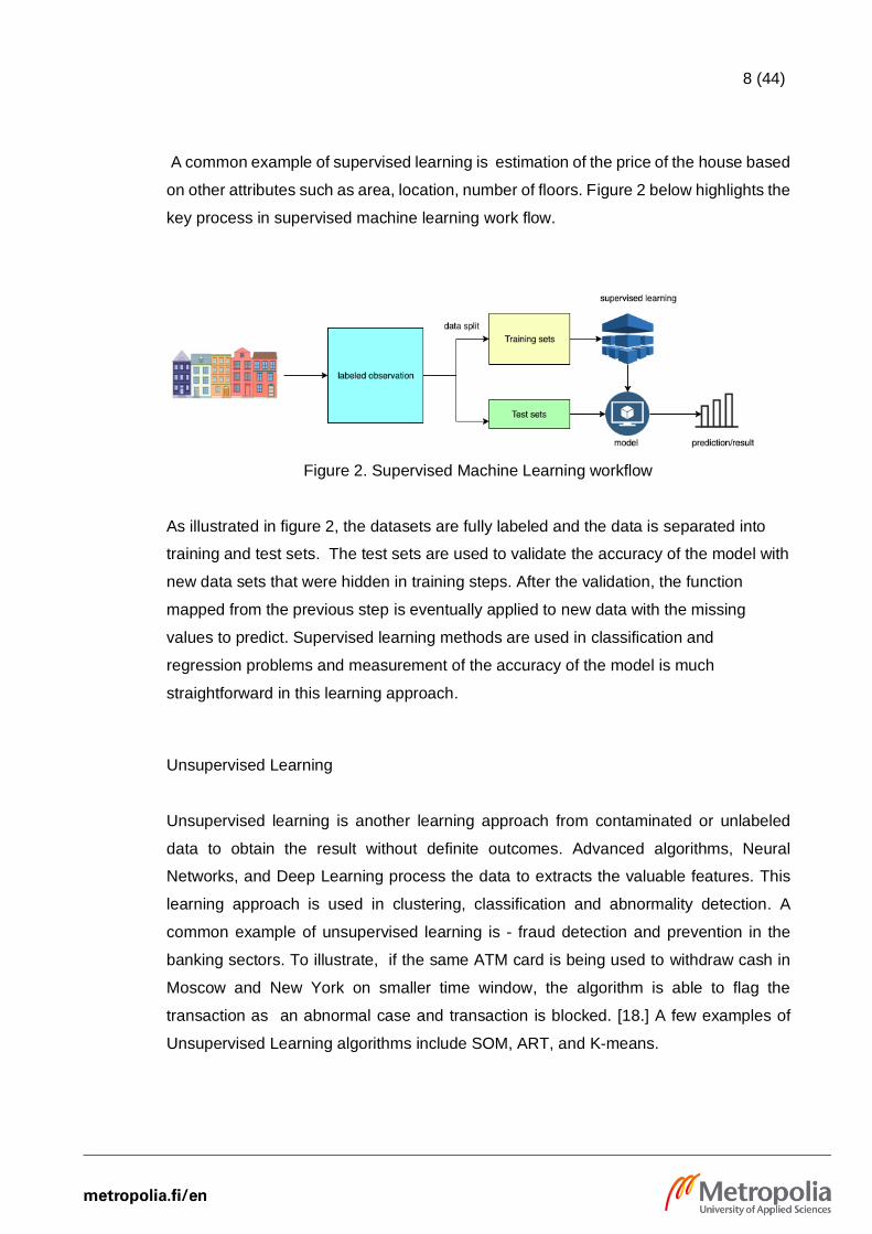
A common example of supervised learning is estimation of the price of the house based
on other attributes such as area, location, number of floors. Figure 2 below highlights the
key process in supervised machine learning work flow.
Figure 2. Supervised Machine Learning workflow
As illustrated in figure 2, the datasets are fully labeled and the data is separated into
training and test sets. The test sets are used to validate the accuracy of the model with
new data sets that were hidden in training steps. After the validation, the function
mapped from the previous step is eventually applied to new data with the missing
values to predict. Supervised learning methods are used in classification and
regression problems and measurement of the accuracy of the model is much
straightforward in this learning approach.
Unsupervised Learning
Unsupervised learning is another learning approach from contaminated or unlabeled
data to obtain the result without definite outcomes. Advanced algorithms, Neural
Networks, and Deep Learning process the data to extracts the valuable features. This
learning approach is used in clustering, classification and abnormality detection. A
common example of unsupervised learning is - fraud detection and prevention in the
banking sectors. To illustrate, if the same ATM card is being used to withdraw cash in
Moscow and New York on smaller time window, the algorithm is able to flag the
transaction as an abnormal case and transaction is blocked. [18.] A few examples of
Unsupervised Learning algorithms include SOM, ART, and K-means.
9 (44)
Reinforcement Learning
Reinforcement learning is an iterative learning approach from feedbacks and
experiences to find an optimal method to solve the problem. The learning agent is treated
with rewards while taking a step towards the target goals. Concurrently, it explores the
new approaches to solve the given problems. [18.] This learning approach is useful in
robotics and games where the more training is given to a machine, the better it becomes
performing a specific task. The most popular application of this learning approach is
AlphaGo Zero, a program created by London based AI company – DeepMind, that was
able to learn to play the game GO from scratch. Just after 40 days of self-learning, the
program was able to beat all other champions of Go player to be the best Go player in
the world. [19.]
2.2.3 Supervised Learning Algorithms
In supervised learning, classifications problems are the type of problem where the result
is a discrete value - set of a limited number of values. However, in a regression problem,
the result to be predicted is a continuous value. The classification problems can be a
binary classification – result with two possible values or multinomial classification – the
result contain more than two possible values. In the following section, common
supervised machine learning algorithms that are integrated to solve the problems for the
case project are discussed.
Linear Regression
Linear Regression is a simple and basic approach for preforming Predictive Analytics
and is a base for several advanced machine learning algorithms [20]. Usually, Linear
Regression is the first approach to Machine Learning for simpler problems and the
method is useful for forecasting quantitative response. The method works by finding out
the effect of sets of predictors on the result with various methods and forms the linear
equation.
10 (44)
For example, the linear relationship between total income and the amount of expense
can be defined with the equation as follows.
(1)
𝑌 = 𝛽0 + 𝛽1𝑋 + 𝜖
where Y = expense amount
X= income amount
β0 = coefficient - expense amount when income is 0
β1 = slope – change in expense amount for a unit change in income
ϵ = error terms
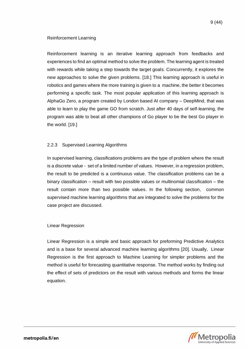
In the Simple Linear Regression equation above, the value of β1 and β0 is identified
that minimizes the deviation between the actual expense amount and expense amount
predicted by the equation based on the training data [20]. This can be visualized in
following plots with random data where the best fit is calculated with least squared error
methods and deviations are represented by red vertical lines.
Figure 3. Simple Linear Regression model plots with fitted values and residuals
Figure 3 includes three components of a simple Linear Regression model – observed
value, fitted value, and residuals. The blue line is fitted value - the estimated amount of
11 (44)
expense, green points represent observed value- the actual expense, and the red vertical
bar represents residuals - the difference between observed and predicted values.
Amongst various methods to find the best-fit regression equation, least squared error
method- a method to minimizes the sum of squared residuals is most common. In real-
life Regression problems, the result is explained by more than a single variable and that
is solved by multiple linear equations.
Logistic Regression
As explained in previous section, Linear Regression is limited to the problems with the
continuous response variable. The limitation is effectively solved by Logistic Regression
– a classification technique developed by statistician David Cox in 1958 [21]. The
method can take multiple predictors that explain the response value and calculates the
probability of categorical response. The response category can be binomial – only two
categorical response variables, Multinomial – more than two categorical response
variable or Ordinal – response variable can be ordered within a range [21].
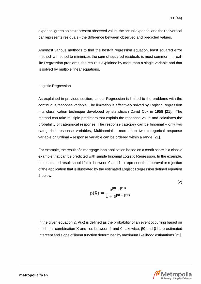
For example, the result of a mortgage loan application based on a credit score is a classic
example that can be predicted with simple binomial Logistic Regression. In the example,
the estimated result should fall in between 0 and 1 to represent the approval or rejection
of the application that is illustrated by the estimated Logistic Regression defined equation
2 below.
(2)
p(X) =eβ0 + β1X
1 + eβ0 + β1X
In the given equation 2, P(X) is defined as the probability of an event occurring based on
the linear combination X and lies between 1 and 0. Likewise, β0 and β1 are estimated
Intercept and slope of linear function determined by maximum likelihood estimations [21].
12 (44)
Decision Tree
Decision Tree is another supervised learning method to be used for both classification
and regression problems. In this method, the variable having the strongest association
with the response is chosen from various methods and the sample is partitioned based
on the chosen variable. The process is continued recursively with a binary partitioning
algorithm until certain criteria are met that results the final decision. Similar to the tree
data structure, a Decision Tree is composed of root nodes, decision nodes, branches,
leaf nodes and is placed upside down. The tree is started with the root node and
complete data-sets which is split into multiple subsets with certain conditions and the
process is continued up to the leaf of the tree with the outcome. [22, 175.]
Random Forests
Random Forests, as the name suggests, is an ensemble learning method that constructs
a large number of Decision Trees at the learning process and collective result from all
trees is gathered. For the regression problem, the final result is the average result of all
trees whereas for classification problems the the mode of the result is estimated as the
final result. Model based on Random Forest is much more accurate compared to single
Decision Trees as each tree is formed independently based on randomly sampled data.
Besides, it provides other significant advantages such as faster learning rate, avoids
overfitting, imputes the missing values and naturally handles both regression and
classification problems out of the box. [23,1.]
Naïve Bayes
Naïve Bayes is a simple linear machine learning technique but very effective in many
complex classification problems. The model is based on the conditional probability
theorem - Bayes’ theorem and assumes explanatory variables to be mutually
uncorrelated [24, 3]. The model outperforms other alternatives when the sample size is
less, and the number of features is more. The classifier is mostly used in text
classification, medical diagnosis and sentiment analysis such as filtering spam in email,
classifying customer sentiment based on reviews, categorizing news articles [24, 3].

13 (44)
As stated in the previous section, the model is based on the probability model formulated
by Statistician Thomas Bayes and it is called Bayes’ Theorem or alternatively Bayes’
Rule. It describes the rule to update the hypothesis based on the new evidence with joint
and conditional probabilities. The rule can be simplified as :
(3)
𝑝𝑜𝑠𝑡𝑒𝑟𝑖𝑜𝑟 𝑝𝑟𝑜𝑏𝑎𝑏𝑙𝑖𝑡𝑦 = 𝑐𝑜𝑛𝑑𝑖𝑡𝑖𝑜𝑛𝑎𝑙 𝑝𝑟𝑜𝑏𝑎𝑏𝑖𝑙𝑖𝑡𝑦 . 𝑝𝑟𝑖𝑜𝑟 𝑝𝑟𝑜𝑏𝑎𝑏𝑖𝑙𝑖𝑡𝑦
𝑒𝑣𝑖𝑑𝑒𝑛𝑐𝑒
In the above equation, posterior probability can be interpreted as the probability of
outcomes of a class given its observed properties such as the probability of a person to
be a woman based on long hair. Let’s Assume P(H) - the probability of a person being
woman, P(E) - the probability of the person having long hair and P(E|H) - the probability
of a person having long hair given that person is a woman. According to Bayes's
theorem, the posterior probability of the person to be a woman given that person has
long hair is given as follows [24,4].
(4)
𝑃(𝐻|𝐸) = 𝑝(𝐸|𝐻)
𝑃(𝐸) 𝑃(𝐻)
As mentioned in equation 4, based on Bayes' Theorem, the probability of a person
having long hair to be a woman is calculated based on prior known probabilities. First,
the probability of women having long hair is multiplied by the probability of any person
being a woman. Next, the result is divided by the probability of all persons having long
hair to obtain the result.
Artificial Neural Networks (ANNs)
Artificial Neural Networks are defined as robust non-linear machine learning algorithms
or function approximators that are inspired by biological neuron networks. The network
consists of several interconnected computational units or nodes known as neurons that
can process information autonomously. The results are then passed to other nodes from
14 (44)
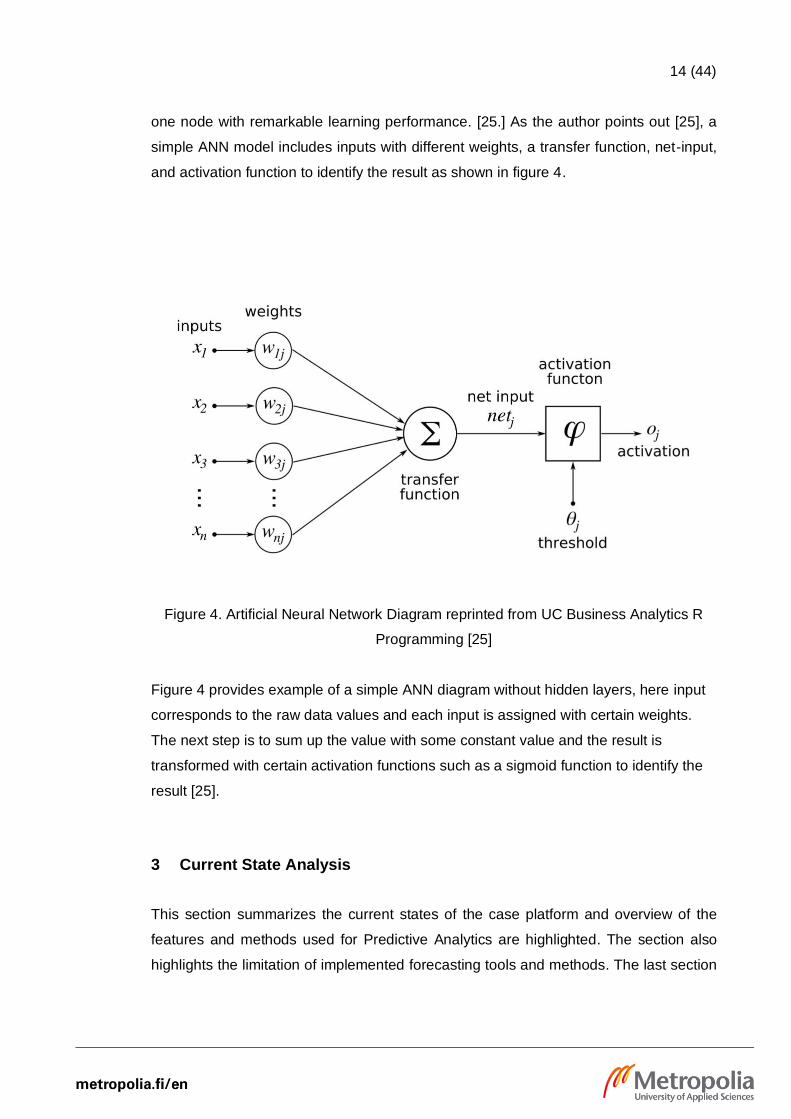
one node with remarkable learning performance. [25.] As the author points out [25], a
simple ANN model includes inputs with different weights, a transfer function, net-input,
and activation function to identify the result as shown in figure 4.
Figure 4. Artificial Neural Network Diagram reprinted from UC Business Analytics R
Programming [25]
Figure 4 provides example of a simple ANN diagram without hidden layers, here input
corresponds to the raw data values and each input is assigned with certain weights.
The next step is to sum up the value with some constant value and the result is
transformed with certain activation functions such as a sigmoid function to identify the
result [25].
3 Current State Analysis
This section summarizes the current states of the case platform and overview of the
features and methods used for Predictive Analytics are highlighted. The section also
highlights the limitation of implemented forecasting tools and methods. The last section
15 (44)
highlights the areas for improvement and points out the identified problem cases to be
implemented by the current project.
3.1 Inline Insight
The case platform for the project - Inline Insight, is a marketing automation or extract,
transform and load (ETL) tool that integrates with the number of digital marketing
platforms and CRM tools such as Google Ads, LinkedIn, Facebook, Twitter, HubSpot
and more. The platform extracts the data daily and harmonizes the KPIs across multiple
channels to a single table. Afterward, the data is loaded to the centralized reporting
system that makes it much convenient for comparitive analysis. Inline Insight also
supports data from organic and social channels such as the Instagram, LinkedIn and
Facebook pages to make it easier to compare the results based on organic and non-
organic sources. [26.]
The case platform is written in Python, R, JavaScript and is integrated with Azure cloud
services for storage, processing, and visualization of the data. The Azure services
includes Virtual Machine, Power BI reporting tools, Storage Account, SQL database, and
Azure Data lake. Users need to authorize permissions to fetch the data via a web
application. Afterward, the ETL written in Python extracts the data followed by data
transformation and processing in the R. The processed data is loaded to the Azure data
lake and eventually to the SQL server. The SQL Server provides the data source for
visualization tools such as the power BI reporting system or to the web application [26].
3.2 Advanced Analytics and Prediction
Beside from descriptive analytics, the case platform also provides advanced analytics
and simple prediction features such as recommendations, alerts, and forecasting. For
example. the platform recommends a marketer to increase or decrease the ad spend
amounts to maximizes cost per objective. For analytics and forecasting features, the
case platform uses basic forecasting formulas and forecasting models provided in power
BI. The basic prediction formulas include simple rolling average, naïve method and
seasonal naïve methods. Similarly, Inline insight adopts other forecasting methods
16 (44)
integrated with Power BI desktop for time series forecasting such as exponential
smoothing methods.
3.3 Limitation and issues
Predictive analytical features for the case platform are limited with the current
architecture and existing features include many accuracy drawbacks. Current
forecasting methods as mentioned in section 3.2 are limited to univariate time series
analysis and does not include external factors into the account [27, 1]. Due to limitations
with integrated models, the current predicted results are less accurate, and the platform
lacks additional features essentials for a competitive predictive analytical tool.
Similarly, The future roadmap for the platform is to turn into complete web service as a
(SaaS) service. SaaS can be defined as service provided over the internet that allows
the user to use the service without the need of maintaining or installing any software [28,
90]. However, the current implementation has proven to be against the philosophy of
SaaS. As a complete web service, the platform can not integrate with Power BI desktop
for advance analytics and prediction features and should migrate to other machine
learning tools and technologies.
3.4 Objectives
The major objective of the project is to build predictive models for two identified cases
listed below. During modeling, the project aim to explore and integrate various methods,
tools, and technologies into the case platform to streamline the new predictive features.
The following list provides the detail information of the cases identified to be solved with
the case project.
1. Sales case classification
In this case, the result of sales or deal cases in the pipeline is predicted and
scored with the probability of winning. The factors contributing to the result are
identified and include deal engagement and the activity of the contact and
17 (44)
company associated. Note that, in subsequent sections, the problem is labeled
as a deal classification case for better readability.
2. Marketing Lead prediction
These cases are regression problems and the metrics are predicted based on
the KPIs at the top of the funnel (TOFU) as explained in section 2.1.2. The
purpose is to predict key metrics - the total number of weekly website visitors,
Leads and MQLs gained. Theses cases are collectively referred to as Lead
prediction cases or regression problems.
4 Methods and Materials
The following section discusses the process, methods, tools, and technologies adopted
to carry out the project. The section also briefly explains the data used for predictive
modeling along with the application architecture. In the subsequent section, a detailed
workflow for implementation of the machine learning algorithm is discussed. Finally, the
last section highlights the accuracy evaluation methods for different machine learning
algorithms.
4.1 Tools and Technologies
For the implementation, various tools and packages provided in R and Python are
integrated. The next section provides an overview of R and python programming
language along with a short introduction to different machine learning tools used to
develop the project in R.
18 (44)
4.1.1 Python
Python is an open-source, high-level, general-purpose programming language that has
been widely used for data science in recent years [29]. As it provides a wide variety of
packages for making API calls and handling the large data sets, Python has been chosen
to extract the data from the various platforms for the case project. Further, Python data
analysis library- pandas is integrated to transform and store the API response to flat
format file such as CSV.
4.1.2 R
R is an open-source statistical programming language and environment for statistical
computing and graphics. The language was designed specifically to solve statistical
problems. R provides a variety of tools and techniques for statistical modeling,
classification, clustering, data mining, and graphics. [30.] In the context of the case
project, R has been utilized to perform machine learning and visualization tasks such as
data preparation, transformation, modeling and result visualization. The following section
shortly describes the various R libraries used for the tasks.
Rdatatable
Rdatatable or data.table is an extension of R tabular two-dimensional data structure -
data.frame with additional features such as high performance, fast speed, memory
efficiency, and concise syntax. As data.table is capable of storage and transformation of
large datasets in memory very fast, data for case project has been stored and processed
by data.table. [31.]
Caret
The caret package provides a common interface for various machine learning algorithms
for the development of predictive models. Additionally, it also provides a set of functions
to streamline the predictive analytics workflow such as data splitting, pre-processing,
feature engineering and resampling [32]. As of October 2019, it supports up to 238
algorithms and it is constantly growing [33]. Note that, Caret packages do not comes with
the packages for the different machine learning algorithms, however, users are prompted
19 (44)
to install only required libraries during run time. Functions provided by the caret packages
have been used in the case project to streamline the machine learning task for both
classification and regression problems.
CaretEnsemble
CaretEnsemble is a package in R for aggregating the result of multiple caret models.
The package helps to build ensemble models and provides three primary functions -
caretList, caretEnsemble, and caretStack. The first function is used to develop a list of
caret models and others are used to ensemble the models from the list. [34.]
4.2 Data
The data to execute the project belongs to the case company. Two sets of data has been
extracted to accomplish the modeling task that as discussed below.
For the Lead prediction case, Digital Marketing data has been extracted from the case
company’s advertisements and social accounts. The channels from the data were
extracted include - Instagram, LinkedIn, Google Analytics, Google Ads and HubSpot.
Overall, the last two years of data have been collected. The data comprises email
marketing, organic and paid advertisements and web traffic analytics. From each
channel, KPIs from the TOFU and MOFU are collected. For example, key metrics from
TOFU included social media KPIs such as user engagements, impressions, clicks,
shares, video views, reach, spend, ads objectives, target audience, advertisement type.
Similarly, Other metrics collected from web analytics platforms such as Google Analytics
and HubSpot included users, sessions, number of page views, bounces, conversions.
Similarly, For the classification problem, data included closed and ongoing deals in the
HubSpot sales pipeline since the beginning of 2017. In addition to deals, other data that
is suspected to have an impact on the result of the deal are also included such as
information about the contact and company deal is associated with. The predictors for
the deal result includes activities such as email, calls, meetings. Further, the data also
20 (44)
comprises detail information about the company and contact person with other online
activities such as the number of website visits, email clicks, email opens, page views.
4.3 Implementation
The following sections discuss the Machine Learning workflow and steps taken to build
predictive models for problems identified in section 3.4. The section briefly discusses the
data preparation task and machine learning workflow practiced in the project. Finally, the
performance of different models is evaluated in the subsequent section.
4.3.1 Data Preparation
Followed by data collection, data Preparation has been the starting step for Machine
Learning workflow. At first, the data is loaded into the R session as a list of data.table
and observed to gain a better insight into the data. With the understanding of the data,
the attributes with insignificant impact on the result are identified and removed to lower
down the number of variables. Afterward, each attribute is converted to correct data
types, the corrupt data is either fixed or removed and column names are renamed to be
more descriptive and according to the naming standard.
In supervised learning, in each record, the relevant information with the result should be
included. As discussed in section 4.2, the data for the case project is included in 7 and
16 different tables for classification and regression problem respectively. The next step
is to transform, clean and merge the relevant data into a single table.
4.3.2 Descriptive Analytics
At this stage, the distribution and quantitative insights for the attributes are summarized
with different measures and data is visually inspected. For the numerical attributes,
measures such as mean, median, mode, max, min, standard deviation, and variance are
summarized. The distribution of data that is visualized in several plots such as histogram,
correlogram or density plots. In contrast, for categorical attributes, class distribution is
observed and visually inspected with different charts such as pie charts or bar charts.

21 (44)
The data merged from various sources usually includes missing values. The ratio of
missing values is identified for each attribute and the attributes with a high ratio of missing
values - usually more than 75 percentages cannot be imputed effectively and are
removed.
4.3.3 Data Splitting and pre-processing
Prior to feeding data into the machine learning algorithms, the data is processed and
transformed into a more concise format. First, the data is split into training and test set
with a 75 to 25 percentages ratio. Training set consists of data that is fitted into the
Machine Learning algorithms to train the model. In contrast, the test set consists of data
for validation of the model’s accuracy. The function createDataParition from the Caret
package is used for the balanced partition of the data to preserve the overall distribution
of the response variable.
train_index <- createDataPartition(dt_model$dealstage, p = 0.75,
list = F)
Listing 1. Caret function to split the data
Listing 1 provides a Caret function for a balanced split of the data with 75 to 25
percentages ratio to be included in the training set and the test set.
22 (44)
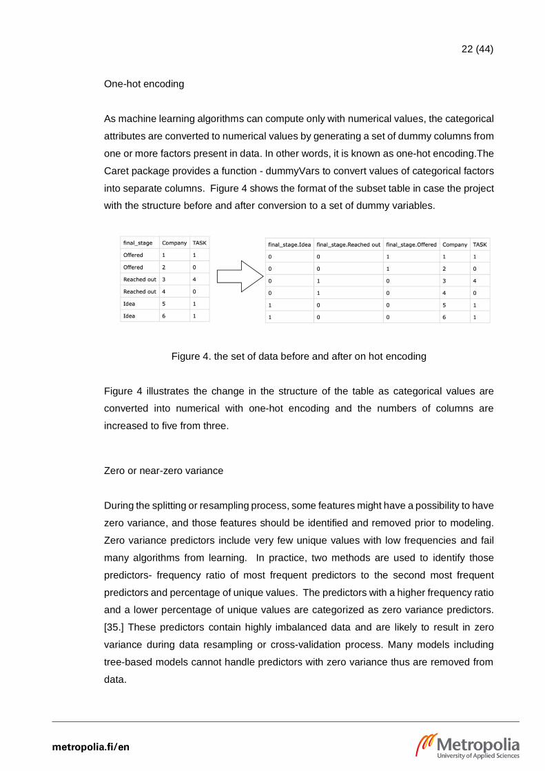
One-hot encoding
As machine learning algorithms can compute only with numerical values, the categorical
attributes are converted to numerical values by generating a set of dummy columns from
one or more factors present in data. In other words, it is known as one-hot encoding.The
Caret package provides a function - dummyVars to convert values of categorical factors
into separate columns. Figure 4 shows the format of the subset table in case the project
with the structure before and after conversion to a set of dummy variables.
Figure 4. the set of data before and after on hot encoding
Figure 4 illustrates the change in the structure of the table as categorical values are
converted into numerical with one-hot encoding and the numbers of columns are
increased to five from three.
Zero or near-zero variance
During the splitting or resampling process, some features might have a possibility to have
zero variance, and those features should be identified and removed prior to modeling.
Zero variance predictors include very few unique values with low frequencies and fail
many algorithms from learning. In practice, two methods are used to identify those
predictors- frequency ratio of most frequent predictors to the second most frequent
predictors and percentage of unique values. The predictors with a higher frequency ratio
and a lower percentage of unique values are categorized as zero variance predictors.
[35.] These predictors contain highly imbalanced data and are likely to result in zero
variance during data resampling or cross-validation process. Many models including
tree-based models cannot handle predictors with zero variance thus are removed from
data.
23 (44)
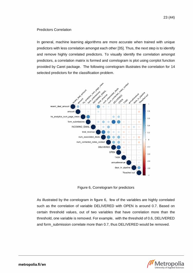
Predictors Correlation
In general, machine learning algorithms are more accurate when trained with unique
predictors with less correlation amongst each other [35]. Thus, the next step is to identify
and remove highly correlated predictors. To visually identify the correlation amongst
predictors, a correlation matrix is formed and correlogram is plot using corrplot function
provided by Caret package. The following correlogram illustrates the correlation for 14
selected predictors for the classification problem.
Figure 6, Correlogram for predictors
As illustrated by the correlogram in figure 6, few of the variables are highly correlated
such as the correlation of variable DELIVERED with OPEN is around 0.7. Based on
certain threshold values, out of two variables that have correlation more than the
threshold, one variable is removed. For example, with the threshold of 0.6, DELIVERED
and form_submission correlate more than 0.7, thus DELIVERED would be removed.
24 (44)
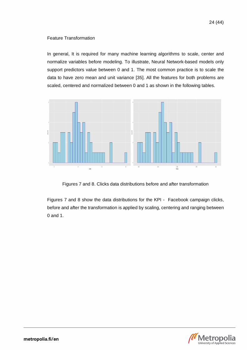
Feature Transformation
In general, It is required for many machine learning algorithms to scale, center and
normalize variables before modeling. To illustrate, Neural Network-based models only
support predictors value between 0 and 1. The most common practice is to scale the
data to have zero mean and unit variance [35]. All the features for both problems are
scaled, centered and normalized between 0 and 1 as shown in the following tables.
Figures 7 and 8. Clicks data distributions before and after transformation
Figures 7 and 8 show the data distributions for the KPI - Facebook campaign clicks,
before and after the transformation is applied by scaling, centering and ranging between
0 and 1.
25 (44)
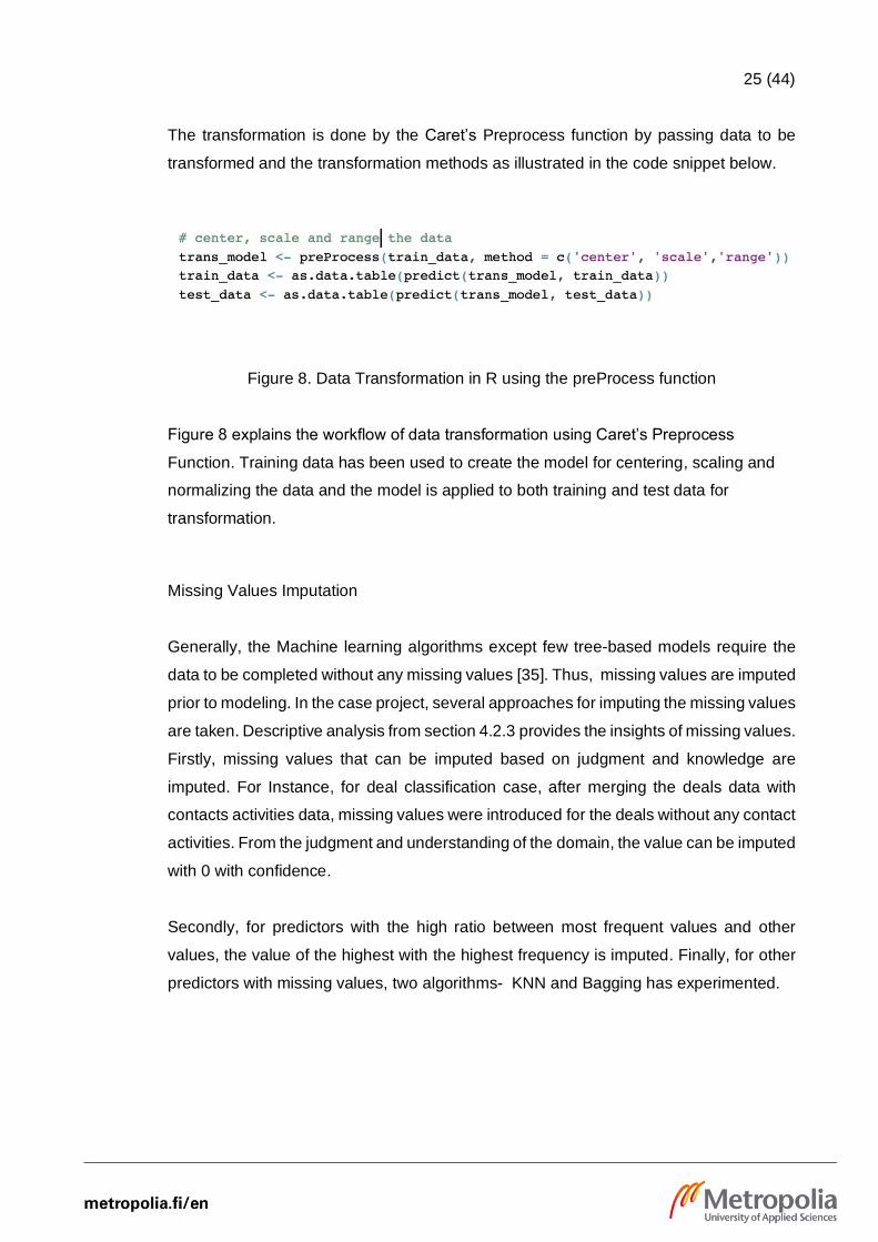
The transformation is done by the Caret’s Preprocess function by passing data to be
transformed and the transformation methods as illustrated in the code snippet below.
Figure 8. Data Transformation in R using the preProcess function
Figure 8 explains the workflow of data transformation using Caret’s Preprocess
Function. Training data has been used to create the model for centering, scaling and
normalizing the data and the model is applied to both training and test data for
transformation.
Missing Values Imputation
Generally, the Machine learning algorithms except few tree-based models require the
data to be completed without any missing values [35]. Thus, missing values are imputed
prior to modeling. In the case project, several approaches for imputing the missing values
are taken. Descriptive analysis from section 4.2.3 provides the insights of missing values.
Firstly, missing values that can be imputed based on judgment and knowledge are
imputed. For Instance, for deal classification case, after merging the deals data with
contacts activities data, missing values were introduced for the deals without any contact
activities. From the judgment and understanding of the domain, the value can be imputed
with 0 with confidence.
Secondly, for predictors with the high ratio between most frequent values and other
values, the value of the highest with the highest frequency is imputed. Finally, for other
predictors with missing values, two algorithms- KNN and Bagging has experimented.
26 (44)
4.3.4 Feature Selection
To achieve better accuracy with the model, only features with a significant impact on
results are selected, and other predictors that do not contribute to the results are
removed from the data. Despite manual approaches already taken identity significant
features in the previous sections, an automatic and streamline approach known as
recursive feature elimination is taken in the phase.
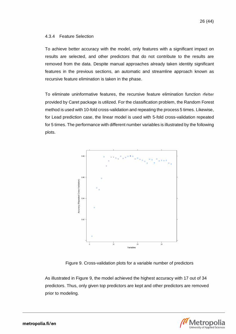
To eliminate uninformative features, the recursive feature elimination function rfeIter
provided by Caret package is utilized. For the classification problem, the Random Forest
method is used with 10-fold cross-validation and repeating the process 5 times. Likewise,
for Lead prediction case, the linear model is used with 5-fold cross-validation repeated
for 5 times. The performance with different number variables is illustrated by the following
plots.
Figure 9. Cross-validation plots for a variable number of predictors
As illustrated in Figure 9, the model achieved the highest accuracy with 17 out of 34
predictors. Thus, only given top predictors are kept and other predictors are removed
prior to modeling.
27 (44)
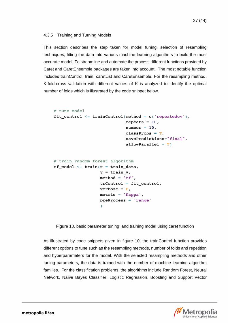
4.3.5 Training and Turning Models
This section describes the step taken for model tuning, selection of resampling
techniques, fitting the data into various machine learning algorithms to build the most
accurate model. To streamline and automate the process different functions provided by
Caret and CaretEnsemble packages are taken into account. The most notable function
includes trainControl, train, caretList and CaretEnsemble. For the resampling method,
K-fold-cross validation with different values of K is analyzed to identify the optimal
number of folds which is illustrated by the code snippet below.
Figure 10. basic parameter tuning and training model using caret function
As illustrated by code snippets given in figure 10, the trainControl function provides
different options to tune such as the resampling methods, number of folds and repetition
and hyperparameters for the model. With the selected resampling methods and other
tuning parameters, the data is trained with the number of machine learning algorithm
families. For the classification problems, the algorithms include Random Forest, Neural
Network, Naïve Bayes Classifier, Logistic Regression, Boosting and Support Vector
28 (44)
Machine. Similarly, for the Lead prediction case problem, the algorithms include Neural
Network, Linear Regression, Bayesian Linear models and Quantile Random Forest.
4.3.6 Ensemble Models
To maximize the accuracy of the machine learning models and reduce the bias, the
common practice is to ensemble models by combining the results from multiple
algorithms. Some of the algorithms used in the training and tuning sections are already
ensembled such as Random Forest or Boosting. However, to build a highly accurate
model, the most accurate algorithms that are identified from section 4.3.5 are ensembled.
In practice, R package caretEnsemble has been added to the project that provides a set
of functions that made it easier to ensemble the learning from two or more algorithms.
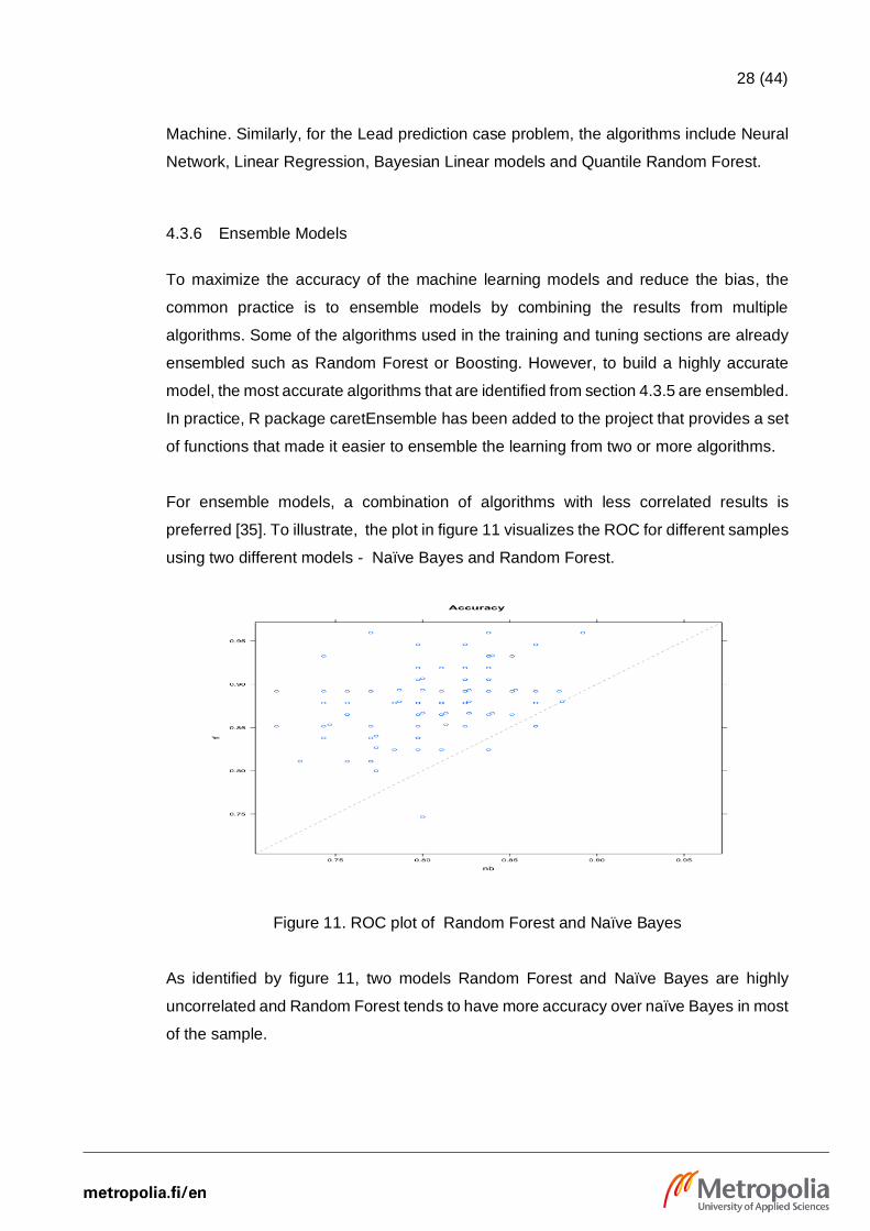
For ensemble models, a combination of algorithms with less correlated results is
preferred [35]. To illustrate, the plot in figure 11 visualizes the ROC for different samples
using two different models - Naïve Bayes and Random Forest.
Figure 11. ROC plot of Random Forest and Naïve Bayes
As identified by figure 11, two models Random Forest and Naïve Bayes are highly
uncorrelated and Random Forest tends to have more accuracy over naïve Bayes in most
of the sample.
29 (44)
4.4 Model Evaluation
To build highly accurate models, the model's significance and accuracy are evaluated
with various metrics and selection of metrics differs based on the response variable type.
For either case, the model result is summarized at first that provides the accuracy of the
model with the training data sets. Next, Accuracy of the model is cross-validate with the
result from test data. Following the prediction, outcomes are validated against the actuals
with a variety of evaluation metrics as summarized below.
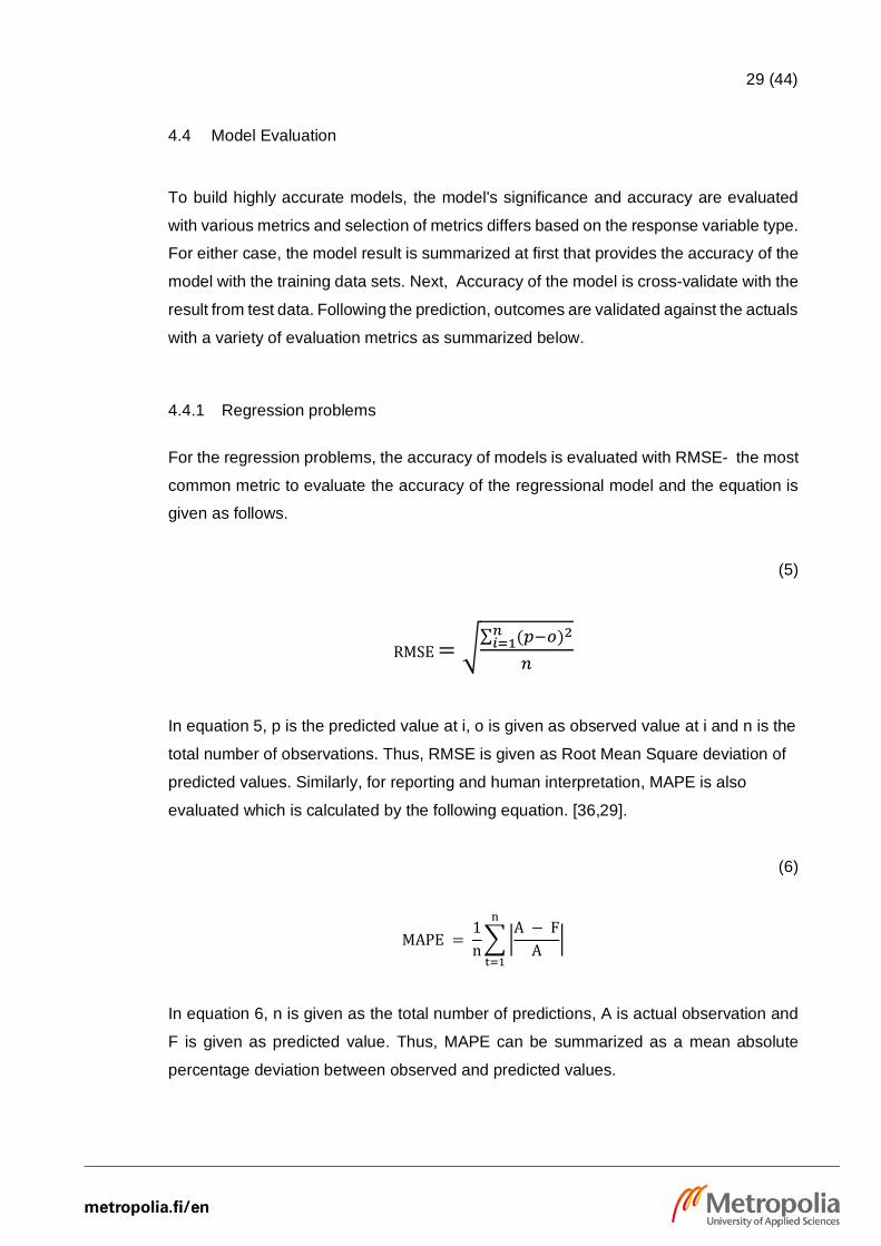
4.4.1 Regression problems
For the regression problems, the accuracy of models is evaluated with RMSE- the most
common metric to evaluate the accuracy of the regressional model and the equation is
given as follows.
(5)
RMSE = √∑ (𝑝−𝑜)2𝑛
𝑖=1
𝑛
In equation 5, p is the predicted value at i, o is given as observed value at i and n is the
total number of observations. Thus, RMSE is given as Root Mean Square deviation of
predicted values. Similarly, for reporting and human interpretation, MAPE is also
evaluated which is calculated by the following equation. [36,29].
(6)
MAPE = 1
n∑ |
A − F
A|
n
t=1
In equation 6, n is given as the total number of predictions, A is actual observation and
F is given as predicted value. Thus, MAPE can be summarized as a mean absolute
percentage deviation between observed and predicted values.

30 (44)
4.4.2 Classification problem
For classification problems, mostly three metrics are taken into account for accuracy
evaluation- Accuracy, Kappa and ROC and the value of all metric lies between 0 and 1.
Accuracy is the simplest and default metric to maximize in most machine learning models
with classification problems and is given as follows.
(7)
Accuracy = Number of correct prediction
Total number of predictions made
However, in most cases, the response class is not evenly distributed, and Accuracy is
not the most effective metric to evaluate the models. To illustrate, in the context of
classification problems in the case project, about 25 percentages of cases were won and
simply predicting all cases as lost gives 0.75 Accuracy that is very poor for predicting
won cases. To deal with the imbalance distribution of result class, Cohen’s kappa has
been used as an evaluation metric for classification models which is given as follows.
(8)
kappa = total accuracy − random accuracy
1 − random accuracy
As shown in equation 8, Kappa statistics takes observed accuracy by random chance
into account to have a more effective evaluation [37,147]. The model evaluation metrics
discussed for classification problems can be visualized in the confusion matrix that
shows cross-tabulation of observed and predicted classes as illustrated in the matrix
table below.
31 (44)
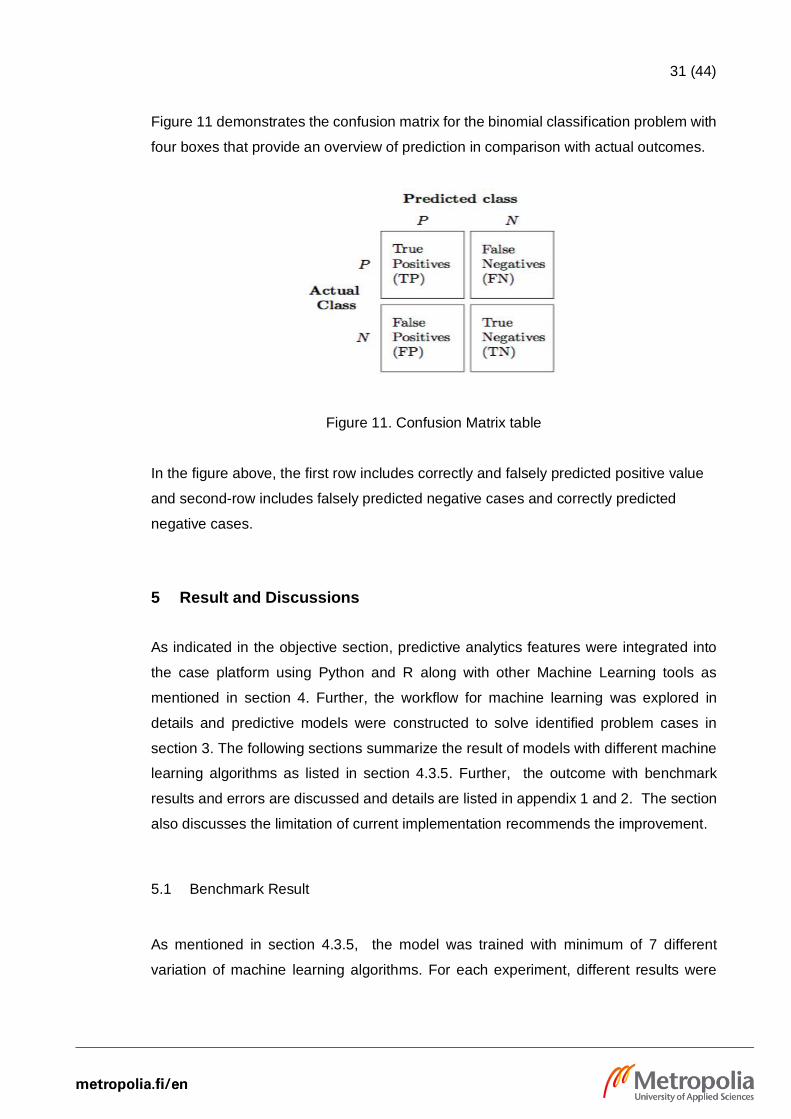
Figure 11 demonstrates the confusion matrix for the binomial classification problem with
four boxes that provide an overview of prediction in comparison with actual outcomes.
Figure 11. Confusion Matrix table
In the figure above, the first row includes correctly and falsely predicted positive value
and second-row includes falsely predicted negative cases and correctly predicted
negative cases.
5 Result and Discussions
As indicated in the objective section, predictive analytics features were integrated into
the case platform using Python and R along with other Machine Learning tools as
mentioned in section 4. Further, the workflow for machine learning was explored in
details and predictive models were constructed to solve identified problem cases in
section 3. The following sections summarize the result of models with different machine
learning algorithms as listed in section 4.3.5. Further, the outcome with benchmark
results and errors are discussed and details are listed in appendix 1 and 2. The section
also discusses the limitation of current implementation recommends the improvement.
5.1 Benchmark Result
As mentioned in section 4.3.5, the model was trained with minimum of 7 different
variation of machine learning algorithms. For each experiment, different results were
32 (44)
obtained that has been listed in appendixes 1 and 2 with different visualizations. The
Following sections provide an overview of the benchmark results.
5.1.1 Deal classification case
For the classification case, out of a total of 136 predictors, only 17 predictors were chosen
to be included in the models based on the feature selection technique discussed in the
section 4.3.4. For better interpretation, The chosen features along with the weight for
contribution are included in appendix 1 page 2. As bagging is computationally expensive
than the k-nearest neighbors (KNN) method to compute and no significant difference
was found with both approaches, thus KNN was chosen as the final imputation method.
In terms of algorithm, the data was trained using minimum of 5 different families of
machine learning algorithms and a couple of experiments were done using ensemble
models. For each machine learning algorithm, measured Accuracy, Kappa and AUC
values are in the appendix 1 page 1. As per the table, the model can be concluded as
highly accurate as more than 80 percentages of algorithms achieved more than 80
percentages of accuracy.
33 (44)
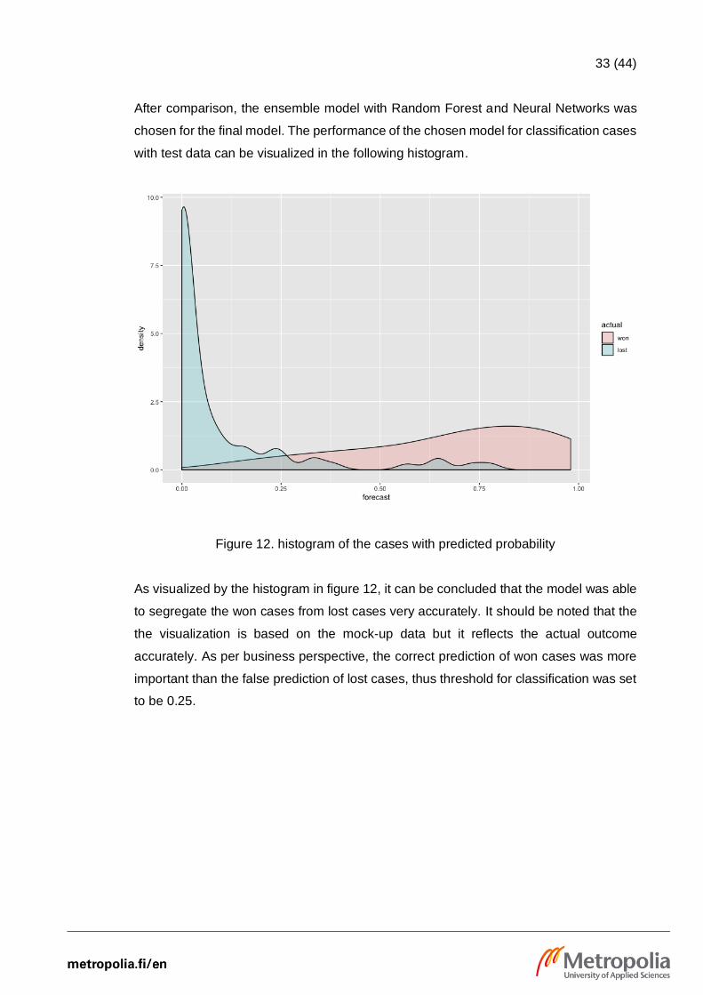
After comparison, the ensemble model with Random Forest and Neural Networks was
chosen for the final model. The performance of the chosen model for classification cases
with test data can be visualized in the following histogram.
Figure 12. histogram of the cases with predicted probability
As visualized by the histogram in figure 12, it can be concluded that the model was able
to segregate the won cases from lost cases very accurately. It should be noted that the
the visualization is based on the mock-up data but it reflects the actual outcome
accurately. As per business perspective, the correct prediction of won cases was more
important than the false prediction of lost cases, thus threshold for classification was set
to be 0.25.
34 (44)
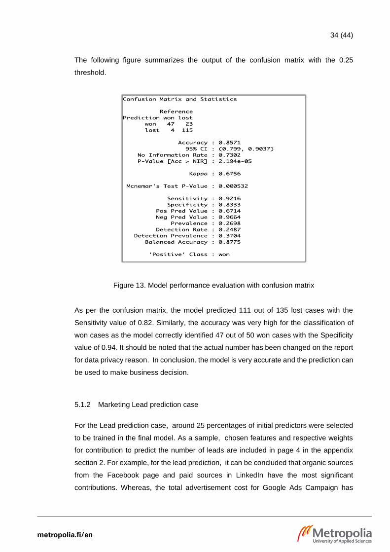
The following figure summarizes the output of the confusion matrix with the 0.25
threshold.
Figure 13. Model performance evaluation with confusion matrix
As per the confusion matrix, the model predicted 111 out of 135 lost cases with the
Sensitivity value of 0.82. Similarly, the accuracy was very high for the classification of
won cases as the model correctly identified 47 out of 50 won cases with the Specificity
value of 0.94. It should be noted that the actual number has been changed on the report
for data privacy reason. In conclusion. the model is very accurate and the prediction can
be used to make business decision.
5.1.2 Marketing Lead prediction case
For the Lead prediction case, around 25 percentages of initial predictors were selected
to be trained in the final model. As a sample, chosen features and respective weights
for contribution to predict the number of leads are included in page 4 in the appendix
section 2. For example, for the lead prediction, it can be concluded that organic sources
from the Facebook page and paid sources in LinkedIn have the most significant
contributions. Whereas, the total advertisement cost for Google Ads Campaign has
35 (44)
relatively less impact to the number leads collected. It should be noted that the test data
had included observed results with 0 values, thus RMSE was measured as a key metric
for the selection of the final algorithm.
The result of the Lead prediction case is listed in the table in appendix 2 pages 1,2 and
3. According to the tables, the performance of the model was found to be very accurate
for the prediction of the number of website visitors. For most cases, the average MAPE
value of all the algorithms is under 35 percentages other than Linear Regression and
BRNN.
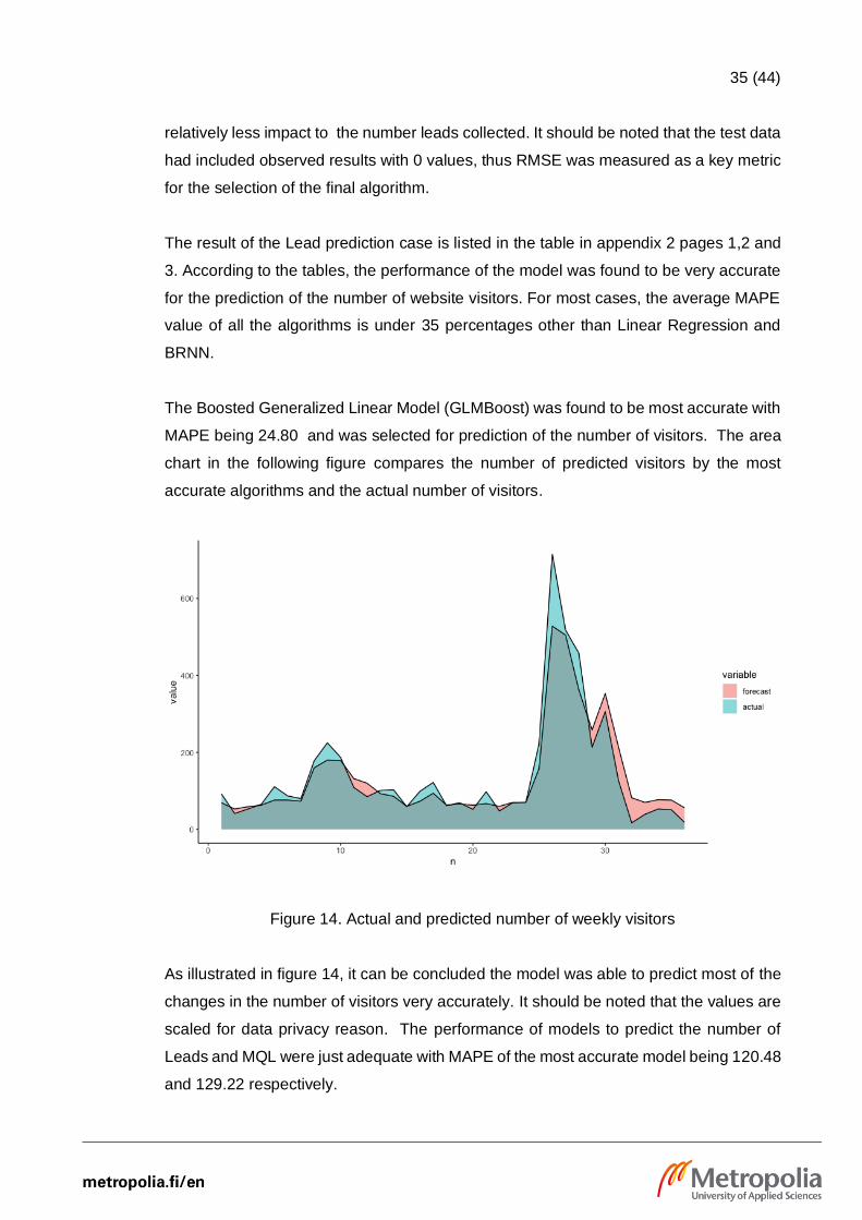
The Boosted Generalized Linear Model (GLMBoost) was found to be most accurate with
MAPE being 24.80 and was selected for prediction of the number of visitors. The area
chart in the following figure compares the number of predicted visitors by the most
accurate algorithms and the actual number of visitors.
Figure 14. Actual and predicted number of weekly visitors
As illustrated in figure 14, it can be concluded the model was able to predict most of the
changes in the number of visitors very accurately. It should be noted that the values are
scaled for data privacy reason. The performance of models to predict the number of
Leads and MQL were just adequate with MAPE of the most accurate model being 120.48
and 129.22 respectively.
36 (44)
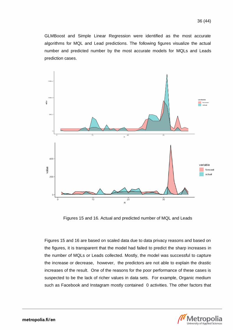
GLMBoost and Simple Linear Regression were identified as the most accurate
algorithms for MQL and Lead predictions. The following figures visualize the actual
number and predicted number by the most accurate models for MQLs and Leads
prediction cases.
Figures 15 and 16. Actual and predicted number of MQL and Leads
Figures 15 and 16 are based on scaled data due to data privacy reasons and based on
the figures, it is transparent that the model had failed to predict the sharp increases in
the number of MQLs or Leads collected. Mostly, the model was successful to capture
the increase or decrease, however, the predictors are not able to explain the drastic
increases of the result. One of the reasons for the poor performance of these cases is
suspected to be the lack of richer values in data sets. For example, Organic medium
such as Facebook and Instagram mostly contained 0 activities. The other factors that
37 (44)
can impact the MQLs and Leads are suspected to be the activities of the past weeks
which are yet to be incorporated into the models.
Overall, it can be concluded that the KPIs from the TOFU stage can explain the number
of visitors very accurately. For other KPIs, the predictors from TOFU explained the
outcome to some extent. However, the attributes that motivate for the conversion of
visitors into MQL or Leads should be identified and taken into account before using
results for business decision.
5.2 Further improvement
As identified in result section 5.1, the project achieved highly accurate results for two
cases out of four. However, for all cases, there are high scopes for improvement which
is discussed in this section. Firstly, hyperparameters should be tuned manually to
optimize the model's learning process. In addition to hyperparameter optimization, model
evaluation and selection process should be streamlined and the number of other
machine learning algorithms should be added into the platform. For example, it is
suggested to experiment with multi-layered based Neural Networks algorithms provided
by the R interface of Keras package.
For the regression problems, the model should be trained with the datasets collected
from various accounts with richer values. As non-actional predictions are not effective
value for the business, the implementation should be extended to forecast KPIs only
based on factors that advertisers or businesses have control over. For instance, the
prediction of leads solely based on owned and paid media that business have control
over can provide bigger values to the business as they have control over those factors.
As identified in section 3.3, the case platform included limitations to integrate advanced
predictive and forecasting features with the existing architecture. To overcome the
identified limitation, implementation is to be migrated from power BI to more powerful
and flexible machine learning tools. The existing simple forecasting methods should be
refactored with various advanced models and the best-fitting model should be selected
per features.
38 (44)
6 Conclusion and Summary
The project was carried out for a cloud-based, marketing automation, data driven
solution provider company - InlineMarket to integrate predictive capabilities to the
existing analytical ETL tool. The project was set out to explore and understand machine
learning workflow along with essentials of common machine learning algorithms.
The purpose of the project was to implement predictive models for two cases - prediction
of the number of weekly visitors, Leads and MQL for a business and forecasting the
result of sales cases in the pipeline. The data was extracted from social accounts, ads
accounts and Hubspot CRM account from case company. For data processing R
language was used and Machine learning workflow was based on the function and
standard provided by two R packages - Caret and CaretEnsemble.
For both problems, models were constructed with various machine learning algorithms
along with ensemble models to find out the most accurate model. From cross-validation
with test data, the result was found to be very accurate for classification problems.
Whereas for the regression problems, the model had accurate prediction only for the the
number of visitors but other predictions were just adequate.
In conclusion, the project was able to achieve all the objectives defined and was able to
discover a few insights that would not have been known otherwise. From the result, the
deals with faster stage transition and more past deals with the associated company were
more likely to be winned. For the case company, it was found that the number of weekly
achieved leads was highly explained by number activities on the Facebook page and
Linkedin ads. Similarly, it is concluded that current data is not able to fully predict the
Leads and investigation to identify other contributing factors that are suggested.
Further, it is recommended that the case company should not make any business
decisions based on current prediction for the Leads. However, Classification of deals
and prediction of website visitors can be used to make a business decision as they are
highly accurate. Similarly, current time series forecasting features using Power BI are
suggested to migrate to more advanced and flexible tools such as R programming
language. As the architecture for Predictive Analytics had been integrated into the case

39 (44)
platform, the integration of new predictive features are more straightforward and is
recommended.
40 (44)
References
1. The Economist. The world’s most valuable resource is no longer oil, but data
[online]. London, United Kingdom: The Economist; May 2017.
URL: https://www.economist.com/leaders/2017/05/06/the-worlds-most-valuable-
resource-is-no-longer-oil-but-data. Accessed 7 September 2019.
2. Domo.com. Domo Resource - Data Never Sleeps 5.0 [online].
URL: https://www.domo.com/learn/data-never-sleeps-5. Accessed 10
September 2019.
3. Chaffey D, Ellis-Chadwick F. Digital marketing. 5th ed. Harlow: Pearson; 2019.
4. Piñeiro-Otero T, Martínez-Rolán X. Understanding Digital Marketing—Basics and
Actions. Springer; September. p.37-74.
5. Customer Relationship Management [online]. Bain; April 2019.
URL: https://www.bain.com/insights/management-tools-customer-relationship-
management. Accessed October 1 2019.
6. CRM 101: What is CRM? [online]. Salesforce.com; 2019.
URL: https://www.salesforce.com/crm/what-is-crm/. Accessed 2 November
2019.
7. Frost A. Sales Pipelines: A Comprehensive Guide for Sales Leaders and Reps
[online]. Blog.hubspot.com; 2019.
URL: https://blog.hubspot.com/sales/sales-pipeline. Accessed 5 November
2019.
8. EPM. The Marketing Funnel Explained [online].
URL: https://expertprogrammanagement.com/2017/06/understand-the-
marketing-funnel. Accessed 4 October 2019
9. Nguyen N. A tool for digital communication implementation in the marketing
funnel. Helsinki, Finland: Arcada University of Applied Sciences; 2017
41 (44)
10. About goals - Analytics Help [online]. Support.google.com; 2019
URL: https://support.google.com/analytics/answer/1012040. Accessed 12
October 2019
11. Saura J, Palos-Sánchez P, Cerdá Suárez L. Understanding the Digital Marketing
Environment with KPIs and Web Analytics. Future Internet. 2017;9(4):76.
12. Kusinitz S. The Definition of a Marketing Qualified Lead [In Under 100 Words]
[online]. Blog.hubspot.com; 2019 [cited 20 November 2019].
URL: https://blog.hubspot.com/marketing/definition-marketing-qualified-lead-
mql-under-100-sr. Accessed 12 September 2019
13. Palm Reading – Guide & Basics of Hand Reading to Tell Fortune, Chinese
Palmistry [online]. Yourchineseastrology.com; 2019.
URL: https://www.yourchineseastrology.com/palmistry/. Accessed 12 October
2019.
14. Siegel ER. Predictive Analytics : the power to predict who will click, buy, lie or
die. Revised and Updated edition. Hoboken, New Jersey: Wiley; 2016.
15. Kuhn M, Johnson K. Applied Predictive Modeling. 2nd edition. New York:
Springer; 2016.
16. Marr B. The Key Definitions Of Artificial Intelligence (AI) That Explain Its
Importance [online]. Forbes; Feburary 2018.
URL: https://www.forbes.com/sites/bernardmarr/2018/02/14/the-key-definitions-
of-artificial-intelligence-ai-that-explain-its-importance. Accessed 9 15 October
2019.
17. Maini V, Sabri S. Machine learning for human. 1st ed. 2018.
18. SALIAN I. Supervised Vs. Unsupervised Learning [online]. The Official NVIDIA
Blog; August 2018.
URL: https://blogs.nvidia.com/blog/2018/08/02/supervised-unsupervised-
learning/. Accessed 12 October 2019.
42 (44)
19. Silver D, Hassabis D. AlphaGo Zero: Starting from scratch [online]. London,
United Kingdom: Deepmind; October 2017.
URL: https://deepmind.com/blog/article/alphago-zero-starting-scratch.
Accessed 13 October 2019.
20. Linear Regression · UC Business Analytics R Programming Guide [online].
Cincinnati, Ohio: University of Cincinnati; 2019
URL: http://uc-r.github.io/linear_regression. Accessed 16 September 2019.
21. Logistic Regression.· UC Business Analytics R Programming Guide [online].
Cincinnati, Ohio: University of Cincinnati; 2019.
URL: http://uc-r.github.io/logistic_regression. Accessed 16 November 2019.
22. Zhang Z. Decision tree modeling using R. Annals of Translational Medicine.
2016;4(15):275-275.
23. Cutler A, Cutler D, Stevens J. Random Forests. Ensemble Machine Learning.
2011;45:157-176.
24. Raschka S. Naive Bayes and Text Classification I - Introduction and Theory.
Cornell University; 2014.
25. Artificial Neural Network Fundamentals · UC Business Analytics R Programming
Guide [online]. Cincinnati, Ohio: University of Cincinnati; 2019.
URL: http://uc-r.github.io/ann_fundamentals. Accessed 16 November 2019.
26. Campaign Analytics | InlineInsight [online]. Inlineinsight.com; 2019
URL: https://www.inlineinsight.com/product/campaign-analytics.
Accessed 11 September 2019
27. Describing the forecasting models in Power View [online]. Microsoft PowerBI; 8
May 2014.
URL: https://powerbi.microsoft.com/pt-br/blog/describing-the-forecasting-
models-in-power-view. Accessed 8 October 2019.

43 (44)
28. Kulkarni G. Cloud Computing-Software as Service. International Journal of Cloud
Computing and Services Science (IJ-CLOSER). 2012;1(1).
29. What is Python? Executive Summary [online]. Python Software Foundation;
2019.
URL: https://www.python.org/doc/essays/blurb/. Accessed 26 October 2019.
30. R: What is R? [online]. R Foundation; 2019.
URL: https://www.r-project.org/about.html. Accessed 3 November 2019
31. Rdatatable/data.table [online]. GitHub; 2019.
URL: https://github.com/Rdatatable/data.table. Accessed 7 November 2019
32. Kuhn M. 5 Model Training and Tuning | The caret Package [online]. Caret
Documenation; March 2019.
URL: https://topepo.github.io/caret/model-training-and-tuning.html. Accessed 10
October 2019.
33. Kuhn M. Available Models | The caret Package [online]. Caret Documenation;
March 2019.
URL: https://topepo.github.io/caret/available-models.html. Accessed 6
November 2019.
34. Mayer Z. A Brief Introduction to caretEnsemble [online]. CaretEnsemble
Documenation; January 2016.
URL: https://cran.r-
project.org/web/packages/caretEnsemble/vignettes/caretEnsemble-intro.html.
Accessed 6 November 2019.
35. Kuhn M. 3 Pre-Processing | The caret Package [online]. Caret Documenation;
March 2019.
URL: https://topepo.github.io/caret/pre-processing.html. Accessed 6 November
2019

44 (44)
36. Hyndman R, Athanasopoulos G. Forecasting Priciples and Practice. Heathmont,
Vic: OTexts; 2018.
37. Sun S. Meta-analysis of Cohen's kappa. Health Services & Outcomes Research
Methodology 2011 12;11(3-4):145-163
Appendix 1
1 (2)
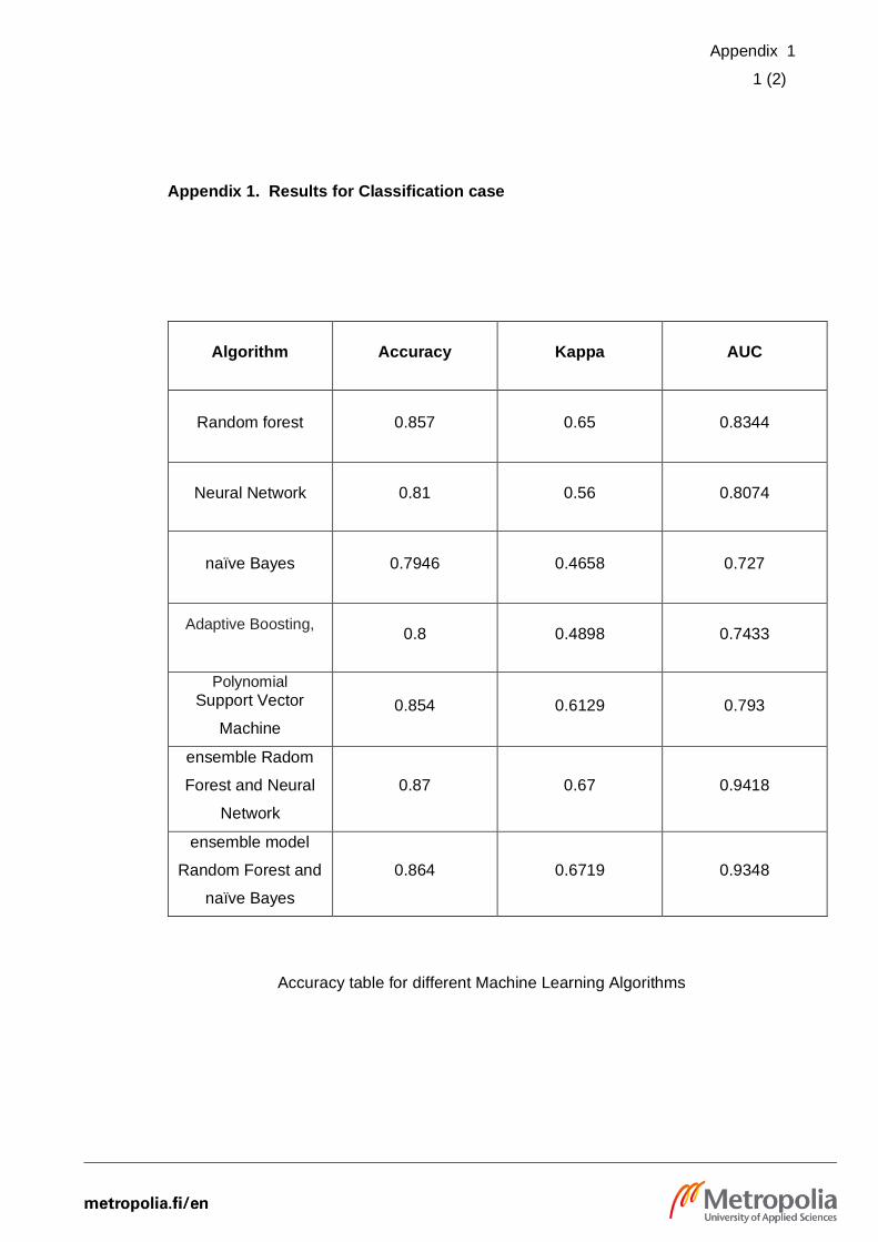
Appendix 1. Results for Classification case
Algorithm Accuracy Kappa AUC
Random forest 0.857 0.65 0.8344
Neural Network 0.81 0.56 0.8074
naïve Bayes 0.7946 0.4658 0.727
Adaptive Boosting,
0.8 0.4898 0.7433
Polynomial Support Vector
Machine
0.854 0.6129 0.793
ensemble Radom
Forest and Neural
Network
0.87 0.67 0.9418
ensemble model
Random Forest and
naïve Bayes
0.864 0.6719 0.9348
Accuracy table for different Machine Learning Algorithms
Appendix 1
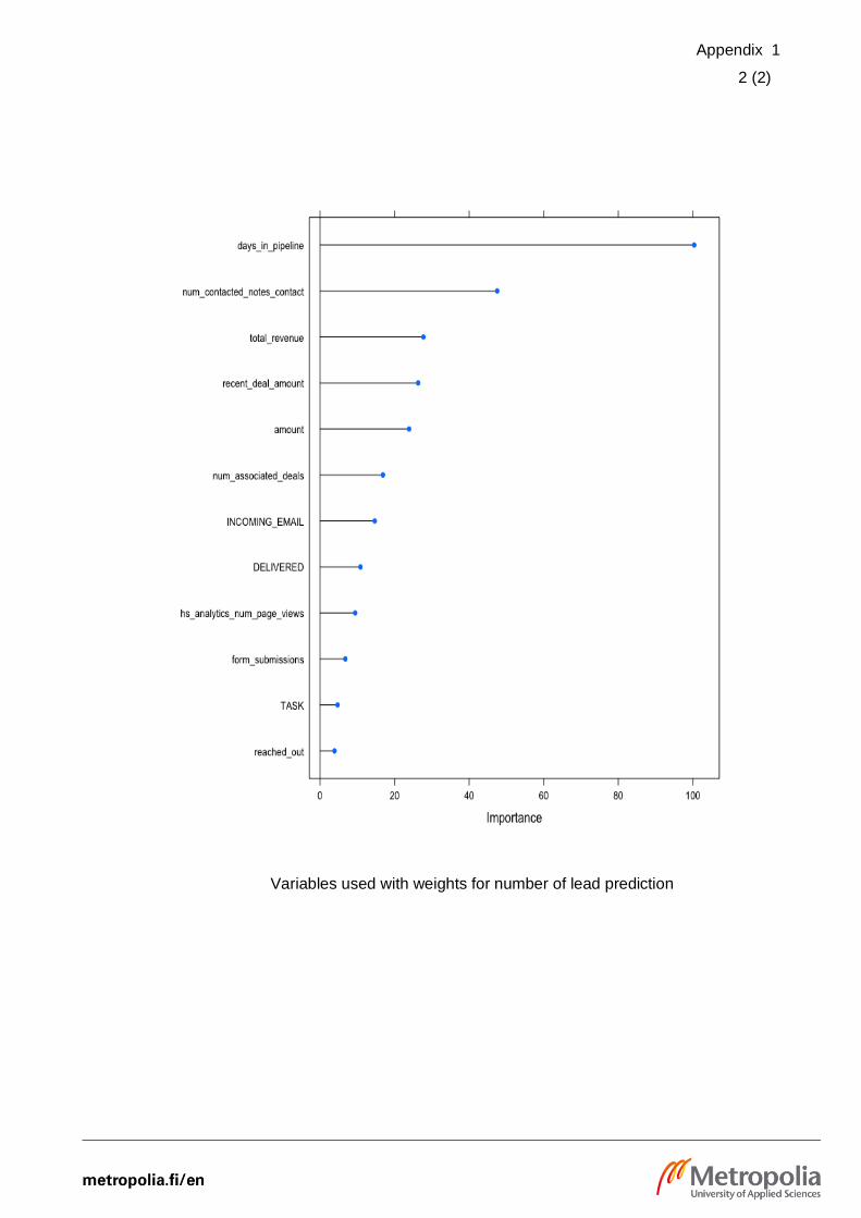
2 (2)
Variables used with weights for number of lead prediction
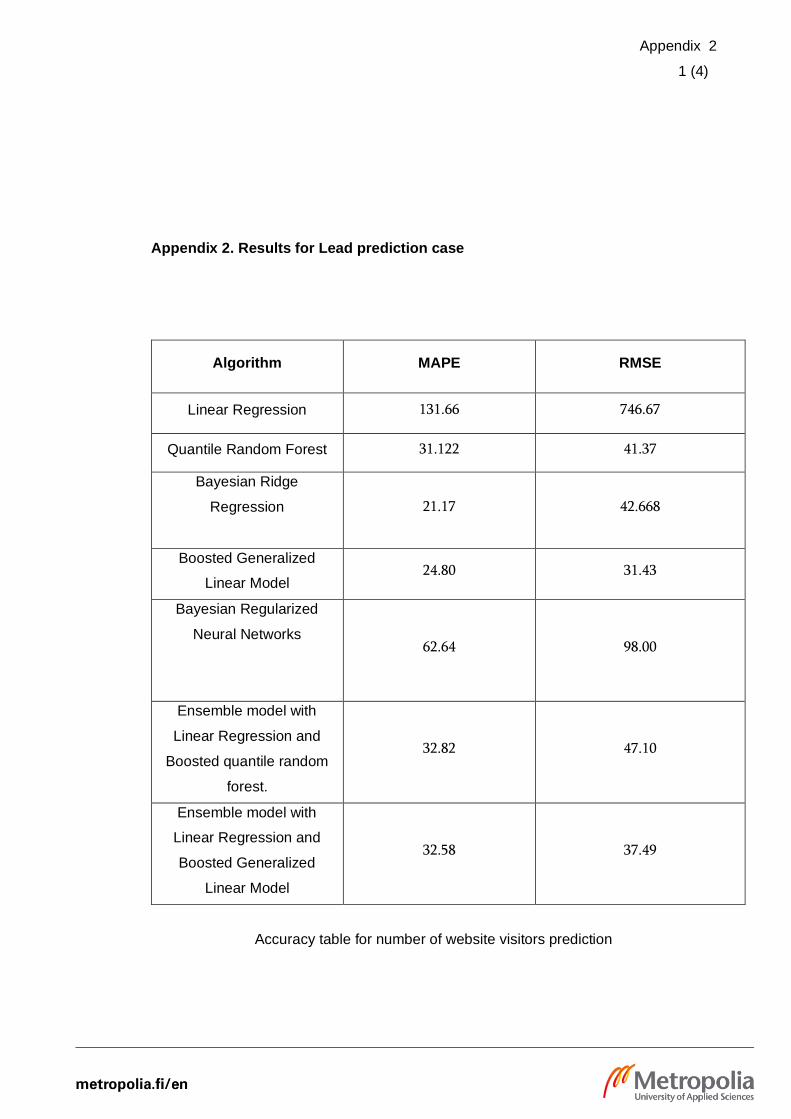
Appendix 2
1 (4)
Appendix 2. Results for Lead prediction case
Algorithm MAPE RMSE
Linear Regression 131.66 746.67
Quantile Random Forest 31.122 41.37
Bayesian Ridge
Regression
21.17 42.668
Boosted Generalized
Linear Model 24.80 31.43
Bayesian Regularized
Neural Networks
62.64 98.00
Ensemble model with
Linear Regression and
Boosted quantile random
forest.
32.82 47.10
Ensemble model with
Linear Regression and
Boosted Generalized
Linear Model
32.58 37.49
Accuracy table for number of website visitors prediction
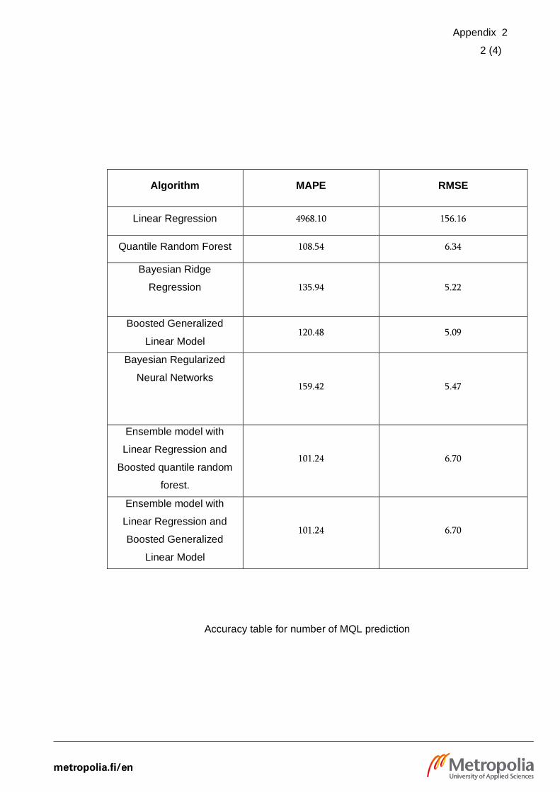
Appendix 2
2 (4)
Algorithm MAPE RMSE
Linear Regression 4968.10 156.16
Quantile Random Forest 108.54 6.34
Bayesian Ridge
Regression
135.94 5.22
Boosted Generalized
Linear Model 120.48 5.09
Bayesian Regularized
Neural Networks
159.42 5.47
Ensemble model with
Linear Regression and
Boosted quantile random
forest.
101.24 6.70
Ensemble model with
Linear Regression and
Boosted Generalized
Linear Model
101.24 6.70
Accuracy table for number of MQL prediction
Appendix 2
3 (4)
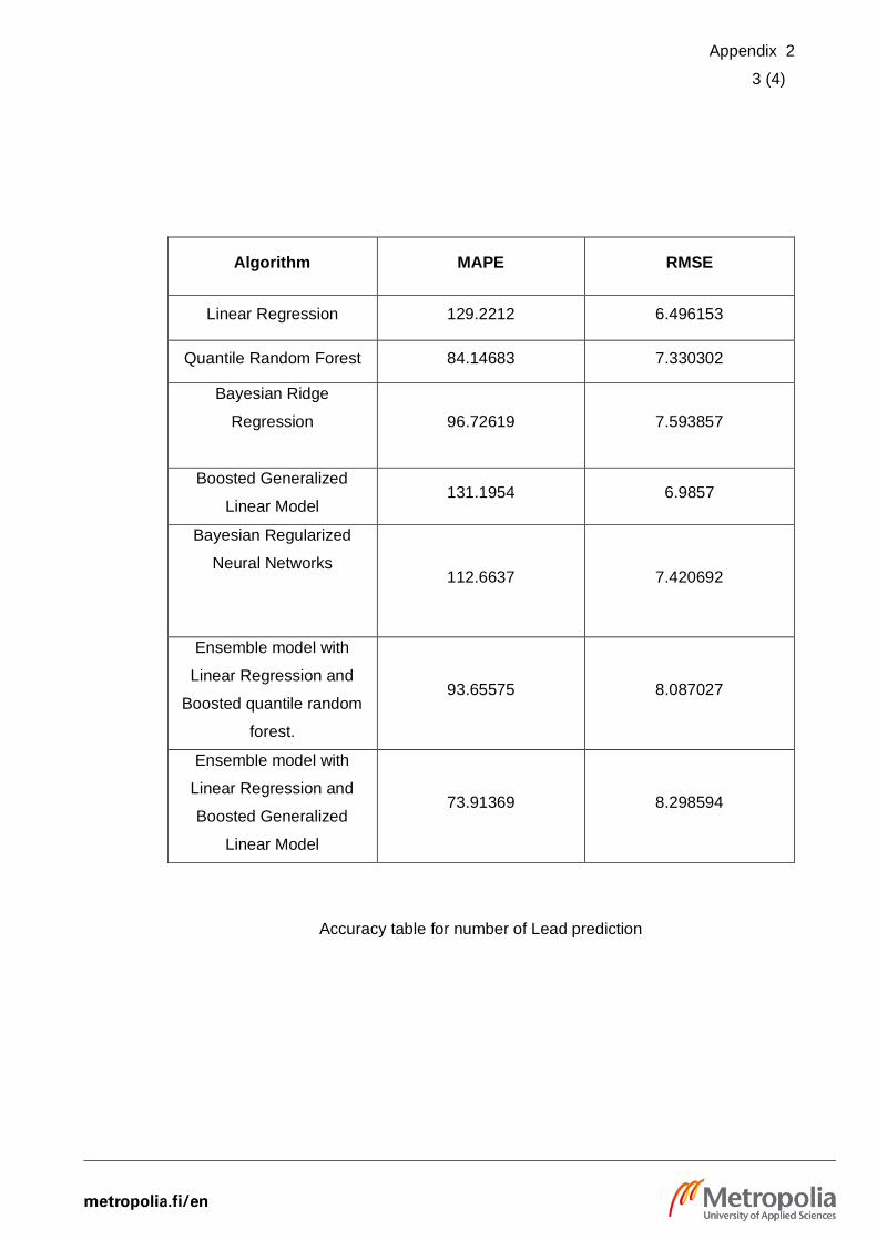
Algorithm MAPE RMSE
Linear Regression 129.2212 6.496153
Quantile Random Forest 84.14683 7.330302
Bayesian Ridge
Regression
96.72619 7.593857
Boosted Generalized
Linear Model 131.1954 6.9857
Bayesian Regularized
Neural Networks
112.6637 7.420692
Ensemble model with
Linear Regression and
Boosted quantile random
forest.
93.65575 8.087027
Ensemble model with
Linear Regression and
Boosted Generalized
Linear Model
73.91369 8.298594
Accuracy table for number of Lead prediction
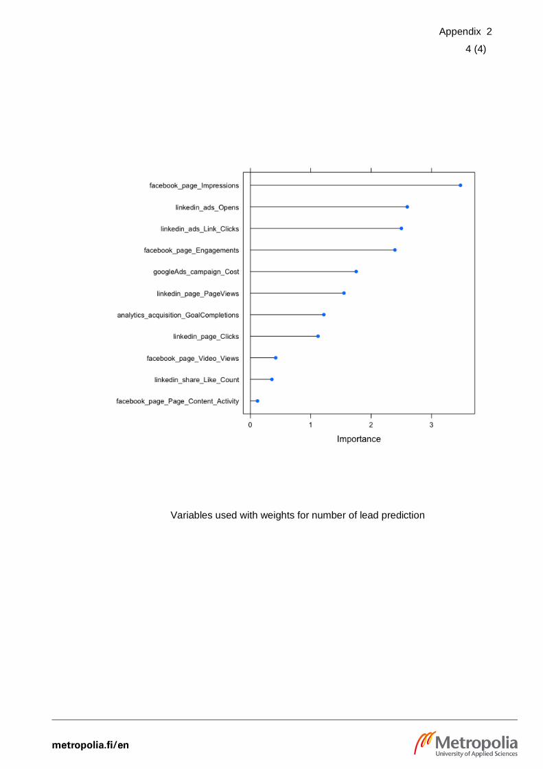
Appendix 2
4 (4)
Variables used with weights for number of lead prediction