Predictions West Nile Virus risk in the North

1

WAGENINGEN UNIVERSITEIT/

WAGENINGEN UNIVERSITY

LABORATORIUM VOOR ENTOMOLOGIE/

LABORATORY OF ENTOMOLOGY

Predictions of West Nile Virus risk associated with

Culex pipiens in North-West of Europe

MAS 800506888100

Quantitative Veterinary Epidemiology -

Entomology THESIS 60 ECTS No.:…08-05…………………. Naam/Name:…VIENNET Elvina……….. Periode/Period:…March 07-February 08…….. 1e Examinator:……Mart de Jong…… 2e Examinator:……Willem Takken…

2

SUMMARY ................................................................................................................................ 4 FIRST PART:.............................................................................................................................. 5 INTRODUCTION....................................................................................................................... 5 WEST NILE VIRUS IN THE WORLD ..................................................................................... 6

I. Retrospective on the West Nile Virus ............................................................................ 6 II. Epidemiology of West Nile Virus .................................................................................. 7 II.1 Introduction of WNV ..................................................................................................... 7 • Natural hosts of the West Nile virus – birds................................................................... 7 II.2 Amplification of WNV................................................................................................... 7 • Vectors of the virus – mainly mosquitoes ...................................................................... 7 • Transmission to the hosts – (mammals and humans) .....................................................8 III. Risk infection model for the West Nile virus................................................................. 8 • Transmission and vectorial capacity .............................................................................. 9

A POTENTIAL VECTOR ....................................................................................................... 10 • Presentation of the Culex pipiens pipiens .................................................................... 10 • Sources for adult feeding and host seeking behavior ................................................... 10

SECOND PART:....................................................................................................................... 12 MATERIEL AND METHODS................................................................................................. 12

EPIDEMIOLOGY.................................................................................................................. 13 WHICH MODEL TO USE AS A STARTING POINT FOR THE MODELLING OF WNV IN THE NORTH-WEST OF EUROPE?................................................................................ 13

I. Building a WNV model suitable for the North West of Europe .................................... 13 I.1 What about the existing WNV models? ....................................................................... 13 I.2 Can those models be used to predict WNV outbreaks in North-West Europe? ........... 14 I.3 What are the most important parameters to determine WNV transmission and risks for dead-end hosts? ...................................................................................................................... 15 I.4 Risk index for the West Nile virus ............................................................................... 16 I.5 West Nile virus model formulation .............................................................................. 18 I.6 Existence and stability equilibrium .............................................................................. 21 I.7 Test of credibility of the model .................................................................................... 23 ENTOMOLOGY.................................................................................................................... 26 The ecology of Culex pipiens pipiens in The Netherlands .................................................... 26

I. Field experiment: Population dynamics of Culex pipiens pipiens in different habitats . 26 I.1 Study area and environment ......................................................................................... 26 I.2 Mosquitoes ................................................................................................................... 28 I.3 Climate and vegetation................................................................................................. 30 I.4 Bird and animal density................................................................................................ 32 I.5 Timetable of the field experiment ................................................................................ 32

II. Laboratory experiment: Temperature effect on developmental time and survival rates 32 Experimental set-up and procedure........................................................................................ 32

III. Data analysis ................................................................................................................ 34 III.1 Field experiment data analysis ..................................................................................... 34 III.1.1 Environmental conditions.................................................................................... 34 III.1.2 Mosquito collection per area ............................................................................... 35 III.1.3 Culex pipiens adult density.................................................................................. 35 III.1.4 Culex pipiens larval density................................................................................. 36 III.1.5 Correlation between larval and adult C. pipiens.................................................. 36 III.2 Temperature effect on developmental time and survival rate ......................................36 III.2.1 Temperature effect on developmental time ......................................................... 36 III.2.2 Temperature effect on survival rates ................................................................... 36 III.2.3 Winglength/temperature correlation .................................................................... 36

THIRD PART: .......................................................................................................................... 38 RESULTS.................................................................................................................................. 38

ENTOMOLOGY.................................................................................................................... 39 I. Field studies.................................................................................................................. 39

I.1 Environmental conditions............................................................................................. 39

3

I.1.1 Meteorology ................................................................................................................. 39 I.1.2 Vegetation .................................................................................................................... 40 I.1.3 Bird and animal populations......................................................................................... 41 I.2 Adult collections (all species) ...................................................................................... 42 I.3 Culex pipiens collections per trap ................................................................................ 45 I.4 Larvae of Culex pipiens per study breeding site.......................................................... 49 I.5 Adult and larval density correlation ............................................................................. 52

II. Laboratory studies ........................................................................................................ 54 II.1 Temperature effect on developmental time and survival rates..................................... 54 II.1.1 Temperature effect on developmental time.................................................................. 54 II.1.2 Temperature effect on survival rates ............................................................................ 55 II.1.3 Wings length/temperature correlation .......................................................................... 55 II.2 Temperature effect on winglength................................................................................ 59 EPIDEMIOLOGY.................................................................................................................. 60

I. WNV model analysis ................................................................................................... 60 II. WNV model predictions............................................................................................... 63 FOURTH PART:....................................................................................................................... 65 DISCUSSION AND CONCLUSIONS..................................................................................... 65

EPIDEMIOLOGY.................................................................................................................. 66 • Public Health implications ........................................................................................... 67 • Future perspectives....................................................................................................... 67

ENTOMOLOGY.................................................................................................................... 68 REFERENCES.......................................................................................................................... 70 ANNEX..................................................................................................................................... 77

4

SUMMARY West Nile Virus (WNV), an emergent arbovirus, is a mosquito-borne flaviviral infection transmitted in natural cycles by vectors (mosquitoes, particularly Culex species but also Aedes species), among reservoir hosts (birds) and also occasionally to incidental dead-end hosts (humans and horses). West Nile virus (WNV) was first discovered in 1937 in the blood of a native woman of the West Nile province of Uganda (Smithburn et al. 1940). In the beginning of the 1960’s, WNV is considered as an arboviral pathogen of humans causing normally asymptomatic to mild diseases but which causes rarely serious neurological syndromes. The virus occurred in the Mediterranean Basin (Egypt, Maghreb, South of Europe, Near East), in Sub-Saharan Africa, in Madagascar, in Europe, and from Asia Minor to India, showing its ability for adaptation to different bird species and vectors (Murgue et al. 2001). Until the beginning of the 1990’s, WNV is still considered to be only occasionally highly pathogenic. But in the ten years that followed, West Nile Virus showed its capacity to spark off many hundred meningoencephaliti epidemics in the Mediterranean Basin and principally in the United-States. Indeed in 1999, West Nile Virus jumped oceans and arrived in the USA, where since then many people, have died (Marfin et al. 2001).Since then, major outbreaks and sporadic cases have been reported in Africa, Asia, the Middle-East and in Europe: Italy 1998; France 2000, 2003, 2004, 2006 (Balenghien 2006); Hungary 2004; Romania 1996, 1997, 1998, 1999, 2000 (Ceianu et al. 2001) and Czech Republic 1997 (Hubalek et al. 1999), 1999 (Rogers 2006). Therefore, WNV has recently become a major public health and veterinary concern. Due to the persistence of many (new) infectious diseases in humans, animals, or plants, there was an increase in theoretical research using models to understand the epidemiology of infectious diseases. Indeed, such models can be used to help with making decisions regarding public health, social and ecological issues.

Nowadays several groups try to develop an epidemiological model for WNV. Mathematical models for this vector-transmitted disease with cross-infection between birds and mosquitoes have been recently proposed with the purpose of predicting disease dynamics and evaluating possible control methods. Nevertheless, the literature on the mathematical modelling of WNV transmission is rather limited and most of the research has been done in USA, whereas in Europe they are still ongoing. An example is the study of Thomas et al. (2001) who presented a model for WNV to target its effects on New York City and to propose an amount of necessary spraying to eradicate the virus and also the research from Wonham et al. (2004) who present a single-season ordinary differential equation model for WNV transmission in the mosquito-bird population.

At the present time, this disease is not a public health problem in Europe; nevertheless in the USA, outbreaks tell us to take seriously into account the health risk of WNV. According to the Centers for Diseases Control and Prevention (CDC), the cumulative number of human disease cases in USA is 3576 (updated February 5, 2008). Many scientific questions still need to be answered concerning, on the one hand, birds’ species and the vectors involved in the transmission and, on the second hand, the relation between the environment and the transmission.

The aim of this study is to develop a dynamic model for WNV and use this model to predict disease dynamics and evaluating possible intervention and control methods in North-West of Europe. The model has been verified with field data on Culex pipiens pipiens and biological growth data from laboratory studies, and show the importance of a good estimation of the vector density and biting rate.

Keywords: West Nile virus; Culex pipiens pipiens; Model; developmental time

5

FIRST PART:

INTRODUCTION

6

WEST NILE VIRUS IN THE WORLD I. Retrospective on the West Nile Virus

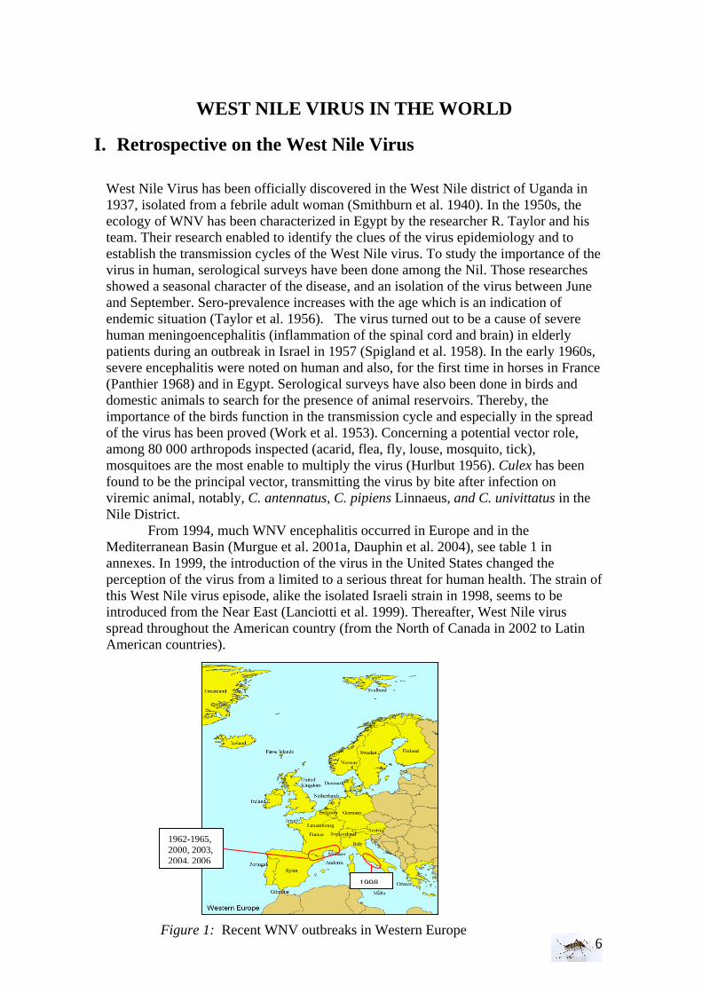
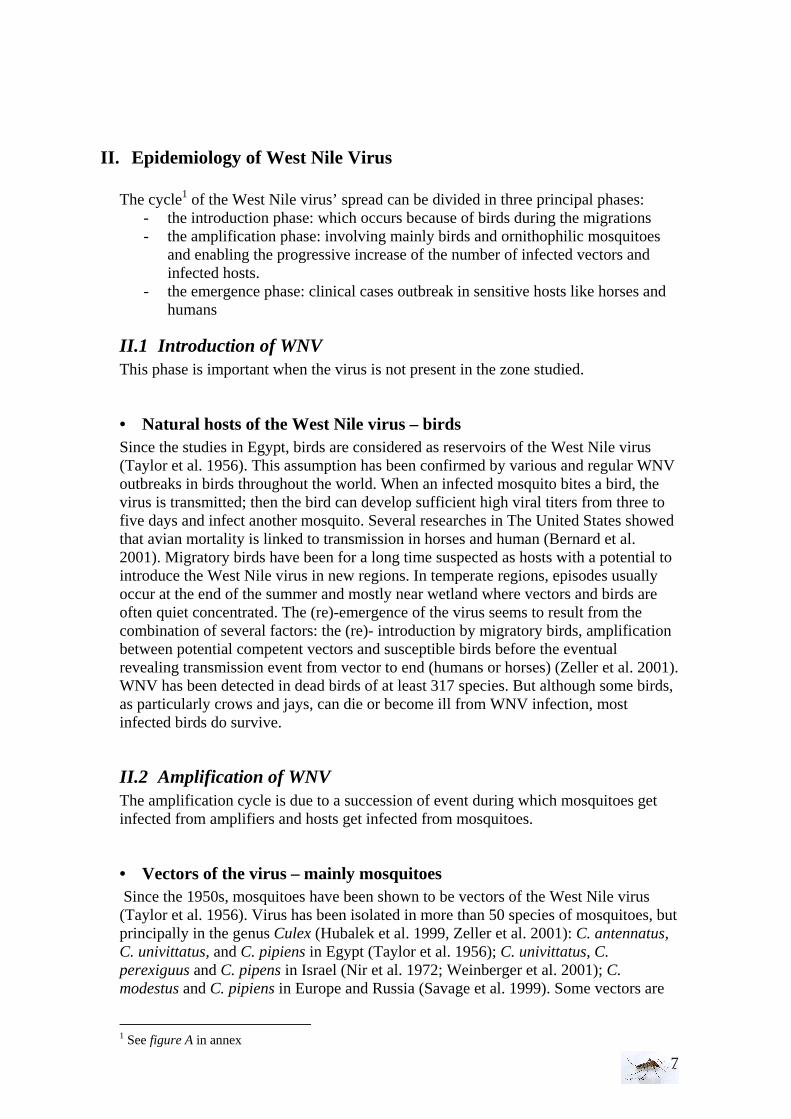
West Nile Virus has been officially discovered in the West Nile district of Uganda in 1937, isolated from a febrile adult woman (Smithburn et al. 1940). In the 1950s, the ecology of WNV has been characterized in Egypt by the researcher R. Taylor and his team. Their research enabled to identify the clues of the virus epidemiology and to establish the transmission cycles of the West Nile virus. To study the importance of the virus in human, serological surveys have been done among the Nil. Those researches showed a seasonal character of the disease, and an isolation of the virus between June and September. Sero-prevalence increases with the age which is an indication of endemic situation (Taylor et al. 1956). The virus turned out to be a cause of severe human meningoencephalitis (inflammation of the spinal cord and brain) in elderly patients during an outbreak in Israel in 1957 (Spigland et al. 1958). In the early 1960s, severe encephalitis were noted on human and also, for the first time in horses in France (Panthier 1968) and in Egypt. Serological surveys have also been done in birds and domestic animals to search for the presence of animal reservoirs. Thereby, the importance of the birds function in the transmission cycle and especially in the spread of the virus has been proved (Work et al. 1953). Concerning a potential vector role, among 80 000 arthropods inspected (acarid, flea, fly, louse, mosquito, tick), mosquitoes are the most enable to multiply the virus (Hurlbut 1956). Culex has been found to be the principal vector, transmitting the virus by bite after infection on viremic animal, notably, C. antennatus, C. pipiens Linnaeus, and C. univittatus in the Nile District. From 1994, much WNV encephalitis occurred in Europe and in the Mediterranean Basin (Murgue et al. 2001a, Dauphin et al. 2004), see table 1 in annexes. In 1999, the introduction of the virus in the United States changed the perception of the virus from a limited to a serious threat for human health. The strain of this West Nile virus episode, alike the isolated Israeli strain in 1998, seems to be introduced from the Near East (Lanciotti et al. 1999). Thereafter, West Nile virus spread throughout the American country (from the North of Canada in 2002 to Latin American countries).

1962-1965, 2000, 2003, 2004, 2006

1998

Figure 1: Recent WNV outbreaks in Western Europe

7

II. Epidemiology of West Nile Virus The cycle1 of the West Nile virus’ spread can be divided in three principal phases:

- the introduction phase: which occurs because of birds during the migrations - the amplification phase: involving mainly birds and ornithophilic mosquitoes

and enabling the progressive increase of the number of infected vectors and infected hosts.

- the emergence phase: clinical cases outbreak in sensitive hosts like horses and humans

II.1 Introduction of WNV This phase is important when the virus is not present in the zone studied.

• Natural hosts of the West Nile virus – birds Since the studies in Egypt, birds are considered as reservoirs of the West Nile virus (Taylor et al. 1956). This assumption has been confirmed by various and regular WNV outbreaks in birds throughout the world. When an infected mosquito bites a bird, the virus is transmitted; then the bird can develop sufficient high viral titers from three to five days and infect another mosquito. Several researches in The United States showed that avian mortality is linked to transmission in horses and human (Bernard et al. 2001). Migratory birds have been for a long time suspected as hosts with a potential to introduce the West Nile virus in new regions. In temperate regions, episodes usually occur at the end of the summer and mostly near wetland where vectors and birds are often quiet concentrated. The (re)-emergence of the virus seems to result from the combination of several factors: the (re)- introduction by migratory birds, amplification between potential competent vectors and susceptible birds before the eventual revealing transmission event from vector to end (humans or horses) (Zeller et al. 2001). WNV has been detected in dead birds of at least 317 species. But although some birds, as particularly crows and jays, can die or become ill from WNV infection, most infected birds do survive.

II.2 Amplification of WNV The amplification cycle is due to a succession of event during which mosquitoes get infected from amplifiers and hosts get infected from mosquitoes.

• Vectors of the virus – mainly mosquitoes Since the 1950s, mosquitoes have been shown to be vectors of the West Nile virus (Taylor et al. 1956). Virus has been isolated in more than 50 species of mosquitoes, but principally in the genus Culex (Hubalek et al. 1999, Zeller et al. 2001): C. antennatus, C. univittatus, and C. pipiens in Egypt (Taylor et al. 1956); C. univittatus, C. perexiguus and C. pipens in Israel (Nir et al. 1972; Weinberger et al. 2001); C. modestus and C. pipiens in Europe and Russia (Savage et al. 1999). Some vectors are

1 See figure A in annex

8

highly efficient as C. Tarsalis (Venkatesan et al. 2007) whereas others such as C. nigripalpus Theobald are moderately efficient (Turell et al. 2005). The vertical transmission has been demonstrated among certain species as C. pipiens (Dohm et al. 2002). The table 2 in annex presents the overview of potential WNV vectors in North West of Europe. To be involved as a vector, mosquito species have to satisfy specific requirements. The mosquitoes must have the capacity to become infected, to replicate and to transmit the virus with adequate hosts’ preference and with an activity during the period of virus circulation (Rogers et al. 2006, Balenghien 2006). To determine if the transmission cycle will be epizootic or enzootic, it is important to know the abundance of mosquitoes and their biting preference. Some species prefer to bite mammals (mammalophilic); others prefer birds (ornithophilic), whereas some vectors can be both, the so-called bridge vectors, who can transmit the WNV from birds to human and horses (e.g. C. pipiens, C. salinarius) (Gingrich et al. 2005). In Connecticut from June through October 1999-2003, West Nile virus has been isolated in Culex species (C. pipiens, C. salinarius, C. restuans), but also in Culiseta melanura and Aedes vexans, a mammalophilic species (Andreadis et al. 2004). Some studies showed, moreover, that the tick is a vector (Lawrie et al. 2004). Indeed, West Nile virus has also been isolated from soft (argasid) and hard (ixodid) tick species in regions of Europe, Africa, and Asia where WNV is endemic. Ticks have the second rank only after mosquitoes in their importance as vectors of human pathogens and transmit a greater variety of infectious agents than any other arthropod group (Lawrie et al. 2004).

• Transmission to the hosts – (mammals and humans) In the zones where most of the vectors are ornithophilic, we can wonder how the virus can be transmitted from birds to dead-end hosts (horses and human). Then, opportunists mosquitoes or no-purely mammalophilic can be sufficiently competent for the West Nile virus (=bridge vectors) or, Culex can also be not strictly ornithophilic (Balenghien 2006). The study of the trophic preference is crucial to understand how the ornithophilic Culex can spread the WNV to mammals. For examples, the blood meal of C. pipiens can characterize it as opportunist (Gingrich et al. 2005) or as ornithophilic (Molaei et al. 2006). Trophic preferences can be related to the genetic determinism. The Culex pipiens molestus is considered as autogenous, anthropophilic, and stenogamy whereas the Culex pipiens pipiens is defined as ornithophilic, eurygamy, and anautogenous (Kent et al. 2007). In experimental conditions, it has been showed that C. pipiens can transmit the virus from infected frog to healthy one (Rana ridibunda ) and to mice from 1 to 2 years old. Thus, frogs can be a natural reservoir of the virus (Kostyukov et al. 1986 and Vinogradova 2000). Through December 2001, CDC has also received a small number of reports of WN virus infection in bats, a skunk, a squirrel, a chipmunk, and a domestic rabbit. To be able to persist, a virus needs a combination of host(s) and vector(s) for which the reproduction ratio is above one. This combination is the core group for the virus. Other host(s) may become infected involving maybe also other vector(s) which is the satellite group in the infection dynamics. Of course, satellite groups can be very important to us when the satellite hosts are either humans or species important to humans (horses).

III. Risk infection model for the West Nile virus

9

The West Nile virus transmission involves, at least, a triptych interaction host-vector-pathogen. The term of host contains amplifier hosts (avian amplifiers) or core hosts and incidental or dead-end hosts (horses and humans) or satellite hosts. The risk of persistence should be estimated for the core hosts and from that a risk of infection follows for the incidental satellite hosts. In order to distinguish the main biological parameters involve in the West Nile virus transmission, the key parameters should be defined and estimated. The vectors density in space and time is one of those parameters.

• Transmission and vectorial capacity For an effective transmission, the pathogen should be present in a vertebrate blood during its biological cycle; a hematophage arthropod should have a sufficient ecologic contact with an amplifier host and the pathogen need to complete his development in the arthropod until infecting it. The transmission is possible if there is an encounter between the vectors and the pathogen presents in the amplifier host. Nevertheless, the transmission can be quite heterogeneous due to: diverse trophic behavior, different ecologic preferences. Then, undoubtedly, the environmental factors are important for the vectorial transmission and influence the vectorial competency and the vector density that is relevant for transmission. The quantification of the transmission rate in time and space rests on the identification of contacts between the different actors and the transmission probability upon contact. Thus, to analyze potential transmission rates, the possibility for persistence and the risks for satellite hosts, a model for the transmission has to be built. The purpose is to simplify the reality but to keep to relevant mechanism and identify the fundamental key parameters. Epidemic models help to obtain important practical insights into the epidemiology of infectious diseases. Epidemic theory has been instrumental to understand the threshold phenomena that govern the spread of infectious diseases. Ronald Ross (1910) discovered the malaria parasite in the gastrointestinal tract of the Anopheles mosquito, which led to the realization that malaria was transmitted by Anopheles, and laid the foundation for combating the disease. He showed that the number of mosquitoes per head of population must exceed a certain value for malaria to become endemic. This phenomenon finds formal expression in the threshold theorems derived from stochastic (Whittle 1955) and from deterministic (Kermack et al. 1927) epidemic models. Macdonald (1952) linked the entomologic aspects with the mathematical aspects. He studied the malaria, extended his basic models pioneered by Ross and defined the basic reproduction ratio R0, as a number of infections in a community directly linked to a unique immune case (Macdonald 1952). It is roughly equivalent to the number of animals that become infected through contact with one infectious individual. (6)

Let’s be:

- m the density of mosquitoes (Anopheles for the case of malaria) for a man, - a the biting rate of a female mosquito per day, - b the proportion of mosquitoes with infecting sporozoites in salivary gland = “

vectorial competency” - p the daily survival probability of mosquitoes - n the duration of the extrinsic incubation period in days, which refers to the

time between an infectious blood meal and infectiousness

pr

pbamaR

n

ln

...0 −

=

10

- 1/r the number of parasitemia days in a man= duration of infectious period for mosquitoes

- -1/ln p the mosquitoes’ life expectancy Then, a diseased will infect m.a Anopheles during 1/r parasitemia days, of which pn

will survive to the extrinsic incubation period and a fraction b of these will be infectious. The expression of R0 (6) can easily be modified and adapted for the WNV transmission by replacing men by birds. (ma.a.pn)/(-ln p) is the vectorial capacity. The lower the host density and thus the larger m the more blood meals will therefore be taken on a particular host.

When R0 >1, each human case will infect more than one human, then the disease will spread through the population and can persist. When R0<1, the disease will fade away eventually, and can not be at the origin of an epidemic in the population. Therefore, R0 is determinant for the epidemiological characterization of a transmission system, as well as the vectorial capacity formulated under the classical form (Garrett-Jones, 1964): (7) Then, the vectorial capacity corresponds to the product of the relative vectors’ density per host, by the proportion of vectors biting an host (due to the trophic preferences and inter-meal interval), by the infecting vectors percentage (which survived to the extrinsic incubation period) and by the number of infecting bites that vectors can inflict on the hosts’ population during the rest of their life (Tran et al. 2005). In enzootic WNV cycles, C. pipiens can be involved as main vector in dry areas and a secondary vector in wet areas. This mosquito is also the most abundant species collected engorged on horses in the dry areas. Then, C. pipiens can be considered as the principal WNV epidemic vector in the dry areas (Balenghien et al. 2006). The longevity, which gives the infectious average life and the population size, is one of the major factors to determine the transmission of vectors.

A POTENTIAL VECTOR

• Presentation of the Culex pipiens pipiens

Culex pipiens pipiens is one of the most widely distributed mosquito in the world, and moreover one of the most common in The Netherlands. It occurs on every continent except Antarctica and it is able to spread a number of diseases, especially arboviruses. Female has a short palpi and a blunt abdomen. Eggs are laid usually in rafts and the female can lay six to seven times in her lifespan (forty to fifty days). Culex pipiens pipiens prefers water contaminated with organic matter for the development of the larvae but is extremely adaptive to environmental conditions and the larvae are able to growth in a large variety of habitats (Vinogradova 2000).

• Sources for adult feeding and host seeking behavior Disease is spread only by females, because males do not bite. The blood meals are used to support the eggs’ development. Culex pipiens is described as zoophagic

p

pamC

n

ln

2

−××=

11

because it takes its meals from animals as well as humans and can also be described as ornithophagic because it frequently feeds on birds. Culex pipiens pipiens can therefore become a good vector and the disease can be difficult to eradicate because reservoir, such as birds, can spread the disease through a large area. C. p.p. has a peak activity at dusk and dawn.

A blood meal takes 2-7 days to digest and 1-3 meals are needed to complete development of clutch of eggs. The source and size of blood meal on fecundity and egg maturation have an importance for the gonotrophic relations. Indeed, there is a relation between blood weight and female weight about 2:1, when the female C. pipiens pipiens take a full blood meal (Vinogradova 2000). Transmission comes from repeated biting when the mosquito injects saliva that acts as an anticoagulant.

To elaborate the dynamic of the Culex pipiens pipiens, we want to study the development of larvae into adults and how possibility for development of larvae influences adult density. In particular the temperature effect on the development and adult emergence rates was studied.

Research questions To answer to these objectives, here are different questions to help to answer the two main research questions: Main research questions: QVE

1. What are the most important parameters that determine transmission of WNV and the risk of infection in transient host?

2. Where and during which period in the year can transmission of WNV be expected?

ENT

1. How is the dynamic population of Culex pipiens pipiens in The Netherlands under natural conditions in 3 different habitats?

2. What is the Life-table strategy of Culex pipiens? Sub-questions:

- What species of mosquitoes and birds transmit WN virus? - What are the different parameters which can influence the WNV (re)-emergence in North West of Europe? (Climatic data, reservoirs density, vectors density, dead-end hosts density, geographic situation, vegetation cover) - Which birds are reservoirs depending on the area in North West Europe? Corvids,

passerines, wild birds (amplifiers)? - What are the densities of mosquito and bird species that play a role in WN

amplification and transmission? - What is the Reproductive Number R0 that determines the dynamics of WNV

infection according to a special bird species? - Is the simple model well adapted to the NW Europe situation? - Is the R0 the same for the next generation? - What can be critical in the existing WNvirus model? - What can be improved?

12

SECOND PART:

MATERIEL AND METHODS

13

EPIDEMIOLOGY

WHICH MODEL TO USE AS A STARTING POINT FOR THE MODELLING OF WNV IN THE NORTH-WEST OF EUROPE?

Mathematical models are often successful in investigating the dynamics and possibility of control of an infectious disease. The transmission term is really important to predict the basic reproduction ratio R0 and depending how we choose the parameters, R0 can differ and thus the outbreak dynamic and the control decisions will be predicted differently. Wonham J. et al. (2006) reviewed seven arboviral models which share a standard structure for host and vector (susceptible-infectious- S-I). Among those seven models, three forms have been defined: the reservoir frequency dependence, the mass action, and the susceptible frequency dependence. This article shows how complex and subjective the building of a mathematical model can be. Disease transmission (between vectors and reservoirs) depends mostly on the mosquito biting rate “a”. Natural biting rates can also, vary by host density and mosquito species which could have a significant impact on virus transmission dynamics. Here, for this study we choose the mosquito Culex pipiens pipiens; nevertheless, still few data have been found about this mosquito in Europe. So, we have to make assumptions, using the existing models in adapting them as much as possible to our situation (particular vector, particular reservoir, and particular geographic area).

I. Building a WNV model suitable for the North West of Europe

I.1 What about the existing WNV models? • West Nile virus model of Thomas and Urena (2001) : Mass action form This model is a discrete-time model (time step of one week) which includes compartments for susceptible- exposed- infectious vectors, susceptible- infectious- recovered hosts (birds) and susceptible- infectious - recovered humans. They assume a vertical WNV transmission in the vector, then they introduce a proportion of infected mosquito births and classified them as exposed compartment. Moreover they assume that no birds die from WNV (just by natural death). They didn’t study the horses and omitted the human death. This model doesn’t make any difference between the transmission rates (vector to reservoir, reservoir to vector) and equal it to 1, which does not seem to be correct, because it has been proved that the number of bites per unit time by an individual vector, and the number of bites per unit time on an individual reservoir are different (Wonham et al. 2006). Moreover, Thomas and Urena model (2001) predicted that a reduction in bird density would help to

How could mathematical modelling help to understand West Nile virus dynamics in the North West of Europe?

Several WN virus model exist as Wonham and al. (2004) model, Bowman and al. (2005) model, Balenghien (2006) model, but no model has been made until

now for the North West of Europe. The purposes are, then, to study the existing models and find how accurate they are; to answer to the questions: can models be used to study West Nile virus outbreaks in the Netherlands? And finally, if yes what are the most important parameters to determine the risk infection?

14

control the epidemic, suggesting that the vector-to-reservoir transmission rate is a function of reservoir density. This theory has been criticized by Wonham et al. (2004) who showed that when reducing the reservoir density, it increased the R0 and then increase the probability to get an outbreak. • West Nile virus model of Lord & Day (2001): reservoir frequency dependence form This model consider the age structure of the reservoir, assuming that the juvenile birds are more susceptible to WNV and natural death than the adults, and certainly recover less rapidly from the infection. • West Nile virus model of Wonham et al. (2004): reservoir frequency dependence form Contrary to the Thomas and Urena (2001) model, Wonham et al. (2004) model studies the time as a continuous variable and it has a system of eight dimensional differential equations for vector and reservoir compartments. This model assumed virus induced death of birds but does not assume vertical transmission from mosquito adult to offspring. The cross-infection between mosquitoes and birds is modelled by mass action incidence and normalized by the total population of birds. Wonham et al. (2004) predicts that a reduction in bird density will intensify the WN virus outbreak rather than control, whereas a reduction of the mosquitoes’ density can be used to control the WNV outbreak. In reducing the reservoir density, it induced more frequently bites; then, it is more likely to find a infected reservoir and re-infected vectors. • West Nile virus model of Balenghien (2006) Balenghien T. defined the infection risk and made a model to predict the distribution of vector in space and time in the South of France. To estimate the WNV risk, he studied the vectorial competence, the contact between hosts and vectors and the dynamics of the number of mosquitoes in space and time. He showed that the transmission is dependent of the frequency of bites, the number of vector per host, the vectorial competence, the vector survival, and also the host viremia period. Thomas Balenghien introduced also the notion of dilution factor which is the proportion of blood filled vectors on others hosts than those considered. He divided the risk in two parts: the risk of getting infected vectors due to viremic bird and the risk of infection spread by infecting vectors. The study showed that Culex pipiens could participate to the enzootic transmission’s cycle where the density of vector and bird are sufficient, and showed also that C. pipiens bites mammal with a blood filled meal rate which seems to increase with temperature.

I.2 Can those models be used to predict WNV outbreaks in North-West Europe?

Based mainly on Lord & Day model (2001), Balenghien model (2006) and Wonham model (2004), a mathematical model to predict WNV outbreak in North-West Europe can indeed be proposed. The larval stage for the vector and the age structure of the reservoir are considered as important parameters to include in the model, but to simplify the model, we choose not to include them. Other parameters could have been also interesting to add, but would also have made the model too complex. Darbro & Harrington (2007) studied the influences of avian defensive behavior against host-seeking arthropods in the transmission of West Nile virus, which is the most detailed study of mosquito behavior in a single avian species. They exposed, in a large cage during the night, chickens (Gallus gallus domesticus L.) and house sparrows (Passer domesticus L.) to Culex pipiens pipiens L. and recorded for 6 hours. The author has determinate the mosquito blood-seeking success and the avian defensive behavior

15

rates. It has been found that both bird species showed a range of defensive behavior, and that the total behavior rates increased proportionally with mosquito density. The mosquito blood-feeding success was higher on house sparrows (82 +/- 5% and independent of behavior rates) than on chicken (58 +/- 5% and negatively correlated with defensive behavior rate after 1 hour of mosquito exposure). Moreover, both bird species did eat an average of 9.4 +/- 1.2% of mosquitoes, positively correlated with the defensive behavior. This article suggests that depending on the avian species, the anti-mosquito behavior changes, and then, can influence the blood-feeding success of mosquito. This difference might be due to the variability of the biting persistence on birds (Lord & Day, 2001), which can differ through mosquito species, tolerance or acceptance threshold of bites, and age structure of bird population. We understand that many variables and parameters enter into account to do a WNV model, but the aim is to make one as much as precise and simple as much as possible. Then, it is important to select the most useful parameters.

I.3 What are the most important parameters to determine WNV transmission and risks for dead-end hosts?

The SEIR model for the WNV in the Netherlands appears to be the most appropriate. It has been essential to identify the most important parameters to build a simple model, and the experiments in field and laboratory considerably helped to improve it. We know that the WNV cycle includes amplificatory host (-reservoir host - birds), vectors (mosquitoes), and dead-end hosts (especially horses and humans). Nevertheless, even if the infection may be significant for human, we consider that this last stage won’t affect the WNV dynamics. Then, the simplest model has been build with differential equations for vectors and reservoir host. The mosquito species studied is the most prevalent one in The Netherlands that is potentially able to spread the virus: Culex pipiens pipiens. Its lifecycle is around one month; thus, because we want to study one summer season the mosquito’s mortality and birth rate have been taken in account as parameters. The interesting birds for this study are mainly, wild duck, house crow (Corvus splendens), wood pigeon (Colomba palumbus), grey heron (Ardea cinerea), house sparrow (Passer domesticus) and Eurasian tree sparrow (Passer montanus). The model has been limited to the period from the end of June till the end of October. So, concerning the bird lifecycle, birth and mortality rates can be omitted. Nevertheless, question remains whether or not the juvenile stage has to be taken in account, as Lord & Day (2001) did? Indeed, if newborns are more susceptible to be bitten by mosquitoes than adult because they are less active or less defensive, then it would be interesting to take in account separate juvenile and adult birds’ stages. But we don’t know in Europe the biting rate of C. pipiens pipiens on juvenile and adult birds. So at first in our model we won’t take in account the age structure of bird populations. The most important parameters to determine the WNV risks are mostly the transmission rates (bird to mosquito, mosquito to host), the density of vector, the density of birds, the mortality rate, the larval density, the larval development time, the pupae development time, the mosquitos’ emergence. Some parameters will be taken from the literature and some will be determined with laboratory experiments. Among others, the concepts of vectors’ density and birds’ density are a bit complex. Indeed, the vectors density is defined as the number of female Culex pipiens pipiens catch in the Magnet liberty plus trap covering about 4000m2.

Nevertheless, this number correspond of three days of catching, whereas the density of birds is the number of birds (house sparrow) observed at time t during 5 min (on Tuesday and Friday) on 200m*200m. So, in the differential equations, the density of vectors will be calculated on the same area (40 000 m2). The notion of time is not the same in both cases. One

16

is a continuous observation (density of vectors “cumulated” over three days) and the other is a descriptive one each from a short observation. So to simplify the model, we choose to give both parameters at t time, and observe what happens during the 16 weeks of observation.

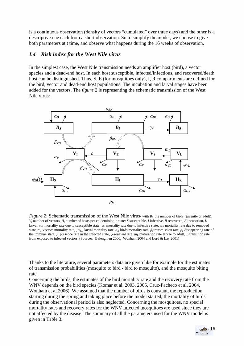
I.4 Risk index for the West Nile virus In the simplest case, the West Nile transmission needs an amplifier host (bird), a vector species and a dead-end host. In each host susceptible, infected/infectious, and recovered/death host can be distinguished. Thus, S, E (for mosquitoes only), I, R compartments are defined for the bird, vector and dead-end host populations. The incubation and larval stages have been added for the vectors. The figure 2 is representing the schematic transmission of the West Nile virus:

Figure 2: Schematic transmission of the West Nile virus- with Bi: the number of birds (juvenile or adult), Vi number of vectors, Hi number of hosts per epidemiologic state: S susceptible, I infective, R recovered, E incubation, L larval. αiS mortality rate due to susceptible state, αiI mortality rate due to infective state, αiR mortality rate due to removed state, αV vectors mortality rate, , αVL larval mortality rate, αB birds mortality rate, βi transmission rate, ρi disappearing rate of the immune state, γi presence rate in the infected state, φi renewal rate, mL maturation rate larvae to adult, ρ transition rate from exposed to infected vectors. (Sources: Balenghien 2006, Wonham 2004 and Lord & Lay 2001) Thanks to the literature, several parameters data are given like for example for the estimates of transmission probabilities (mosquito to bird - bird to mosquito), and the mosquito biting rate. Concerning the birds, the estimates of the bird mortality rate and the recovery rate from the WNV depends on the bird species (Komar et al. 2003, 2005, Cruz-Pacheco et al. 2004, Wonham et al.2006). We assumed that the number of birds is constant, the reproduction starting during the spring and taking place before the model started; the mortality of birds during the observational period is also neglected. Concerning the mosquitoes, no special mortality rates and recovery rates for the WNV infected mosquitoes are used since they are not affected by the disease. The summary of all the parameters used for the WNV model is given in Table 3.

αB

αVL

ρBN

γH

ρH

αHR αHI αHS

φH(t)

βVH αV αV

αV ρ

βVB

αB

γB

αBI αB

BS BI BR

VI VE VS

βBV

HS H I HR

VL mL

φVL

17

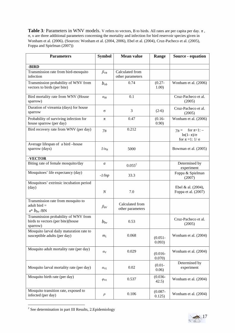
Table 3: Parameters in WNV models. V refers to vectors, B to birds. All rates are per capita per day. π , σ, υ are three additional parameters concerning the mortality and infection for bird reservoir species given in Wonham et al. (2006). (Sources: Wonham et al. (2004, 2006), Ebel et al. (2004), Cruz-Pacheco et al. (2005), Foppa and Spielman (2007))

Parameters Symbol Mean value Range Source - equation

-BIRD Transmission rate from bird-mosquito infection

βVB Calculated from other parameters

Transmission probability of WNV from vectors to birds (per bite)

bvb 0.74 (0.27-1.00)

Wonham et al. (2006)

Bird mortality rate from WNV (House sparrow)

αBI

0.1

Cruz-Pacheco et al. (2005)

Duration of vireamia (days) for house sparrow σ 3 (2-6)

Cruz-Pacheco et al. (2005)

Probability of surviving infection for house sparrow (per day)

π 0.47 (0.16-0.90)


Bird recovery rate from WNV (per day) γB

0.212

γB = for π<1: –ln(1- π)/σ

for π =1: 1/ σ Average lifespan of a bird –house sparrow (days)

1/αB 5000

Bowman et al. (2005)

-VECTOR Biting rate of female mosquito/day a

0.0552

Determined by experiment

Mosquitoes’ life expectancy (day) -1/lnp 33.3

Foppa & Spielman (2007)

Mosquitoes’ extrinsic incubation period (day)

N

7.0

Ebel & al. (2004), Foppa et al. (2007)

Transmission rate from mosquito to adult bird = a* bbv /BN

βBV

Calculated from other parameters

Transmission probability of WNV from birds to vectors (per bite)(house sparrow)

bbv 0.53 Cruz-Pacheco et al.

(2005)

Mosquito larval daily maturation rate to susceptible adults (per day) mL

0.068

(0.051-0.093)


Mosquito adult mortality rate (per day) αV

0.029

(0.016-0.070)


Mosquito larval mortality rate (per day)

αVL

0.02

(0.01-0.06)

Determined by experiment

Mosquito birth rate (per day)

φVL

0.537

(0.036-42.5)


Mosquito transition rate, exposed to infected (per day) ρ 0.106

(0.087-0.125)


2 See determination in part III Results, 2.Epidemiology

18

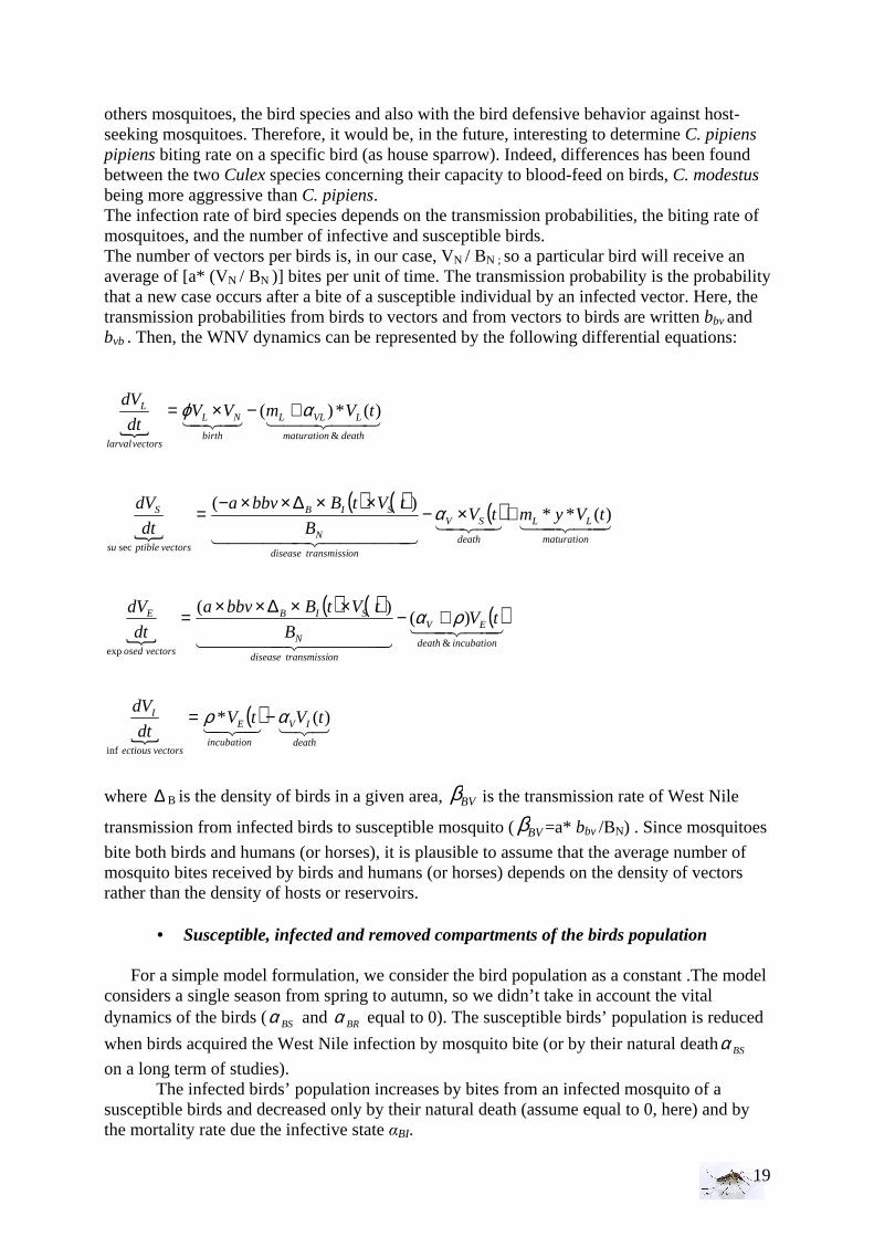
I.5 West Nile virus model formulation To describe the WNV dynamic in birds’ population and incidental hosts, the SIR system is used, whereas the SEI system is used for the vectors population (May et al. 1979). Each population is divided according to the epidemiologic state (susceptible S, in incubation E, infective I). Then, the population of birds is: BN = BS + BI + BR The population of female adult vectors is VN = VS + VE+ VI and VL the vector larvae (male and female). As it is difficult to distinguish female larvae from the male larvae, the sex ratio will be applied when the larvae pupate to study only the females thereafter. This is possible as the larvae do not contribute to the transmission anyway. Concerning the adult, we focus only on the female mosquitoes.

Finally, HN = HS + HI + HR

Below are presented the different equations to explain the evolution of the population according to the states (S, E, I, R) in function of the time:

• Larval stage, susceptible, incubation, and infected female mosquito’s stage

The susceptible female mosquito population size increases due to the immigration or birth susceptible mosquitoes at a constant rate φVL(t) . It is reduced when there is infection, which may happens when susceptible mosquito bites and feeds from the blood of infected birds, and by natural death due to their finite lifespan at a rate αVL.. It is considered that the incubation stage exists between the stages: susceptible and infected mosquitoes. The infected vector population appears because of the infection of susceptible mosquitoes by infected birds and diminishes by natural death αV. Moreover, it is assumed that the mosquitoes do not die from the West Nile virus and that the infected ones do not recover before their natural death. Last but not least, the vertical transmission in mosquitoes is supposed to be negligible, even if we know that WNV has been found in the north-eastern of United States where mosquitoes are inactive during the winter. Indeed, no documented studies have shown how WNV overwinters and reinitiates infection during the spring. Anderson et al. (2006) showed that WNV survives winter in unfed, vertically infected C. pipiens with amplification by horizontal transmission in spring. We considered a biting rate of female mosquito per day (“a”) and a sex ratio (”y”). The biting rate ‘’a’’ of mosquitoes is defined differently depending on the author, which make it important to include it correctly in the model. Some articles speak about the average number of bites per unit time by an individual vector, and others define it as the average number of bites per unit time on an individual reservoir. In addition, the biting rate can differ between juvenile host population and adult host population. Indeed, juveniles can be more disposed to be bitten than the adults because those latter can have more defensive behavior against the mosquito bites. Which means that the biting rate can differ depending on the bird (reservoir) age structure (biting rate on juvenile = aJ and biting rate on adult = aA). The proportion of blood meals taken on birds varies also seasonally (Edman, 1974).

After many considerations and due to a lack of data in Europe, we choose to take a fix biting rate for C. pipiens with the species house sparrow (Passer domesticus L.), the most common in the Netherlands. The host age structure was not studied here, because too complex in a short time of study. But we have to keep in mind that this biting rate is rather important and may change depending on the mosquito species, the mosquito density, the competition with

19

others mosquitoes, the bird species and also with the bird defensive behavior against host-seeking mosquitoes. Therefore, it would be, in the future, interesting to determine C. pipiens pipiens biting rate on a specific bird (as house sparrow). Indeed, differences has been found between the two Culex species concerning their capacity to blood-feed on birds, C. modestus being more aggressive than C. pipiens. The infection rate of bird species depends on the transmission probabilities, the biting rate of mosquitoes, and the number of infective and susceptible birds. The number of vectors per birds is, in our case, VN / BN ; so a particular bird will receive an average of [a* (VN / BN )] bites per unit of time. The transmission probability is the probability that a new case occurs after a bite of a susceptible individual by an infected vector. Here, the transmission probabilities from birds to vectors and from vectors to birds are written bbv and bvb . Then, the WNV dynamics can be represented by the following differential equations:

{

{

( ) ( ) ( )

{

( ) ( ) ( )

{( )

32143421

443442144444 344444 21

44344214342144444 344444 21

44 344 2143421

death

IV

incubation

E

vectorsectious

I

incubationdeath

EV

ontransmissidisease

N

SIB

vectorsosed

E

maturation

LL

death

SV

ontransmissidisease

N

SIB

vectorsptiblesu

S

deathmaturation

LVLL

birth

NL

vectorslarval

L

tVtVdt

dV

tVB

tVtBbbva

dt

dV

tVymtVB

tVtBbbva

dt

dV

tVmVVdt

dV

)(*

)()(

)(**)(

)(*)(

inf

&exp

sec

&

αρ

ρα

α

αϕ

−=

+−××∆××=

+×−××∆××−=

+−×=

where ∆ B is the density of birds in a given area, BVβ is the transmission rate of West Nile

transmission from infected birds to susceptible mosquito ( BVβ =a* bbv /BN) . Since mosquitoes

bite both birds and humans (or horses), it is plausible to assume that the average number of mosquito bites received by birds and humans (or horses) depends on the density of vectors rather than the density of hosts or reservoirs.

• Susceptible, infected and removed compartments of the birds population

For a simple model formulation, we consider the bird population as a constant .The model considers a single season from spring to autumn, so we didn’t take in account the vital dynamics of the birds (BSα and BRα equal to 0). The susceptible birds’ population is reduced

when birds acquired the West Nile infection by mosquito bite (or by their natural deathBSα

on a long term of studies). The infected birds’ population increases by bites from an infected mosquito of a susceptible birds and decreased only by their natural death (assume equal to 0, here) and by the mortality rate due the infective state αBI.

20

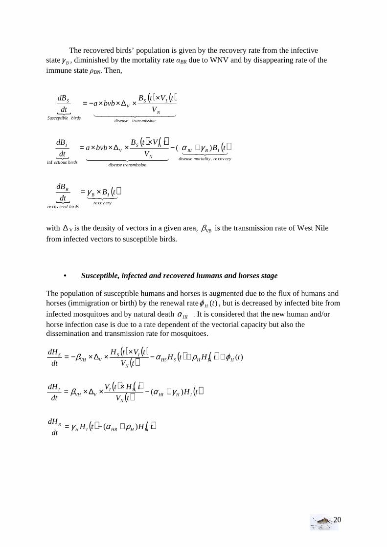
The recovered birds’ population is given by the recovery rate from the infective state Bγ , diminished by the mortality rate αBR due to WNV and by disappearing rate of the immune state ρBN. Then,

{

( ) ( )

{

( ) ( ) ( )

{( )

43421

44 344 214444 34444 21

4444 34444 21

eryre

IB

birdseredre

R

eryremortalitydisease

IBBI

ontransmissidisease

N

ISV

birdsectious

I

ontransmissidisease

N

ISV

birdseSusceptibl

S

tBdt

dB

tBV

tVtBbvba

dt

dB

V

tVtBbvba

dt

dB

covcov

cov,inf

)(

×=

+−×

×∆××=

××∆××−=

γ

γα

with ∆ V is the density of vectors in a given area, VBβ is the transmission rate of West Nile

from infected vectors to susceptible birds.

• Susceptible, infected and recovered humans and horses stage

The population of susceptible humans and horses is augmented due to the flux of humans and horses (immigration or birth) by the renewal rate )(tHϕ , but is decreased by infected bite from

infected mosquitoes and by natural death HIα . It is considered that the new human and/or horse infection case is due to a rate dependent of the vectorial capacity but also the dissemination and transmission rate for mosquitoes.

( ) ( )( ) ( ) ( )

( ) ( )( ) ( )

( ) ( )tHtHdt

dH

tHtV

tHtV

dt

dH

ttHtHtV

tVtH

dt

dH

RHHRIHR

IHHIN

SIVVH

I

HRHSHSN

ISVVH

S

)(

)(

)(

ραγ

γαβ

ϕραβ

+−=

+−××∆×=

++−××∆×−=

21

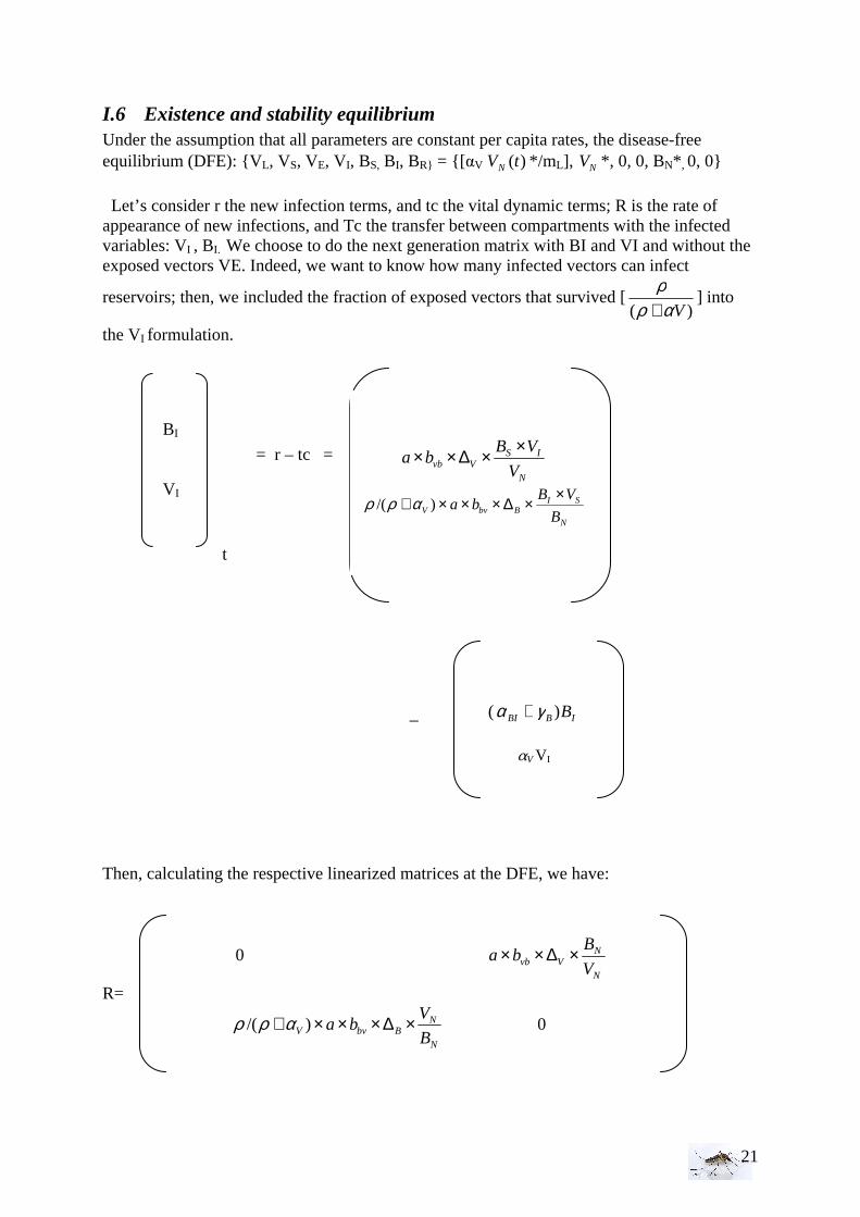
I.6 Existence and stability equilibrium Under the assumption that all parameters are constant per capita rates, the disease-free equilibrium (DFE): {VL, VS, VE, VI, BS, BI, BR} = {[αV )(tVN */mL], NV *, 0, 0, BN* , 0, 0}

Let’s consider r the new infection terms, and tc the vital dynamic terms; R is the rate of appearance of new infections, and Tc the transfer between compartments with the infected variables: VI , BI. We choose to do the next generation matrix with BI and VI and without the exposed vectors VE. Indeed, we want to know how many infected vectors can infect

reservoirs; then, we included the fraction of exposed vectors that survived [)( Vαρ

ρ+

] into

the VI formulation. = r – tc = t _ Then, calculating the respective linearized matrices at the DFE, we have: R=

BI VI

N

ISVvb V

VBba

××∆××

N

SIBbvV B

VBba

××∆×××+ )/( αρρ

( IBBI B)γα +

αV V I

0 N

NVvb V

Bba ×∆××

N

NBbvV B

Vba ×∆×××+ )/( αρρ 0

22

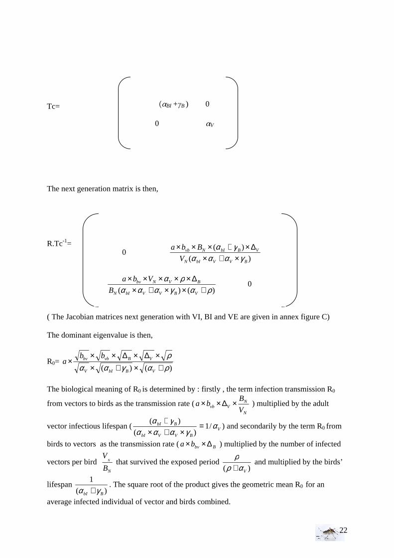
Tc= The next generation matrix is then, R.Tc-1=

( The Jacobian matrices next generation with VI, BI and VE are given in annex figure C) The dominant eigenvalue is then,

R0= )()( ραγαα

ρ+×+×

×∆×∆×××

VBbIV

VBvbbv bba

The biological meaning of R0 is determined by : firstly , the term infection transmission R0

from vectors to birds as the transmission rate (N

NVvb V

Bba ×∆×× ) multiplied by the adult

vector infectious lifespan ( VBVVbI

BbI αγααα

γα/1

)(

)( =×+×

+) and secondarily by the term R0 from

birds to vectors as the transmission rate ( Bbvba ∆×× ) multiplied by the number of infected

vectors per bird NB

VN that survived the exposed period

)( Vαρρ+

and multiplied by the birds’

lifespan )(

1

BbI γα +. The square root of the product gives the geometric mean R0 for an

average infected individual of vector and birds combined.

(αBI +γB ) 0 0 αV

0 )(

)(

BVVbIN

VBbINvb

V

Bba

γαααγα×+×

∆×+×××

)()( ραγααα

ρα+××+×

∆×××××

VBVVbIN

BVNbv

B

Vba 0

23

The model has to be a simple as possible despite the complexity of the WNV transmission. Now that the model is established, the question is: is the model

behaviour realistic and credible?

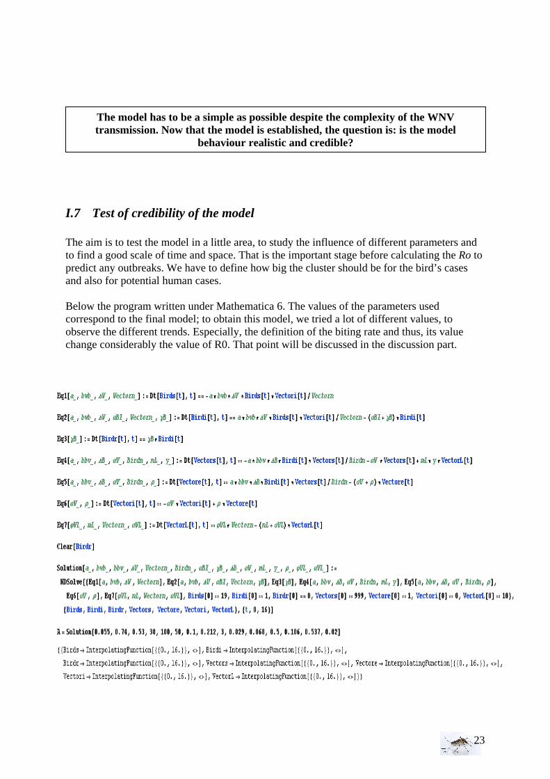
I.7 Test of credibility of the model The aim is to test the model in a little area, to study the influence of different parameters and to find a good scale of time and space. That is the important stage before calculating the Ro to predict any outbreaks. We have to define how big the cluster should be for the bird’s cases and also for potential human cases. Below the program written under Mathematica 6. The values of the parameters used correspond to the final model; to obtain this model, we tried a lot of different values, to observe the different trends. Especially, the definition of the biting rate and thus, its value change considerably the value of R0. That point will be discussed in the discussion part.

24

No.

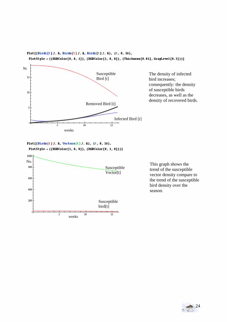
The density of infected bird increases; consequently: the density of susceptible birds decreases, as well as the density of recovered birds.

Susceptible Bird [t]

Removed Bird [t]

Infected Bird [t]

Susceptible bird[t]

This graph shows the trend of the susceptible vector density compare to the trend of the susceptible bird density over the season.

Susceptible Vector[t]

weeks

weeks

No.

25

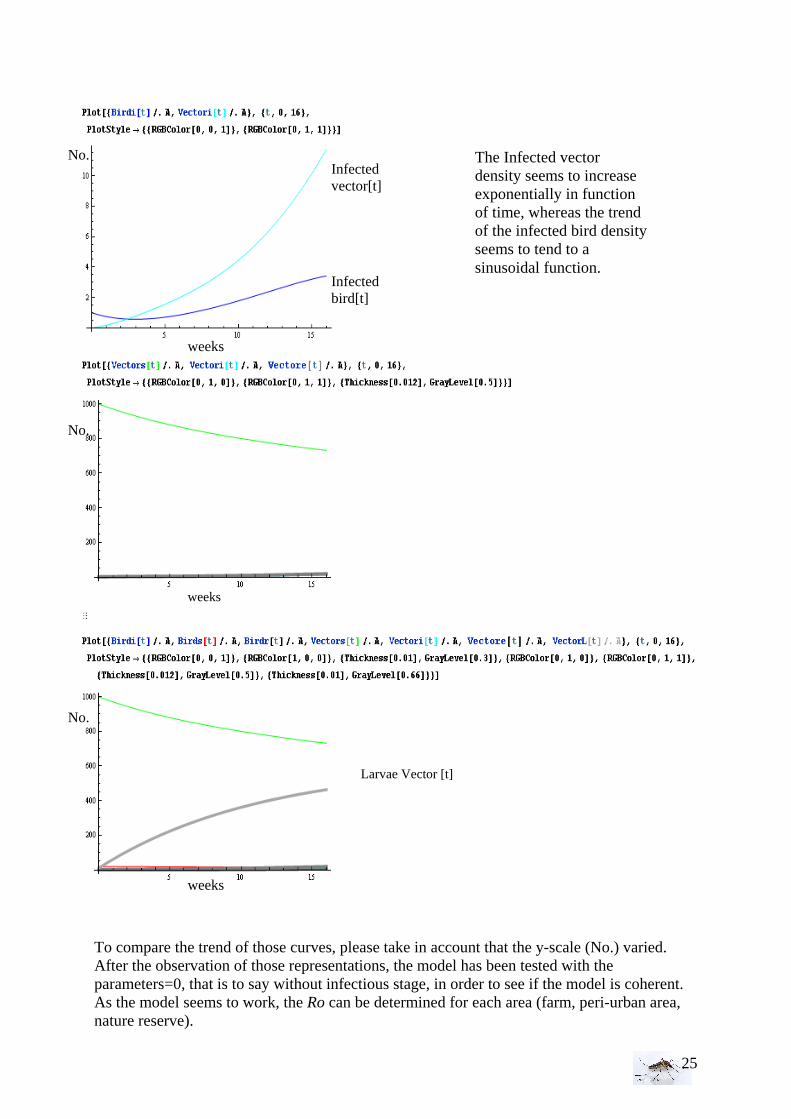
To compare the trend of those curves, please take in account that the y-scale (No.) varied. After the observation of those representations, the model has been tested with the parameters=0, that is to say without infectious stage, in order to see if the model is coherent. As the model seems to work, the Ro can be determined for each area (farm, peri-urban area, nature reserve).

The Infected vector density seems to increase exponentially in function of time, whereas the trend of the infected bird density seems to tend to a sinusoidal function.

Infected vector[t]

Infected bird[t]

weeks

weeks

weeks

No.

Larvae Vector [t]

No.

No.

26

ENTOMOLOGY

The ecology of Culex pipiens pipiens in The Netherlands

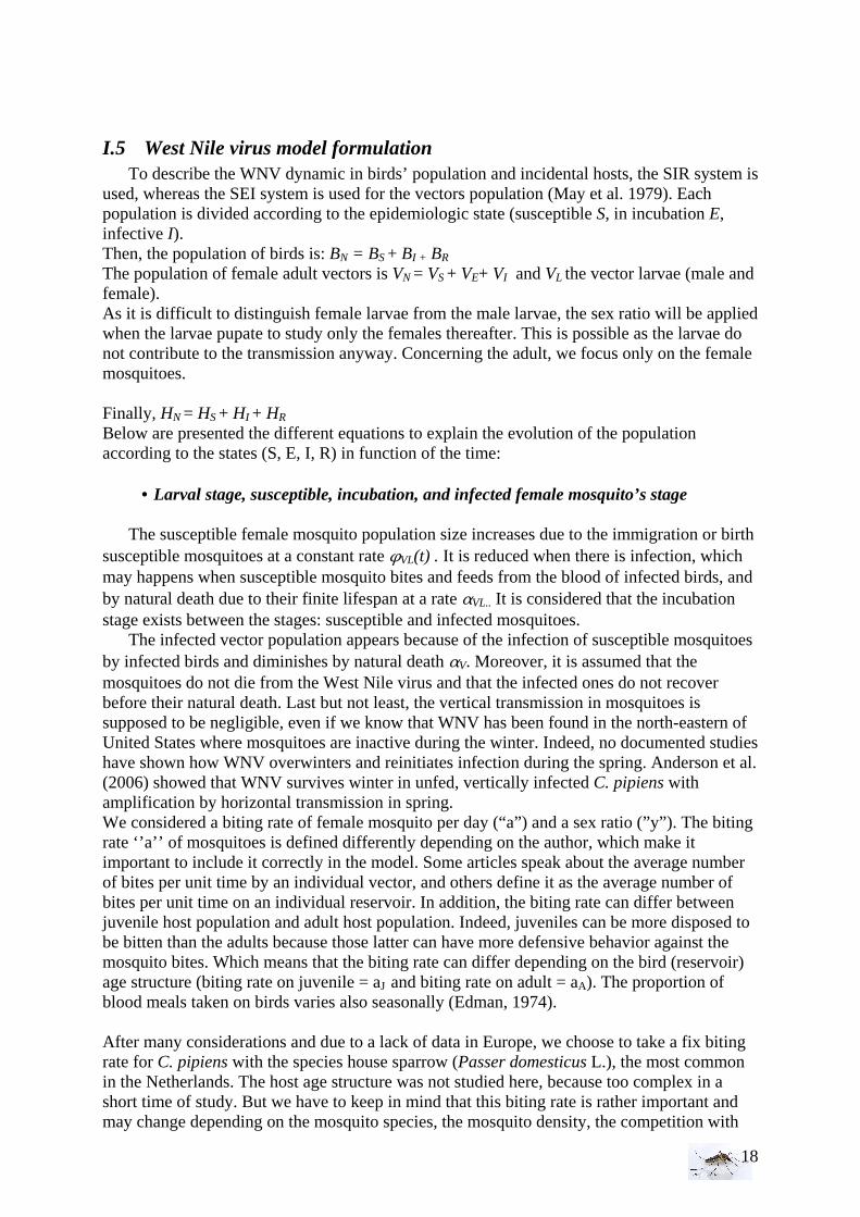
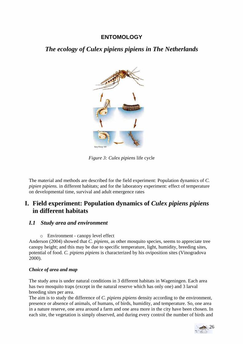
Figure 3: Culex pipiens life cycle

The material and methods are described for the field experiment: Population dynamics of C. pipien pipiens. in different habitats; and for the laboratory experiment: effect of temperature on developmental time, survival and adult emergence rates

I. Field experiment: Population dynamics of Culex pipiens pipiens in different habitats

I.1 Study area and environment

o Environment - canopy level effect Anderson (2004) showed that C. pipiens, as other mosquito species, seems to appreciate tree canopy height; and this may be due to specific temperature, light, humidity, breeding sites, potential of food. C. pipiens pipiens is characterized by his oviposition sites (Vinogradova 2000). Choice of area and map The study area is under natural conditions in 3 different habitats in Wageningen. Each area has two mosquito traps (except in the natural reserve which has only one) and 3 larval breeding sites per area. The aim is to study the difference of C. pipiens pipiens density according to the environment, presence or absence of animals, of humans, of birds, humidity, and temperature. So, one area in a nature reserve, one area around a farm and one area more in the city have been chosen. In each site, the vegetation is simply observed, and during every control the number of birds and

27

animals are noted in a periphery of approximately 200m (C. pipiens has a flight range of 1 to 3.5km, longer distance in hot day than in cooler weather). It is also known that C. pipiens prefers to breed in standing water, especially in water polluted with organic matter. The sampling sites have been determined based on the accessibility, availability and representativeness of the respective area.

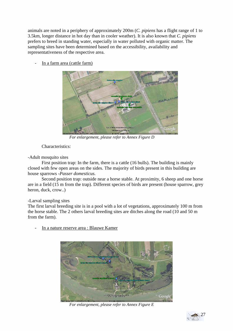
- In a farm area (cattle farm)

For enlargement, please refer to Annex Figure D

Characteristics:

-Adult mosquito sites First position trap: In the farm, there is a cattle (16 bulls). The building is mainly

closed with few open areas on the sides. The majority of birds present in this building are house sparrows -Passer domesticus.

Second position trap: outside near a horse stable. At proximity, 6 sheep and one horse are in a field (15 m from the trap). Different species of birds are present (house sparrow, grey heron, duck, crow..) -Larval sampling sites The first larval breeding site is in a pool with a lot of vegetations, approximately 100 m from the horse stable. The 2 others larval breeding sites are ditches along the road (10 and 50 m from the farm).

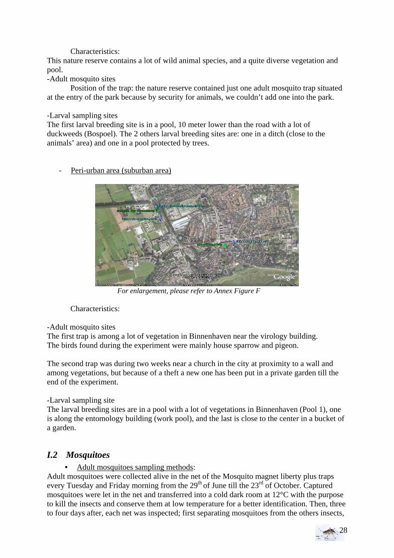
- In a nature reserve area : Blauwe Kamer

For enlargement, please refer to Annex Figure E

28

Characteristics: This nature reserve contains a lot of wild animal species, and a quite diverse vegetation and pool. -Adult mosquito sites

Position of the trap: the nature reserve contained just one adult mosquito trap situated at the entry of the park because by security for animals, we couldn’t add one into the park. -Larval sampling sites The first larval breeding site is in a pool, 10 meter lower than the road with a lot of duckweeds (Bospoel). The 2 others larval breeding sites are: one in a ditch (close to the animals’ area) and one in a pool protected by trees.

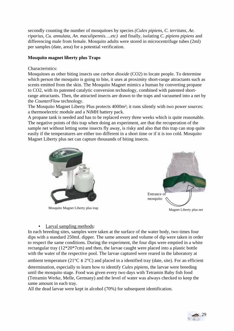
- Peri-urban area (suburban area)

For enlargement, please refer to Annex Figure F

Characteristics:

-Adult mosquito sites The first trap is among a lot of vegetation in Binnenhaven near the virology building. The birds found during the experiment were mainly house sparrow and pigeon. The second trap was during two weeks near a church in the city at proximity to a wall and among vegetations, but because of a theft a new one has been put in a private garden till the end of the experiment. -Larval sampling site The larval breeding sites are in a pool with a lot of vegetations in Binnenhaven (Pool 1), one is along the entomology building (work pool), and the last is close to the center in a bucket of a garden.

I.2 Mosquitoes • Adult mosquitoes sampling methods:

Adult mosquitoes were collected alive in the net of the Mosquito magnet liberty plus traps every Tuesday and Friday morning from the 29th of June till the 23rd of October. Captured mosquitoes were let in the net and transferred into a cold dark room at 12°C with the purpose to kill the insects and conserve them at low temperature for a better identification. Then, three to four days after, each net was inspected; first separating mosquitoes from the others insects,

29

secondly counting the number of mosquitoes by species (Culex pipiens, C. territans, Ae. riparius, Cu. annulata, An. maculipennis….etc) and finally, isolating C. pipiens pipiens and differencing male from female. Mosquito adults were stored in microcentrifuge tubes (2ml) per samples (date, area) for a potential verification. Mosquito magnet liberty plus Traps Characteristics: Mosquitoes as other biting insects use carbon dioxide (CO2) to locate people. To determine which person the mosquito is going to bite, it uses at proximity short-range attractants such as scents emitted from the skin. The Mosquito Magnet mimics a human by converting propane to CO2, with its patented catalytic conversion technology, combined with patented short-range attractants. Then, the attracted insects are drawn to the traps and vacuumed into a net by the CounterFlow technology. The Mosquito Magnet Liberty Plus protects 4000m²; it runs silently with two power sources: a thermoelectric module and a NiMH battery pack. A propane tank is needed and has to be replaced every three weeks which is quite reasonable. The negative points of this trap when doing an experiment, are that the recuperation of the sample net without letting some insects fly away, is risky and also that this trap can stop quite easily if the temperatures are either too different in a short time or if it is too cold. Mosquito Magnet Liberty plus net can capture thousands of biting insects.

• Larval sampling methods: In each breeding sites, samples were taken at the surface of the water body, two times four dips with a standard 250mL dipper. The same amount and volume of dip were taken in order to respect the same conditions. During the experiment, the four dips were emptied in a white rectangular tray (12*20*7cm) and then, the larvae caught were placed into a plastic bottle with the water of the respective pool. The larvae captured were reared in the laboratory at

ambient temperature (21°C ± 2°C) and placed in a identified tray (date, site). For an efficient

determination, especially to learn how to identify Culex pipiens, the larvae were breeding until the mosquito stage. Food was given every two days with Tetramin Baby fish food (Tetramin Werke, Melle, Germany) and the level of water was always checked to keep the same amount in each tray. All the dead larvae were kept in alcohol (70%) for subsequent identification.

Mosquito Magnet Liberty plus trap

Entrance of mosquito

Magnet Liberty plus net

30

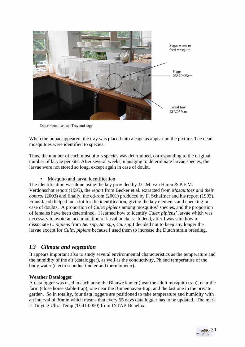
When the pupae appeared, the tray was placed into a cage as appear on the picture. The dead mosquitoes were identified to species. Thus, the number of each mosquito’s species was determined, corresponding to the original number of larvae per site. After several weeks, managing to determinate larvae species, the larvae were not stored so long, except again in case of doubt.

• Mosquito and larval identification The identification was done using the key provided by J.C.M. van Haren & P.F.M. Verdonschot report (1995), the report from Becker et al. extracted from Mosquitoes and their control (2003) and finally, the cd-rom (2001) produced by F. Schaffner and his report (1993). Frans Jacob helped me a lot for the identification, giving the key elements and checking in case of doubts. A proportion of Culex pipiens among mosquitos’ species, and the proportion of females have been determined. I learned how to identify Culex pipiens’ larvae which was necessary to avoid an accumulation of larval buckets. Indeed, after I was sure how to dissociate C. pipiens from Ae. spp, An. spp, Cu. spp,I decided not to keep any longer the larvae except for Culex pipiens because I used them to increase the Dutch strain breeding.

I.3 Climate and vegetation It appears important also to study several environmental characteristics as the temperature and the humidity of the air (datalogger), as well as the conductivity, Ph and temperature of the body water (electro-conductimeter and thermometer). Weather Datalogger A datalogger was used in each area: the Blauwe kamer (near the adult mosquito trap), near the farm (close horse stable-trap), one near the Binnenhaven-trap, and the last one in the private garden. So in totality, four data loggers are positioned to take temperature and humidity with an interval of 30min which means that every 55 days data logger has to be updated. The mark is Tinytag Ultra Temp (TGU-0050) from INTAB Benelux.

Sugar water to feed mosquito

Cage 25*25*25cm

Larval tray 12*20*7cm

Experimental set-up: Tray and cage

31

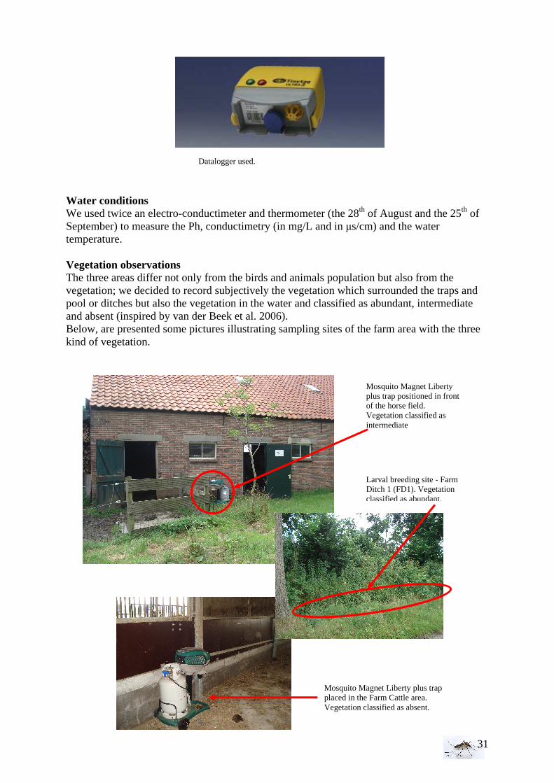
Water conditions We used twice an electro-conductimeter and thermometer (the 28th of August and the 25th of September) to measure the Ph, conductimetry (in mg/L and in µs/cm) and the water temperature. Vegetation observations The three areas differ not only from the birds and animals population but also from the vegetation; we decided to record subjectively the vegetation which surrounded the traps and pool or ditches but also the vegetation in the water and classified as abundant, intermediate and absent (inspired by van der Beek et al. 2006). Below, are presented some pictures illustrating sampling sites of the farm area with the three kind of vegetation.

Mosquito Magnet Liberty plus trap positioned in front of the horse field. Vegetation classified as intermediate

Larval breeding site - Farm Ditch 1 (FD1). Vegetation classified as abundant.

Mosquito Magnet Liberty plus trap placed in the Farm Cattle area. Vegetation classified as absent.

Datalogger used.

32

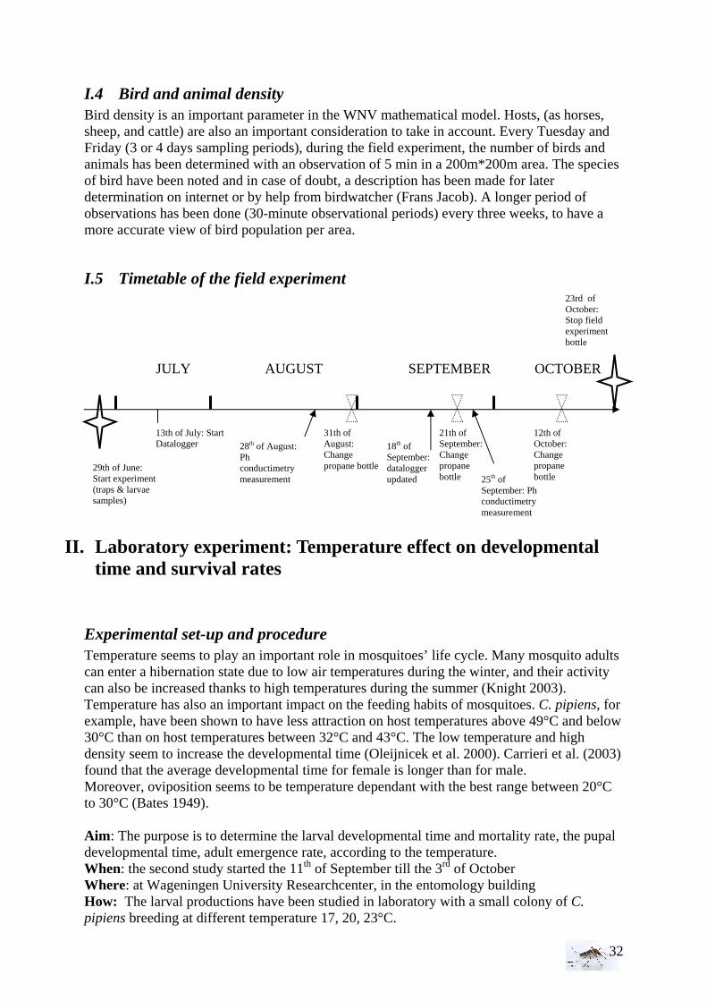
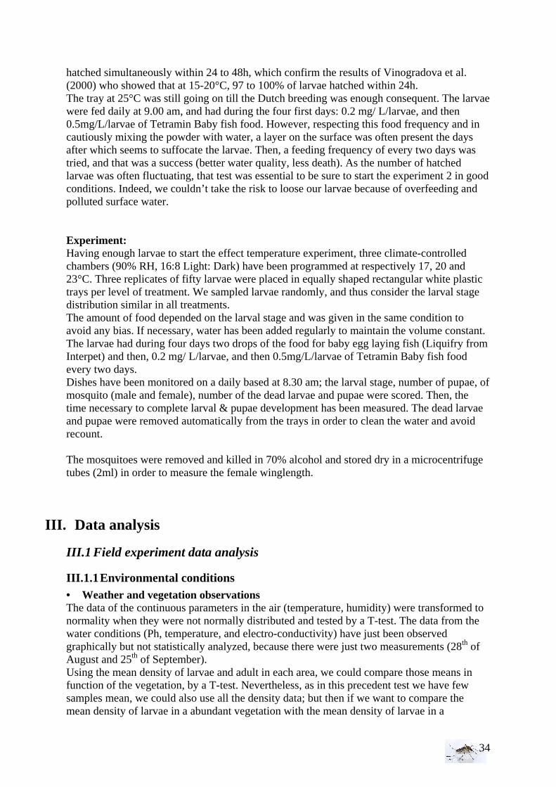
I.4 Bird and animal density Bird density is an important parameter in the WNV mathematical model. Hosts, (as horses, sheep, and cattle) are also an important consideration to take in account. Every Tuesday and Friday (3 or 4 days sampling periods), during the field experiment, the number of birds and animals has been determined with an observation of 5 min in a 200m*200m area. The species of bird have been noted and in case of doubt, a description has been made for later determination on internet or by help from birdwatcher (Frans Jacob). A longer period of observations has been done (30-minute observational periods) every three weeks, to have a more accurate view of bird population per area.

I.5 Timetable of the field experiment

II. Laboratory experiment: Temperature effect on developmental time and survival rates

Experimental set-up and procedure Temperature seems to play an important role in mosquitoes’ life cycle. Many mosquito adults can enter a hibernation state due to low air temperatures during the winter, and their activity can also be increased thanks to high temperatures during the summer (Knight 2003). Temperature has also an important impact on the feeding habits of mosquitoes. C. pipiens, for example, have been shown to have less attraction on host temperatures above 49°C and below 30°C than on host temperatures between 32°C and 43°C. The low temperature and high density seem to increase the developmental time (Oleijnicek et al. 2000). Carrieri et al. (2003) found that the average developmental time for female is longer than for male. Moreover, oviposition seems to be temperature dependant with the best range between 20°C to 30°C (Bates 1949). Aim : The purpose is to determine the larval developmental time and mortality rate, the pupal developmental time, adult emergence rate, according to the temperature. When: the second study started the 11th of September till the 3rd of October Where: at Wageningen University Researchcenter, in the entomology building How: The larval productions have been studied in laboratory with a small colony of C. pipiens breeding at different temperature 17, 20, 23°C.

25th of September: Ph conductimetry measurement

18th of September: datalogger updated

31th of August: Change propane bottle

21th of September: Change propane bottle

29th of June: Start experiment (traps & larvae samples)

13th of July: Start Datalogger

12th of October: Change propane bottle

23rd of October: Stop field experiment bottle

JULY AUGUST SEPTEMBER OCTOBER

28th of August: Ph conductimetry measurement

33

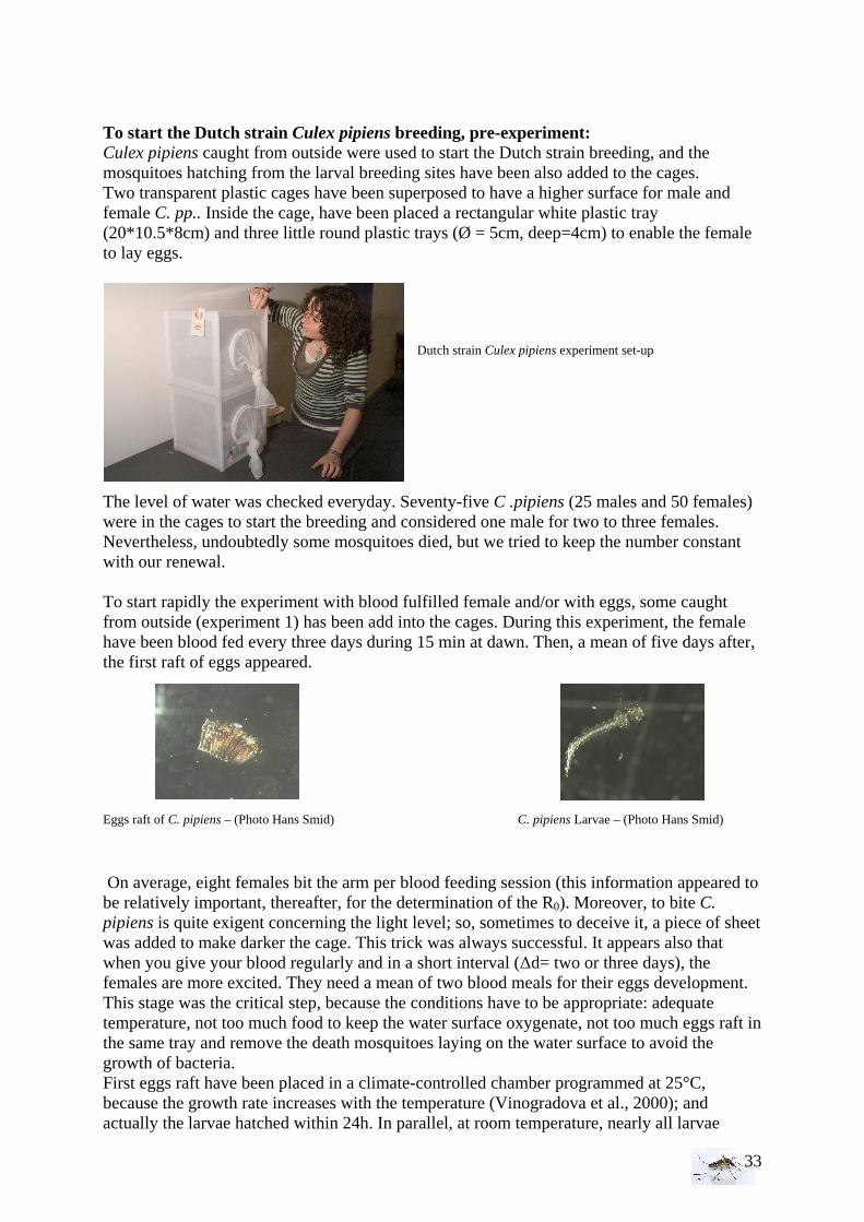
To start the Dutch strain Culex pipiens breeding, pre-experiment: Culex pipiens caught from outside were used to start the Dutch strain breeding, and the mosquitoes hatching from the larval breeding sites have been also added to the cages. Two transparent plastic cages have been superposed to have a higher surface for male and female C. pp.. Inside the cage, have been placed a rectangular white plastic tray (20*10.5*8cm) and three little round plastic trays (Ø = 5cm, deep=4cm) to enable the female to lay eggs.

Dutch strain Culex pipiens experiment set-up

The level of water was checked everyday. Seventy-five C .pipiens (25 males and 50 females) were in the cages to start the breeding and considered one male for two to three females. Nevertheless, undoubtedly some mosquitoes died, but we tried to keep the number constant with our renewal. To start rapidly the experiment with blood fulfilled female and/or with eggs, some caught from outside (experiment 1) has been add into the cages. During this experiment, the female have been blood fed every three days during 15 min at dawn. Then, a mean of five days after, the first raft of eggs appeared. Eggs raft of C. pipiens – (Photo Hans Smid) C. pipiens Larvae – (Photo Hans Smid)

On average, eight females bit the arm per blood feeding session (this information appeared to be relatively important, thereafter, for the determination of the R0). Moreover, to bite C. pipiens is quite exigent concerning the light level; so, sometimes to deceive it, a piece of sheet was added to make darker the cage. This trick was always successful. It appears also that when you give your blood regularly and in a short interval (∆d= two or three days), the females are more excited. They need a mean of two blood meals for their eggs development. This stage was the critical step, because the conditions have to be appropriate: adequate temperature, not too much food to keep the water surface oxygenate, not too much eggs raft in the same tray and remove the death mosquitoes laying on the water surface to avoid the growth of bacteria. First eggs raft have been placed in a climate-controlled chamber programmed at 25°C, because the growth rate increases with the temperature (Vinogradova et al., 2000); and actually the larvae hatched within 24h. In parallel, at room temperature, nearly all larvae

34

hatched simultaneously within 24 to 48h, which confirm the results of Vinogradova et al. (2000) who showed that at 15-20°C, 97 to 100% of larvae hatched within 24h. The tray at 25°C was still going on till the Dutch breeding was enough consequent. The larvae were fed daily at 9.00 am, and had during the four first days: 0.2 mg/ L/larvae, and then 0.5mg/L/larvae of Tetramin Baby fish food. However, respecting this food frequency and in cautiously mixing the powder with water, a layer on the surface was often present the days after which seems to suffocate the larvae. Then, a feeding frequency of every two days was tried, and that was a success (better water quality, less death). As the number of hatched larvae was often fluctuating, that test was essential to be sure to start the experiment 2 in good conditions. Indeed, we couldn’t take the risk to loose our larvae because of overfeeding and polluted surface water. Experiment: Having enough larvae to start the effect temperature experiment, three climate-controlled chambers (90% RH, 16:8 Light: Dark) have been programmed at respectively 17, 20 and 23°C. Three replicates of fifty larvae were placed in equally shaped rectangular white plastic trays per level of treatment. We sampled larvae randomly, and thus consider the larval stage distribution similar in all treatments. The amount of food depended on the larval stage and was given in the same condition to avoid any bias. If necessary, water has been added regularly to maintain the volume constant. The larvae had during four days two drops of the food for baby egg laying fish (Liquifry from Interpet) and then, 0.2 mg/ L/larvae, and then 0.5mg/L/larvae of Tetramin Baby fish food every two days. Dishes have been monitored on a daily based at 8.30 am; the larval stage, number of pupae, of mosquito (male and female), number of the dead larvae and pupae were scored. Then, the time necessary to complete larval & pupae development has been measured. The dead larvae and pupae were removed automatically from the trays in order to clean the water and avoid recount. The mosquitoes were removed and killed in 70% alcohol and stored dry in a microcentrifuge tubes (2ml) in order to measure the female winglength.

III. Data analysis

III.1 Field experiment data analysis

III.1.1 Environmental conditions • Weather and vegetation observations The data of the continuous parameters in the air (temperature, humidity) were transformed to normality when they were not normally distributed and tested by a T-test. The data from the water conditions (Ph, temperature, and electro-conductivity) have just been observed graphically but not statistically analyzed, because there were just two measurements (28th of August and 25th of September). Using the mean density of larvae and adult in each area, we could compare those means in function of the vegetation, by a T-test. Nevertheless, as in this precedent test we have few samples mean, we could also use all the density data; but then if we want to compare the mean density of larvae in a abundant vegetation with the mean density of larvae in a

35

intermediate vegetation, it appears that we have twice more sites with abundant vegetation which make the samples unequal. • Bird and animal density With the Kruskall-Wallis test, the equality of populations rank test has been studied for animals and then birds between the area (1=RN, 2= FC, 3= FH, 4=PUB, 5=PUC). As for the statistical analysis of the larval density, if H0 is rejected then we proceed to a Wilcoxon rank-sum test, more precise comparing two by two areas.

III.1.2 Mosquito collection per area As we scored the density of mosquitoes caught in the traps every 3 or 4 days, we can first observe the mosquito distribution per site and then decide to compare the mean density of each species per area, for the most relevant sites. For the statistical analysis, we choose to select sites (RNT, RNV, FCT, FHT, FD1, PUBT, PUCT, PUWT). A two sample T-test has been done to compare the mean density between two species for each site selected. The species are Culex pipiens, C. territans, Ae. riparius, Ae. cantans, Ae. leucomelas, An. claviger, An. maculipennis, Cu. annulata, Cq. richardii.

III.1.3 Culex pipiens adult density The primary goal was to compare the female C. pipiens pipiens abundance in time and space across different habitats. First, we evaluated if there was a significantly difference intra-area that is to say between two traps per area (Farm Horse Trap FHT/Farm Cattle trap FCT and Peri-urban Binnenhaven Trap PUBT / Peri-urban City Trap PUCT, except for the Nature Reserve area). Then, we studied if there was a significantly difference inter-area. The quantitative dependent variable was the number of female C. pipiens per trap per sample (3 or 4 days sampling periods). The repartition of mosquitoes per area has been studied for adult and larvae to have an overview of the proportion of C. pipiens according to the environment. Intra-area comparison:

Due to the Shapiro-Wilk normality test (verified by the Skewness-Kurtosis test), we observed the p-value is < 0.001 in each case (FHT, FCT and PUB, PUC, RN). If the null-hypothesis is rejected, then, there is overwhelming evidence to reject normality (see the Q-Q plot graph in annex Figure G). We could have done a transformation of data by the arcsinh function which is appropriated when we find observations of zero in a sample of count data, but in STATA/SE 10.0 program we can analyze none normally distributed data. It happened unfortunately due to the weather conditions, that during some samples, the trap has been found not running, which explains the difference in the number of samples, but did not caused problem for the statistical analysis. .Moreover, our samples are unmatched because every time we did samples, the mosquitoes have been caught instead of being released. We wanted, here, to compare the density of the Farm Cattle trap with the Farm Horse trap, and the density of the Peri-urban Binnenhaven trap with the Peri-urban City trap. Then, we used the Wilcoxon rank-sum test (Mann-Whitney U-test) for unmatched samples, which is a non-parametric technique, converting the values of observations into ranks and tests for difference in medians.

Inter-area comparison:

The aim is to determine if there are statistically significant differences between the densities of C. pipiens from each area. The Kruskal-Wallis test, which compares average of several samples, is thus the appropriate test. Indeed, whereas the Wilcoxon rank-sum test

36

compares two-by-two samples, the K-Wallis test is a simple non-parametric test to compare the medians of three or more samples, and does not need to have equal size, that was effectively our case.

III.1.4 Culex pipiens larval density The different stage of Culex pipiens larvae (L1, L2, L3, L4, pupa) have been observed during the sampling and studied graphically using the Log (N+1) values. The statistical analysis consisted in two steps: first, we wanted to know if there were significant differences between the medians of larval density in the nine different breeding sites using the Kruskall-Wallis test (Farm pool (FP)/ Farm ditch1 (FD1)/Farm ditch2 (FD2)/ Peri-urban Binnenhaven pool (PUB)/ Peri-urban entomology pool (PUW)/ Peri-urban City bucket (PUC)/Nature reserve bospoel (RNB)/ Nature reserve vogespoel (RNV)/ Nature reserve pool (RNP)). If indeed, the null hypothesis (H0: no differences between the medians) has to be rejected, we would perform a Wilcoxon rank-sum test comparing two by two breeding sites.

III.1.5 Correlation between larval and adult C. pipiens The final purpose was to investigate if there was a correlation between the larval and the adult density; which means: can we explain the amount of adult mosquitoes per the proximity of a specific breeding site? In this study, we had to take in account the time scale. Indeed, if at t=0 we have larvae, only after t+n days adults C. pipiens emerge (based on our laboratory experiment: a mean of n= 20 days at 17°C).

We plot a graph per area, showing the larval [log (N+1)] density and the adult [log (N+1)] density to observe if there was a potential correlation between those two populations. Then, we did a statistical analysis (linear regression) between the two quantitative variables.

III.2 Temperature effect on developmental time and survival rate

III.2.1 Temperature effect on developmental time The aim is to compare the developmental time of C. pipiens between the three temperatures. We analyzed the effect of temperature on the stage structure developmental time, on the adult emergence. The results will be given in a table.

III.2.2 Temperature effect on survival rates The survival rate Sr is defined by the proportion of larvae that survived for ten days by the equation Sr = p^ (10/t), with t the mean age at pupation within the treatment and p the proportion of larvae that survive the pupation (Lyimo et al. 1991). The life-table is a mean to summarize the survival and the mortality rate of the C.pipiens populations that we used to plot the age distribution and survivorship curve.

III.2.3 Winglength/temperature correlation The winglength is a quantitative variable, the temperature is a factor. We used the one way ANOVA, with the winglength as response variable and the temperature as factor variable, sorted by trial, with a Bonferroni tabulate which take in account the difference of sample size. First, we wanted to see if there were winglength statistically differences in both trials: -First one started on the 19/09 till 12/11 -Second one started on the 04/10 till 03/12

37

The analysis has been done with STATA, see Figure G in annex.

Model of the analysis:

H0: µ17 = µ20= µ23 : no mean winglength differences between temperatures with repetition (trial 1 and trial 2) vs H1: at least two µ’s different Model: yi = µ + ei with y the dependent variable: winglength

ei : the random part

Secondly, we choose to do an analysis whatever the trial to have a bigger sample per temperature. We used the same test.

38

THIRD PART:

RESULTS

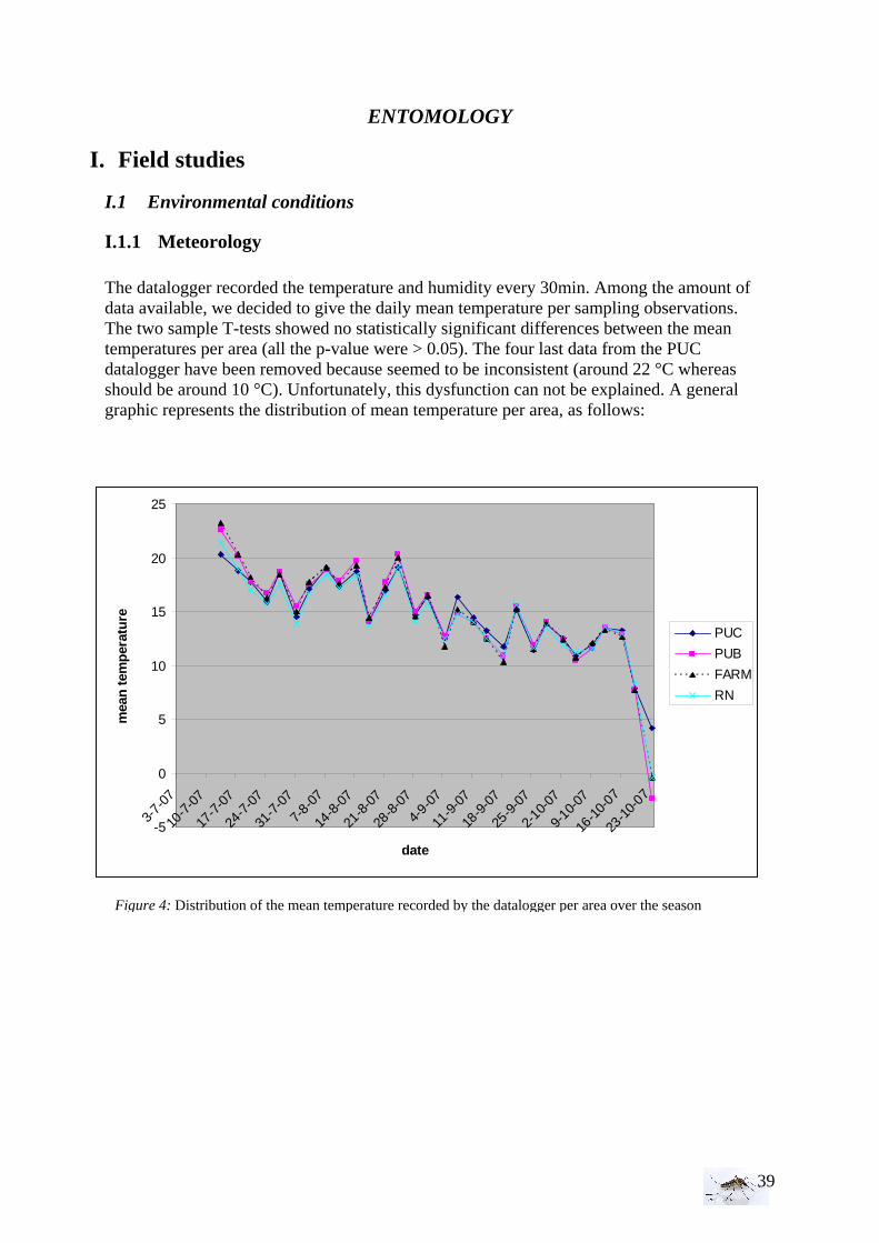
39

ENTOMOLOGY

I. Field studies

I.1 Environmental conditions

I.1.1 Meteorology The datalogger recorded the temperature and humidity every 30min. Among the amount of data available, we decided to give the daily mean temperature per sampling observations. The two sample T-tests showed no statistically significant differences between the mean temperatures per area (all the p-value were > 0.05). The four last data from the PUC datalogger have been removed because seemed to be inconsistent (around 22 °C whereas should be around 10 °C). Unfortunately, this dysfunction can not be explained. A general graphic represents the distribution of mean temperature per area, as follows:

Figure 4: Distribution of the mean temperature recorded by the datalogger per area over the season

-5

0

5

10

15

20

25

3-7-0

7

10-7

-07

17-7

-07

24-7

-07

31-7

-07

7-8-0

7

14-8

-07

21-8

-07

28-8

-07

4-9-0

7

11-9

-07

18-9

-07

25-9

-07

2-10-

07

9-10-

07

16-1

0-07

23-1

0-07

date

mea

n te

mpe

ratu

re

PUC

PUB

FARM

RN

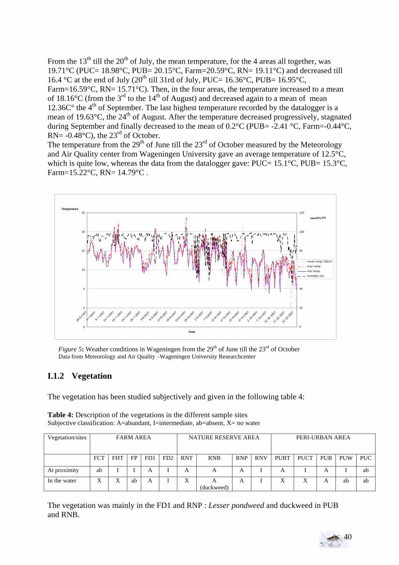
40

From the 13th till the 20th of July, the mean temperature, for the 4 areas all together, was 19.71°C (PUC= 18.98°C, PUB= 20.15°C, Farm=20.59°C, RN= 19.11°C) and decreased till 16.4 °C at the end of July (20th till 31rd of July, PUC= 16.36°C, PUB= 16.95°C, Farm=16.59°C, RN= 15.71°C). Then, in the four areas, the temperature increased to a mean of 18.16°C (from the 3rd to the 14th of August) and decreased again to a mean of mean 12.36C° the 4th of September. The last highest temperature recorded by the datalogger is a mean of 19.63°C, the 24th of August. After the temperature decreased progressively, stagnated during September and finally decreased to the mean of 0.2°C (PUB= -2.41 °C, Farm=-0.44°C, RN= -0.48°C), the 23rd of October. The temperature from the 29th of June till the 23rd of October measured by the Meteorology and Air Quality center from Wageningen University gave an average temperature of 12.5°C, which is quite low, whereas the data from the datalogger gave: PUC= 15.1°C, PUB= 15.3°C, Farm=15.22°C, RN= 14.79°C .

I.1.2 Vegetation The vegetation has been studied subjectively and given in the following table 4: Table 4: Description of the vegetations in the different sample sites Subjective classification: A=abundant, I=intermediate, ab=absent, X= no water Vegetation/sites FARM AREA NATURE RESERVE AREA PERI-URBAN AREA

FCT FHT FP FD1 FD2 RNT RNB RNP RNV PUBT PUCT PUB PUW PUC

At proximity ab I I A I A A A I A I A I ab

In the water X X ab A I X A (duckweed)

A I X X A ab ab

The vegetation was mainly in the FD1 and RNP : Lesser pondweed and duckweed in PUB and RNB.

Figure 5: Weather conditions in Wageningen from the 29th of June till the 23rd of October Data from Meteorology and Air Quality –Wageningen University Researchcenter

-5

0

5

10

15

20

25

29-6

-200

7

4-7-2

007

9-7-

2007

14-7

-200

7

19-7

-200

7

24-7

-200

7

29-7

-200

7

3-8-

2007

8-8-

2007

13-8

-200

7

18-8-

2007

23-8

-200

7

28-8

-200

7

2-9-

2007

7-9-2

007

12-9-

2007

17-9

-200

7

22-9

-200

7

27-9

-200

7

2-10

-200

7

7-10

-200

7

12-10

-200

7

17-1

0-20

07

22-1

0-20

07

Date

Temperature

0

20

40

60

80

100

120

Humidity (%)

mean temp 150cm

max temp

min temp

humidity (%)

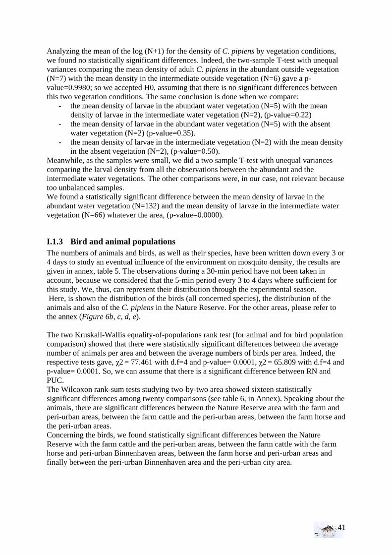
41

Analyzing the mean of the log (N+1) for the density of C. pipiens by vegetation conditions, we found no statistically significant differences. Indeed, the two-sample T-test with unequal variances comparing the mean density of adult C. pipiens in the abundant outside vegetation (N=7) with the mean density in the intermediate outside vegetation (N=6) gave a p-value=0.9980; so we accepted H0, assuming that there is no significant differences between this two vegetation conditions. The same conclusion is done when we compare:

- the mean density of larvae in the abundant water vegetation (N=5) with the mean density of larvae in the intermediate water vegetation (N=2), (p-value=0.22)

- the mean density of larvae in the abundant water vegetation (N=5) with the absent water vegetation (N=2) (p-value=0.35).

- the mean density of larvae in the intermediate vegetation (N=2) with the mean density in the absent vegetation (N=2), (p-value=0.50).

Meanwhile, as the samples were small, we did a two sample T-test with unequal variances comparing the larval density from all the observations between the abundant and the intermediate water vegetations. The other comparisons were, in our case, not relevant because too unbalanced samples. We found a statistically significant difference between the mean density of larvae in the abundant water vegetation (N=132) and the mean density of larvae in the intermediate water vegetation (N=66) whatever the area, (p-value=0.0000).

I.1.3 Bird and animal populations The numbers of animals and birds, as well as their species, have been written down every 3 or 4 days to study an eventual influence of the environment on mosquito density, the results are given in annex, table 5. The observations during a 30-min period have not been taken in account, because we considered that the 5-min period every 3 to 4 days where sufficient for this study. We, thus, can represent their distribution through the experimental season. Here, is shown the distribution of the birds (all concerned species), the distribution of the animals and also of the C. pipiens in the Nature Reserve. For the other areas, please refer to the annex (Figure 6b, c, d, e). The two Kruskall-Wallis equality-of-populations rank test (for animal and for bird population comparison) showed that there were statistically significant differences between the average number of animals per area and between the average numbers of birds per area. Indeed, the respective tests gave, χ2 = 77.461 with d.f=4 and p-value= 0.0001, χ2 = 65.809 with d.f=4 and p-value= 0.0001. So, we can assume that there is a significant difference between RN and PUC. The Wilcoxon rank-sum tests studying two-by-two area showed sixteen statistically significant differences among twenty comparisons (see table 6, in Annex). Speaking about the animals, there are significant differences between the Nature Reserve area with the farm and peri-urban areas, between the farm cattle and the peri-urban areas, between the farm horse and the peri-urban areas. Concerning the birds, we found statistically significant differences between the Nature Reserve with the farm cattle and the peri-urban areas, between the farm cattle with the farm horse and peri-urban Binnenhaven areas, between the farm horse and peri-urban areas and finally between the peri-urban Binnenhaven area and the peri-urban city area.

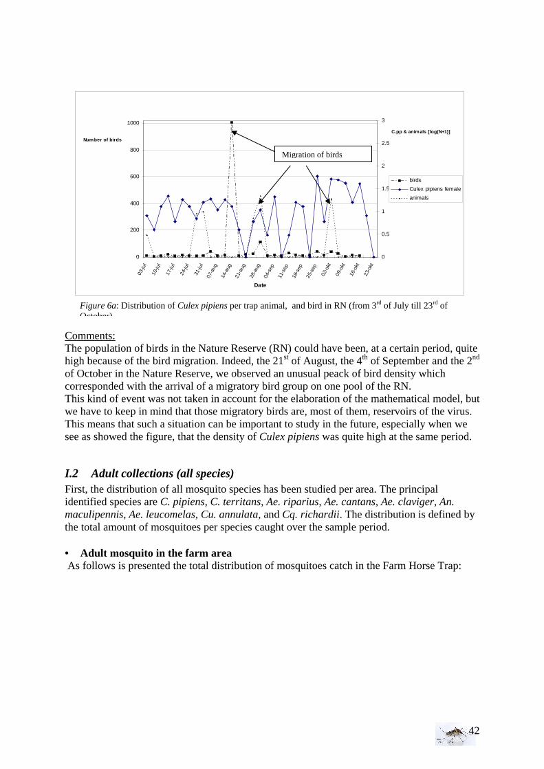
42

Comments: The population of birds in the Nature Reserve (RN) could have been, at a certain period, quite high because of the bird migration. Indeed, the 21st of August, the 4th of September and the 2nd of October in the Nature Reserve, we observed an unusual peack of bird density which corresponded with the arrival of a migratory bird group on one pool of the RN. This kind of event was not taken in account for the elaboration of the mathematical model, but we have to keep in mind that those migratory birds are, most of them, reservoirs of the virus. This means that such a situation can be important to study in the future, especially when we see as showed the figure, that the density of Culex pipiens was quite high at the same period.

I.2 Adult collections (all species) First, the distribution of all mosquito species has been studied per area. The principal identified species are C. pipiens, C. territans, Ae. riparius, Ae. cantans, Ae. claviger, An. maculipennis, Ae. leucomelas, Cu. annulata, and Cq. richardii. The distribution is defined by the total amount of mosquitoes per species caught over the sample period. • Adult mosquito in the farm area As follows is presented the total distribution of mosquitoes catch in the Farm Horse Trap:

0

200

400

600

800

1000

03-ju

l

10-ju

l

17-ju

l

24-ju

l

31-ju

l07

-aug

14-a

ug

21-a

ug

28-a

ug

04-s

ep

11-s

ep

18-s

ep

25-s

ep

02-o

kt

09-o

kt

16-o

kt

23-o

kt

Date

Number of birds

0

0.5

1

1.5

2

2.5

3

C.pp & animals [log(N+1)]

birds

Culex pipiens female

animals

Figure 6a: Distribution of Culex pipiens per trap animal, and bird in RN (from 3rd of July till 23rd of October)

Migration of birds

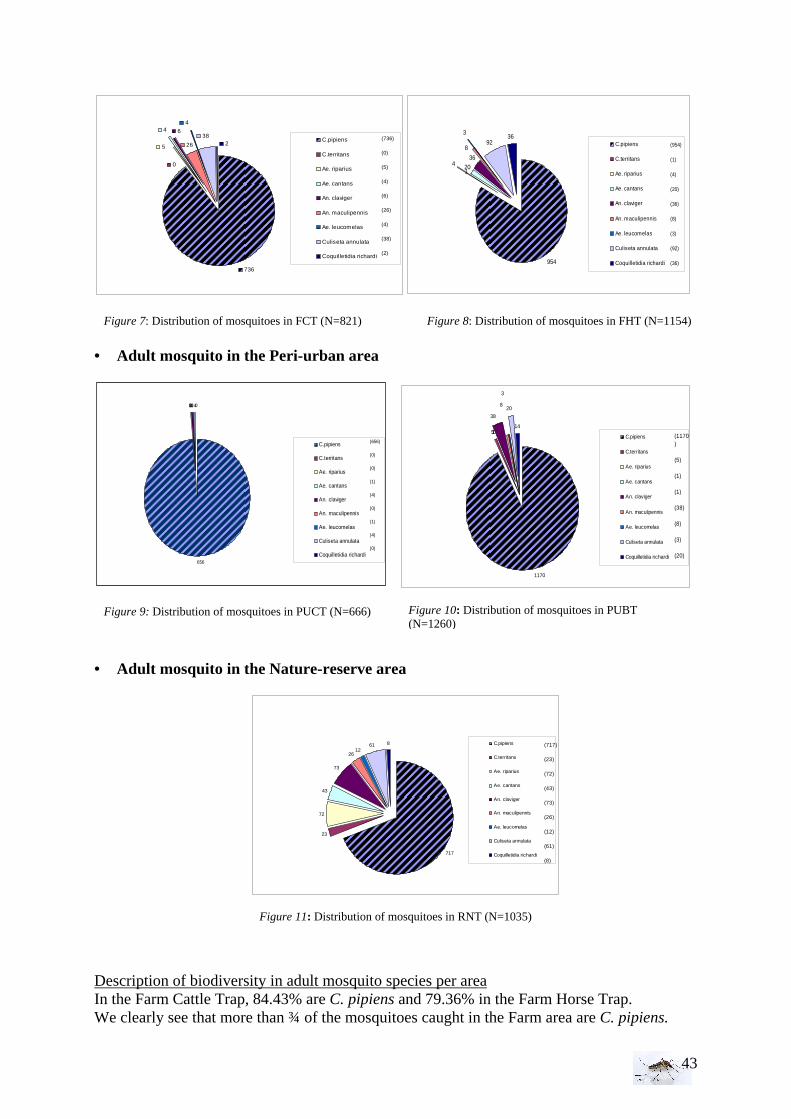
43

• Adult mosquito in the Peri-urban area

• Adult mosquito in the Nature-reserve area Description of biodiversity in adult mosquito species per area In the Farm Cattle Trap, 84.43% are C. pipiens and 79.36% in the Farm Horse Trap. We clearly see that more than ¾ of the mosquitoes caught in the Farm area are C. pipiens.

Figure 7: Distribution of mosquitoes in FCT (N=821)

238

4

26

64

5

0

736

C.pipiens

C.territans

Ae. riparius

Ae. cantans

An. claviger

An. maculipennis

Ae. leucomelas

Culiseta annulata

Coquilletidia richardi

(736)

(0)

(5)

(4)

(6)

(26)

(4)

(38)

(2)

3692

3

8

36

2041

954

C.pipiens

C.territans

Ae. riparius

Ae. cantans

An. claviger

An. maculipennis

Ae. leucomelas

Culiseta annulata


(954)

(1)

(4)

(20)

(36)

(8)

(3)

(92)

(36)

Figure 8: Distribution of mosquitoes in FHT (N=1154)

Figure 10: Distribution of mosquitoes in PUBT (N=1260)

Figure 9: Distribution of mosquitoes in PUCT (N=666)

1170

511

38

8

3

20

14

C.pipiens

C.territans

Ae. riparius

Ae. cantans

An. claviger

An. maculipennis

Ae. leucomelas

Culiseta annulata


(1170)

(5)

(1)

(1)

(38)

(8)

(3)

(20)656

00140140

C.pipiens

C.territans

Ae. riparius

Ae. cantans

An. claviger

An. maculipennis

Ae. leucomelas

Culiseta annulata


(656)

(0)

(0)

(1)

(4)

(0)

(1)

(4)

(0)

Figure 11: Distribution of mosquitoes in RNT (N=1035)

717

23

72

43

73

2612

61 8 C.pipiens

C.territans

Ae. riparius

Ae. cantans

An. claviger

An. maculipennis

Ae. leucomelas

Culiseta annulata


(717)

(23)

(72)

(43)

(73)

(26)

(12)

(61)

(8)

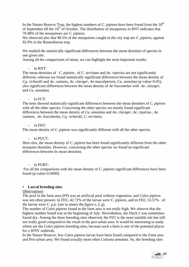
44

In the Nature Reserve Trap, the highest numbers of C. pipiens have been found from the 18th of September till the 16th of October. The distribution of mosquitoes in RNT indicates that 70.48% of the mosquitoes are C. pipiens. We observed also that 98.5% of the mosquitoes caught in the city trap are C. pipiens, against 92.9% in the Binnenhaven trap. We studied the statistically significant differences between the mean densities of species in one given site. Among all the comparisons of mean, we can highlight the most important results:

- in RNT: The mean densities of C. pipiens , of C. territans and Ae. riparius are not significantly different, whereas we found statistically significant differences between the mean density of Cq. richardii and Ae. cantans, Ae. claviger, An maculipennis, Cu. annulata (p-value<0.05), also significant differences between the mean density of Ae leucomelas with Ae. claviger, and Cu. annulata.

- in FCT: The tests showed statistically significant differences between the mean densities of C. pipiens with all the other species. Concerning the other species we mostly found significant differences between the mean density of Cu. annulata and An. claviger, Ae. riparius., Ae. cantans, Ae. leucomelas, Cq. richardii, C. territans.

- in FHT: The mean density of C. pipiens was significantly different with all the other species.

- in PUCT: Here also, the mean density of C. pipiens has been found significantly different from the other mosquito densities. However, concerning the other species we found no significant differences between its mean densities.

- in PUBT: For all the comparisons with the mean density of C. pipiens significant differences have been found (p-value=0.0000). • Larval breeding sites Observations: The pool in the farm area (FP) was an artificial pool without vegetation, and Culex pipiens was not often present. In FD1, 42.72% of the larvae were C. pipiens, and in FD2, 53.57% of the larvae were C. p.p. (see in annex the figure e, f, g). The number of Culex pipiens found in the farm area is not really high. We observe that the highest number found was at the beginning of July. Nevertheless, the Ditch 2 was sometimes found dry. Among the three breeding sites observed, the FD1 is the most suitable site but still not really good compared to the result in the peri-urban area. It would be interesting to study where are the Culex pipiens breeding sites, because such a farm is one of the potential places for a WNV outbreak. In the Nature Reserve, few Culex pipiens larvae have been found compared to the Farm area and Peri-urban area. We found actually more often Culiseta annulata. So, the breeding sites

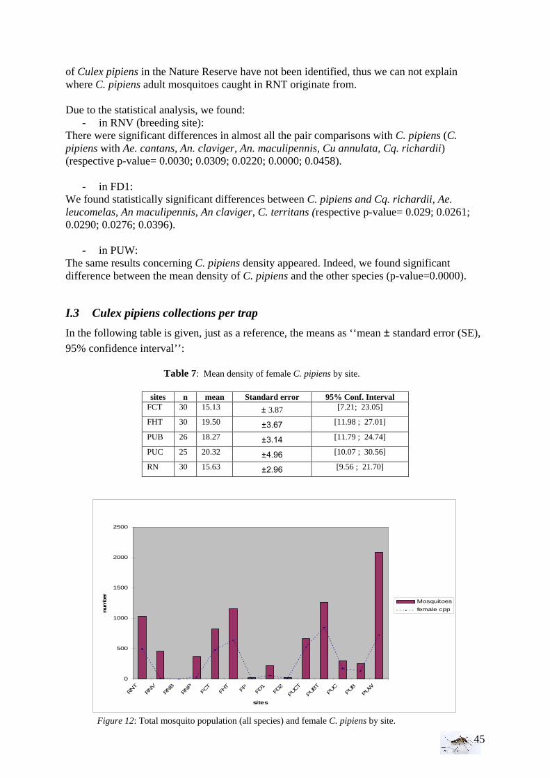
45

of Culex pipiens in the Nature Reserve have not been identified, thus we can not explain where C. pipiens adult mosquitoes caught in RNT originate from. Due to the statistical analysis, we found:

- in RNV (breeding site): There were significant differences in almost all the pair comparisons with C. pipiens (C. pipiens with Ae. cantans, An. claviger, An. maculipennis, Cu annulata, Cq. richardii) (respective p-value= 0.0030; 0.0309; 0.0220; 0.0000; 0.0458).

- in FD1: We found statistically significant differences between C. pipiens and Cq. richardii, Ae. leucomelas, An maculipennis, An claviger, C. territans (respective p-value= 0.029; 0.0261; 0.0290; 0.0276; 0.0396).

- in PUW: The same results concerning C. pipiens density appeared. Indeed, we found significant difference between the mean density of C. pipiens and the other species (p-value=0.0000).

I.3 Culex pipiens collections per trap

In the following table is given, just as a reference, the means as ‘‘mean ± standard error (SE), 95% confidence interval’’:

Table 7: Mean density of female C. pipiens by site.

sites n mean Standard error 95% Conf. Interval FCT 30 15.13 ± 3.87 [7.21; 23.05]

FHT 30 19.50 ±3.67 [11.98 ; 27.01]

PUB 26 18.27 ±3.14 [11.79 ; 24.74]

PUC 25 20.32 ±4.96 [10.07 ; 30.56]

RN 30 15.63 ±2.96 [9.56 ; 21.70]

Figure 12: Total mosquito population (all species) and female C. pipiens by site.

0

500

1000

1500

2000

2500

RNT

RNV

RNB

RNP

FCT

FHT

FP FD1

FD2

PUCT

PUBT

PUC

PUB

PUW

sites

num

ber

Mosquitoes

female cpp

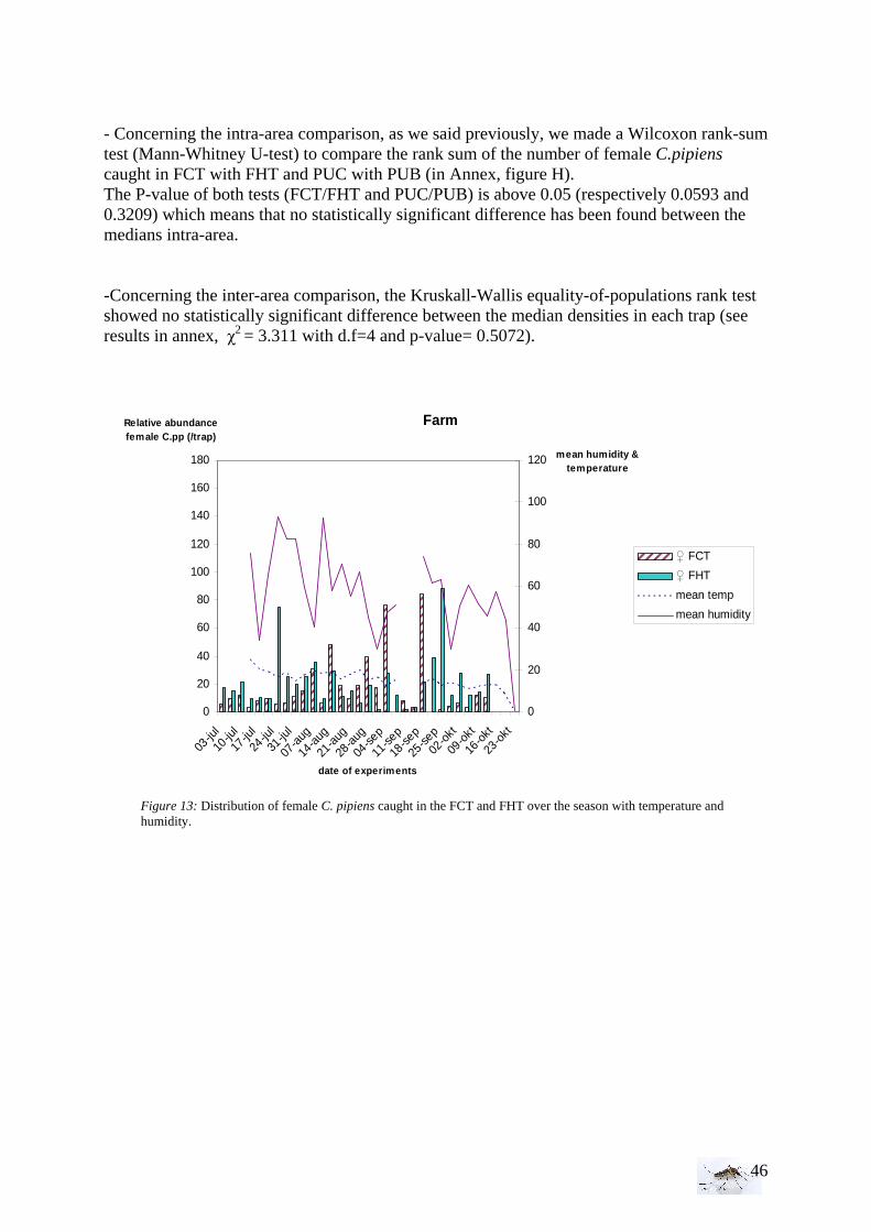
46

- Concerning the intra-area comparison, as we said previously, we made a Wilcoxon rank-sum test (Mann-Whitney U-test) to compare the rank sum of the number of female C.pipiens caught in FCT with FHT and PUC with PUB (in Annex, figure H). The P-value of both tests (FCT/FHT and PUC/PUB) is above 0.05 (respectively 0.0593 and 0.3209) which means that no statistically significant difference has been found between the medians intra-area. -Concerning the inter-area comparison, the Kruskall-Wallis equality-of-populations rank test showed no statistically significant difference between the median densities in each trap (see results in annex, χ2 = 3.311 with d.f=4 and p-value= 0.5072).

Farm

0

20

40

60

80

100

120

140

160

180

03-ju

l

10-ju

l

17-ju

l

24-ju

l

31-ju

l

07-a

ug

14-a

ug

21-a

ug

28-a

ug

04-se

p

11-se

p

18-se

p

25-se

p

02-o

kt

09-o

kt

16-o

kt

23-o

kt

date of experiments

Relative abundance female C.pp (/trap)

0

20

40

60

80

100

120 mean humidity & temperature

♀ FCT

♀ FHT

mean temp

mean humidity

Figure 13: Distribution of female C. pipiens caught in the FCT and FHT over the season with temperature and humidity.

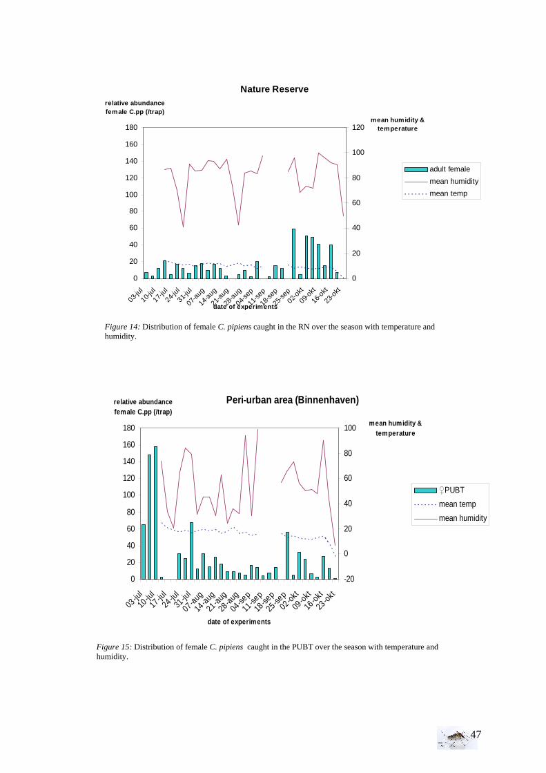
47

Nature Reserve

0

20

40

60

80

100

120

140

160

180

03-ju

l

10-ju

l

17-ju

l

24-ju

l

31-ju

l

07-a

ug

14-a

ug

21-a

ug

28-a

ug

04-s

ep

11-s

ep

18-s

ep

25-s

ep02

-okt

09-ok

t

16-o

kt

23-o

kt

date of experiments

relative abundance female C.pp (/trap)

0

20

40

60

80

100

120mean humidity &

temperature

adult female

mean humidity

mean temp

Figure 14: Distribution of female C. pipiens caught in the RN over the season with temperature and humidity.

Peri-urban area (Binnenhaven)

0

20

40

60

80

100

120

140

160

180

03-ju

l

10-ju

l

17-ju

l

24-ju

l

31-ju

l

07-au

g

14-au

g

21-au

g

28-au

g

04-se

p

11-se

p

18-se

p

25-se

p02

-okt

09-ok

t

16-ok

t

23-ok

t

date of experiments


-20

0

20

40

60

80

100mean humidity &

temperature

♀PUBT

mean temp

mean humidity

Figure 15: Distribution of female C. pipiens caught in the PUBT over the season with temperature and humidity.

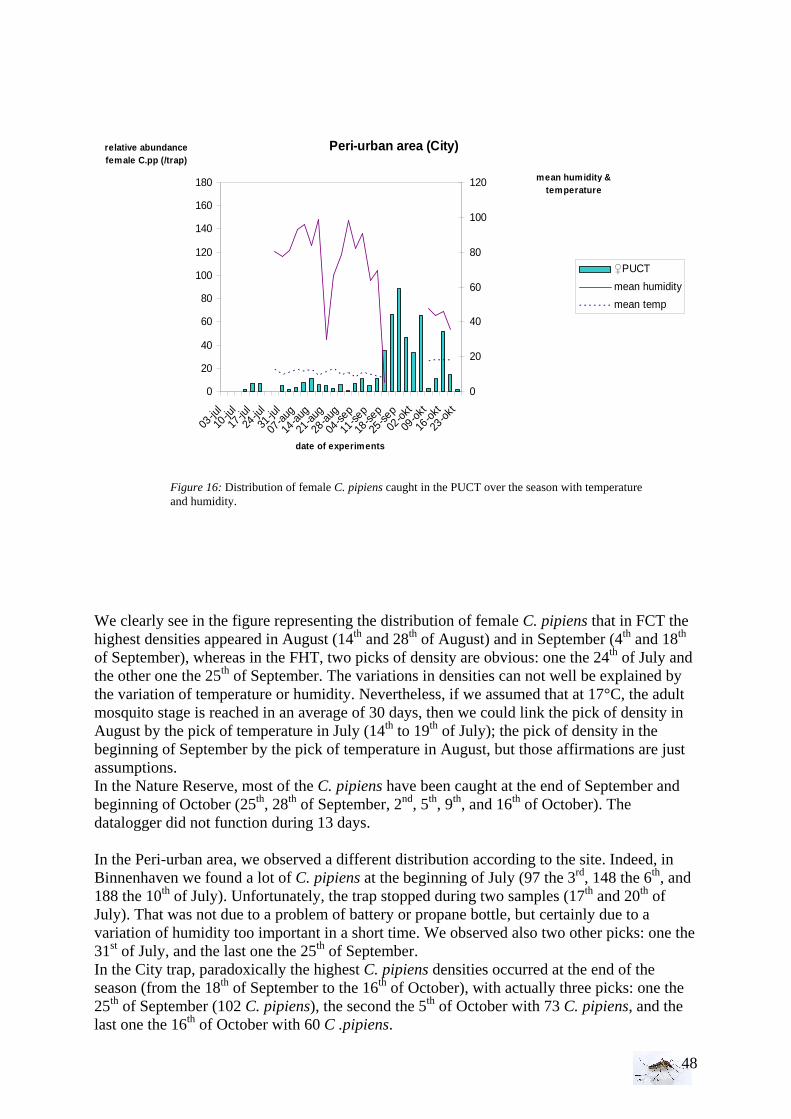
48

We clearly see in the figure representing the distribution of female C. pipiens that in FCT the highest densities appeared in August (14th and 28th of August) and in September (4th and 18th of September), whereas in the FHT, two picks of density are obvious: one the 24th of July and the other one the 25th of September. The variations in densities can not well be explained by the variation of temperature or humidity. Nevertheless, if we assumed that at 17°C, the adult mosquito stage is reached in an average of 30 days, then we could link the pick of density in August by the pick of temperature in July (14th to 19th of July); the pick of density in the beginning of September by the pick of temperature in August, but those affirmations are just assumptions. In the Nature Reserve, most of the C. pipiens have been caught at the end of September and beginning of October (25th, 28th of September, 2nd, 5th, 9th, and 16th of October). The datalogger did not function during 13 days. In the Peri-urban area, we observed a different distribution according to the site. Indeed, in Binnenhaven we found a lot of C. pipiens at the beginning of July (97 the 3rd, 148 the 6th, and 188 the 10th of July). Unfortunately, the trap stopped during two samples (17th and 20th of July). That was not due to a problem of battery or propane bottle, but certainly due to a variation of humidity too important in a short time. We observed also two other picks: one the 31st of July, and the last one the 25th of September. In the City trap, paradoxically the highest C. pipiens densities occurred at the end of the season (from the 18th of September to the 16th of October), with actually three picks: one the 25th of September (102 C. pipiens), the second the 5th of October with 73 C. pipiens, and the last one the 16th of October with 60 C .pipiens.

Peri-urban area (City)

0

20

40

60

80

100

120

140

160

180

03-ju

l

10-ju

l

17-ju

l

24-ju

l

31-ju

l

07-au

g

14-au

g

21-au

g

28-au

g

04-se

p

11-se

p

18-se

p

25-se

p

02-ok

t

09-ok

t

16-ok

t

23-ok

t

date of experiments


0

20

40

60

80

100

120 mean humidity & temperature

♀PUCT

mean humidity

mean temp

Figure 16: Distribution of female C. pipiens caught in the PUCT over the season with temperature and humidity.

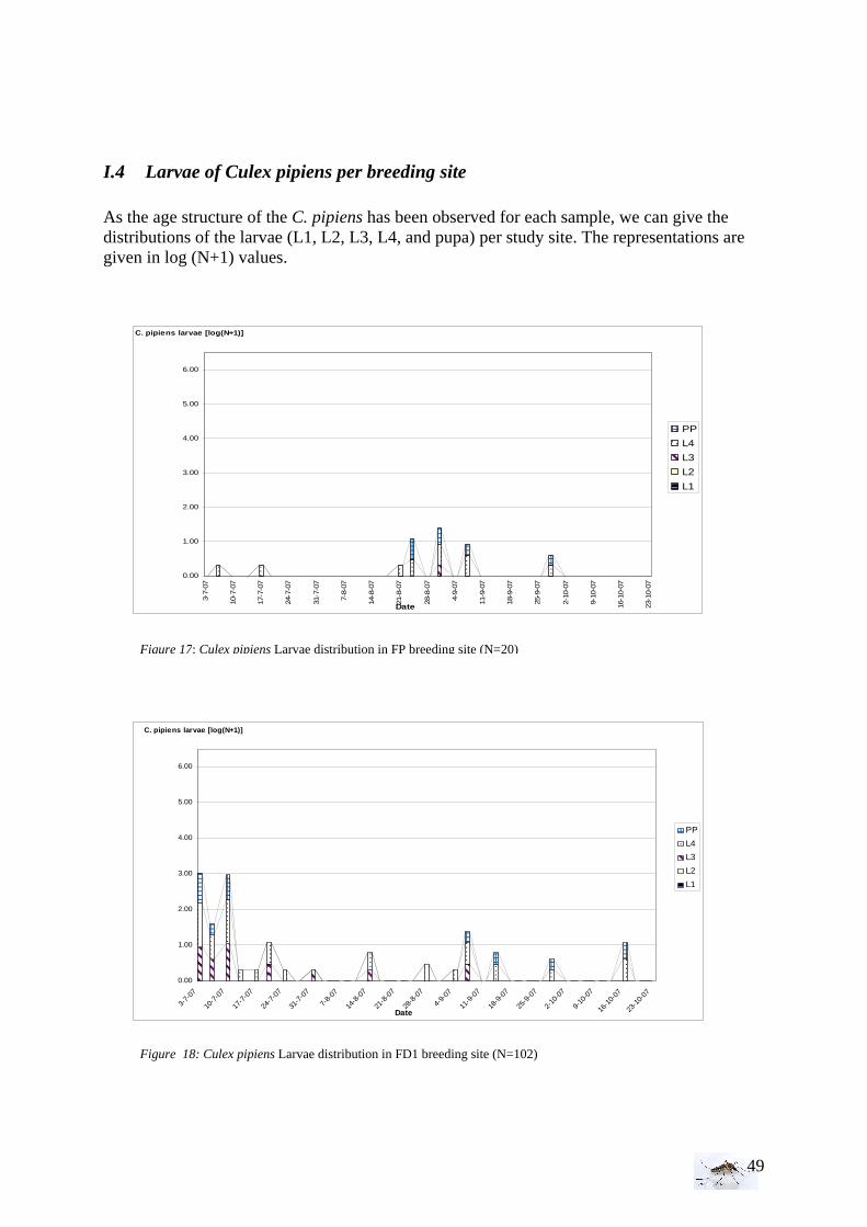
49

I.4 Larvae of Culex pipiens per breeding site As the age structure of the C. pipiens has been observed for each sample, we can give the distributions of the larvae (L1, L2, L3, L4, and pupa) per study site. The representations are given in log (N+1) values.

Figure 18: Culex pipiens Larvae distribution in FD1 breeding site (N=102)

0.00

1.00

2.00

3.00

4.00

5.00

6.00

3-7-

07

10-7

-07

17-7

-07

24-7

-07

31-7

-07

7-8-

07

14-8

-07

21-8

-07

28-8

-07

4-9-

07

11-9

-07

18-9

-07

25-9

-07

2-10

-07

9-10

-07

16-1

0-07

23-1

0-07

Date

C. pipiens larvae [log(N+1)]

PP

L4

L3

L2

L1

Figure 17: Culex pipiens Larvae distribution in FP breeding site (N=20)

0.00

1.00

2.00

3.00

4.00

5.00

6.00

3-7-

07

10-7

-07

17-7

-07

24-7

-07

31-7

-07

7-8-

07

14-8

-07

21-8

-07

28-8

-07

4-9-

07

11-9

-07

18-9

-07

25-9

-07

2-10

-07

9-10

-07

16-1

0-07

23-1

0-07

Date


PP

L4

L3

L2

L1

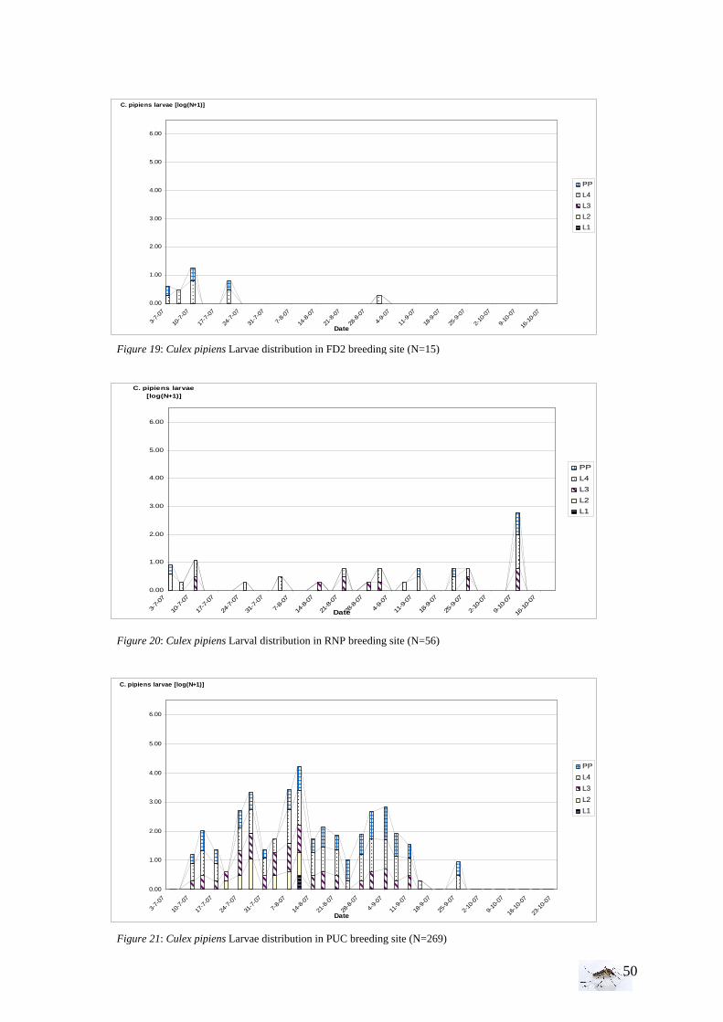
50

Figure 19: Culex pipiens Larvae distribution in FD2 breeding site (N=15)

0.00

1.00

2.00

3.00

4.00

5.00

6.00

3-7-

07

10-7

-07

17-7

-07

24-7

-07

31-7

-07

7-8-

07

14-8

-07

21-8

-07

28-8

-07

4-9-

07

11-9

-07

18-9

-07

25-9

-07

2-10

-07

9-10

-07

16-1

0-07

Date


PP

L4

L3

L2

L1

0.00

1.00

2.00

3.00

4.00

5.00

6.00

3-7-

07

10-7

-07

17-7

-07

24-7

-07

31-7

-07

7-8-

07

14-8

-07

21-8

-07

28-8

-07

4-9-

07

11-9

-07

18-9

-07

25-9

-07

2-10

-07

9-10

-07

16-1

0-07

23-1

0-07

Date


PP

L4

L3

L2

L1

Figure 21: Culex pipiens Larvae distribution in PUC breeding site (N=269)

Figure 20: Culex pipiens Larval distribution in RNP breeding site (N=56)

0.00

1.00

2.00

3.00

4.00

5.00

6.00

3-7-07

10-7-0

7

17-7-0

7

24-7-0

7

31-7

-07

7-8-

07

14-8

-07

21-8

-07

28-8

-07

4-9-

07

11-9

-07

18-9

-07

25-9

-07

2-10

-07

9-10

-07

16-1

0-07

Date


PP

L4

L3

L2

L1

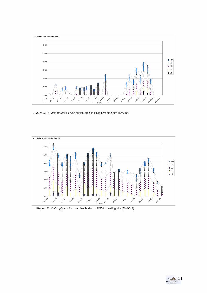
51

Figure 22 : Culex pipiens Larvae distribution in PUB breeding site (N=210)

0.00

1.00

2.00

3.00

4.00

5.00

6.00

3-7-

07

10-7

-07

17-7

-07

24-7

-07

31-7

-07

7-8-

07

14-8

-07

21-8

-07

28-8

-07

4-9-

07

11-9

-07

18-9

-07

25-9

-07

2-10

-07

9-10

-07

16-1

0-07

23-1

0-07

Date


PP

L4

L3

L2

L1

Figure 23: Culex pipiens Larvae distribution in PUW breeding site (N=2048)

0.00

1.00

2.00

3.00

4.00

5.00

6.00

3-7-

07

10-7

-07

17-7

-07

24-7

-07

31-7

-07

7-8-

07

14-8

-07

21-8

-07

28-8

-07

4-9-

07

11-9

-07

18-9

-07

25-9

-07

2-10

-07

Date


PP

L4

L3

L2

L1

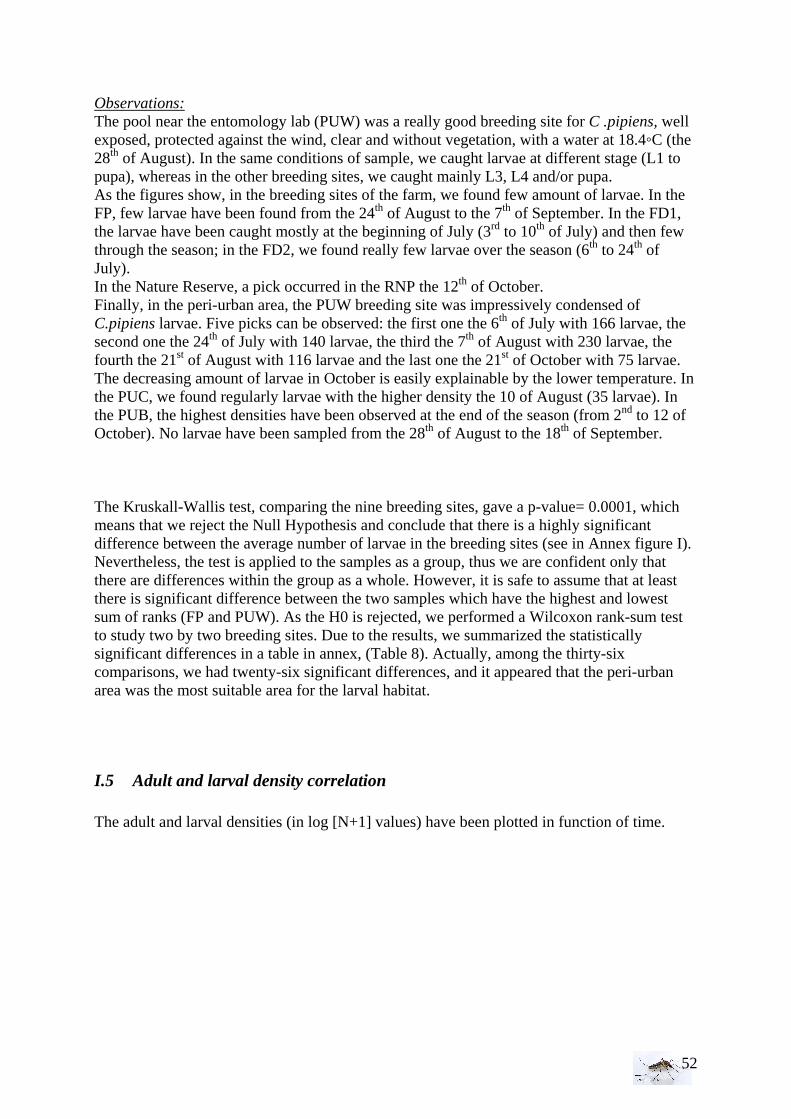
52

Observations: The pool near the entomology lab (PUW) was a really good breeding site for C .pipiens, well exposed, protected against the wind, clear and without vegetation, with a water at 18.4◦C (the 28th of August). In the same conditions of sample, we caught larvae at different stage (L1 to pupa), whereas in the other breeding sites, we caught mainly L3, L4 and/or pupa. As the figures show, in the breeding sites of the farm, we found few amount of larvae. In the FP, few larvae have been found from the 24th of August to the 7th of September. In the FD1, the larvae have been caught mostly at the beginning of July (3rd to 10th of July) and then few through the season; in the FD2, we found really few larvae over the season (6th to 24th of July). In the Nature Reserve, a pick occurred in the RNP the 12th of October. Finally, in the peri-urban area, the PUW breeding site was impressively condensed of C.pipiens larvae. Five picks can be observed: the first one the 6th of July with 166 larvae, the second one the 24th of July with 140 larvae, the third the 7th of August with 230 larvae, the fourth the 21st of August with 116 larvae and the last one the 21st of October with 75 larvae. The decreasing amount of larvae in October is easily explainable by the lower temperature. In the PUC, we found regularly larvae with the higher density the 10 of August (35 larvae). In the PUB, the highest densities have been observed at the end of the season (from 2nd to 12 of October). No larvae have been sampled from the 28th of August to the 18th of September. The Kruskall-Wallis test, comparing the nine breeding sites, gave a p-value= 0.0001, which means that we reject the Null Hypothesis and conclude that there is a highly significant difference between the average number of larvae in the breeding sites (see in Annex figure I). Nevertheless, the test is applied to the samples as a group, thus we are confident only that there are differences within the group as a whole. However, it is safe to assume that at least there is significant difference between the two samples which have the highest and lowest sum of ranks (FP and PUW). As the H0 is rejected, we performed a Wilcoxon rank-sum test to study two by two breeding sites. Due to the results, we summarized the statistically significant differences in a table in annex, (Table 8). Actually, among the thirty-six comparisons, we had twenty-six significant differences, and it appeared that the peri-urban area was the most suitable area for the larval habitat.

I.5 Adult and larval density correlation The adult and larval densities (in log [N+1] values) have been plotted in function of time.

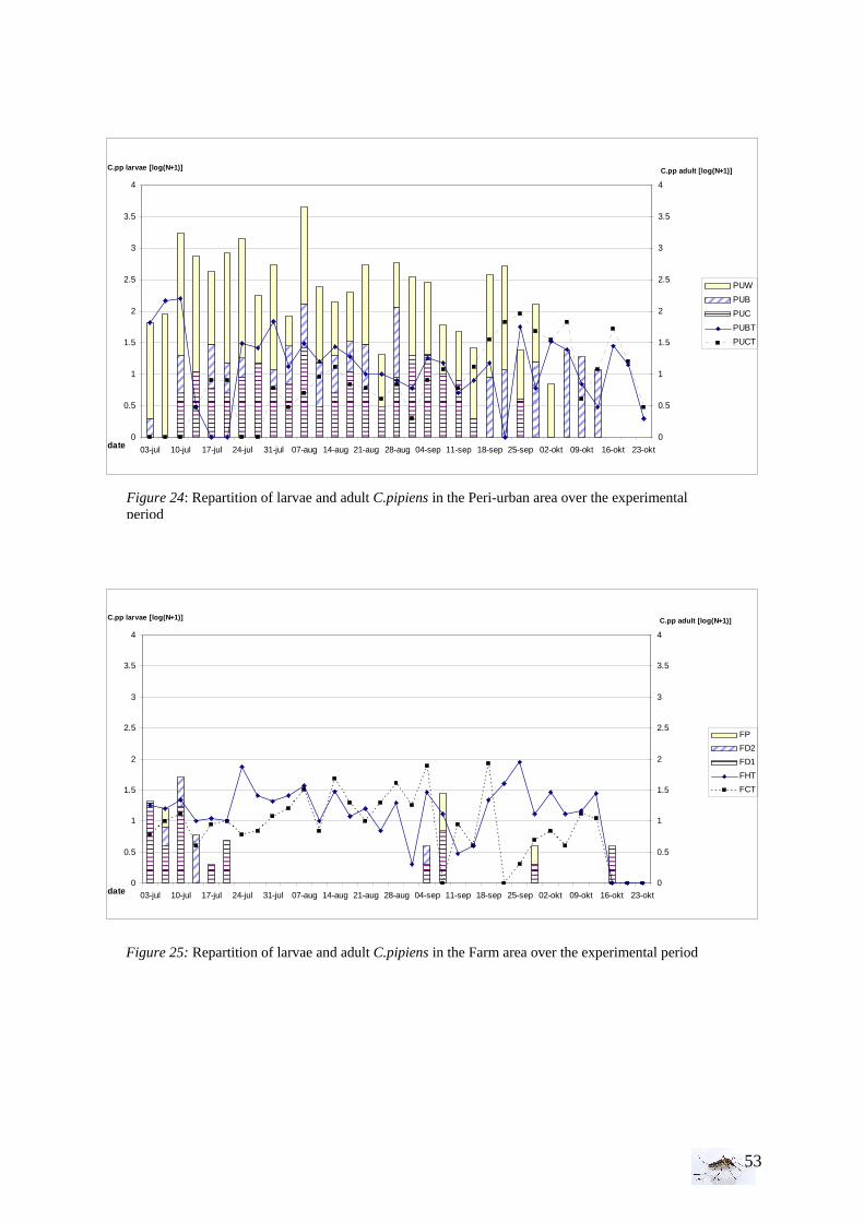
53

0

0.5

1

1.5

2

2.5

3

3.5

4

03-jul 10-jul 17-jul 24-jul 31-jul 07-aug 14-aug 21-aug 28-aug 04-sep 11-sep 18-sep 25-sep 02-okt 09-okt 16-okt 23-oktdate

C.pp larvae [log(N+1)]

0

0.5

1

1.5

2

2.5

3

3.5

4

C.pp adult [log(N+1)]

FP

FD2

FD1

FHT

FCT

Figure 25: Repartition of larvae and adult C.pipiens in the Farm area over the experimental period

0

0.5

1

1.5

2

2.5

3

3.5

4



0

0.5

1

1.5

2

2.5

3

3.5

4

C.pp adult [log(N+1)]

PUW

PUB

PUC

PUBT

PUCT

Figure 24: Repartition of larvae and adult C.pipiens in the Peri-urban area over the experimental period

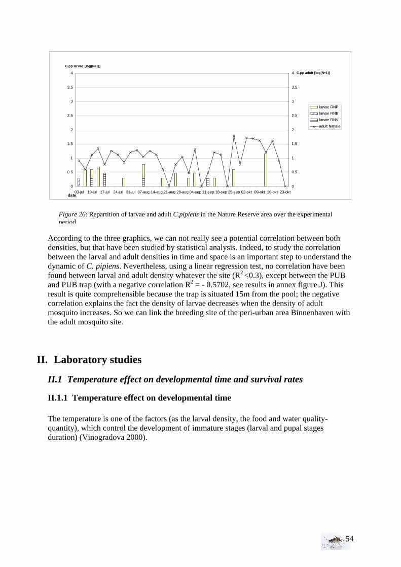
54

According to the three graphics, we can not really see a potential correlation between both densities, but that have been studied by statistical analysis. Indeed, to study the correlation between the larval and adult densities in time and space is an important step to understand the dynamic of C. pipiens. Nevertheless, using a linear regression test, no correlation have been found between larval and adult density whatever the site (R2 <0.3), except between the PUB and PUB trap (with a negative correlation R2 = - 0.5702, see results in annex figure J). This result is quite comprehensible because the trap is situated 15m from the pool; the negative correlation explains the fact the density of larvae decreases when the density of adult mosquito increases. So we can link the breeding site of the peri-urban area Binnenhaven with the adult mosquito site.

II. Laboratory studies

II.1 Temperature effect on developmental time and survival rates

II.1.1 Temperature effect on developmental time The temperature is one of the factors (as the larval density, the food and water quality-quantity), which control the development of immature stages (larval and pupal stages duration) (Vinogradova 2000).

0

0.5

1

1.5

2

2.5

3

3.5

4



0

0.5

1

1.5

2

2.5

3

3.5

4 C.pp adult [log(N+1)]

larvae RNP

larvae RNB

larvae RNV

adult female

Figure 26: Repartition of larvae and adult C.pipiens in the Nature Reserve area over the experimental period

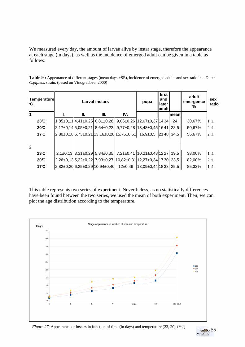
55

We measured every day, the amount of larvae alive by instar stage, therefore the appearance at each stage (in days), as well as the incidence of emerged adult can be given in a table as follows: Table 9 : Appearance of different stages (mean days ±SE), incidence of emerged adults and sex ratio in a Dutch C.pipiens strain. (based on Vinogradova, 2000)

Temperature °C

Larval instars pupa

first and later adult

adult

emergence %

sex ratio

1 I. II. III. IV. mean

23°C 1,85±0,11 4,41±0,25 6,81±0,28 9,06±0,26 12,67±0,37 14 34 24 30,67% 1 :1

20°C 2,17±0,14 5,05±0,21 8,64±0,22 9,77±0,28 13,48±0,45 16 41 28,5 50,67% 2 :1

17°C 2,80±0,18 6,73±0,21 13,16±0,28 15,76±0,51 16,9±0,5 21 48 34,5 56,67% 2 :1

2

23°C 2,1±0,13 3,31±0,29 5,84±0,35 7,21±0,41 10,21±0,48 12 27 19,5 38,00% 1 :1

20°C 2,26±0,13 5,22±0,22 7,93±0,27 10,82±0,31 12,27±0,34 17 30 23,5 82,00% 2 :1

17°C 2,82±0,20 6,25±0,29 10,94±0,40 12±0,46 13,09±0,44 18 33 25,5 85,33% 1 :1

This table represents two series of experiment. Nevertheless, as no statistically differences have been found between the two series, we used the mean of both experiment. Then, we can plot the age distribution according to the temperature.

II.1.2 Temperature effect on survival rates

II.1.3 Wings length/temperature correlation

I. II. III. IV. pupa first later adult

0

5

10

15

20

25

30

35

40

45

Stage appearance in function of time and temperature

23°C

20°C

17°C

Days

Figure 27: Appearance of instars in function of time (in days) and temperature (23, 20, 17°C)

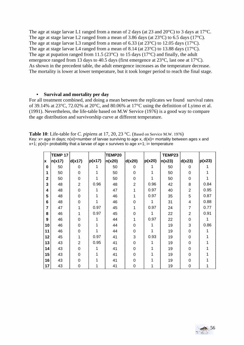
56

The age at stage larvae L1 ranged from a mean of 2 days (at 23 and 20°C) to 3 days at 17°C. The age at stage larvae L2 ranged from a mean of 3.86 days (at 23°C) to 6.5 days (17°C). The age at stage larvae L3 ranged from a mean of 6.33 (at 23°C) to 12.05 days (17°C). The age at stage larvae L4 ranged from a mean of 8.14 (at 23°C) to 13.88 days (17°C). The age at pupation ranged from 11.5 (23°C) to 15 days (17°C) and finally, the adult emergence ranged from 13 days to 40.5 days (first emergence at 23°C, last one at 17°C). As shown in the precedent table, the adult emergence increases as the temperature decrease. The mortality is lower at lower temperature, but it took longer period to reach the final stage.

• Survival and mortality per day For all treatment combined, and doing a mean between the replicates we found survival rates of 39.14% at 23°C, 72.02% at 20°C, and 80.06% at 17°C using the definition of Lyimo et al. (1991). Nevertheless, the life-table based on M.W Service (1976) is a good way to compare the age distribution and survivorship curve at different temperature. Table 10: Life-table for C. pipiens at 17, 20, 23 °C. (Based on Service M.W. 1976) Key: x= age in days; n(xi)=number of larvae surviving to age x, d(xi)= mortality between ages x and x+1; p(xi)= probability that a larvae of age x survives to age x+1; i= temperature

TEMP 17 TEMP20 TEMP23

x n(x17) d(x17) p(x17) n(x20) d(x20) p(x20) n(x23) d(x23) p(x23) 0 50 0 1 50 0 1 50 0 1

1 50 0 1 50 0 1 50 0 1

2 50 0 1 50 0 1 50 0 1

3 48 2 0.96 48 2 0.96 42 8 0.84

4 48 0 1 47 1 0.97 40 2 0.95

5 48 0 1 46 1 0.97 35 5 0.87

6 48 0 1 46 0 1 31 4 0.88

7 47 1 0.97 45 1 0.97 24 7 0.77

8 46 1 0.97 45 0 1 22 2 0.91

9 46 0 1 44 1 0.97 22 0 1

10 46 0 1 44 0 1 19 3 0.86

11 46 0 1 44 0 1 19 0 1

12 45 1 0.97 41 3 0.93 19 0 1

13 43 2 0.95 41 0 1 19 0 1

14 43 0 1 41 0 1 19 0 1

15 43 0 1 41 0 1 19 0 1

16 43 0 1 41 0 1 19 0 1 17 43 0 1 41 0 1 19 0 1

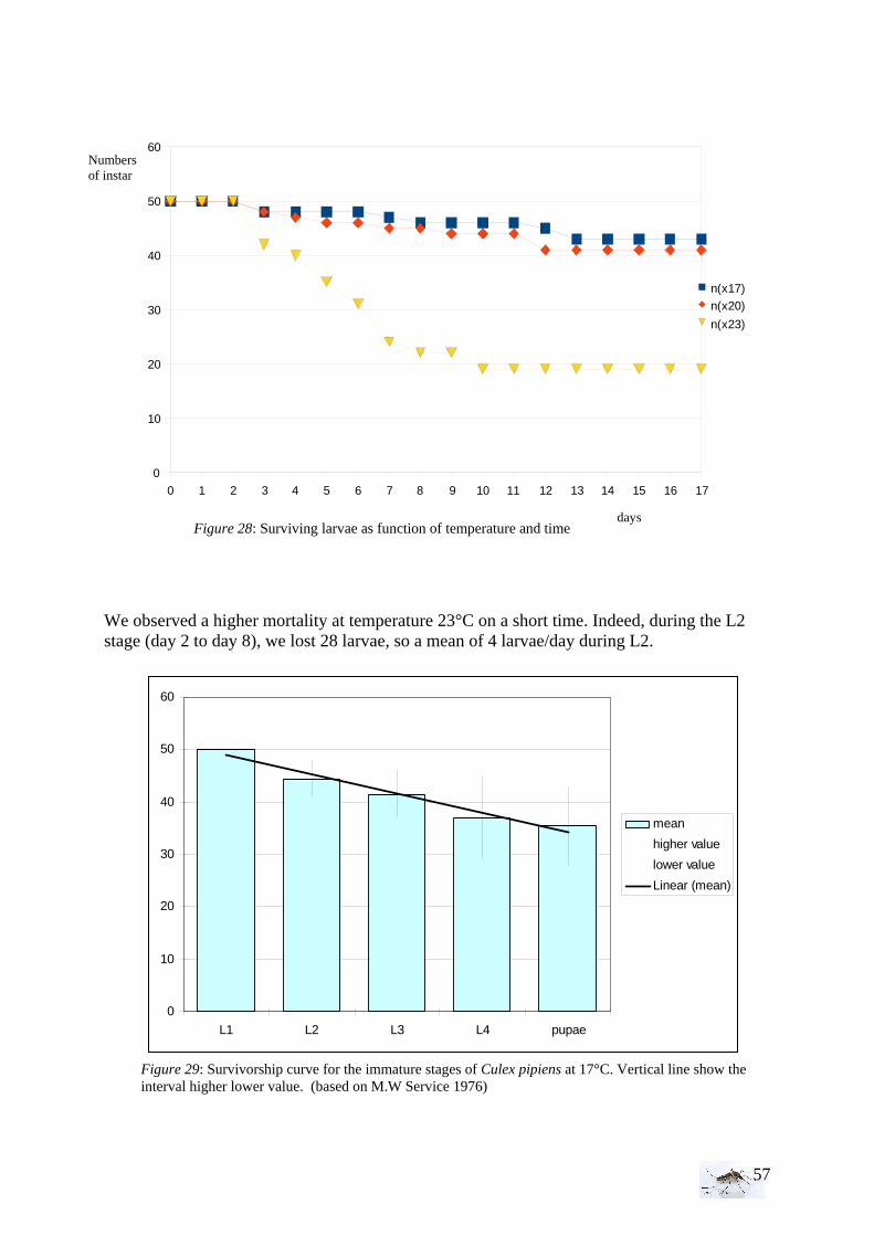
57

We observed a higher mortality at temperature 23°C on a short time. Indeed, during the L2 stage (day 2 to day 8), we lost 28 larvae, so a mean of 4 larvae/day during L2.

Figure 28: Surviving larvae as function of temperature and time

0 1 2 3 4 5 6 7 8 9 10 11 12 13 14 15 16 17

0

10

20

30

40

50

60

n(x17)

n(x20)

n(x23)

Numbers of instar

days

0

10

20

30

40

50

60

L1 L2 L3 L4 pupae

mean

higher value

lower value

Linear (mean)

Figure 29: Survivorship curve for the immature stages of Culex pipiens at 17°C. Vertical line show the interval higher lower value. (based on M.W Service 1976)

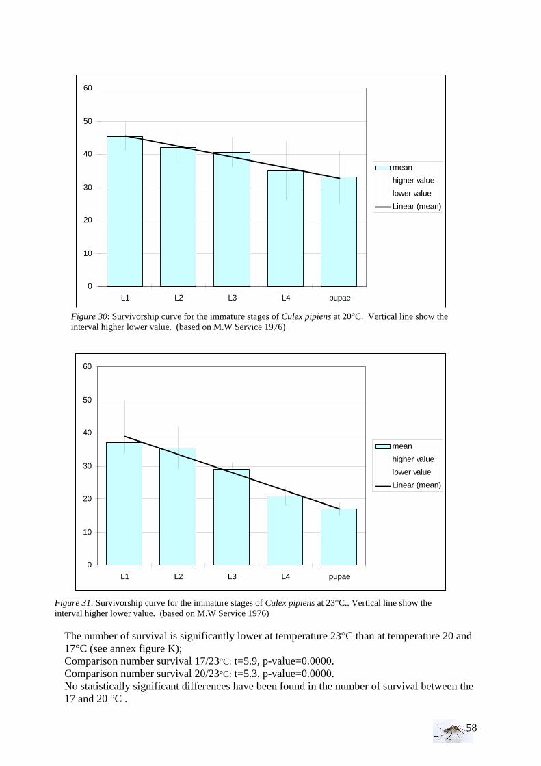
58

The number of survival is significantly lower at temperature 23°C than at temperature 20 and 17°C (see annex figure K); Comparison number survival 17/23°C: t=5.9, p-value=0.0000. Comparison number survival 20/23°C: t=5.3, p-value=0.0000. No statistically significant differences have been found in the number of survival between the 17 and 20 °C .

0

10

20

30

40

50

60

L1 L2 L3 L4 pupae

mean

higher value

lower value

Linear (mean)

Figure 30: Survivorship curve for the immature stages of Culex pipiens at 20°C. Vertical line show the interval higher lower value. (based on M.W Service 1976)

0

10

20

30

40

50

60

L1 L2 L3 L4 pupae

mean

higher value

lower value

Linear (mean)

Figure 31: Survivorship curve for the immature stages of Culex pipiens at 23°C.. Vertical line show the interval higher lower value. (based on M.W Service 1976)

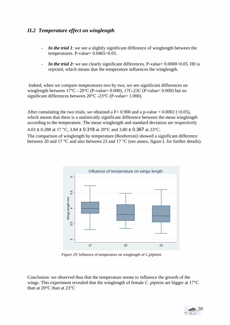
59

II.2 Temperature effect on winglength

- In the trial 1: we see a slightly significant difference of winglength between the temperatures. P-value= 0.0465<0.05.

- In the trial 2: we see clearly significant differences. P-value= 0.0000<0.05. H0 is

rejected, which means that the temperature influences the winglength. Indeed, when we compare temperatures two by two, we see significant differences on winglength between 17°C - 20°C (P-value= 0.000), 17C-23C (P-value= 0.000) but no significant differences between 20°C -23°C (P-value= 1.000). After cumulating the two trials, we obtained a F= 0.900 and a p-value = 0.0002 (<0.05), which means that there is a statistically significant difference between the mean winglength according to the temperature. The mean winglength and standard deviation are respectively

4.03 ± 0.288 at 17 °C, 3.84 ± 0.318 at 20°C and 3.80 ± 0.367 at 23°C. The comparison of winglength by temperature (Bonferroni) showed a significant difference between 20 and 17 °C and also between 23 and 17 °C (see annex, figure L for further details). Conclusion: we observed thus that the temperature seems to influence the growth of the wings. This experiment revealed that the winglength of female C .pipiens are bigger at 17°C than at 20°C than at 23°C

33.

54

4.5

5W

ings

leng

th m

m

17 20 23

Influence of temperature on wings length

Figure 29: Influence of temperature on winglength of C.pipiens

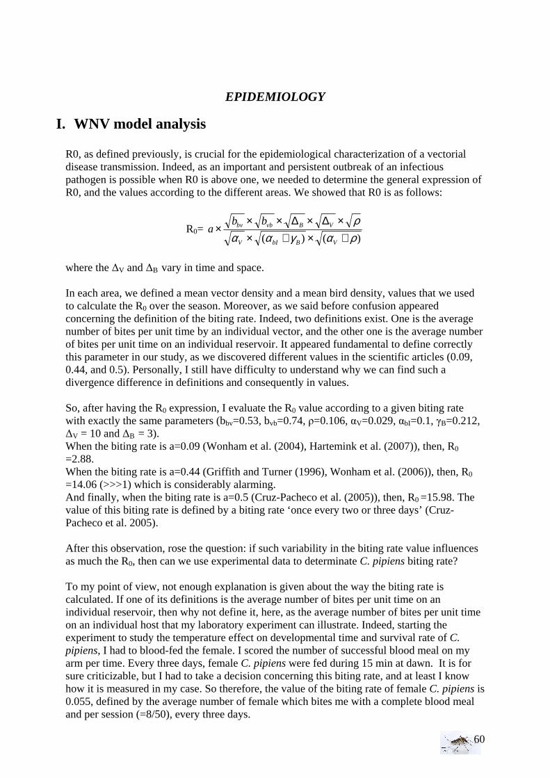
60

EPIDEMIOLOGY

I. WNV model analysis R0, as defined previously, is crucial for the epidemiological characterization of a vectorial disease transmission. Indeed, as an important and persistent outbreak of an infectious pathogen is possible when R0 is above one, we needed to determine the general expression of R0, and the values according to the different areas. We showed that R0 is as follows:

R0= )()( ραγαα

ρ+×+×

×∆×∆×××

VBbIV

VBvbbv bba

where the ∆V and ∆B vary in time and space. In each area, we defined a mean vector density and a mean bird density, values that we used to calculate the R0 over the season. Moreover, as we said before confusion appeared concerning the definition of the biting rate. Indeed, two definitions exist. One is the average number of bites per unit time by an individual vector, and the other one is the average number of bites per unit time on an individual reservoir. It appeared fundamental to define correctly this parameter in our study, as we discovered different values in the scientific articles (0.09, 0.44, and 0.5). Personally, I still have difficulty to understand why we can find such a divergence difference in definitions and consequently in values. So, after having the R0 expression, I evaluate the R0 value according to a given biting rate with exactly the same parameters (bbv=0.53, bvb=0.74, ρ=0.106, αV=0.029, αbI=0.1, γB=0.212, ∆V = 10 and ∆B = 3). When the biting rate is a=0.09 (Wonham et al. (2004), Hartemink et al. (2007)), then, R0

=2.88. When the biting rate is a=0.44 (Griffith and Turner (1996), Wonham et al. (2006)), then, R0

=14.06 (>>>1) which is considerably alarming. And finally, when the biting rate is a=0.5 (Cruz-Pacheco et al. (2005)), then, R0 =15.98. The value of this biting rate is defined by a biting rate ‘once every two or three days’ (Cruz-Pacheco et al. 2005). After this observation, rose the question: if such variability in the biting rate value influences as much the R0, then can we use experimental data to determinate C. pipiens biting rate? To my point of view, not enough explanation is given about the way the biting rate is calculated. If one of its definitions is the average number of bites per unit time on an individual reservoir, then why not define it, here, as the average number of bites per unit time on an individual host that my laboratory experiment can illustrate. Indeed, starting the experiment to study the temperature effect on developmental time and survival rate of C. pipiens, I had to blood-fed the female. I scored the number of successful blood meal on my arm per time. Every three days, female C. pipiens were fed during 15 min at dawn. It is for sure criticizable, but I had to take a decision concerning this biting rate, and at least I know how it is measured in my case. So therefore, the value of the biting rate of female C. pipiens is 0.055, defined by the average number of female which bites me with a complete blood meal and per session (=8/50), every three days.

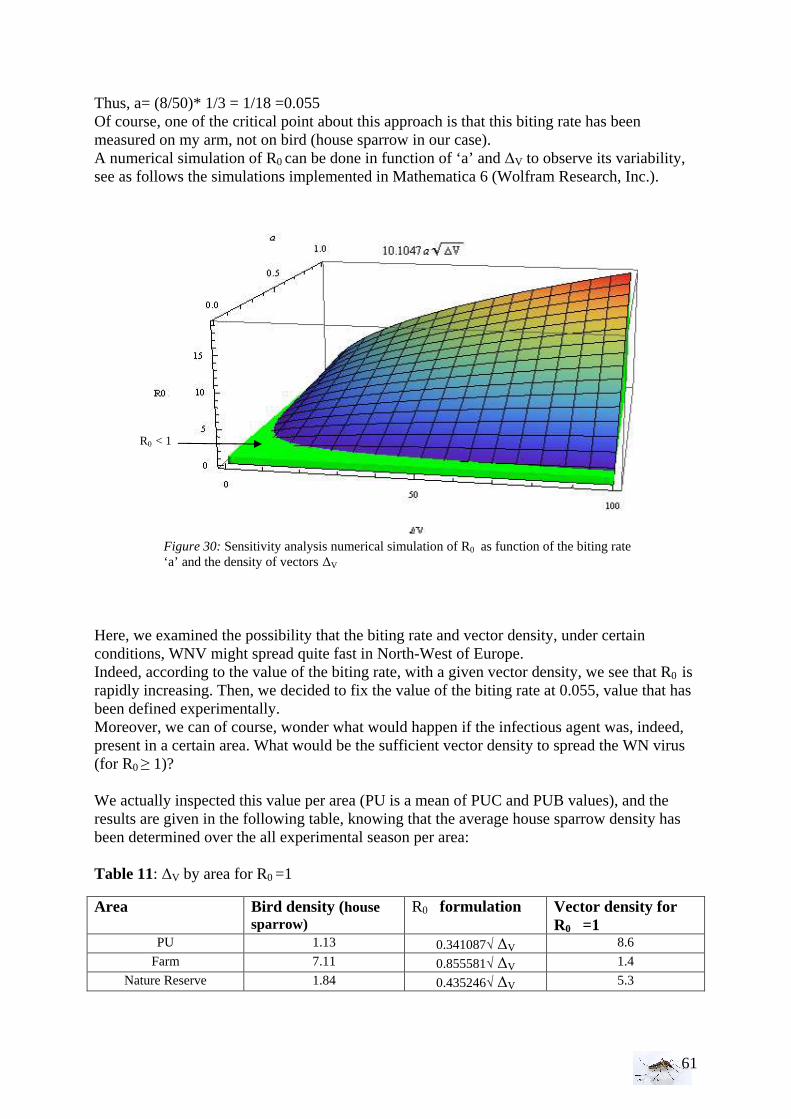
61

Thus, a= (8/50)* 1/3 = 1/18 =0.055 Of course, one of the critical point about this approach is that this biting rate has been measured on my arm, not on bird (house sparrow in our case). A numerical simulation of R0 can be done in function of ‘a’ and ∆V to observe its variability, see as follows the simulations implemented in Mathematica 6 (Wolfram Research, Inc.). Here, we examined the possibility that the biting rate and vector density, under certain conditions, WNV might spread quite fast in North-West of Europe. Indeed, according to the value of the biting rate, with a given vector density, we see that R0 is rapidly increasing. Then, we decided to fix the value of the biting rate at 0.055, value that has been defined experimentally. Moreover, we can of course, wonder what would happen if the infectious agent was, indeed, present in a certain area. What would be the sufficient vector density to spread the WN virus (for R0 ≥ 1)? We actually inspected this value per area (PU is a mean of PUC and PUB values), and the results are given in the following table, knowing that the average house sparrow density has been determined over the all experimental season per area: Table 11: ∆V by area for R0 =1

Area Bird density (house sparrow)

R0 formulation Vector density for R0 =1

PU 1.13 0.341087√ ∆V 8.6

Farm 7.11 0.855581√ ∆V 1.4

Nature Reserve 1.84 0.435246√ ∆V 5.3

Figure 30: Sensitivity analysis numerical simulation of R0 as function of the biting rate ‘a’ and the density of vectors ∆V

R0 < 1

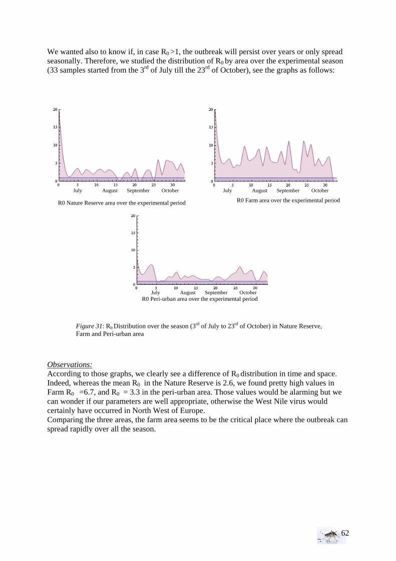
62

We wanted also to know if, in case R0 >1, the outbreak will persist over years or only spread seasonally. Therefore, we studied the distribution of R0 by area over the experimental season (33 samples started from the 3rd of July till the 23rd of October), see the graphs as follows: Observations: According to those graphs, we clearly see a difference of R0 distribution in time and space. Indeed, whereas the mean R0 in the Nature Reserve is 2.6, we found pretty high values in Farm R0 =6.7, and R0 = 3.3 in the peri-urban area. Those values would be alarming but we can wonder if our parameters are well appropriate, otherwise the West Nile virus would certainly have occurred in North West of Europe. Comparing the three areas, the farm area seems to be the critical place where the outbreak can spread rapidly over all the season.

R0 Nature Reserve area over the experimental period

R0 Peri-urban area over the experimental period

R0 Farm area over the experimental period

July August September October July August September October

July August September October

Figure 31: R0 Distribution over the season (3rd of July to 23rd of October) in Nature Reserve, Farm and Peri-urban area

63

II. WNV model predictions With the mathematical model, we can predict the R0 in time and space.

The critical stages appear to be quite spread during the season but mostly in the farm area. We observed, as seen previously, the difference of R0 distribution over space and time, and notice quite clearly the predisposition of the farm area to be an outbreak place. It is even more an important knowing that dead-end hosts as human and horses are present in this area. We can see that at the beginning and at the end of the season the R0 was quite close for all three areas (1< R0 <7), due to the fact that at this moment the vector density was higher in the Nature Reserve and Peri-urban area and lower in the farm than through all the season.

One of the essential issues of realizing a mathematical model is to predict when and where the potential outbreak can occur. Thus, on the same map (Figure 33), are represented the different class of R0 over the season. If an infected bird occurred in the Farm, for example, at the beginning of July, we see that the reproduction number is already quite high and then, can predict an endemic situation. We can also expect a propagation if we consider that birds and vectors can fly from area to area (till 3.5km for C. pipiens). Thus, if the pathogen agent appears in the farm area, it could spread via the trajectory of birds or vectors to the city and to the Nature Reserve areas. In the peri-urban area (suburban area), during 13 weeks in the season, there is a lower probability that the outbreak can occur, but one time more, everything depends on plenty of parameters. Let’s take the week 10: if infected vectors or bird fly to the city area, the probability of outbreak is lower than if it flew to the Nature reserve this same week. In contrary, during

R0[t] per area

0.00

1.00

2.00

3.00

4.00

5.00

6.00

7.00

8.00

9.00

10.00

11.00

12.00

1 2 3 4 5 6 7 8 9 10 11 12 13 14 15 16 17 18 19 20 21 22 23 24 25 26 27 28 29 30 31 32 33

sample time

R0

RN

F

PU

Figure 32: R0 distribution in time and space over the season

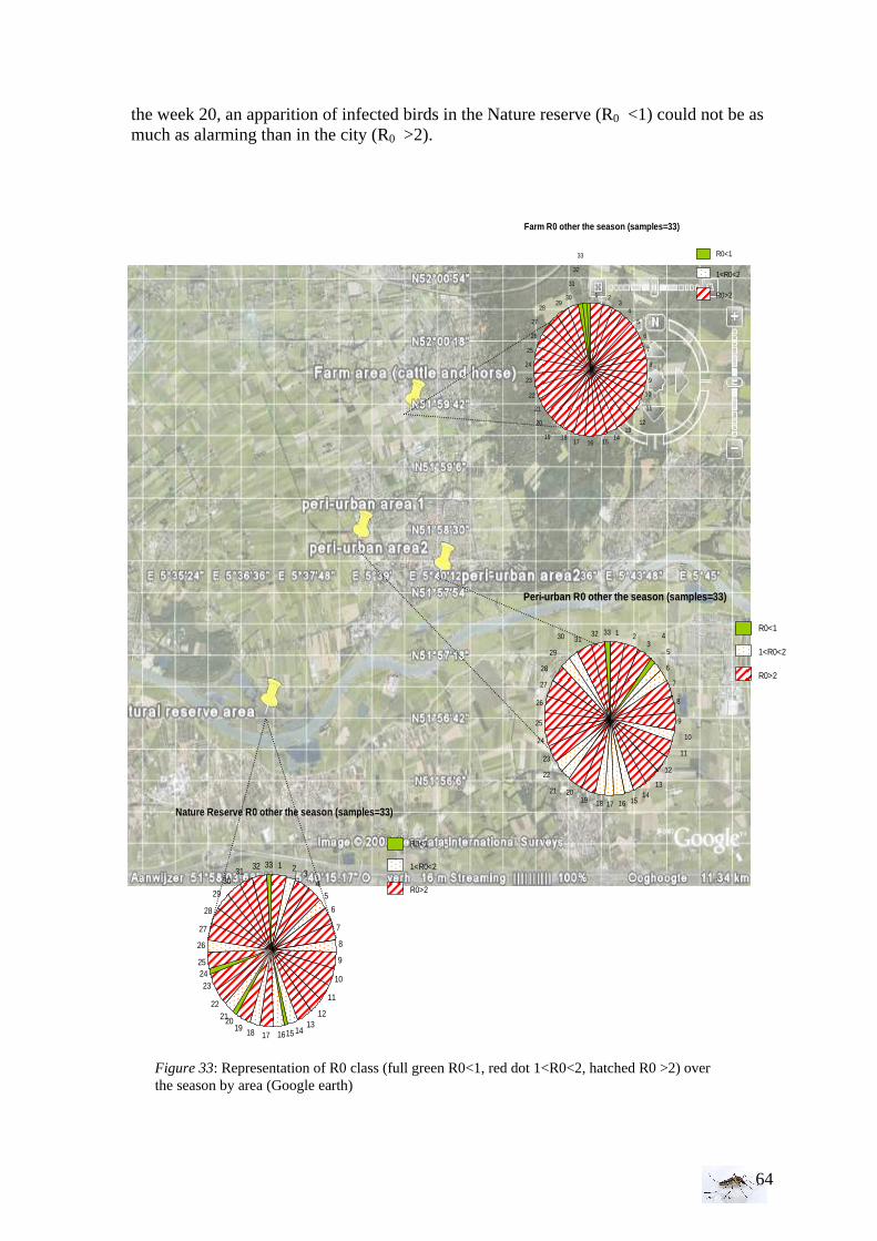
64

the week 20, an apparition of infected birds in the Nature reserve (R0 <1) could not be as much as alarming than in the city (R0 >2).

Nature Reserve R0 other the season (samples=33)

1 23

45

6

7

8

9

10

11

1213

1415161718192021

22

232425

26

27

28

29

3031

32 33

R0<1

1<R0<2

R0>2

Farm R0 other the season (samples=33)

1 23

4

5

6

7

8

9

10

11

1213

14151617

1819

20

21

22

23

24

25

26

27

2829

30

31

32

33 R0<1

1<R0<2

R0>2

Peri-urban R0 other the season (samples=33)

1 23

4

5

6

7

8

9

10

11

12

1314

15161718192021

22

23

24

25

26

27

28

29

30 3132 33 R0<1

1<R0<2

R0>2

Figure 33: Representation of R0 class (full green R0<1, red dot 1<R0<2, hatched R0 >2) over the season by area (Google earth)

65

FOURTH PART:

DISCUSSION AND CONCLUSIONS

66

I. Discussions

EPIDEMIOLOGY The factors which can lead to a fast and persistent spread of WNV through Africa, Eurasia, North America are still not well understood even if incredible progress have been made. Undoubtedly, the vector density, bird and vector competence as well as the virus replication in birds, are known as prerequisites for the transmission and persistence of WNV (Foppa et al. 2007). Unfortunately, the vector density is not defined in the same way by all the authors. That made the model comparison even more complex. We choose to define the vector and bird density as the number of individual by a given area and during a certain time, whereas some authors define it just as a number. But we know that a flight range of a bird is not comparable to a flight range of a mosquito, the conditions of observation are also different. Here, we predicted, given certain parameters, the WNV risks in North West Europe. We had to determine several parameters, as the vector density, the bird density (house sparrow) by area, as well as the C. pipiens maturation rate and find the best and appropriate biting rate. We assumed that C. pipiens bite and blood feed at a constant rate, but we know that avian defensive behavior has an impact on the blood-feeding success of C. pipiens (Darbro et al. 2007) and this will make that the biting rate per mosquito at high densities of the mosquitoes will be lower. Concerning the biting rate, we had a difficulty to define this parameter and by doing a sensitivity analysis, we realized its importance. Of course the way it has been estimated in our study can highly be criticize but at least, it is based on real (experimental) data. The space parameter (area) has been included in the model, in the way that the vector and bird densities were not the same between areas. This parameter is really important in a model and we would expect, with more time, to predict the WNV spread from area to area. The different areas (habitats) were quite represented in this study, even if the city zone was not so easy to study (breeding site dry sooner than the other sites). Indeed, I had to face the problem of dry breeding sites, and when it occurred at the end of the study, it is even more problematic because you can not change to another site. At the beginning of the model building process, I choose to include all bird species, but it appeared to be too complicated when I had to select a value for the bird mortality rate or for the transmission probability of WNV from bird to vector for all the different bird species. Then, as the house sparrow is a common bird in North West of Europe and a competent reservoir of WNV, I decided to reduce the bird species to Passer domesticus. Darbro et al (2007) showed that even intra-bird species, significant differences have been

found concerning the mosquito blood-feeding success (estimate= 0.0167 ± 0.00902, Z= 1.85, p=0.0319). The defensive behavior of a bird would be also an interesting parameter to take in account but for that we would have need much more time to consider it in the model. This parameter may increase the frequency of host contact (Foppa et al. 2007). Darbro et al. (2007) found differences in success of C. pipiens pipiens between bird species. Indeed, feeding success of C. pipiens pipiens on house sparrows was measured to be 82%, this is higher than the feeding success of other mosquito species. Variations in biting rate, in biting resistance on birds, in

67

mosquito density, in tolerance threshold in different populations of birds may influence the blood-feeding success (Darbro et al. 2007).

A big bird can, in one way, be suspected to be more resistant to the virus than a little bird , with a thicker skin making the blood feeding success low, and in the other hand if the bird has a larger body surface then it offers more opportunities to the vector to bite resulting in a higher infectious. This assumption has to be verified but it would also be interesting to create a model for a certain category of bird. The WNV competence index has been studied for eight species of birds by Cruz-Pacheco et al. (2005). This study showed that a Blue jay is more competent for the WNV than, respectively, an American crow, a house sparrow or a fish crow. We can also question about the WNV mortality, are the bigger birds more resistant? How is the transmission? The before mentioned study also has given the WNV mortality (day-

1) and the transmission probability. The highest transmission probability is 0.68 for the Blue jay with a WNV mortality (0.15 day-1), whereas the transmission probability is 0.26 for the Fish crow with a WNV mortality of 0.06 day-1. So we can wonder what would have been the prediction with another common bird as crow, for example. Ladeau et al. (2007) showed the mortality is likely to facilitate WNV amplification. The infectiousness of hosts (magnitude of viraemia and length of viral shedding) is lower in individuals that survive relative to those that die, and hosts that die from infections are not present as immune or dead-end hosts. The vector to host ratio is also increased by mortality, which increases the reproductive ratio of the pathogen, R0. Moreover, a diminution in host abundance can influence WNV transmission. For example, if house sparrow population decreases, it could implicate higher incidences of mosquitoes feeding on humans and intensified human WNV epidemics.

We did not speak about the variation of the WNV virulence in our study but we know that the strain of WNV varies in virulence. Indeed, the one circulating in Africa and Eurasia can be less virulent than the one introduced into North America.

• Public Health implications If the virus can persist in the reservoir and vector populations, it is a worst case for the dead-end hosts. The model we have presented predicts this for all areas for the average densities over the season and for most of the time during the season when we use the actual densities. However, we have not yet modeled how big the infected bird population would become within one season and what would happen between seasons. Moreover, we think that better estimates of (successful) biting rates are needed. We understand the importance of predicting a risk for public health and WNV has not caused, yet, epidemics in NW Europe but it seems that all the adequate conditions are present for such epidemics to occur.

• Future perspectives We estimated, by field and laboratory experiments, several parameters as the mosquito larval mortality rate, the vector and bird densities, the sex ratio and biting rate, but the model would have been even more precise if we would manage to estimate all the parameters. This temporal and spatial model could be improved by dynamic modelling including environmental aspects (as climate change, vegetations, and habitat). Environmental and ecological factors are indeed fundamental parameters. As we have shown that the possibilities for WNV to disseminate vary in time and place, it would be important to calculate how large epidemics could become after an introduction of WNV. Such model would need to account

68

for the total numbers that become infected (both of birds and vectors) and also their spatial pattern: how extensive is the area and thus are different habitats differently hit? Thus we understood, that a lot has still to be done to understand the occurrence of this virus, but several research program started already since 8 years and gives good perspectives.

ENTOMOLOGY

This study has shown that the Culex pipiens occured proportionally to the others species more in the Farm and Peri-urban area than in the Nature Reserve area. Larvae occurred more often in the PUW pool which was a breeding site without vegetation, clear water, and temperature quite warm compare to the other sites. As the conditions were not always perfect (dry pool0, we recommend to repeat this study with, perhaps, other pool or more on a longer period. The study of water conductivity, pH, and temperature has not been exploited to show differences among the breeding sites; two data sets are considered too small, but it is a good indication to take in account anyway, as we know already that temperature is a developmental time factor for larvae (Vinagradova 2000). We did not show a correlation between the density of larvae and the density of adult in the different areas, except in the Peri-urban area Binnenhaven which is quite comforting because the trap was situated close to the breeding site. It seems to be, indeed, hard to show on a short period where are the breeding sites of Culex pipiens, but it would be in the future an interesting perspective of study. The laboratory study enabled us to show that the temperature influences the developmental time of C .pipiens instar. We saw that it took more time for a larvae breed at 17°C to reach the adult stage than at 20 and 23°C; however more adults emerged at the lowest temperature. We can wonder why the lowest temperature is the best condition for a successful development. That result is even more important when we know that the average temperature in Wageningen in July till September is closer to 17°C than 20 °C (the average temperature during this experimental season was 12. 5°C). This study showed also that the number of survival per day is function of temperature. Actually at the highest temperature, the number of survival per day was lower. We can wonder if the larvae suffocate, if the water lost its quality. Finally, this study has shown that the temperature has an effect on the winglength of female C. pipiens, this result is in accord with the research of Vinogradova (2000). We, thus, can wonder what would be the fitness of the female C. pipiens in natural conditions; what would be the weight and the number of eggs per raft as function of temperature.

69

II. Conclusion The aim of this study was to develop and analyse a mathematical model to understand the dynamics of WNV disease and predict WNV risks associated with C. pipiens in North West of Europe. After the building of the model, an ecological study about the potential vector (C. pipiens) has been done enabling us to verify and improve our predictions. Preliminary results highlight the potential for transmission of the WNV outbreak over the season and we obtained conditions for the maintenance of the disease when the virus is introduced in certain locations: farm, sub-urban areas, nature reserve areas. We showed that the R0 increases with the C .pipiens density and with the biting rate. The main question would be why WNV has not occurred in North West of Europe as we calculated that all the necessary conditions for successful transmission are met (R0 >1). The control of WNV has become a priority in the South of France since 2001 and in the USA since 1999. Nevertheless, this control is still hard to achieve due to the large densities of susceptible vectors, of migratory birds and of other hosts. It is even more complex if we assume that vectors show vertical transmission and that direct bird to bird transmission occurs. The most likely scenario to maintain a disease free area would be to regularly check the absence of WNV virus, to regulate the vector density and improve the WNV model appropriate for climate and habitats changes.

70

REFERENCES

-Articles Anderson J.F., Andreadis T.G., Main A.J., Kline D.L. 2004. Prevalence of West Nile in tree canopy-inhabiting Culex pipiens and associated mosquitoes. Am.J.Trop.Med.Hyg. 71:112-119 Anderson J.F., Main A.J. 2006. Importance of vertical and horizontal transmission of West Nile virus by Culex pipiens in the Northeastern United States. Brief report in The Journal of Infectious Diseases. 194 : 1577-1579

Andreadis T.G., Anderson J.F., Vossbrinck C.R., Main A.J. 2004. Epidemiology of West Nile virus in Connecticut : a five-year analysis of mosquito data 1999-2003. Vector Borne Zoonotic Diseases. Winter; 4(4):360-378. Bakonyi T., Ivanics E., Erdélyi K., Ursu K., Ferenczi E., Weissenbock H., Nowotny N. 2006. Lineage 1 and 2 strains of Encephalitic West Nile Virus, Central Europe. Emerging Infectious Diseases. 12(4). Becker N,, Petríc D., Zgomba M., Boase C., Dahl C., Lane J., Kaiser A. 2003. Key to Female Mosquitoes. Extract from Mosquitoes and their control. Kluwer Academic Plenum Publishers, New York, 1rst Ed. Pp. xxi+498 Bernard K.A., Maffei J.G., Jones S.A., Kauffman E.B., Ebel D.G., Dupuis A.P., Ngo K.A., Nicholas D.C., Young D.M., Shi P-Y., Kulasekera V.L., Eidson M., White D.J., Stone W.B., NY State West Nile Virus Surveillance Team, Kramer L.D. 2001. West Nile virus infection in birds and mosquitoes, New York State, 2000. Emerging Infectious Diseases. 7(4). July-August Bowman C. 2005. A mathematical model for assessing control strategies against West Nile virus. Bull.Math.Biol . sept.; 67(5):1107-1133. Carrieri M., Bacchi M., Bellini R., Maini S. 2003. On the competition occurring between Aedes albopictus and Culex pipiens (Diptera: Culicidae) in Italy. Environmental Entomology. 32(6):1313-1321. Ceianu C.S., Ungureanu A., Nicolescu G., Cernescu C., Nitescu L., Tardei G., Petrescu A., Pitigoi D., Martin D., Ciulacu-Purcarea V., Vladimirescu A., Savage H.M. 2001. West Nile Virus surveillance in Romania : 1997-2000. Viral Immunol . 14(3):251-62. Cornel A.J., Jupp P.G., Blackburn N.K. 1993. Environmental temperature on the vector competence of Culex univittatus (Diptera: Culicidae) for West Nile virus. J.Med.Entomol. mar; 30(2):449-456 Cruz-Pacheco G., Esteva L., Montaňo-Hirose J.A., Vargas C. 2004. Modelling the dynamics of West Nile virus. Bulletin of Mathematical Biology. 67: 1157-1172.

71

Dauphin G., Zientara S., Zeller H., Murgue B. 2004. West Nile: Worldwide current situation in animals and humans. Comparative Immunology Microbiology and Infectious Diseases. 27(5):343-355. Darbro J.M., and Harrington L.C. 2007. Avian defensive behavior and blood-feeding success of the West Nile vector mosquito, Culex pipiens. Behavioral Ecology. 18:750-757. Dohm D.J., O’Guinn M.L., Turell M.J. 2002a. Effect of environmental temperature on the ability of Culex pipiens (Diptera:Culicidae) to transmit West Nile virus. J.Med.Entomol. Jan; 39(1):221-225 Dohm D.J., Sardelis M.R., Turell M.J. 2002. Experimental vertical transmission of West Nile virus by Culex pipiens (Diptera: Culicidae). Journal of Medical Entomology. 39(4) july:640-644 Ebel G.D., Carricaburu D., Young K.A. Kramer B & L.D. 2004. Genetic and phenotypic variation of West Nile virus in New York, 200-2003. American Journal of Tropical Medicine and Hygiene. 71: 493-500 Edman J.D., Webber L.A., Schmid A.A. 1974. Effect of host defenses on the feeding pattern of the Culex nigripalpus when offered a choice of blood sources. J.Parasitol. 60(5): 874-883 Emord D.E., Morris C.D. 1984. Epizootiology of eastern equine encephalomyelitis virus in upstate New York, USA, VI. Antibody prevalence in wild birds during an interepizootic period. J.Med.Entomol. 21:395-404 Foppa I.M., Spielman A. 2007. Does reservoir host mortality enhance transmission of West Nile virus? Theoretical Biology and Medical Modelling. 9 p Garrett-Jones C. 1964. The human blood index of Malaria vectors in relation to epidemiological assessment. Bull.World.Health Organ. 30:241-261 Gingrich J.B., Williams G.M. 2005. Host-feeding patterns of suspected West Nile virus mosquito vectors in Delaware, 2001-2002. Journal of the American Mosquito Control Association . 21(2): 194-200 Hethcote H.W. Wang W., and Li Y. 2005. Species coexistence and periodicity in host-host-pathogen models. J.Math.Biol. 51.:629-660. Hubalek Z., Halouzka J. 1999. West Nile Fever_ A re-emerging mosquito-borneviral disease in Europe [review]. Emerg.Infect.Dis.5:643-650. Hurlbut H.S. 1956. West Nile virus infection in arthropods. Am.J.Trop.Med.Hyg. 5(1):76-85 Jourdain E., Toussaint Y., Leblond A., Bicout D.J., Sabatier P., Gauthier-Clerc M. 2007. Bird species potentially involved in introduction, amplification and spread of West Nile virus in a Mediterranean wetland, the Camargue (Southern France). Vector Borne Zoonotic Dis. 7:15-33 Kay B.H., Boreham P.F.L. Edman J.D. 1979. Application of the ‘Feeding Index’ concept to studies of mosquito host-feeding patterns. Mosq.News. 39(1): 68-72

72

Kent R.J., Harrington L.C., Norris D.E. 2007. Genetic differences between Culex pipiens f.molestus and Culex pipiens pipiens (Diptera: Culicidae) in New York. J.Med.Entomol.44(1):50-59 Kermack W.O., McKendrick A.G. 1927. A contribution to the mathematical theory of epidemics. Proc.Roy.Soc.Lond.A. 115:700-721 Kleiber M. 1932. Body size and metabolism. Hilgardia. 6: 315-353 Knight T.M., Chase J.M. 2003. Drought-induced mosquito outbreaks in wetlands. Ecology Letters. 6(11): 1017-1024 Komar N. 2000. West Nile viral encephalitis. Rev.Sci.Technol. OIE 19, 166-176 Komar N., Langevin S., Hinten S., Nemeth N., Edwards E., Hettler D. Davis B., Bowen R., Bunning M. 2003. Experimental infection of North American birds with the New York 1999 strain of West Nile virus. Emerg.Infect.Dis. , . 9: 311-322. Komar N., Panella N.A., Langevin S., Brault A.C., Amador M., Edwards E., Owen J.C. 2005. Avian hosts for West Nile virus in St. Tammany parish, Louisiana, 2002. Am.J.Trop.Med.Hyg., 73(6), p 1031-1037. Kostyukov, M.a., Alekseev A.N., Bul’chev, V.P., Gordeeva, Z.E. 1986. Experimentally proven infection of Culex pipiens L. mosquitoes with West Nile fever virus via the Lake Pallas Rana ridibunda frog and its transmission via bites. Med. ParaZitol. (Mosk) 6: 76-78. Ladeau S.L., Kilpatrick A.M., Marra P.P. 2007. West Nile virus emergence and large-scale declines of North American bird populations. Nature 447, 710-713 Lanciotti R.S., Roehrig J.T., Deubel V., Smith J., Parker M., Steele K., Crise B., Volpe K.E., Crabtree M.B., Scherret J.H., Hall R.A., MacKenzie J.S., Cropp C.B., Panigraphy B., Ostlund E., Schmitt B., Malkinson M., Banet C., Weissman J., Komar N., Svage H.M., Stone W., McNamara T., Gubler D.J. 1999. Origin of the West Nile virus responsible for an outbreak of encephalitis in the northeastern United States. Science. 286(5448):2333-2337 Lawrie C.H., Uzcátegui N.Y., Gould E.A., Nuttall P.A. 2004. Ixodid and argasid tick species and West Nile virus. Emerging Infectious Diseases. 10(4):653-657 Leblond A., Sandoz A., Lefebvre G., Zeller H., and Bicout D.J. 2006. Remote sensing based identification of environmental risk factors associated with West Nile disease in horses in Camargue, France. Prev.Vet.Med. 12 p Lewis M.A., Renclawowicz J., Van den Driessche P., Wonham M. 2006. A comparison of continuous and discrete-time West Nile Virus Models. Bulletin of Mathematical Biology 68: 491-509 Lord C.C., & Day, J.F. 2001. Simulation studies of St. Louis Encephalitis and West Nile viruses: the impact of bird mortality. Vector Borne Zoonotic. Dis., 1: 299-315 Lyimo E.O., Takken W., Koella J.C. 1992. Effect of rearing temperature and larval density on larval survival and adult size of Anopheles gambiae. Entomol. Exp. Appl., 63: 265-271

73

Macdonald G. 1952. The analysis of equilibrium in malaria. Trop.Dis.Bull. 49(9):813-829 Marfin A.A. , Petersen L.R., Eidson M., Miller J., Hadler J., Farello C., Werner B., Campbell G.L., Layton M., Smith P., Bresnitz E., Cartter M., Scaletta J., Obiri G., Bunning M., Craven R.C., Roehriq J.T., Julian K.G., Hinten S.R., Gubler D.J.; ArboNET Cooperative Surveillance Group. 2001. Widespread West Nile Virus activity, Eastern United States, 2000. Emerging Infectious Diseases. 7(4), July-August. May R.M., Anderson R.M. 1979. Population biology of infectious diseases: partII . Nature 280 (5722):455-461 Medlock J.M., Snow K.R., Leach S. 2005. Potential transmission of West Nile virus in the British Isles: an ecological review of candidate mosquito bridge vectors. Medical and Veterinary Entomology. 19(1): 2-21 Medlock J.M., Snow K.R., Leach S. 2006. Possible ecology and epidemiology of medically important mosquito-borne arboviruses in Great Britain. Epidemiol.infect. 1-17 Moalei G., Andrealis T.G., Armstrong P.M., Anderson J.F., Vossbrinck C.R. 2006. Host feeding patterns of Culex mosquitoes and West Nile virus transmission, Northeastern United States. Emerging Infectious Diseases. 12(3): 468-474 Murgue B., Murri S., Triki H., Deubel V. and Zeller H.G. 2001a. West Nile in the Mediterranean Basin: 1950-2000. Ann.N.Y.Acad.Sci. 951:117-126 Murgue B., Murri S., Zientara S., Durand B., Durand J.P. and Zeller H.G. 2001. West Nile outbreaks in horses in Southern France, 2000: the return after 35 years. Emerging Infectious Diseases. Vol.7, No.4 July-August Nelson R.L., Tempelis C.H., Reeves W.C., Milby M.M. 1976. Relation of mosquito density to bird: mammal feeding ratios of Culex tarsalis in stable traps. Am.J.Trop.Med.Hyg. 25(4):644-654. Nir Y., Avivi A., Lasowski Y., Margalit J., Goldwasser R. 1972. Arbovirus activity in Israel. Isr.J.Med.Sci. 8:1695-1701. Olejnicek J. and Gelbic I. 2000. Differences in response to temperature and density between two strains of the mosquito, Culex pipiens molestus Forskal. Journal of Vector Ecology. 136-146. Panthier R. 1968. Epidémiologie du virus West Nile : étude d’un foyer en Camargue I. Introduction. Ann.Inst.Pasteur. ( Paris). 114 (4):518-520 Rogers D.J., Sanderson V. 2006. West Nile virus: drivers, sources, pathways and receptors. In Foresight-Infectious Diseases: preparing for the future – Office of science and innovation. 88 p Russell C.B., Hunter F.F. 2005. Attraction of Culex pipiens/restuans (Diptera: Culicidae) mosquitoes to bird uropygial gland odors at two elevations in the Niagara region of Ontario. Journal of Medical Entomology. 42(3):301-305

74

Savage H.M., Ceianu C., Nicolescu G., Karabatsos N., Lanciotti R., Vladimirescu A., Laiv L., Ungureanu A., Romanca C., Tsai T.F. 1999. Entomologic and avian investigations of an epidemic of West Nile fever in Romania in 1996, with serologic and molecular characterization of a virus isolate from mosquitoes. Am.J.Trop.Med. 61(4) :600-611 Schaffner F. 1993. Nouvelle clé de détermination pour les imagos femelles du genre Aedes du Nord-Est de la France (Diptera, Culicidae). Bulletin de la Société entomologique de France, 98 (1) : 29-34. Schuffenecker I., Peyrefitte C.N., el Harrak M., Murri S., Leblond A., Zeller H.G. 2005. West Nile virus in Morocco, 2003. Emerging Infectious Diseases. Vol.11, No.2. February. Scott T.W., Edman J.D. 1991. Effects of avian host age and arbovirus infection on mosquito attraction and blood-feeding success. In: Loye J.E., and Zuk M. eds: Bird-parasite interactions. Ecology, evolution and behavior. Oxford: Oxford University Press; 179-204 Smithburn K.C Hughes T.P., Burke A.,, W., Paul J.H. 1940. A neurotropic virus isolated from the blood of a native of Uganda. Am.J.Trop.Med. S1-20(4) : 471-492. Spigland I., Jasinska-Klinberg W., Hofshi E., Goldblum N. 1958. Clinical and laboratory observations in an outbreak of West Nile fever in Israel. Harefuah. 54:275-81. Tachiiri K., Klinkenberg B., Mak S., Kazmi J. 2006. Predicting outbreaks: a spatial risk assessment of West Nile virus in British Columbia. International Journal of Health Geographics. 5:21, 21 p. Taylor R.M., Work T.H., Hurlbut H.S., Rizk F. 1956. A study of the ecology of West Nile virus in Egypt. Am.J.Trop.Med.Hyg. 5 (4):579-620 Thomas D.M.,Urena B. 2001. A model describing the evolution of West Nile-like Encephalitis in New York City. Math.Comput.Modell.34, 771-781 Tran A., Biteau-Coroller F., Guis H., and Roger F. 2005. Modélisation des maladies vectorielles. Epidémiologie et santé animale 47 :35-51. Turell M.J., Dohm D.J., Sardelis M.R., O’Guinn M.L., Andrealis T.G., Blow A.J. 2005. An update on the potential of North American mosquitoes (Diptera: Culicidae) to transmit West Nile Virus. Journal of Medical Entomology. 42(1):57-62 Venkatesan M., Westbrook C.J., Hauer M.C., Rasgon J.L. 2007. Evidence for a population expansion in the West Nile virus vector Culex tarsalis. Molecular Biology and Evolution-advance access- 37 p. Weinberger M., Pitlik S.D., Gandacu D., Lang R., Nassar F., Ben David D., Rubinstein E., Izthaki A., Mishal J., Kitzes R., Siegman-Igra Y., Giladi M., Pick N., Mendelson E., Bin H., Shohat T., Chowers M.Y. 2001. West Nile fever outbreak, Israel, 2000: Epidemiologic aspects. Emerging Infectious Diseases. Vol.7, No.4, July-August Whittle P. 1955. Some distribution and moment formulae for the Markov chain. J.Royal Stat.Soc.B 17:235-242

75

Work T.H., Hurlbut H.S., Taylor R.M. 1953. Isolation of West Nile virus from hooded crow and rock pigeon in the Nile Delta. Proc.Soc.Exp.Biol.Med. 84(3):719-722 Wonham M.J., de Camino-Beck T., Lewis M.A. 2004. An epidemiological model for West-Nile virus : Invasion analysis and control application. Proc.R.Soc.Lond.B 501-507. Wonham M.J., Lewis M.A., Renclawowicz and van den Driessche P. 2006. Transmission assumptions generate conflicting predictions in host-vector disease models: a case study in West Nile virus. Ecology Letters. 9 : 706-725. Zeller H.G., Murgue B. 2001. Rôle des oiseaux migrateurs dans l’épidémiologie du virus West Nile. Med.Mal.Infect. 31suppl.(2) :168-174. Zeller H.G., Schuffenecker I. 2004. West Nile virus: an outbreak of its spread in Europe and the Mediterranean Basin in contrast to its spread in the Americas. Eur. J. Clin. Microbiol. Inf. Dis. 23:147-156. -Books: Balenghien T. 2006. From the identification of West Nile Virus vectors to the risk infection model in the South of France. (In French: De l’identification des vecteurs du virus West Nile à la modélisation du risque d’infection dans le sud de la France). Thèse de Doctorat-Université des Sciences des Technologies et de la Santé de Grenoble. p223. Bates M. 1946. The natural history of mosquitoes. Harper and Row (reprint, 1965), New York. 378p Fowler J., Cohen L., Jarvis P. 1998. Practical statistics for field biology. Wiley. 2nd edition, (reprint, 2005), England. 259p Jourdain E. 2006. Oiseaux sauvages et virus West Nile : étude éco-épidémiologique en Camargue. Thèse –diplôme de Doctorat –204 p Southwood T.R.E. 1966. Ecological methods with particular reference to the study of insect populations. Chapman and Hall. 2nd edition, London and New York. 524p Service M.W. 1976. Mosquito ecology- Field sampling methods. Applied science publishers LTD. London. 583p Vinogradova E.B. 2000. Culex pipiens pipiens mosquitoes: taxonomy, distribution, ecology, physiology, genetics, applied importance and control. Pensoft Publishers.250p. -Report: Haren J.C.M. van ., Verdonschot P.F.M. 1995. Proeftabel Nederlandse Culicidae . IBN-rapport 173. Insituut voor Bosen Natuuronderzoek, Wageningen. 106p -Cd-rom: Schaffner F, Angel G, Geoffroy B, Hervy JP, Rhaiem A, Brunhes J. Les moustiques d'Europe. The mosquitoes of Europe [CD-ROM]. Paris: IRD Editions, 2001. [NO/17448]

76

-Research paper: Beek van der J.G.M, Breugen A., Heitkönig I.M.A., Ledoux R., Meijer S.S., Paalhaar M.G.B., and Takken W. 2006. Breeding sites of Culex pipiens pipiens in a Dutch town, and survival at different levels of water salinity. Working paper Wageningen University. p13. -Electronic documents: http://www.cdc.gov/ (visited the 05-03-2007) Vertebrate Ecology-CDC- Division of Vector-Borne Infectious Diseases- West Nile Virus. http://www.cdc.gov/ncidod/dvbid/westnile/birds&mammals.htm. (visited the 05-03-2007) Reusken C.B.E.M., Takken W. 2006. Vectoren van het West Nile virus in Nederland. Infectieziekten Bulletin : 420-421 In: http://www.rivm.nl/infectieziektenbulletin/bul1712/ber_wnv.html (visited the 07-03-2007) Zeller H., Zientara S., Hars J., Languille J., Mailles A., Tolou H., Paty M-C., Schaffner F., Armengaud A., Gaillan P., Legras J-F., Hendrikx P., 2004. West Nile outbreaks in horses in Southern France: September 2004. In: Eurosurveillance weekly releases 2004. Surveillance report. vol.8: (41). http://www.eurosurveillance.org/ew/2004/041007.asp#3 (visited the 07-03-2007) USGS Science for a changing world. West Nile virus Human 2007. Cumulative 2007 Data as of 3 am, Feb 05, 2008 http://diseasemaps.usgs.gov/wnv_us_human.html (revisited the 18-02-2008)

77

ANNEX

78

Figure 1: Recent WNV outbreaks in Western Europe Figure 2: Schematic transmission of the West Nile virus Figure 3: Culex pipiens life cycle Figure 4: Distribution of the mean temperature recorded by the datalogger per area Figure 5: Weather conditions in Wageningen from the 29th of June till the 23rd of October Figure 6a: Distribution of Culex pipiens, animal, bird in RN (from 3rd of July till 23rd of October) Figure 6b: Distribution of Culex pipiens, animal, bird in FH (from 3rd of July till 23rd of October) Figure 6c: Distribution of Culex pipiens, animal, bird in PUC (from 3rd of July till 23rd of October) Figure 6d: Distribution of Culex pipiens, animal, bird in FC (from 3rd of July till 23rd of October) Figure 6e: Distribution of Culex pipiens, animal, bird in PUB (from 3rd of July till 23rd of October) Figure 7: Distribution of mosquitoes in FCT Figure 8: Distribution of mosquitoes in FHT Figure 9: Distribution of mosquitoes in PUCT Figure 10: Distribution of mosquitoes in PUBT Figure 11: Distribution of mosquitoes in RNT Figure 12: Total mosquito population (all species) and female C. pipiens by site. Figure 13: Distribution of female C. pipiens caught in the FCT and FHT over the season with temperature and humidity. Figure 14: Distribution of female C. pipiens caught in the RN over the season with temperature and humidity. Figure 15: Distribution of female C. pipiens caught in the PUBT over the season with temperature and humidity. Figure 16: Distribution of female C. pipiens caught in the PUCT over the season with temperature and humidity Figure 17: Culex pipiens Larvae distribution in FP breeding site Figure 18: Culex pipiens Larvae distribution in FD1 breeding site Figure 19: Culex pipiens Larvae distribution in FD2 breeding site Figure 20: Culex pipiens Larvae distribution in RNP breeding site Figure 21: Culex pipiens Larvae distribution in PUC breeding site Figure 22: Culex pipiens Larvae distribution in PUB breeding site Figure 23: Culex pipiens Larvae distribution in PUW breeding site Figure 24: Repartition of larvae and adult C.pipiens in the Peri-urban area over the experimental period Figure 25: Repartition of larvae and adult C.pipiens in the Farm area over the experimental period Figure 26: Repartition of larvae and adult C.pipiens in the Nature Reserve area over the experimental period Figure 27: Appearance of instars in function of time (in days) and temperature (23, 20, 17°C) Figure 28: Surviving larvae as function of temperature and time Figure 29: Influence of temperature on winglength of C.pipiens Figure 30: Sensitivity analysis numerical simulation of R0 as function of the biting rate ‘a’ and the density of vectors ∆V

Figure 31: R0 Distribution over the season (3rd of July to 23rd of October) in Nature Reserve, Farm and Peri-urban area

79

Figure 32: R0 distribution in time and space over the season Figure 33: Representation of R0 class (full green R0<1, red dot 1<R0<2, hatched R0 >2) over the season by area (Google earth) Table 1: Main outbreaks of West Nile Virus in Europe and Mediterranean Basin during the last 40 years Table 2: Overview of potential WNV vectors in North West of Europe Table 3: Parameters in WNV models Table 4: Description of the vegetations in the different sample sites Table 5: Bird and animal populations in area over the season Table 6: Summarize of the statistically significant difference in birds ands animals density between the different areas (Wilcoxon rank-sum test). Table 7: Mean density of female C. pipiens by site Table 8: Summarize of the statistically significant difference between the medians density of C. pipiens larvae among the breeding sites (Wilcoxon rank-sum test). Table 9: Appearance of different stages (mean days ±SE), incidence of emerged adults and sex ratio in a Dutch C.pipiens strain Table 10: Life-table for C. pipiens at 17, 20, 23 °C Table 11: ∆V by area for R0 =1 Figure A: Transmission cycle of the West Nile virus Figure B: Differential equations for the WNV model Figure C: Jacobian matrices next generation Figure D: Farm area; trap and breeding sites- by Google earth Figure E: Nature Reserve area; trap and breeding sites- by Google earth Figure F: Peri-Urban area; trap and breeding sites- by Google earth Figure G: Q-Q plots of non-normally distributed variable Figure H: Adult density analysis Figure I: Larval density analysis Figure J: Correlation adult and larval density Figure K: Experiment 2: survival number/ temperature Figure L: Experiment 2: Winglength / temperature correlation

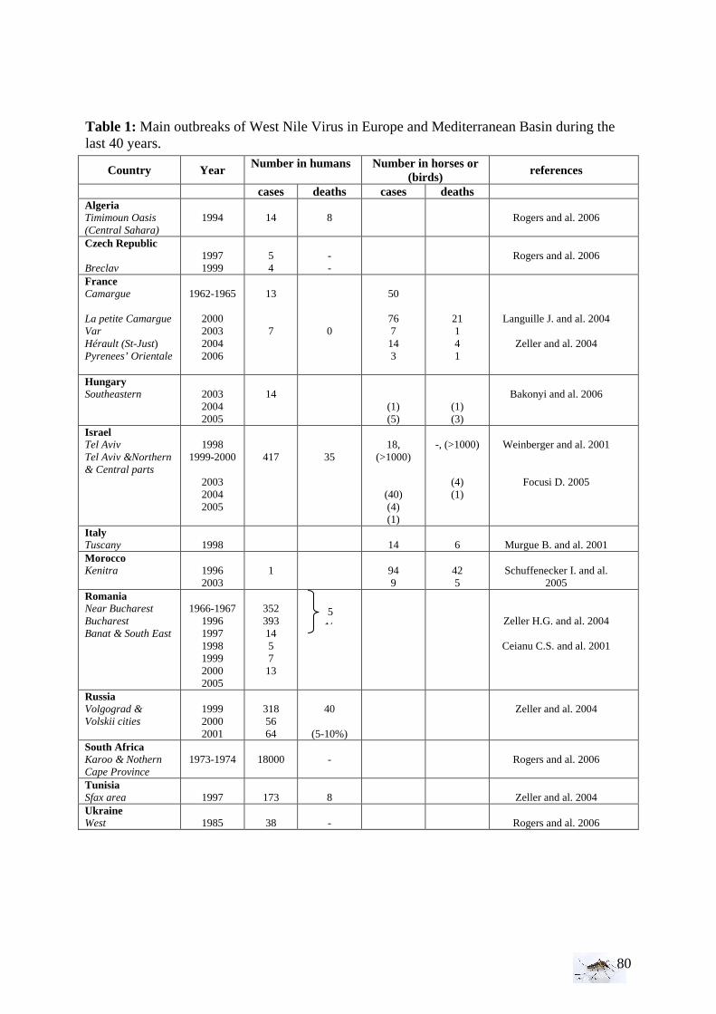
80

Table 1: Main outbreaks of West Nile Virus in Europe and Mediterranean Basin during the last 40 years.

Country Year Number in humans

Number in horses or (birds) references

cases deaths cases deaths Algeria Timimoun Oasis (Central Sahara)

1994

14

8

Rogers and al. 2006

Czech Republic Breclav

1997 1999

5 4

- -

Rogers and al. 2006

France Camargue La petite Camargue Var Hérault (St-Just) Pyrenees’ Orientale

1962-1965

2000 2003 2004 2006

13 7

0

50

76 7 14 3

21 1 4 1

Languille J. and al. 2004

Zeller and al. 2004

Hungary Southeastern

2003 2004 2005

14

(1) (5)

(1) (3)

Bakonyi and al. 2006

Israel Tel Aviv Tel Aviv &Northern & Central parts

1998

1999-2000

2003 2004 2005

417

35

18,

(>1000)

(40) (4) (1)

-, (>1000)

(4) (1)

Weinberger and al. 2001

Focusi D. 2005

Italy Tuscany

1998

14

6

Murgue B. and al. 2001

Morocco Kenitra

1996 2003

1

94 9

42 5

Schuffenecker I. and al.

2005 Romania Near Bucharest Bucharest Banat & South East

1966-1967

1996 1997 1998 1999 2000 2005

352 393 14 5 7 13

-

17

Zeller H.G. and al. 2004

Ceianu C.S. and al. 2001

Russia Volgograd & Volskii cities

1999 2000 2001

318 56 64

40

(5-10%)

Zeller and al. 2004

South Africa Karoo & Nothern Cape Province

1973-1974

18000

-

Rogers and al. 2006

Tunisia Sfax area

1997

173

8

Zeller and al. 2004

Ukraine West

1985

38

-

Rogers and al. 2006

5

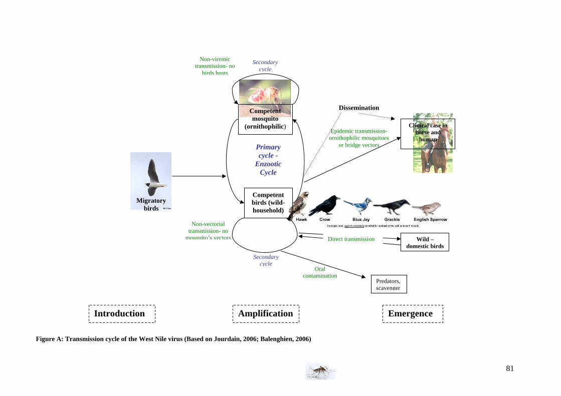
81

Figure A: Transmission cycle of the West Nile virus (Based on Jourdain, 2006; Balenghien, 2006)

Oral contamination

Epidemic transmission- ornithophilic mosquitoes

or bridge vectors

Dissemination

Non-vectorial transmission- no

mosquito’s vectors

Non-viremic transmission- no

birds hosts

Secondary cycle

Competent mosquito

(ornithophilic )

Competent birds (wild- household)

Primary cycle -

Enzootic Cycle

Secondary cycle

Introduction Amplification Emergence

Migratory birds

Clinical case in horse and

human

Predators, scavenger

Wild – domestic birds

Direct transmission

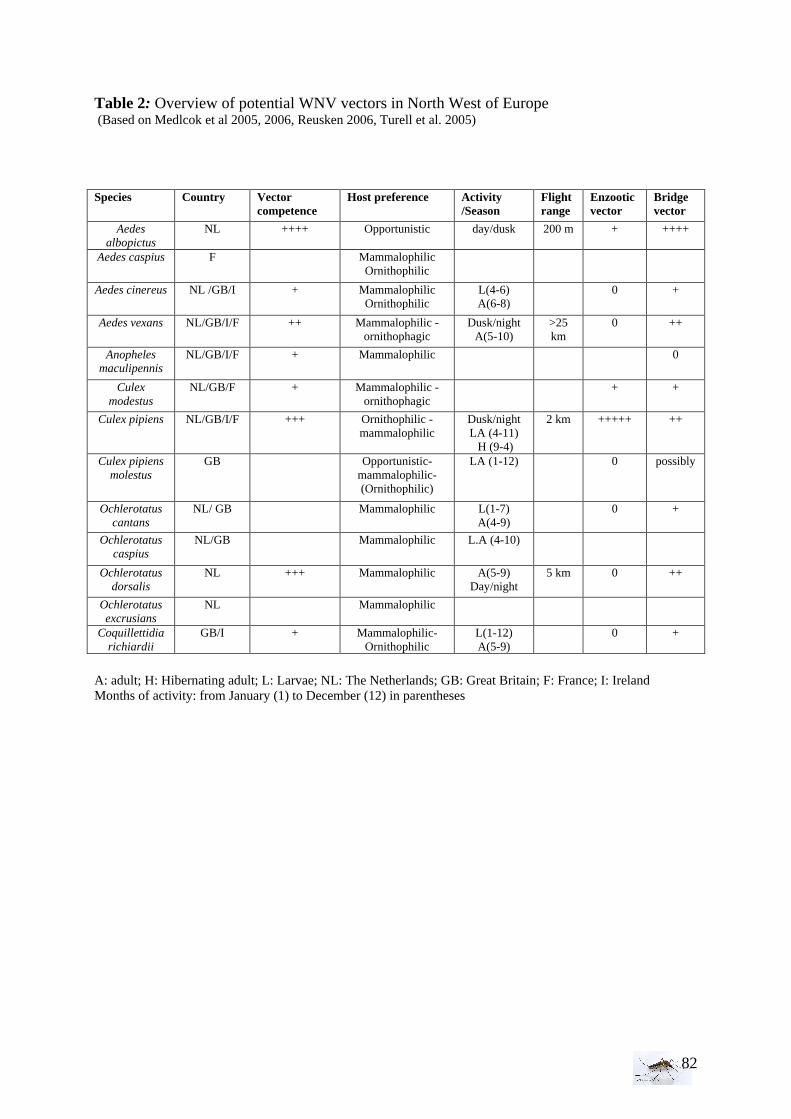
82

Table 2: Overview of potential WNV vectors in North West of Europe (Based on Medlcok et al 2005, 2006, Reusken 2006, Turell et al. 2005)

A: adult; H: Hibernating adult; L: Larvae; NL: The Netherlands; GB: Great Britain; F: France; I: Ireland Months of activity: from January (1) to December (12) in parentheses

Species Country Vector competence

Host preference Activity /Season

Flight range

Enzootic vector

Bridge vector

Aedes albopictus

NL ++++ Opportunistic day/dusk 200 m + ++++

Aedes caspius F Mammalophilic Ornithophilic

Aedes cinereus NL /GB/I + Mammalophilic Ornithophilic

L(4-6) A(6-8)

0 +

Aedes vexans NL/GB/I/F ++ Mammalophilic - ornithophagic

Dusk/night A(5-10)

>25 km

0 ++

Anopheles maculipennis

NL/GB/I/F + Mammalophilic 0

Culex modestus

NL/GB/F + Mammalophilic - ornithophagic

+ +

Culex pipiens NL/GB/I/F +++ Ornithophilic - mammalophilic

Dusk/night LA (4-11) H (9-4)

2 km +++++ ++

Culex pipiens molestus

GB Opportunistic- mammalophilic- (Ornithophilic)

LA (1-12) 0 possibly

Ochlerotatus cantans

NL/ GB Mammalophilic L(1-7) A(4-9)

0 +

Ochlerotatus caspius

NL/GB Mammalophilic L.A (4-10)

Ochlerotatus dorsalis

NL +++ Mammalophilic A(5-9) Day/night

5 km 0 ++

Ochlerotatus excrusians

NL Mammalophilic

Coquillettidia richiardii

GB/I + Mammalophilic- Ornithophilic

L(1-12) A(5-9)

0 +

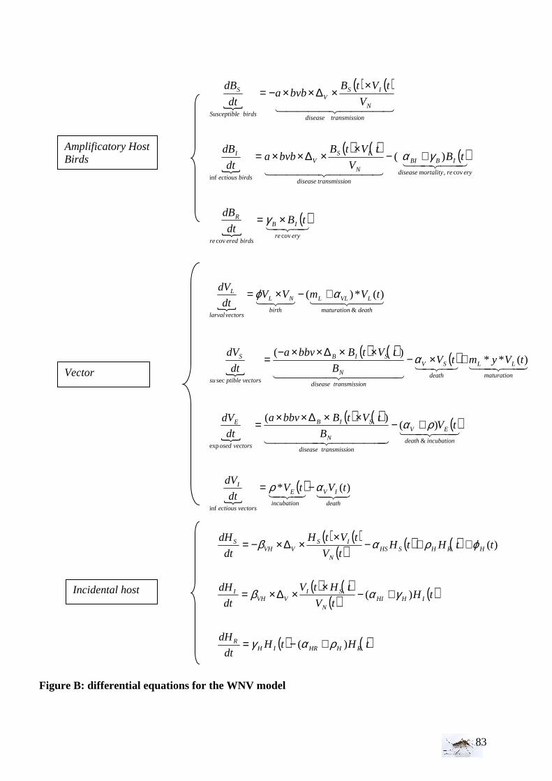
83

Figure B: differential equations for the WNV model

{

{

( ) ( ) ( )

{

( ) ( ) ( )

{( )

4342143421

443442144444 344444 21

44344214342144444 344444 21

44 344 2143421

death

IV

incubation

E

vectorsectious

I

incubationdeath

EV

ontransmissidisease

N

SIB

vectorsosed

E

maturation

LL

death

SV

ontransmissidisease

N

SIB

vectorsptiblesu

S

deathmaturation

LVLL

birth

NL

vectorslarval

L

tVtVdt

dV

tVB

tVtBbbva

dt

dV

tVymtVB

tVtBbbva

dt

dV

tVmVVdt

dV

)(*

)()(

)(**)(

)(*)(

inf

&exp

sec

&

αρ

ρα

α

αϕ

−=

+−××∆××

=

+×−××∆××−

=

+−×=

{

( ) ( )

{

( ) ( ) ( )

{( )

43421

44 344 214444 34444 21

4444 34444 21

eryre

IB

birdseredre

R

eryremortalitydisease

IBBI

ontransmissidisease

N

ISV

birdsectious

I

ontransmissidisease

N

ISV

birdseSusceptibl

S

tBdt

dB

tBV

tVtBbvba

dt

dB

V

tVtBbvba

dt

dB

covcov

cov,inf

)(

×=

+−×

×∆××=

××∆××−=

γ

γα

( ) ( )( ) ( ) ( )

( ) ( )( ) ( )

( ) ( )tHtHdt

dH

tHtV

tHtV

dt

dH

ttHtHtV

tVtH

dt

dH

RHHRIHR

IHHIN

SIVVH

I

HRHSHSN

ISVVH

S

)(

)(

)(

ραγ

γαβ

ϕραβ

+−=

+−×

×∆×=

++−×

×∆×−=

Incidental host

Vector

Amplificatory Host Birds

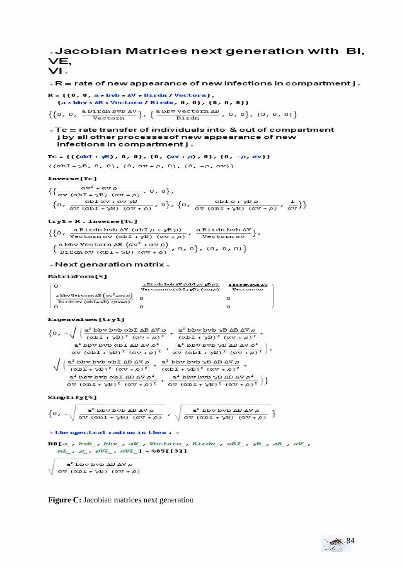
84

Figure C: Jacobian matrices next generation

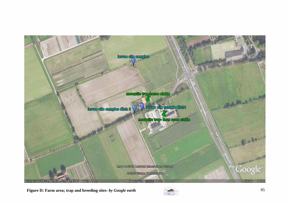
85

Figure D: Farm area; trap and breeding sites- by Google earth

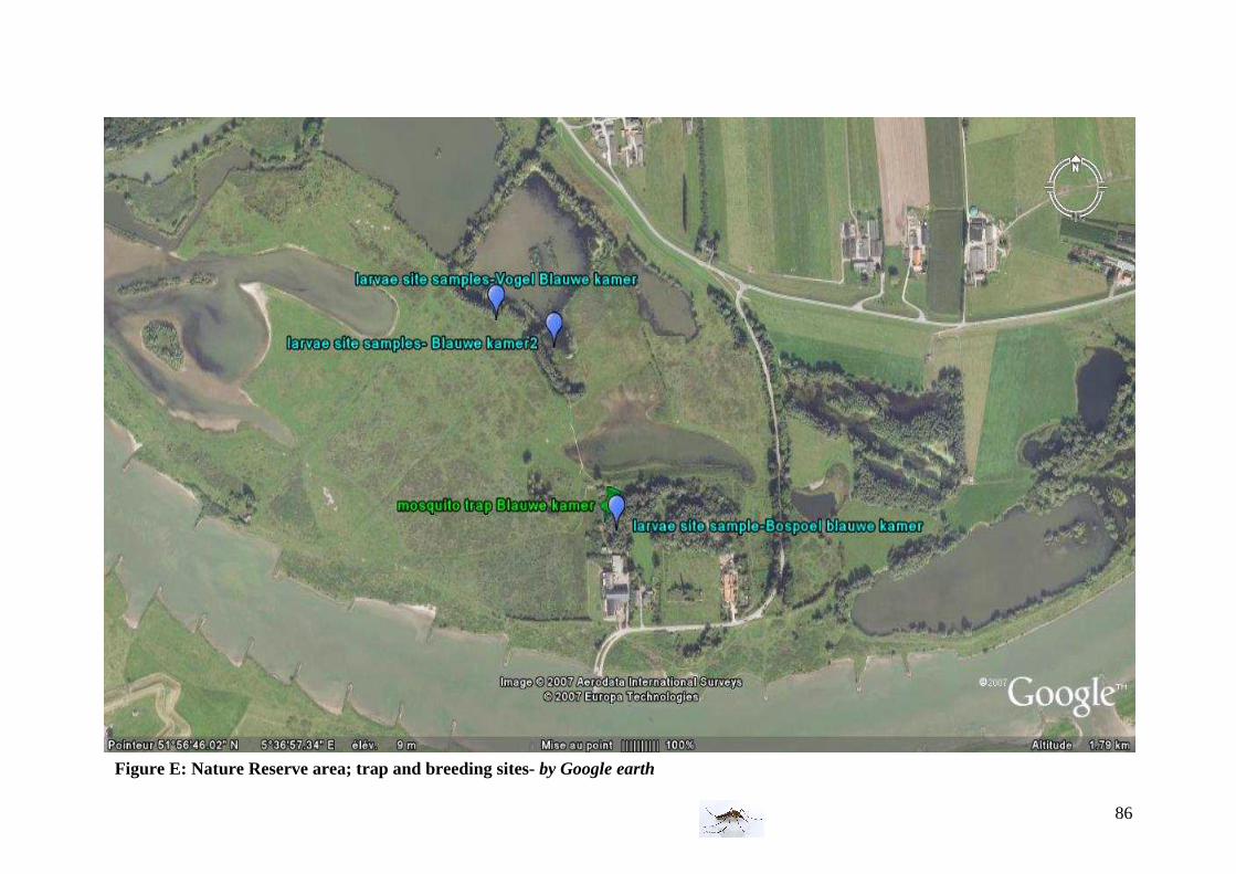
86

Figure E: Nature Reserve area; trap and breeding sites- by Google earth

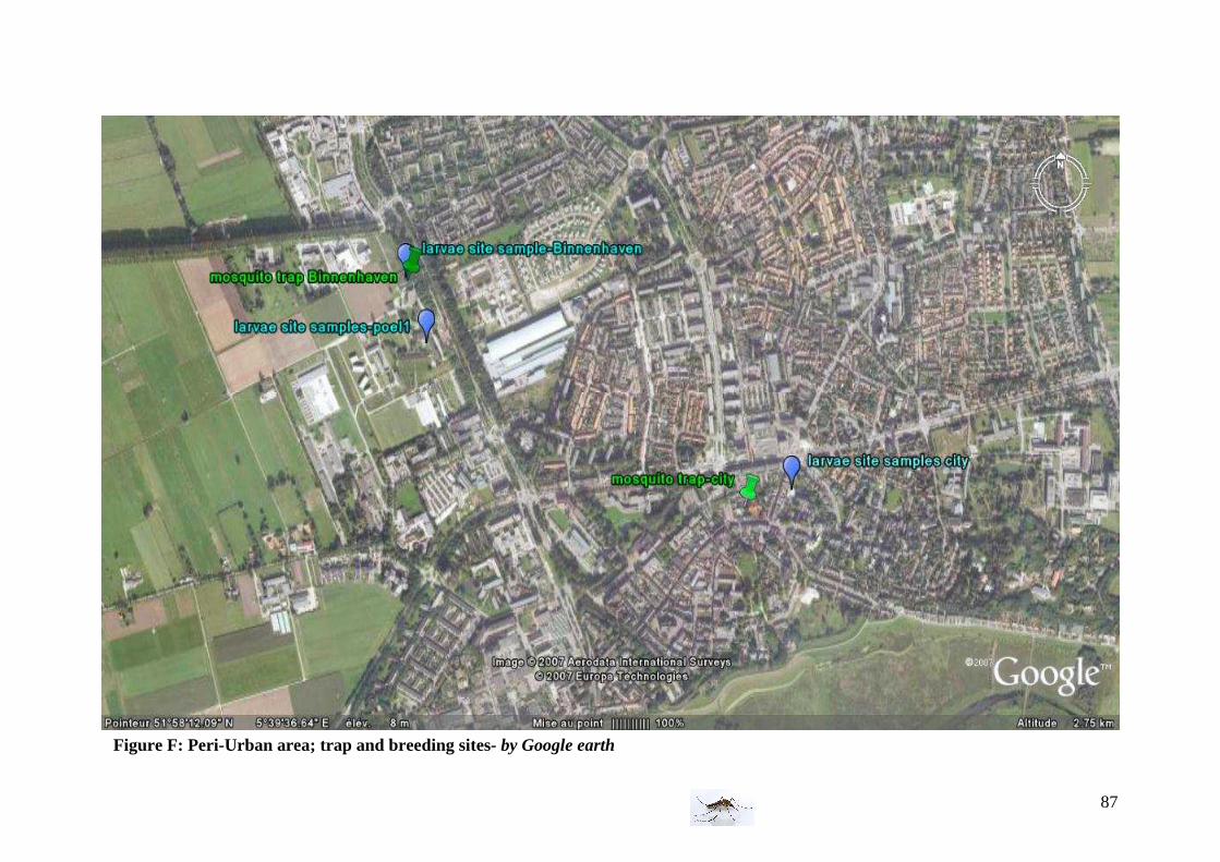
87

Figure F: Peri-Urban area; trap and breeding sites- by Google earth

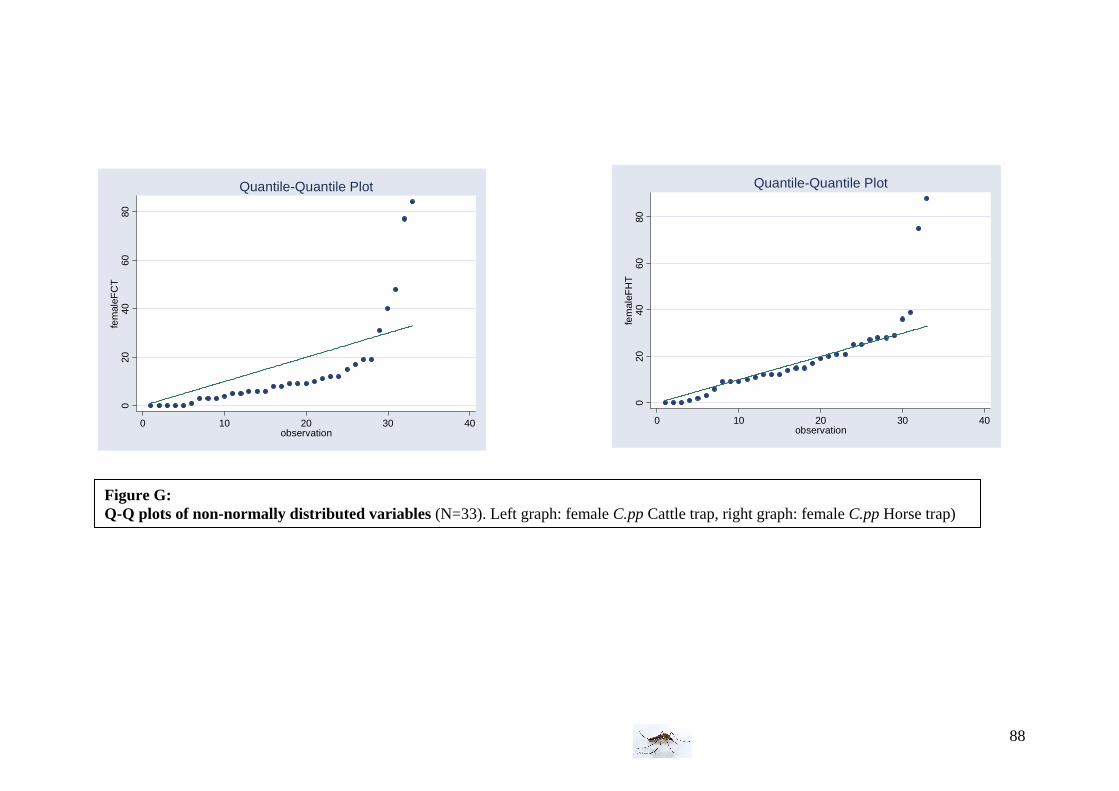
88

020

4060

80fe

mal

eFH

T

0 10 20 30 40observation

Quantile-Quantile Plot

020

4060

80fe

mal

eFC

T

0 10 20 30 40observation

Quantile-Quantile Plot

Figure G: Q-Q plots of non-normally distributed variables (N=33). Left graph: female C.pp Cattle trap, right graph: female C.pp Horse trap)

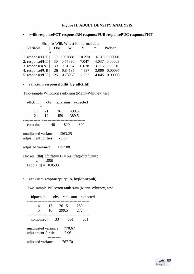
89

Figure H: ADULT DENSITY ANALYSIS • swilk responseFCT responseRN responsePUB responsePUC responseFHT Shapiro-Wilk W test for normal data Variable | Obs W V z Prob>z --------------------+------------------------------------------------- 1. responseFCT | 30 0.67688 10.270 4.816 0.00000 2. responseFHT | 30 0.77830 7.047 4.037 0.00003 3. responseRN | 30 0.81034 6.028 3.715 0.00010 4. responsePUB | 26 0.84135 4.537 3.099 0.00097 5. responsePUC | 25 0.73969 7.233 4.045 0.00003 • ranksum responsefctfht, by(idfctfht) Two-sample Wilcoxon rank-sum (Mann-Whitney) test idfctfht | obs rank sum expected -------------+--------------------------------- 1 | 21 361 430.5 2 | 19 459 389.5 -------------+--------------------------------- combined | 40 820 820 unadjusted variance 1363.25 adjustment for ties -5.37 ---------- adjusted variance 1357.88 Ho: res~tfht(idfctfht==1) = res~tfht(idfctfht==2) z = -1.886

Prob > |z| = 0.0593

• ranksum responsepucpub, by(idpucpub) Two-sample Wilcoxon rank-sum (Mann-Whitney) test idpucpub | obs rank sum expected -------------+--------------------------------- 4 | 17 261.5 289 5 | 16 299.5 272 -------------+--------------------------------- combined | 33 561 561 unadjusted variance 770.67 adjustment for ties -2.96 ---------- adjusted variance 767.70

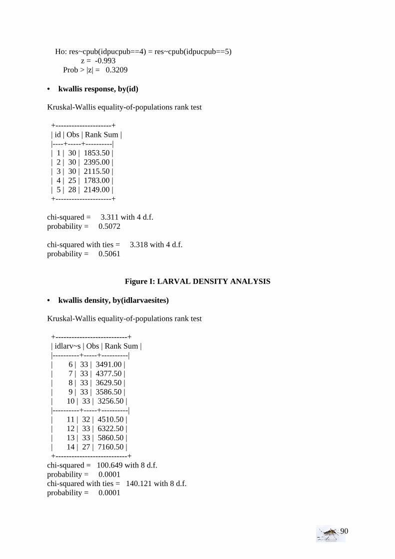
90

Ho: res~cpub(idpucpub==4) = res~cpub(idpucpub==5) z = -0.993 Prob > |z| = 0.3209

• kwallis response, by(id) Kruskal-Wallis equality-of-populations rank test +---------------------+ | id | Obs | Rank Sum | |----+-----+----------| | 1 | 30 | 1853.50 | | 2 | 30 | 2395.00 | | 3 | 30 | 2115.50 | | 4 | 25 | 1783.00 | | 5 | 28 | 2149.00 | +---------------------+ chi-squared = 3.311 with 4 d.f. probability = 0.5072 chi-squared with ties = 3.318 with 4 d.f. probability = 0.5061

Figure I: LARVAL DENSITY ANALYSIS • kwallis density, by(idlarvaesites) Kruskal-Wallis equality-of-populations rank test +---------------------------+ | idlarv~s | Obs | Rank Sum | |----------+-----+----------| | 6 | 33 | 3491.00 | | 7 | 33 | 4377.50 | | 8 | 33 | 3629.50 | | 9 | 33 | 3586.50 | | 10 | 33 | 3256.50 | |----------+-----+----------| | 11 | 32 | 4510.50 | | 12 | 33 | 6322.50 | | 13 | 33 | 5860.50 | | 14 | 27 | 7160.50 | +---------------------------+ chi-squared = 100.649 with 8 d.f. probability = 0.0001 chi-squared with ties = 140.121 with 8 d.f. probability = 0.0001

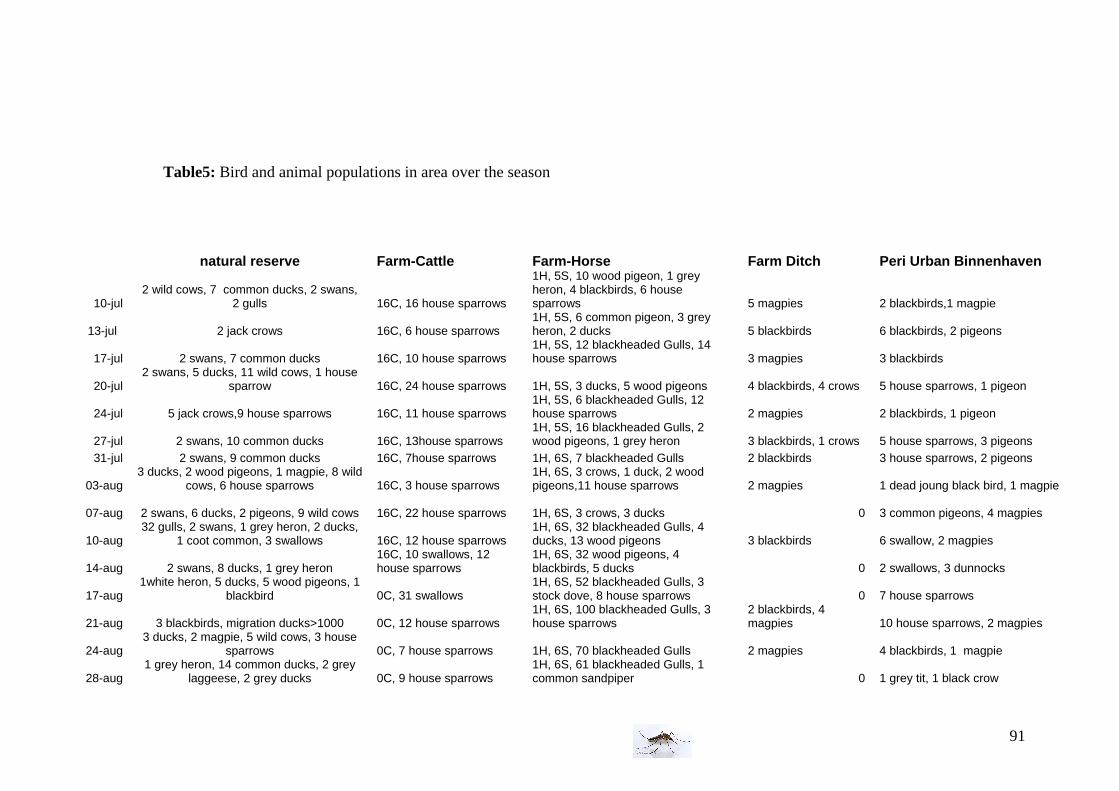
91

Table5: Bird and animal populations in area over the season

natural reserve Farm-Cattle Farm-Horse Farm Ditch Peri Urban Binnenhaven

10-jul 2 wild cows, 7 common ducks, 2 swans,

2 gulls 16C, 16 house sparrows

1H, 5S, 10 wood pigeon, 1 grey heron, 4 blackbirds, 6 house sparrows 5 magpies 2 blackbirds,1 magpie

13-jul 2 jack crows 16C, 6 house sparrows 1H, 5S, 6 common pigeon, 3 grey heron, 2 ducks 5 blackbirds 6 blackbirds, 2 pigeons

17-jul 2 swans, 7 common ducks 16C, 10 house sparrows 1H, 5S, 12 blackheaded Gulls, 14 house sparrows 3 magpies 3 blackbirds

20-jul 2 swans, 5 ducks, 11 wild cows, 1 house

sparrow 16C, 24 house sparrows 1H, 5S, 3 ducks, 5 wood pigeons 4 blackbirds, 4 crows 5 house sparrows, 1 pigeon

24-jul 5 jack crows,9 house sparrows 16C, 11 house sparrows 1H, 5S, 6 blackheaded Gulls, 12 house sparrows 2 magpies 2 blackbirds, 1 pigeon

27-jul 2 swans, 10 common ducks 16C, 13house sparrows 1H, 5S, 16 blackheaded Gulls, 2 wood pigeons, 1 grey heron 3 blackbirds, 1 crows 5 house sparrows, 3 pigeons

31-jul 2 swans, 9 common ducks 16C, 7house sparrows 1H, 6S, 7 blackheaded Gulls 2 blackbirds 3 house sparrows, 2 pigeons

03-aug 3 ducks, 2 wood pigeons, 1 magpie, 8 wild

cows, 6 house sparrows 16C, 3 house sparrows 1H, 6S, 3 crows, 1 duck, 2 wood pigeons,11 house sparrows 2 magpies 1 dead joung black bird, 1 magpie

07-aug 2 swans, 6 ducks, 2 pigeons, 9 wild cows 16C, 22 house sparrows 1H, 6S, 3 crows, 3 ducks 0 3 common pigeons, 4 magpies

10-aug 32 gulls, 2 swans, 1 grey heron, 2 ducks,

1 coot common, 3 swallows 16C, 12 house sparrows 1H, 6S, 32 blackheaded Gulls, 4 ducks, 13 wood pigeons 3 blackbirds 6 swallow, 2 magpies

14-aug 2 swans, 8 ducks, 1 grey heron 16C, 10 swallows, 12 house sparrows

1H, 6S, 32 wood pigeons, 4 blackbirds, 5 ducks 0 2 swallows, 3 dunnocks

17-aug 1white heron, 5 ducks, 5 wood pigeons, 1

blackbird 0C, 31 swallows 1H, 6S, 52 blackheaded Gulls, 3 stock dove, 8 house sparrows 0 7 house sparrows

21-aug 3 blackbirds, migration ducks>1000 0C, 12 house sparrows 1H, 6S, 100 blackheaded Gulls, 3 house sparrows

2 blackbirds, 4 magpies 10 house sparrows, 2 magpies

24-aug 3 ducks, 2 magpie, 5 wild cows, 3 house

sparrows 0C, 7 house sparrows 1H, 6S, 70 blackheaded Gulls 2 magpies 4 blackbirds, 1 magpie

28-aug 1 grey heron, 14 common ducks, 2 grey

laggeese, 2 grey ducks 0C, 9 house sparrows 1H, 6S, 61 blackheaded Gulls, 1 common sandpiper 0 1 grey tit, 1 black crow

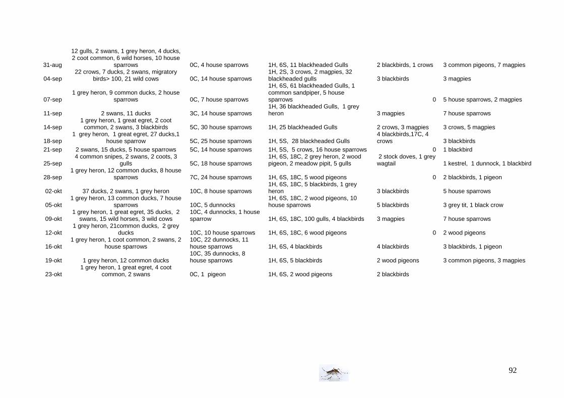
92

31-aug

12 gulls, 2 swans, 1 grey heron, 4 ducks, 2 coot common, 6 wild horses, 10 house

sparrows 0C, 4 house sparrows 1H, 6S, 11 blackheaded Gulls 2 blackbirds, 1 crows 3 common pigeons, 7 magpies

04-sep 22 crows, 7 ducks, 2 swans, migratory

birds> 100, 21 wild cows 0C, 14 house sparrows 1H, 2S, 3 crows, 2 magpies, 32 blackheaded gulls 3 blackbirds 3 magpies

07-sep 1 grey heron, 9 common ducks, 2 house

sparrows 0C, 7 house sparrows

1H, 6S, 61 blackheaded Gulls, 1 common sandpiper, 5 house sparrows 0 5 house sparrows, 2 magpies

11-sep 2 swans, 11 ducks 3C, 14 house sparrows 1H, 36 blackheaded Gulls, 1 grey heron 3 magpies 7 house sparrows

14-sep 1 grey heron, 1 great egret, 2 coot

common, 2 swans, 3 blackbirds 5C, 30 house sparrows 1H, 25 blackheaded Gulls 2 crows, 3 magpies 3 crows, 5 magpies

18-sep 1 grey heron, 1 great egret, 27 ducks,1

house sparrow 5C, 25 house sparrows 1H, 5S, 28 blackheaded Gulls 4 blackbirds,17C, 4 crows 3 blackbirds

21-sep 2 swans, 15 ducks, 5 house sparrows 5C, 14 house sparrows 1H, 5S, 5 crows, 16 house sparrows 0 1 blackbird

25-sep 4 common snipes, 2 swans, 2 coots, 3

gulls 5C, 18 house sparrows 1H, 6S, 18C, 2 grey heron, 2 wood pigeon, 2 meadow pipit, 5 gulls

2 stock doves, 1 grey wagtail 1 kestrel, 1 dunnock, 1 blackbird

28-sep 1 grey heron, 12 common ducks, 8 house

sparrows 7C, 24 house sparrows 1H, 6S, 18C, 5 wood pigeons 0 2 blackbirds, 1 pigeon

02-okt 37 ducks, 2 swans, 1 grey heron 10C, 8 house sparrows 1H, 6S, 18C, 5 blackbirds, 1 grey heron 3 blackbirds 5 house sparrows

05-okt 1 grey heron, 13 common ducks, 7 house

sparrows 10C, 5 dunnocks 1H, 6S, 18C, 2 wood pigeons, 10 house sparrows 5 blackbirds 3 grey tit, 1 black crow

09-okt 1 grey heron, 1 great egret, 35 ducks, 2

swans, 15 wild horses, 3 wild cows 10C, 4 dunnocks, 1 house sparrow 1H, 6S, 18C, 100 gulls, 4 blackbirds 3 magpies 7 house sparrows

12-okt 1 grey heron, 21common ducks, 2 grey

ducks 10C, 10 house sparrows 1H, 6S, 18C, 6 wood pigeons 0 2 wood pigeons

16-okt 1 grey heron, 1 coot common, 2 swans, 2

house sparrows 10C, 22 dunnocks, 11 house sparrows 1H, 6S, 4 blackbirds 4 blackbirds 3 blackbirds, 1 pigeon

19-okt 1 grey heron, 12 common ducks 10C, 35 dunnocks, 8 house sparrows 1H, 6S, 5 blackbirds 2 wood pigeons 3 common pigeons, 3 magpies

23-okt 1 grey heron, 1 great egret, 4 coot

common, 2 swans 0C, 1 pigeon 1H, 6S, 2 wood pigeons 2 blackbirds

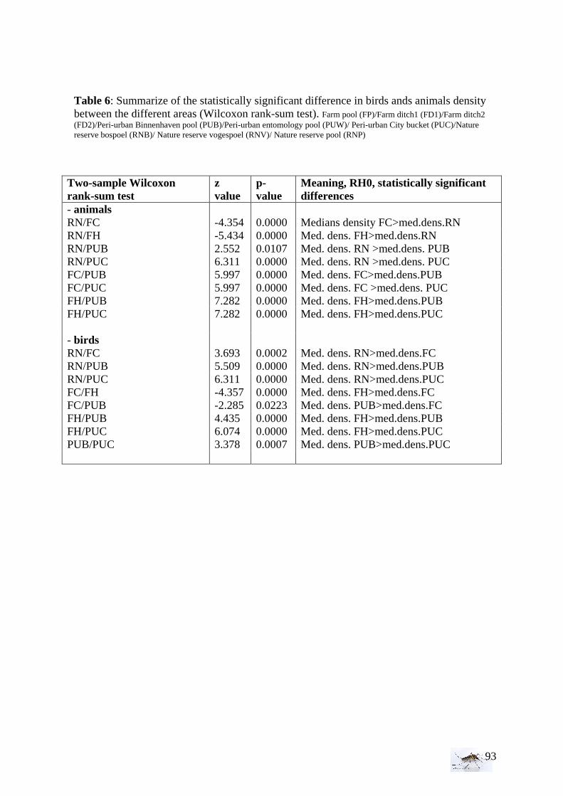
93

Two-sample Wilcoxon rank-sum test

z value

p-value

Meaning, RH0, statistically significant differences

- animals RN/FC

-4.354

0.0000

Medians density FC>med.dens.RN

RN/FH -5.434 0.0000 Med. dens. FH>med.dens.RN RN/PUB 2.552 0.0107 Med. dens. RN >med.dens. PUB RN/PUC 6.311 0.0000 Med. dens. RN >med.dens. PUC FC/PUB 5.997 0.0000 Med. dens. FC>med.dens.PUB FC/PUC 5.997 0.0000 Med. dens. FC >med.dens. PUC FH/PUB 7.282 0.0000 Med. dens. FH>med.dens.PUB FH/PUC 7.282 0.0000 Med. dens. FH>med.dens.PUC

- birds RN/FC

3.693

0.0002

Med. dens. RN>med.dens.FC

RN/PUB 5.509 0.0000 Med. dens. RN>med.dens.PUB RN/PUC 6.311 0.0000 Med. dens. RN>med.dens.PUC FC/FH -4.357 0.0000 Med. dens. FH>med.dens.FC FC/PUB -2.285 0.0223 Med. dens. PUB>med.dens.FC FH/PUB 4.435 0.0000 Med. dens. FH>med.dens.PUB FH/PUC 6.074 0.0000 Med. dens. FH>med.dens.PUC PUB/PUC 3.378 0.0007 Med. dens. PUB>med.dens.PUC

Table 6: Summarize of the statistically significant difference in birds ands animals density between the different areas (Wilcoxon rank-sum test). Farm pool (FP)/Farm ditch1 (FD1)/Farm ditch2 (FD2)/Peri-urban Binnenhaven pool (PUB)/Peri-urban entomology pool (PUW)/ Peri-urban City bucket (PUC)/Nature reserve bospoel (RNB)/ Nature reserve vogespoel (RNV)/ Nature reserve pool (RNP)

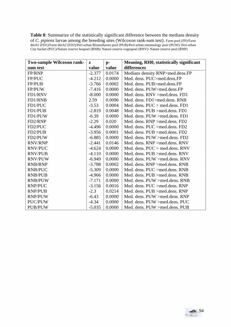
94

Two-sample Wilcoxon rank-sum test

z value

p-value

Meaning, RH0, statistically significant differences

FP/RNP -2.377 0.0174 Medians density RNP>med.dens.FP FP/PUC -4.212 0.0000 Med. dens. PUC>med.dens.FP FP/PUB -3.766 0.0002 Med. dens. PUB>med.dens.FP FP/PUW -7.416 0.0000 Med. dens. PUW>med.dens.FP FD1/RNV -8.000 0.0000 Med. dens. RNV >med.dens. FD1 FD1/RNB 2.59 0.0096 Med. dens. FD1>med.dens. RNB FD1/PUC -3.53 0.0004 Med. dens. PUC > med.dens. FD1 FD1/PUB -2.819 0.0048 Med. dens. PUB >med.dens. FD1 FD1/PUW -6.39 0.0000 Med. dens. PUW >med.dens. FD1 FD2/RNP -2.29 0.020 Med. dens. RNP >med.dens. FD2 FD2/PUC -4.496 0.0000 Med. dens. PUC >med.dens. FD2 FD2/PUB -3.956 0.0001 Med. dens. PUB >med.dens. FD2 FD2/PUW -6.885 0.0000 Med. dens. PUW >med.dens. FD2 RNV/RNP -2.441 0.0146 Med. dens. RNP >med.dens. RNV RNV/PUC -4.624 0.0000 Med. dens. PUC > med.dens. RNV RNV/PUB -4.110 0.0000 Med. dens. PUB >med.dens. RNV RNV/PUW -6.949 0.0000 Med. dens. PUW >med.dens. RNV RNB/RNP -3.788 0.0002 Med. dens. RNP >med.dens. RNB RNB/PUC -5.309 0.0000 Med. dens. PUC >med.dens. RNB RNB/PUB -4.966 0.0000 Med. dens. PUB >med.dens. RNB RNB/PUW -7.171 0.0000 Med. dens. PUW >med.dens. RNB RNP/PUC -3.156 0.0016 Med. dens. PUC >med.dens. RNP RNP/PUB -2.3 0.0214 Med. dens. PUB >med.dens. RNP RNP/PUW -6.43 0.0000 Med. dens. PUW >med.dens. RNP PUC/PUW -4.34 0.0000 Med. dens. PUW >med.dens. PUC PUB/PUW -5.035 0.0000 Med. dens. PUW >med.dens. PUB

Table 8: Summarize of the statistically significant difference between the medians density of C. pipiens larvae among the breeding sites (Wilcoxon rank-sum test). Farm pool (FP)/Farm ditch1 (FD1)/Farm ditch2 (FD2)/Peri-urban Binnenhaven pool (PUB)/Peri-urban entomology pool (PUW)/ Peri-urban City bucket (PUC)/Nature reserve bospoel (RNB)/ Nature reserve vogespoel (RNV)/ Nature reserve pool (RNP)

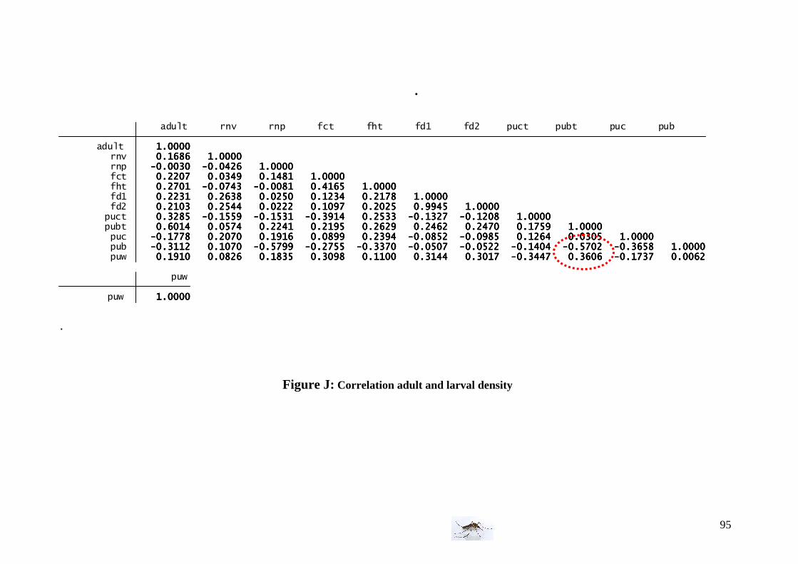
95

.

.

puw 1111....0000000000000000 puw

puw 0000....1111999911110000 0000....0000888822226666 0000....1111888833335555 0000....3333000099998888 0000....1111111100000000 0000....3333111144444444 0000....3333000011117777 ----0000....3333444444447777 0000....3333666600006666 ----0000....1111777733337777 0000....0000000066662222 pub ----0000....3333111111112222 0000....1111000077770000 ----0000....5555777799999999 ----0000....2222777755555555 ----0000....3333333377770000 ----0000....0000555500007777 ----0000....0000555522222222 ----0000....1111444400004444 ----0000....5555777700002222 ----0000....3333666655558888 1111....0000000000000000 puc ----0000....1111777777778888 0000....2222000077770000 0000....1111999911116666 0000....0000888899999999 0000....2222333399994444 ----0000....0000888855552222 ----0000....0000999988885555 0000....1111222266664444 0000....0000333300005555 1111....0000000000000000 pubt 0000....6666000011114444 0000....0000555577774444 0000....2222222244441111 0000....2222111199995555 0000....2222666622229999 0000....2222444466662222 0000....2222444477770000 0000....1111777755559999 1111....0000000000000000 puct 0000....3333222288885555 ----0000....1111555555559999 ----0000....1111555533331111 ----0000....3333999911114444 0000....2222555533333333 ----0000....1111333322227777 ----0000....1111222200008888 1111....0000000000000000 fd2 0000....2222111100003333 0000....2222555544444444 0000....0000222222222222 0000....1111000099997777 0000....2222000022225555 0000....9999999944445555 1111....0000000000000000 fd1 0000....2222222233331111 0000....2222666633338888 0000....0000222255550000 0000....1111222233334444 0000....2222111177778888 1111....0000000000000000 fht 0000....2222777700001111 ----0000....0000777744443333 ----0000....0000000088881111 0000....4444111166665555 1111....0000000000000000 fct 0000....2222222200007777 0000....0000333344449999 0000....1111444488881111 1111....0000000000000000 rnp ----0000....0000000033330000 ----0000....0000444422226666 1111....0000000000000000 rnv 0000....1111666688886666 1111....0000000000000000 adult 1111....0000000000000000 adult rnv rnp fct fht fd1 fd2 puct pubt puc pub

Figure J: Correlation adult and larval density

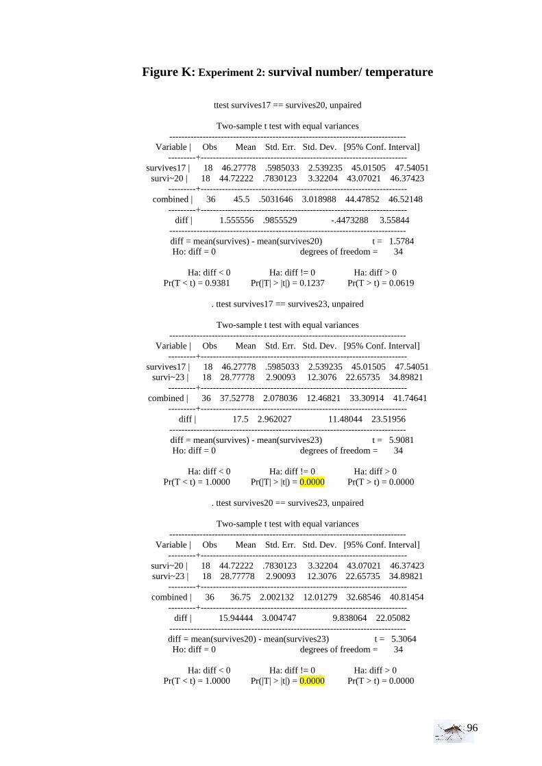
96

Figure K: Experiment 2: survival number/ temperature

ttest survives17 == survives20, unpaired

Two-sample t test with equal variances ------------------------------------------------------------------------------

Variable | Obs Mean Std. Err. Std. Dev. [95% Conf. Interval] ---------+--------------------------------------------------------------------

survives17 | 18 46.27778 .5985033 2.539235 45.01505 47.54051 survi~20 | 18 44.72222 .7830123 3.32204 43.07021 46.37423

---------+-------------------------------------------------------------------- combined | 36 45.5 .5031646 3.018988 44.47852 46.52148

---------+-------------------------------------------------------------------- diff | 1.555556 .9855529 -.4473288 3.55844 ------------------------------------------------------------------------------

diff = mean(survives) - mean(survives20) t = 1.5784 Ho: diff = 0 degrees of freedom = 34

Ha: diff < 0 Ha: diff != 0 Ha: diff > 0

Pr(T < t) = 0.9381 Pr(|T| > |t|) = 0.1237 Pr(T > t) = 0.0619

. ttest survives17 == survives23, unpaired



survives17 | 18 46.27778 .5985033 2.539235 45.01505 47.54051 survi~23 | 18 28.77778 2.90093 12.3076 22.65735 34.89821

---------+-------------------------------------------------------------------- combined | 36 37.52778 2.078036 12.46821 33.30914 41.74641

---------+-------------------------------------------------------------------- diff | 17.5 2.962027 11.48044 23.51956 ------------------------------------------------------------------------------

diff = mean(survives) - mean(survives23) t = 5.9081 Ho: diff = 0 degrees of freedom = 34


Pr(T < t) = 1.0000 Pr(|T| > |t|) = 0.0000 Pr(T > t) = 0.0000

. ttest survives20 == survives23, unpaired



survi~20 | 18 44.72222 .7830123 3.32204 43.07021 46.37423 survi~23 | 18 28.77778 2.90093 12.3076 22.65735 34.89821

---------+-------------------------------------------------------------------- combined | 36 36.75 2.002132 12.01279 32.68546 40.81454

---------+-------------------------------------------------------------------- diff | 15.94444 3.004747 9.838064 22.05082 ------------------------------------------------------------------------------

diff = mean(survives20) - mean(survives23) t = 5.3064 Ho: diff = 0 degrees of freedom = 34


Pr(T < t) = 1.0000 Pr(|T| > |t|) = 0.0000 Pr(T > t) = 0.0000

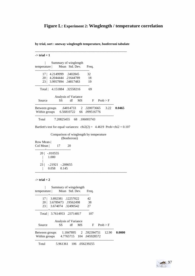
97

Figure L: Experiment 2: Winglength / temperature correlation by trial, sort : oneway winglength temperature, bonferroni tabulate ------------------------------------------------------------------------------------ -> trial = 1

| Summary of winglength temperature | Mean Std. Dev. Freq. ------------+------------------------------------ 17 | 4.2149999 .3402845 32 20 | 4.2044444 .21644789 18 23 | 3.9957894 .34817483 19 ------------+------------------------------------ Total | 4.151884 .32558216 69 Analysis of Variance Source SS df MS F Prob > F ------------------------------------------------------------------------ Between groups .64014733 2 .320073665 3.22 0.0465 Within groups 6.56810722 66 .099516776 ------------------------------------------------------------------------ Total 7.20825455 68 .106003743 Bartlett's test for equal variances: chi2(2) = 4.4619 Prob>chi2 = 0.107 Comparison of winglength by temperature (Bonferroni) Row Mean-| Col Mean | 17 20 ---------+---------------------- 20 | -.010555 | 1.000 | 23 | -.21921 -.208655 | 0.058 0.145 ------------------------------------------------------------------------------------ -> trial = 2 | Summary of wingslength temperature | Mean Std. Dev. Freq. ------------+------------------------------------ 17 | 3.892381 .12257022 42 20 | 3.6789473 .19562498 38 23 | 3.674074 .32490542 27 ------------+------------------------------------ Total | 3.7614953 .23714817 107 Analysis of Variance Source SS df MS F Prob > F ------------------------------------------------------------------------ Between groups 1.1847895 2 .592394751 12.90 0.0000 Within groups 4.7765715 104 .045928572 ------------------------------------------------------------------------ Total 5.961361 106 .056239255

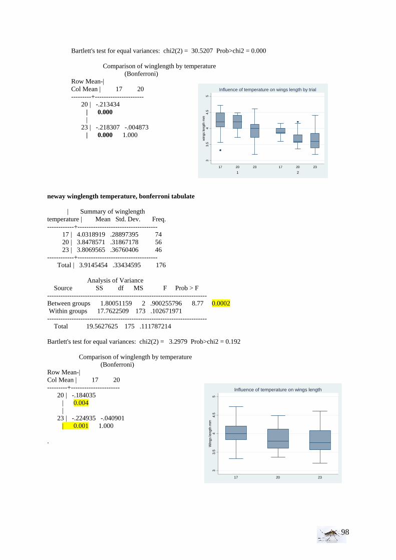
98

33.

54

4.5

5W

ings

leng

th m

m

17 20 23

Influence of temperature on wings length

33.

54

4.5

5w

ings

leng

th m

m

1 2

17 20 23 17 20 23

Influence of temperature on wings length by trial

Bartlett's test for equal variances: chi2(2) = 30.5207 Prob>chi2 = 0.000 Comparison of winglength by temperature (Bonferroni) Row Mean-| Col Mean | 17 20 ---------+---------------------- 20 | -.213434 | 0.000 | 23 | -.218307 -.004873 | 0.000 1.000

neway winglength temperature, bonferroni tabulate | Summary of winglength temperature | Mean Std. Dev. Freq. ------------+------------------------------------ 17 | 4.0318919 .28897395 74 20 | 3.8478571 .31867178 56 23 | 3.8069565 .36760406 46 ------------+------------------------------------ Total | 3.9145454 .33434595 176 Analysis of Variance Source SS df MS F Prob > F ------------------------------------------------------------------------ Between groups 1.80051159 2 .900255796 8.77 0.0002 Within groups 17.7622509 173 .102671971 ------------------------------------------------------------------------ Total 19.5627625 175 .111787214 Bartlett's test for equal variances: chi2(2) = 3.2979 Prob>chi2 = 0.192 Comparison of winglength by temperature (Bonferroni) Row Mean-| Col Mean | 17 20 ---------+---------------------- 20 | -.184035 | 0.004 | 23 | -.224935 -.040901 | 0.001 1.000 .

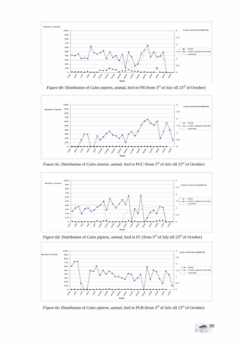
99

0

100

200

300

400

500

600

700

800

900

1000

03-ju

l

10-ju

l

17-ju

l

24-ju

l

31-ju

l

07-aug

14-aug

21-aug

28-aug

04-sep

11-sep

18-sep

25-sep

02-okt

09-okt

16-okt

23-okt

Date

Number of birds

0

0.5

1

1.5

2

2.5

3

C.pp & animals [log(N+1)]

birds


animals

Figure 6d: Distribution of Culex pipiens, animal, bird in FC (from 3rd of July till 23rd of October)

0

100

200

300

400

500

600

700

800

900

1000

03-ju

l

10-ju

l

17-ju

l

24-ju

l

31-ju

l

07-a

ug

14-a

ug

21-a

ug

28-a

ug

04-sep

11-sep

18-sep

25-sep

02-o

kt

09-o

kt

16-o

kt

23-o

kt

Date

Number of birds

0

0.5

1

1.5

2

2.5

3 C.pp & animals [log(N=1)]

birds


animals

Figure 6b: Distribution of Culex pipiens, animal, bird in FH (from 3rd of July till 23rd of October)

0

100

200

300

400

500

600

700

800

900

1000

03-ju

l

10-ju

l

17-ju

l

24-ju

l

31-ju

l

07-a

ug

14-a

ug

21-a

ug

28-a

ug

04-sep

11-sep

18-sep

25-sep

02-o

kt

09-o

kt

16-o

kt

23-o

kt

Date

Number of birds

0

0.5

1

1.5

2

2.5

3C.pp & animals [log(N+1)]

birds


animals

Figure 6e: Distribution of Culex pipiens, animal, bird in PUB (from 3rd of July till 23rd of October)

Figure 6c: Distribution of Culex pipiens, animal, bird in PUC (from 3rd of July till 23rd of October)

0

100

200

300

400

500

600

700

800

900

1000

03-ju

l

10-ju

l

17-ju

l

24-ju

l

31-ju

l

07-a

ug

14-a

ug

21-a

ug

28-a

ug

04-s

ep

11-s

ep

18-s

ep

25-s

ep

02-o

kt

09-o

kt

16-o

kt

23-o

kt

Date

Number of birds

0

0.5

1

1.5

2

2.5

3 C.pp & animals [log(N+1)]

birds


animals

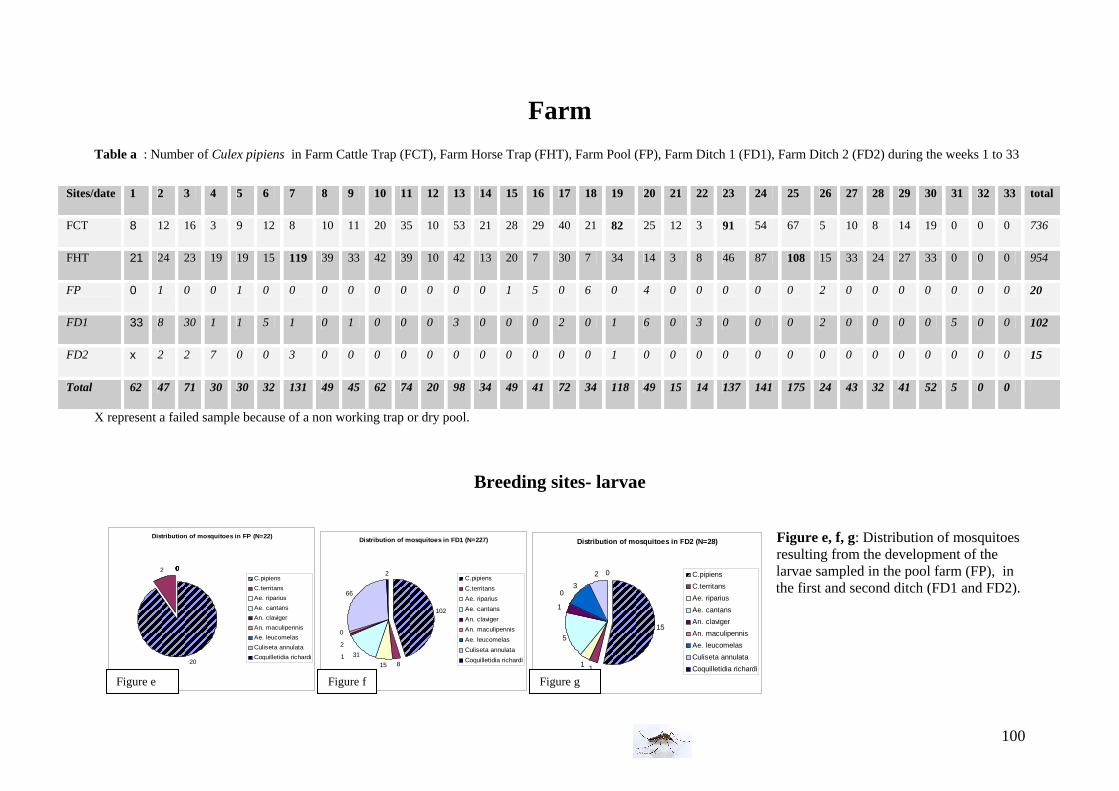
100

Farm

Table a : Number of Culex pipiens in Farm Cattle Trap (FCT), Farm Horse Trap (FHT), Farm Pool (FP), Farm Ditch 1 (FD1), Farm Ditch 2 (FD2) during the weeks 1 to 33

X represent a failed sample because of a non working trap or dry pool.

Breeding sites- larvae

Figure e, f, g: Distribution of mosquitoes resulting from the development of the larvae sampled in the pool farm (FP), in the first and second ditch (FD1 and FD2).

Sites/date 1 2 3 4 5 6 7 8 9 10 11 12 13 14 15 16 17 18 19 20 21 22 23 24 25 26 27 28 29 30 31 32 33 total

FCT 8 12 16 3 9 12 8 10 11 20 35 10 53 21 28 29 40 21 82 25 12 3 91 54 67 5 10 8 14 19 0 0 0 736

FHT 21 24 23 19 19 15 119 39 33 42 39 10 42 13 20 7 30 7 34 14 3 8 46 87 108 15 33 24 27 33 0 0 0 954

FP 0 1 0 0 1 0 0 0 0 0 0 0 0 0 1 5 0 6 0 4 0 0 0 0 0 2 0 0 0 0 0 0 0 20

FD1 33 8 30 1 1 5 1 0 1 0 0 0 3 0 0 0 2 0 1 6 0 3 0 0 0 2 0 0 0 0 5 0 0 102

FD2 x 2 2 7 0 0 3 0 0 0 0 0 0 0 0 0 0 0 1 0 0 0 0 0 0 0 0 0 0 0 0 0 0 15

Total 62 47 71 30 30 32 131 49 45 62 74 20 98 34 49 41 72 34 118 49 15 14 137 141 175 24 43 32 41 52 5 0 0

Distribution of mosquitoes in FD1 (N=227)

102

815

311

2

0

66

2C.pipiens

C.territans

Ae. riparius

Ae. cantans

An. claviger

An. maculipennis

Ae. leucomelas

Culiseta annulata


Distribution of mosquitoes in FP (N=22)

00000002

20

C.pipiens

C.territans

Ae. riparius

Ae. cantans

An. claviger

An. maculipennis

Ae. leucomelas

Culiseta annulata


Distribution of mosquitoes in FD2 (N=28)

15

11

5

1

03

2 0 C.pipiens

C.territans

Ae. riparius

Ae. cantans

An. claviger

An. maculipennis

Ae. leucomelas

Culiseta annulata


Figure g Figure e Figure f

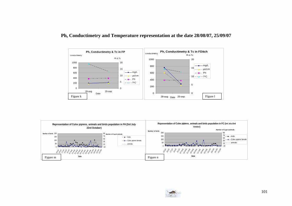
101

Representation of Culex pipiens, animals and birds population in FH (3rd July-23rd October)

0

50

100

150

200

03-ju

l10

-jul

17-ju

l24

-jul

31-ju

l07

-aug

14-a

ug21

-aug

28-a

ug04

-sep

11-s

ep18

-sep

25-s

ep02

-okt

09-o

kt16

-okt

23-o

kt

Date

Number of birds

-10

10

30

50

70

90 Number of C.pp & animals

birds


animals

Representation of Culex pipiens, animals and birds population in FC ( 3rd July-23rd

October )

0

50

100

150

200

03-ju

l10

-jul

17-ju

l24

-jul

31-ju

l07

-aug

14-a

ug21

-aug

28-a

ug04

-sep

11-s

ep18

-sep

25-s

ep02

-okt

09-o

kt16

-okt

23-o

kt

Date

Number of birds

-101030507090

Number of C.pp & animals

birds


animals

Figure m Figure n

Ph, Conductimetry and Temperature representation at the date 28/08/07, 25/09/07

Ph, Conductimetry & Tc in FP

0

200

400

600

800

1000

28-aug 25-sepDate

conductimetry

0

5

10

15

20

Ph & Tc

mg/L

µs/cm

Ph

T*C

Ph, Conductimetry & Tc in FDitch

0

200

400

600

800

1000

28-aug 25-sepDate

conductimetry

0

5

10

15

20

Ph & Tc

mg/L

µs/cm

Ph

T*C

Figure k Figure l

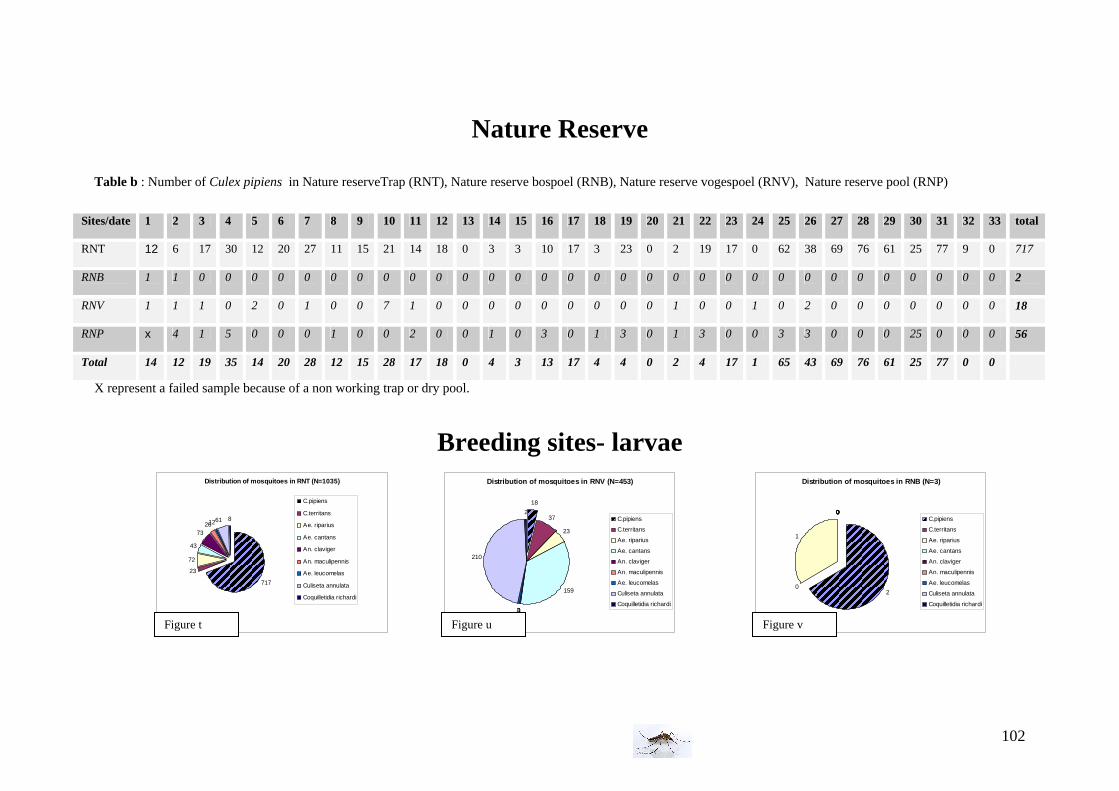
102

Nature Reserve

Table b : Number of Culex pipiens in Nature reserveTrap (RNT), Nature reserve bospoel (RNB), Nature reserve vogespoel (RNV), Nature reserve pool (RNP)

X represent a failed sample because of a non working trap or dry pool.

Breeding sites- larvae

Sites/date 1 2 3 4 5 6 7 8 9 10 11 12 13 14 15 16 17 18 19 20 21 22 23 24 25 26 27 28 29 30 31 32 33 total

RNT 12 6 17 30 12 20 27 11 15 21 14 18 0 3 3 10 17 3 23 0 2 19 17 0 62 38 69 76 61 25 77 9 0 717

RNB 1 1 0 0 0 0 0 0 0 0 0 0 0 0 0 0 0 0 0 0 0 0 0 0 0 0 0 0 0 0 0 0 0 2

RNV 1 1 1 0 2 0 1 0 0 7 1 0 0 0 0 0 0 0 0 0 1 0 0 1 0 2 0 0 0 0 0 0 0 18

RNP x 4 1 5 0 0 0 1 0 0 2 0 0 1 0 3 0 1 3 0 1 3 0 0 3 3 0 0 0 25 0 0 0 56

Total 14 12 19 35 14 20 28 12 15 28 17 18 0 4 3 13 17 4 4 0 2 4 17 1 65 43 69 76 61 25 77 0 0

Distribution of mosquitoes in RNT (N=1035)

861122673

43

72

23

717

C.pipiens

C.territans

Ae. riparius

Ae. cantans

An. claviger

An. maculipennis

Ae. leucomelas

Culiseta annulata


Distribution of mosquitoes in RNV (N=453)

2

210

301

159

23

37

18

C.pipiens

C.territans

Ae. riparius

Ae. cantans

An. claviger

An. maculipennis

Ae. leucomelas

Culiseta annulata


Distribution of mosquitoes in RNB (N=3)

000000

1

02

C.pipiens

C.territans

Ae. riparius

Ae. cantans

An. claviger

An. maculipennis

Ae. leucomelas

Culiseta annulata


Figure t Figure u Figure v

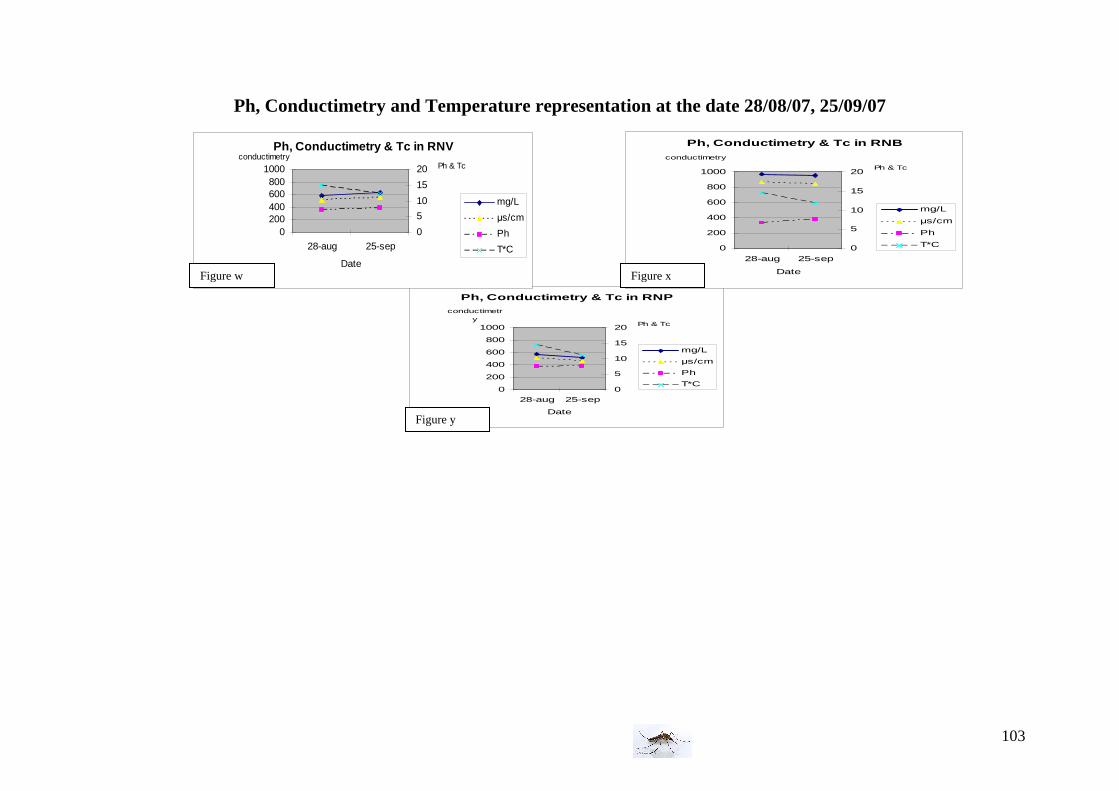
103

Ph, Conductimetry & Tc in RNP

0

200

400

600

800

1000

28-aug 25-sep

Date

conductimetry

0

5

10

15

20 Ph & Tc

mg/L

µs/cm

Ph

T*C

Ph, Conductimetry & Tc in RNV

0200400600800

1000

28-aug 25-sep

Date

conductimetry

0

5

10

15

20 Ph & Tc

mg/L

µs/cm

Ph

T*C

Ph, Conductimetry & Tc in RNB

0

200

400

600

800

1000

28-aug 25-sep

Date

conductimetry

0

5

10

15

20Ph & Tc

mg/L

µs/cm

Ph

T*C

Figure w Figure x

Figure y


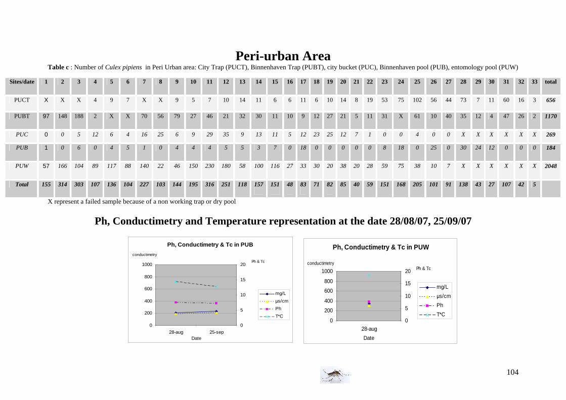
104

Ph, Conductimetry & Tc in PUB

0

200

400

600

800

1000

28-aug 25-sepDate

conductimetry

0

5

10

15

20Ph & Tc

mg/L

µs/cm

Ph

T*C

Ph, Conductimetry & Tc in PUW

0

200

400

600

800

1000

28-aug

Date

conductimetry

0

5

10

15

20 Ph & Tc

mg/L

µs/cm

Ph

T*C

Peri-urban Area Table c : Number of Culex pipiens in Peri Urban area: City Trap (PUCT), Binnenhaven Trap (PUBT), city bucket (PUC), Binnenhaven pool (PUB), entomology pool (PUW)

X represent a failed sample because of a non working trap or dry pool


Sites/date 1 2 3 4 5 6 7 8 9 10 11 12 13 14 15 16 17 18 19 20 21 22 23 24 25 26 27 28 29 30 31 32 33 total

PUCT X X X 4 9 7 X X 9 5 7 10 14 11 6 6 11 6 10 14 8 19 53 75 102 56 44 73 7 11 60 16 3 656

PUBT 97 148 188 2 X X 70 56 79 27 46 21 32 30 11 10 9 12 27 21 5 11 31 X 61 10 40 35 12 4 47 26 2 1170

PUC 0 0 5 12 6 4 16 25 6 9 29 35 9 13 11 5 12 23 25 12 7 1 0 0 4 0 0 X X X X X X 269

PUB 1 0 6 0 4 5 1 0 4 4 4 5 5 3 7 0 18 0 0 0 0 0 8 18 0 25 0 30 24 12 0 0 0 184

PUW 57 166 104 89 117 88 140 22 46 150 230 180 58 100 116 27 33 30 20 38 20 28 59 75 38 10 7 X X X X X X 2048

Total 155 314 303 107 136 104 227 103 144 195 316 251 118 157

151

48

83

71 82

85 40 59 151 168 205 101 91 138 43 27 107 42 5

Documents

Predictions West Nile Virus risk in the North