Prediction of solubility of ammonia in liquid …Prediction of solubility of ammonia in liquid electrolytes using Least Square Support Vector Machines Alireza Baghbana, Mohammad Bahadorib,

Ain Shams Engineering Journal (2016) xxx, xxx–xxx

Ain Shams University

Ain Shams Engineering Journal

www.elsevier.com/locate/asejwww.sciencedirect.com

ENGINEERING PHYSICS AND MATHEMATICS

Prediction of solubility of ammonia in liquid

electrolytes using Least Square Support Vector

Machines

* Corresponding author at: School of Environment, Science and

Engineering, Southern Cross University, Lismore, NSW, Australia.

E-mail address: [email protected] (A. Bahadori).

Peer review under responsibility of Ain Shams University.

Production and hosting by Elsevier

http://dx.doi.org/10.1016/j.asej.2016.08.0062090-4479 � 2016 Ain Shams University. Production and hosting by Elsevier B.V.This is an open access article under the CC BY-NC-ND license (http://creativecommons.org/licenses/by-nc-nd/4.0/).

Please cite this article in press as: Baghban A et al., Prediction of solubility of ammonia in liquid electrolytes using Least Square Support Vector Machines, AiEng J (2016), http://dx.doi.org/10.1016/j.asej.2016.08.006

Alireza Baghbana, Mohammad Bahadori

b, Alireza Samadi Lemraski

c,

Alireza Bahadori d,e,*

aYoung Researcher and Elite Club, Marvdasht Branch, Islamic Azad University, Marvdasht, IranbSchool of Environment, Griffith University, Nathan, QLD, AustraliacDepartment of Gas Engineering, Ahwaz Faculty of Petroleum Engineering, Petroleum University of Technology (PUT),

P.O. Box 63431, Ahwaz, IrandSchool of Environment, Science and Engineering, Southern Cross University, Lismore, NSW, AustraliaeAustralian Oil and Gas Services, Pty Ltd, Lismore, NSW 2480, Australia

Received 28 July 2015; revised 14 July 2016; accepted 17 August 2016

KEYWORDS

Ammonia;

Solubility;

Ionic liquid;

Support Vector Machine

Abstract Liquid electrolytes or ionic liquids (ILs) are a new class of environmentally friendly sol-

vents which is highly promising for refrigeration and air conditioning applications in chemical

industrial processes.

In this contribution, Least Square Support Vector Machine (LS-SVM) models have been utilized

to predict the solubility of ammonia in ILs as a function of molecular weight (MW), critical tem-

perature (Tc) and critical pressure (Pc) of pure ILs over wide ranges of temperature, pressure, and

concentration. To this end, 352 experimental data points were collected from the published papers.

Moreover, to verify the accuracy of the proposed models, statistical analyses such as regression

coefficient, mean square error (MSE), average absolute deviation (AAD), standard deviation

(STD) and root mean square error (RMSE) have been conducted on the calculated values. The

results show the excellent performance of LSSVM models to predict the solubility of ammonia in

different liquid electrolytes.� 2016 Ain Shams University. Production and hosting by Elsevier B.V. This is an open access article under

the CC BY-NC-ND license (http://creativecommons.org/licenses/by-nc-nd/4.0/).

1. Introduction

Total world energy consumption is different from actual world

energy usage due to energy loss. Therefore, seeking practicalways to use low-grade heat, such as waste heat, solar energy,and biomass aroused considerable interest [1–4]. One efficient

method of using low-grade heat is the absorption refrigeration

n Shams

http://creativecommons.org/licenses/by-nc-nd/4.0/

mailto:[email protected]

http://dx.doi.org/10.1016/j.asej.2016.08.006


http://www.sciencedirect.com/science/journal/20904479


http://creativecommons.org/licenses/by-nc-nd/4.0/


2 A. Baghban et al.

cycles instead of the commonly-employed vapor-compressioncycles which consume a high amount of energy to elevate therefrigerant pressure [1,3] and also contribute to the ozone layer

depletion and the greenhouse effect [5]. The economical usageof waste heat is the main advantage of absorption refrigerationcycles since it reduces the detrimental effect of lost heat on the

environment [6,7].The commonly used working pairs in absorption cycles are

aqueous solutions of either lithium bromide (H2O/LiBr) or

ammonia (NH3/H2O) have serious disadvantages in industrialapplications such as corrosion, crystallization, high workingpressure, and toxicity [7,8]. Besides, the strong affinity betweenNH3 and H2O causes high running costs due to the large heat

consumption to separate NH3 from H2O [9]. Thus, it may benecessary to develop alternative solvents that absorb highamounts of NH3 along with low separation process cost.

Recently, ionic liquids (ILs) as novel solvent species are intro-duced for absorption refrigeration cycles [8,10–13].

An ionic liquid is defined as a salt with unwell coordinated

ions which leads to the fact that these solvents turn into liquidin temperatures less than 100 �C or even at some points such asroom temperature (room temperature ionic liquids, RTILs).

At least one ion has a delocalized charge and one componentis organic, which prevents the formation of a stable crystallattice.

The main advantage of an ionic liquid is that it practically

exerts no vapor pressure [14–16] while offering the benefits ofconventional solvents that have high volatility. Their proper-ties, such as viscosity, melting point, density, and hydropho-

bicity, may be adjusted to meet the desired conditions by acombination of cations and anions [17].

Besides, high heat capacity, non-flammability, low-

corrosive character, non-toxicity and large capacity for dis-solving, for example, H2O and NH3 [10], are their other advan-tages that make them interesting for industrial applications as

solvents in organic synthesis, homogeneous and biphasic trans-fer catalysts, for electrical deposition and applications inmembrane-based systems for separation [17].

For an efficient and economical design of chemical pro-

cesses and separation operations, it is vital to have precisevapor-liquid equilibrium data [17,18]. Mainly, equations ofstate have been used to study the phase behavior of the system

containing different gasses + ionic liquids in the open litera-ture [19–23].

Despite the fact that, equations of state are playing an

expanding role in the accurate calculation of fluid phase equi-libria and can be used over wide ranges of temperature andpressure including subcritical and supercritical regions but,for the systems containing complicated molecules, more

sophisticated approach is required for understanding the inter-actions between unlike molecules.

Also, an appropriate mixing rule is crucial to achieving con-

siderable progress in phase behavior calculations using equa-tions of state [24]. Thus, for the best representation of non-ideal systems, binary interaction parameters from a regression

of experimental VLE data should be obtained. The iterativemethod for the estimation of VLE using EOS makes it unsuit-able for real-time control [24,25].

Also, taking into account the difficulties of conductingexperiments and also their high operational costs in somecases, application of new estimation methods such as artificialintelligence machine techniques has proved to be exceptionally

Please cite this article in press as: Baghban A et al., Prediction of solubility of ammonEng J (2016), http://dx.doi.org/10.1016/j.asej.2016.08.006

useful and of interest in chemical engineering [17,26]. Recently,these new techniques have been applied to estimate thermody-namic properties, VLE data, liquid phase activity coefficient,

shape and compressibility factors for several refrigerants andattracted considerable interest because of their successful out-puts [27,28]. Fuzzy Logic System (FLS), Artificial Neural Net-

work (ANN), Adaptive Neuro-Fuzzy Inference System(ANFIS) and Support Vector Machine (SVM) are the com-monly used embranchment of computational intelligence

paradigms.SVMs are the newer ones and in the past decades, better

performance with a more accurate approximation of SVMshad been shown against other previous intelligent approaches

[29,30]. Like the other abovementioned approaches, they canapply for classification and regression problems.

In the current study, SVM and LS-SVM models are devel-

oped for estimating ammonia solubility in [bmim][PF6],[bmim][BF4], [emim][Tf2N], [hmim][Cl], [C2MIM][BF4],[C6MIM][BF4], [C8MIM][BF4], [emim][Ac], [emim][EtOSO3],

[emim][SCN], [DMEA][Ac], over wide ranges of temperature,concentration and pressure [31–33]. Furthermore, to compareresults of proposed models and experimental values, statistical

criteria are performed.

2. Theory

2.1. Support Vector Machine

According to the theory of statistical learning, support vectormachine (SVM) is a ubiquitous learning approach and it wasfirst proposed by Vapnik [34]. Furthermore, it has been mostlyused to solve regression problems and the obtained result is

often more accurate and better than other machine learningapproaches such as multi-layer perceptron artificial neural net-work and fuzzy logic system [35].

Based on the principle of structural risk minimization,SVM takes the fitting of training data and the complexity ofthe training sample into consideration [36]. Moreover, it can

predict the regression using a set of kernel functions whichare specified in a high dimensional feature space. Since theoptimality problem is convex, a unique solution is delivered.This is an advantage of SVM over Neural Networks, which

have multiple solutions associated with local minima [37].To describe regression with SVMs, Support vector regres-

sion (SVR) is used in the literature. Based on an assumed data

set (xi, yi)n, the regression assessment with SVR is used for esti-mating a function, where xi represents the input vector and yirepresents the target value and the total number of data sets

has been represented by n (herein, the input vectors (xi) referto temperature, pressure, critical temperature, critical pressureand molecular weight, whereas the target value (yi) refers to

mole fraction of ammonia). As formulated in Eq. (1), the lin-ear regression function uses the following function:

fðxÞ ¼ x � /ðxÞ þ b ð1Þ

where /(x) is a nonlinear function such as the polynomial,radial basis and Sigmoid functions, and the weight and bias

vectors have been represented by x and b respectively thatare calculated from the training data set. As formulated inEqs. (2) and (3), linear regression is accomplished in a highdimensional feature space using a nonlinear mapping and the

ia in liquid electrolytes using Least Square Support Vector Machines, Ain Shams


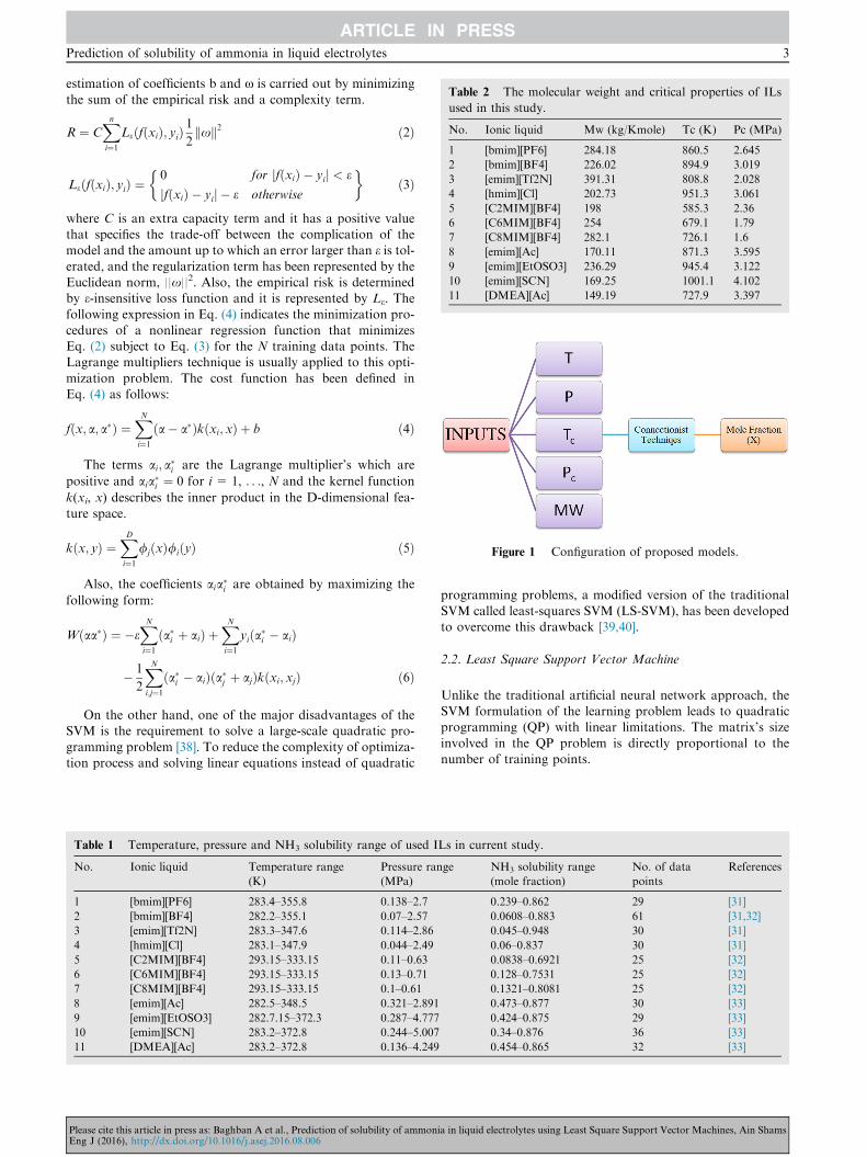
Table 2 The molecular weight and critical properties of ILs

used in this study.

No. Ionic liquid Mw (kg/Kmole) Tc (K) Pc (MPa)

1 [bmim][PF6] 284.18 860.5 2.645

2 [bmim][BF4] 226.02 894.9 3.019

3 [emim][Tf2N] 391.31 808.8 2.028

4 [hmim][Cl] 202.73 951.3 3.061

5 [C2MIM][BF4] 198 585.3 2.36

6 [C6MIM][BF4] 254 679.1 1.79

7 [C8MIM][BF4] 282.1 726.1 1.6

8 [emim][Ac] 170.11 871.3 3.595

9 [emim][EtOSO3] 236.29 945.4 3.122

10 [emim][SCN] 169.25 1001.1 4.102

11 [DMEA][Ac] 149.19 727.9 3.397

Figure 1 Configuration of proposed models.

Prediction of solubility of ammonia in liquid electrolytes 3

estimation of coefficients b and x is carried out by minimizing

the sum of the empirical risk and a complexity term.

R ¼ CXni¼1

LeðfðxiÞ; yiÞ1

2kxk2 ð2Þ

LeðfðxiÞ; yiÞ ¼0 for jfðxiÞ � yij < e

jfðxiÞ � yij � e otherwise

� �ð3Þ

where C is an extra capacity term and it has a positive valuethat specifies the trade-off between the complication of themodel and the amount up to which an error larger than e is tol-erated, and the regularization term has been represented by theEuclidean norm, ||x||2. Also, the empirical risk is determinedby e-insensitive loss function and it is represented by Le. The

following expression in Eq. (4) indicates the minimization pro-cedures of a nonlinear regression function that minimizesEq. (2) subject to Eq. (3) for the N training data points. TheLagrange multipliers technique is usually applied to this opti-

mization problem. The cost function has been defined inEq. (4) as follows:

fðx; a; a�Þ ¼XNi¼1

ða� a�Þkðxi; xÞ þ b ð4Þ

The terms ai; a�i are the Lagrange multiplier’s which are

positive and aia�i ¼ 0 for i= 1, . . ., N and the kernel function

k(xi, x) describes the inner product in the D-dimensional fea-ture space.

kðx; yÞ ¼XDi¼1

/jðxÞ/iðyÞ ð5Þ

Also, the coefficients aia�i are obtained by maximizing the

following form:

Wðaa�Þ ¼ �eXNi¼1

ða�i þ aiÞ þXNi¼1

yiða�i � aiÞ

� 1

2

XNi;j¼1

ða�i � aiÞða�j þ ajÞkðxi; xjÞ ð6Þ

On the other hand, one of the major disadvantages of theSVM is the requirement to solve a large-scale quadratic pro-

gramming problem [38]. To reduce the complexity of optimiza-tion process and solving linear equations instead of quadratic

Table 1 Temperature, pressure and NH3 solubility range of used I

No. Ionic liquid Temperature range

(K)

Pressure ran

(MPa)

1 [bmim][PF6] 283.4–355.8 0.138–2.7

2 [bmim][BF4] 282.2–355.1 0.07–2.57

3 [emim][Tf2N] 283.3–347.6 0.114–2.86

4 [hmim][Cl] 283.1–347.9 0.044–2.49

5 [C2MIM][BF4] 293.15–333.15 0.11–0.63

6 [C6MIM][BF4] 293.15–333.15 0.13–0.71

7 [C8MIM][BF4] 293.15–333.15 0.1–0.61

8 [emim][Ac] 282.5–348.5 0.321–2.891

9 [emim][EtOSO3] 282.7.15–372.3 0.287–4.777

10 [emim][SCN] 283.2–372.8 0.244–5.007

11 [DMEA][Ac] 283.2–372.8 0.136–4.249


programming problems, a modified version of the traditional

SVM called least-squares SVM (LS-SVM), has been developedto overcome this drawback [39,40].

2.2. Least Square Support Vector Machine

Unlike the traditional artificial neural network approach, theSVM formulation of the learning problem leads to quadraticprogramming (QP) with linear limitations. The matrix’s size

involved in the QP problem is directly proportional to thenumber of training points.

Ls in current study.

ge NH3 solubility range

(mole fraction)

No. of data

points

References

0.239–0.862 29 [31]

0.0608–0.883 61 [31,32]

0.045–0.948 30 [31]

0.06–0.837 30 [31]

0.0838–0.6921 25 [32]

0.128–0.7531 25 [32]

0.1321–0.8081 25 [32]

0.473–0.877 30 [33]

0.424–0.875 29 [33]

0.34–0.876 36 [33]

0.454–0.865 32 [33]



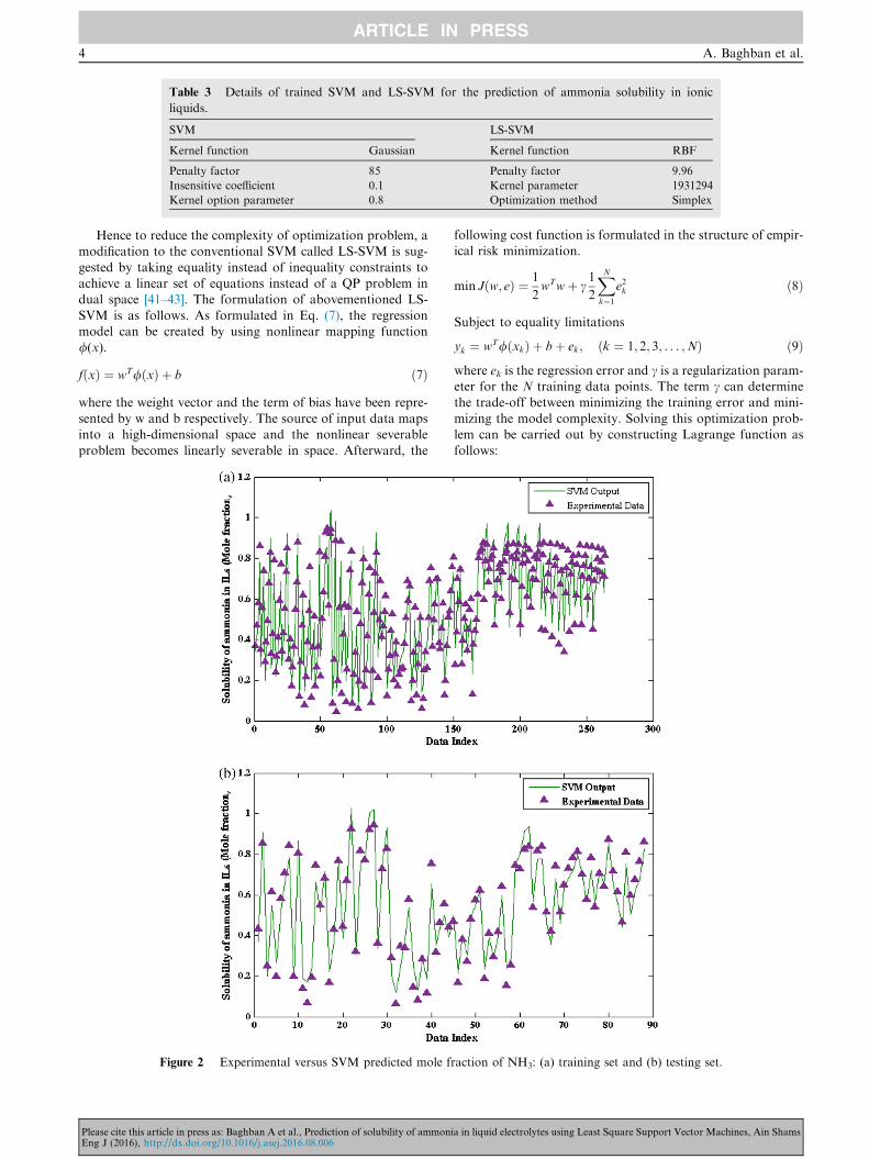
Table 3 Details of trained SVM and LS-SVM for the prediction of ammonia solubility in ionic

liquids.

SVM LS-SVM

Kernel function Gaussian Kernel function RBF

Penalty factor 85 Penalty factor 9.96

Insensitive coefficient 0.1 Kernel parameter 1931294

Kernel option parameter 0.8 Optimization method Simplex

4 A. Baghban et al.

Hence to reduce the complexity of optimization problem, amodification to the conventional SVM called LS-SVM is sug-

gested by taking equality instead of inequality constraints toachieve a linear set of equations instead of a QP problem indual space [41–43]. The formulation of abovementioned LS-

SVM is as follows. As formulated in Eq. (7), the regressionmodel can be created by using nonlinear mapping function/(x).

fðxÞ ¼ wT/ðxÞ þ b ð7Þwhere the weight vector and the term of bias have been repre-

sented by w and b respectively. The source of input data mapsinto a high-dimensional space and the nonlinear severableproblem becomes linearly severable in space. Afterward, the

Figure 2 Experimental versus SVM predicted mole f


following cost function is formulated in the structure of empir-ical risk minimization.

min Jðw; eÞ ¼ 1

2wTwþ c

1

2

XNk¼1

e2k ð8Þ

Subject to equality limitations

yk ¼ wT/ðxkÞ þ bþ ek; ðk ¼ 1; 2; 3; . . . ;NÞ ð9Þwhere ek is the regression error and c is a regularization param-eter for the N training data points. The term c can determinethe trade-off between minimizing the training error and mini-

mizing the model complexity. Solving this optimization prob-lem can be carried out by constructing Lagrange function asfollows:

raction of NH3: (a) training set and (b) testing set.



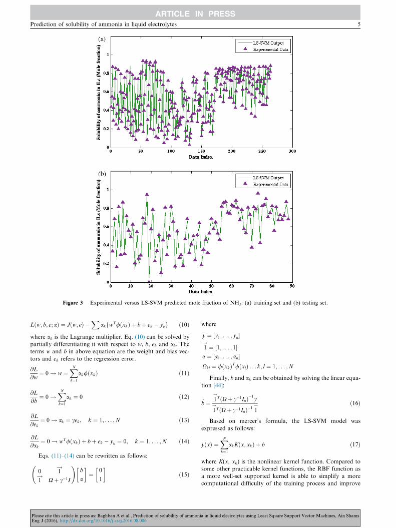
Figure 3 Experimental versus LS-SVM predicted mole fraction of NH3: (a) training set and (b) testing set.


Lðw; b; e; aÞ ¼ Jðw; eÞ �X

akfwT/ðxkÞ þ bþ ek � ykg ð10Þwhere ak is the Lagrange multiplier. Eq. (10) can be solved bypartially differentiating it with respect to w, b, ek and ak. Theterms w and b in above equation are the weight and bias vec-

tors and ek refers to the regression error.

@L

@w¼ 0 ! w ¼

XNk¼1

ak/ðxkÞ ð11Þ

@L

@b¼ 0 !

XNk¼1

ak ¼ 0 ð12Þ

@L

@ek¼ 0 ! ak ¼ cek; k ¼ 1; . . . ;N ð13Þ

@L

@ak¼ 0 ! wT/ðxkÞ þ bþ ek � yk ¼ 0; k ¼ 1; . . . ;N ð14Þ

Eqs. (11)–(14) can be rewritten as follows:

0 1!

1!

Xþ c�1I

!b

a

� �¼ 0

1

� �ð15Þ


where

y ¼ ½y1; . . . ; yn�1!¼ ½1; . . . ; 1�

a ¼ ½a1; . . . ; an�Xkl ¼ /ðxkÞT/ðxlÞ . . . k; l ¼ 1; . . . ;N

Finally, b and ak can be obtained by solving the linear equa-

tion [44]:

b ¼ 1!TðXþ c�1InÞ�1

y

1!TðXþ c�1InÞ�1

1! ð16Þ

Based on mercer’s formula, the LS-SVM model was

expressed as follows:

yðxÞ ¼XNk¼1

akKðx; xkÞ þ b ð17Þ

where K(x, xk) is the nonlinear kernel function. Compared tosome other practicable kernel functions, the RBF function asa more well-set supported kernel is able to simplify a morecomputational difficulty of the training process and improve



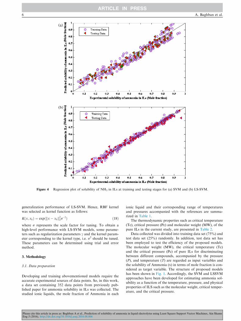
Figure 4 Regression plot of solubility of NH3 in ILs at training and testing stages for (a) SVM and (b) LS-SVM.

6 A. Baghban et al.

generalization performance of LS-SVM. Hence, RBF kernelwas selected as kernel function as follows:

Kðx; xkÞ ¼ expðkx� xkk22r�2Þ ð18Þwhere r represents the scale factor for tuning. To obtain ahigh-level performance with LS-SVM models, some parame-ters such as regularization parameters c and the kernel param-

eter corresponding to the kernel type, i.e. r2 should be tuned.These parameters can be determined using trial and errormethod.

3. Methodology

3.1. Data preparation

Developing and training abovementioned models require the

accurate experimental sources of data points. So, in this work,a data set containing 352 data points from previously pub-lished paper for ammonia solubility in ILs was collected. Thestudied ionic liquids, the mole fraction of Ammonia in each


ionic liquid and their corresponding range of temperatures

and pressures accompanied with the references are summa-rized in Table 1.

The thermodynamic properties such as critical temperature

(Tc), critical pressure (Pc) and molecular weight (MW), of thepure ILs in the current study, are presented in Table 2.

Data collected was divided into training data set (75%) and

test data set (25%) randomly. In addition, test data set hasbeen employed to test the efficiency of the proposed models.The molecular weight (MW), the critical temperature (Tc)

and the critical pressure (Pc) of pure ILs for discriminatingbetween different compounds, accompanied by the pressure(P), and temperature (T) are regarded as input variables andthe solubility of Ammonia (x) in terms of mole fraction is con-

sidered as target variable. The structure of proposed modelshas been shown in Fig. 1. Accordingly, the SVM and LSSVMapproaches have been developed for estimating ammonia sol-

ubility as a function of the temperature, pressure, and physicalproperties of ILS such as the molecular weight, critical temper-ature, and the critical pressure.



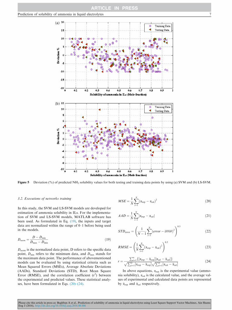
Figure 5 Deviation (%) of predicted NH3 solubility values for both testing and training data points by using (a) SVM and (b) LS-SVM.


3.2. Executions of networks training

In this study, the SVM and LS-SVM models are developed for

estimation of ammonia solubility in ILs. For the implementa-tion of SVM and LS-SVM models, MATLAB software has

been used. As formulated in Eq. (19), the inputs and targetdata are normalized within the range of 0–1 before being usedin the models.

Dnorm ¼ D�Dmin

Dmax �Dmin

ð19Þ

Dnorm is the normalized data point, D refers to the specific datapoint, Dmin refers to the minimum data, and Dmax stands for

the maximum data point. The performance of abovementionedmodels can be evaluated by using statistical criteria such asMean Squared Errors (MSEs), Average Absolute Deviations

(AADs), Standard Deviations (STD), Root Mean SquareError (RMSE), and the correlation coefficient (r2) betweenthe experimental and predicted values. These statistical analy-ses, have been formulated in Eqs. (20)–(24).


MSE ¼ 1

N

XNi¼1

ðaexp � acalÞ2 ð20Þ

AAD ¼ 1

N

XNi¼1

jaexp � acalj ð21Þ

STDerror ¼ 1

N� 1

XNi¼1

ðerror� errorÞ2 !0:5

ð22Þ

RMSE ¼ 1

N

XNi¼1

ðaexp � acalÞ2 !0:5

ð23Þ

r ¼Pn

i¼1f½aexp � �aexp�½acal � �acal�gffiffiffiffiffiffiffiffiffiffiffiffiffiffiffiffiffiffiffiffiffiffiffiffiffiffiffiffiffiffiffiffiffiffiPni¼1½aexp � �aexp�

p ffiffiffiffiffiffiffiffiffiffiffiffiffiffiffiffiffiffiffiffiffiffiffiffiffiffiffiffiffiffiffiffiPni¼1½acal � �acal�

p ð24Þ

In above equations, aexp is the experimental value (ammo-

nia solubility), acal is the calculated value, and the average val-

ues of experimental and calculated data points are representedby �aexp and �acal respectively.



Table 4 Comparison between the performances of SVM and

LS-SVM models.

Network SVM LS-SVM

Analysis Training Testing Training Testing

R2 0.968 0.9734 0.9961 0.9915

MSE 0.0038 0.0031 4.596e�4 9.433e�4

AAD 0.0521 0.0484 0.0158 0.0223

RMSE 0.0614 0.0559 0.0214 0.0307

Standard deviation 0.0326 0.0281 0.0145 0.0213

8 A. Baghban et al.

4. Results and discussion

In the current study, SVM and LS-SVM models have beenemployed to approximate the nonlinear relationship between

input and target variables. Among 352 experimental datapoints reported in the literature for ammonia solubility inILs, 264 data points as the training set and 88 points of data

bank as the testing set, which were not used during the trainingprocess, were employed to implement the SVM and LS-SVMmodels. It is important to note that all of the ILs existing inthe training data set are employed in the test data set.

There are three parameters that require being set in SVMmodel before training, namely, penalty factor C, insensitivecoefficient e and kernel function K. Selecting the type of kernel

and its parameters is typically based on application domainknowledge which reflects the distribution of input values ofthe training data sets [35,36]. Based on the analysis of training

data sets, we choose Gaussian Function as K and kernel optionparameter P is set to 0.8. We set C to 85 and e to 0.1. For LS-SVM model, there are only two parameters need to be deter-

mined, namely, regularization parameters c and the kernelparameter r2. Tuning of these parameters was conducted intwo steps.

First, a state-of-the-art global optimization technique, Cou-

pled Simulated Annealing (CSA), determined suitable param-eters based on some criterion. Second, these parameters werethen given to a second optimization procedure, simplex or grid

search, to perform a fine-tuning step. According to these pro-cedures, r2 in RBF regularization parameters and c obtained9.96 and 1,931,294 respectively. Details of SVM and LS-

SVM models have been summarized in Table 3.To demonstrate a superior visual comparison, the target,

and estimated values are plotted as a function of the number

of data points simultaneously in Figs. 2 and 3 for both modelsin current work at training and testing stages. The lines in thesefigures are regressed from the SVM and LS-SVM modelsrespectively and triangles are the experimental values of

ammonia solubility for both training and testing stages.According to obtained results, the predicted values by LS-SVM model have excellent agreement with experimental val-

ues, while obtained results from the SVMmodel are not as wellaccurate as LS-SVM. The regression plots of proposed modelshave been shown in Fig. 4 between model results and experi-

mental corresponding values. A close-fitting of data pointsabout the 45� line for both models indicates their reliability.

Based on these Figures, the outputs of LS-SVM are verywell in agreement with experimental corresponding values

and the regression coefficient of it is 0.9961 for training and0.9915 for the testing data set. Also, the regression coefficient


of SVM obtained 0.968 for training and 0.9734 for the testingdata set.

According to the statistical viewpoints, Eqs. (25) and (26)

were generated as linear regressions for LS-SVM and SVMmodels respectively for the test data set correspondingly

y ¼ 0:96xþ 0:025; R2 ¼ 0:99145 ð25Þ

y ¼ 0:95xþ 0:02; R2 ¼ 0:97342 ð26ÞThe percent of relative deviation between experimental data

and proposed output of models is shown in Fig. 5.While the AADs% of testing and training data points for

LS-SVM are 2.2252% and 1.5797% respectively, the AAD%

of SVM outputs from corresponding experimental data pointsobtained 5.2104% and 4.8432% at training and testing stagesrespectively.

To verify the proposed models, statistical analyses such asregression coefficient (r2), Mean Square Error (MSE), AverageAbsolute Deviation (AAD), Standard Deviation (STD) and

Root Mean Square Error (RMSE) have been conducted onobtained results. Results of statistical analyses have been sum-marized in Table 4 for both models at testing and trainingstages.

5. Conclusion

In this study, based on experimental data gathered from thepreviously published papers, a Support Vector Machine(SVM) and a Least Square Support Vector Machine (LS-SVM) were developed for estimating of ammonia solubility

in various ionic liquids (ILs) over wide ranges of temperature,pressure, and concentration.

To propose a reliable model, 13 various ILs were employed.

The molecular weight (Mw), the critical pressure (Pc) and thecritical temperature (Tc) of ILs accompanied by the pressure(P) and temperature (T) were used as input variables and mole

fraction of ammonia was used as target variable of frame-works. Results from the statistical analyses confirmed accept-able predictive capability of both models, but the LS-SVMoutput was more accurate than the SVM model in order to

estimate ammonia solubility in the ILs. One of the major dis-advantages of the SVM against the LS-SVM was its require-ment to solve a large-scale quadratic programming problem,

while the LS-SVM reduces the complexity of optimization pro-cess and solving linear equations instead of quadratic pro-gramming problems. These developed tools, especially the

LS-SVM model can be of immense help for chemists andchemical engineers to have simple predictive tools against dif-ficult thermodynamic approaches for estimating ammonia sol-

ubility as a function of the temperature, pressure, and physicalproperties of ILs such as the molecular weight, the criticalpressure, and the critical temperature.

References

[1] Sun G, Huang W, Zheng D, Dong L, Wu X. Vapor-liquid

equilibrium prediction of ammonia-ionic liquid working pairs of

absorption cycle using UNIFAC model. Chin J Chem Eng

2014;22:72–8.

[2] Wu T, Wu Y, Yu Z, Zhao H, Wu H. Experimental investigation

on an ammonia–water–lithium bromide absorption refrigeration


http://refhub.elsevier.com/S2090-4479(16)30116-2/h0005








system without solution pump. Energy Convers Manage

2011;52:2314–9.

[3] Aphornratana S, Sriveerakul T. Analysis of a combined Rankine–

vapour–compression refrigeration cycle. Energy Convers Manage

2010;51:2557–64.

[4] Cai D, He G, Tian Q, Tang W. Thermodynamic analysis of a

novel air-cooled non-adiabatic absorption refrigeration cycle

driven by low grade energy. Energy Convers Manage

2014;86:537–47.

[5] Gomri R. Second law comparison of single effect and double

effect vapour absorption refrigeration systems. Energy Convers

Manage 2009;50:1279–87.

[6] Srikhirin P, Aphornratana S, Chungpaibulpatana S. A review of

absorption refrigeration technologies. Renew Sustain Energy Rev

2001;5:343–72.

[7] Gogoi TK, Talukdar K. Thermodynamic analysis of a combined

reheat regenerative thermal power plant and water–LiBr vapor

absorption refrigeration system. Energy Convers Manage

2014;78:595–610.

[8] Sun J, Fu L, Zhang S. A review of working fluids of absorption

cycles. Renew Sustain Energy Rev 2012;16:1899–906.

[9] McLinden MO, Radermacher R. Experimental comparison of

ammonia-water and ammonia-water lithium bromide mixtures in

an absorption heat pump ASHRAE technical data bulletin (p. 52–

60) AND. ASHRAE Trans 1985;91:1837–46.

[10] Khamooshi M, Parham K, Atikol U. Overview of ionic liquids

used as working fluids in absorption cycles. Adv Mech Eng

2013;2013:7.

[11] Kim YJ, Kim S, Joshi YK, Fedorov AG, Kohl PA. Thermody-

namic analysis of an absorption refrigeration system with ionic-

liquid/refrigerant mixture as a working fluid. Energy

2012;44:1005–16.

[12] Kim S, Kohl PA. Theoretical and experimental investigation of an

absorption refrigeration system using R134/[bmim][PF6] working

fluid. Ind Eng Chem Res 2013;52:13459–65.

[13] Kim S, Patel N, Kohl PA. Performance simulation of ionic liquid

and hydrofluorocarbon working fluids for an absorption refrig-

eration system. Ind Eng Chem Res 2013;52:6329–35.

[14] Ayou DS, Curras MR, Salavera D, Garcıa J, Bruno JC, Coronas

A. Performance analysis of absorption heat transformer cycles

using ionic liquids based on imidazolium cation as absorbents

with 2,2,2-trifluoroethanol as refrigerant. Energy Convers Man-

age 2014;84:512–23.

[15] Wang G, Zhang S, Xu W, Qi W, Yan Y, Xu Q. Efficient

saccharification by pretreatment of bagasse pith with ionic liquid

and acid solutions simultaneously. Energy Convers Manage

2015;89:120–6.

[16] Auxenfans T, Buchoux S, Larcher D, Husson G, Husson E,

Sarazin C. Enzymatic saccharification and structural properties of

industrial wood sawdust: recycled ionic liquids pretreatments.

Energy Convers Manage 2014;88:1094–103.

[17] Eslamimanesh A, Gharagheizi F, Mohammadi AH, Richon D.

Artificial neural network modeling of solubility of supercritical

carbon dioxide in 24 commonly used ionic liquids. Chem Eng Sci

2011;66:3039–44.

[18] Coquelet C, Rivollet F, Jarne C, Valtz A, Richon D. Measure-

ment of physical properties of refrigerant mixtures. Determination

of phase diagrams. Energy Convers Manage 2006;47:3672–80.

[19] Shariati A, Peters CJ. High-pressure phase behavior of systems

with ionic liquids: Part III. The binary system carbon dioxide +

1-hexyl-3-methylimidazolium hexafluorophosphate. J Supercrit

Fluids 2004;30:139–44.

[20] Valderrama JO, Reategui A, Sanga WW. Thermodynamic con-

sistency test of vapor�liquid equilibrium data for mixtures

containing ionic liquids. Ind Eng Chem Res 2008;47:8416–22.

[21] Alvarez VH, Larico R, Ianos Y, Aznar M. Parameter estimation

for VLE calculation by global minimization: the genetic algo-

rithm. Braz J Chem Eng 2008;25:409–18.


[22] Vega LF, Vilaseca O, Llovell F, Andreu JS. Modeling ionic

liquids and the solubility of gases in them: recent advances and

perspectives. Fluid Phase Equilib 2010;294:15–30.

[23] Valderrama JO, Urbina F, Faundez CA. Gas–liquid equilibrium

modeling of mixtures containing supercritical carbon dioxide and

an ionic liquid. J Supercrit Fluids 2012;64:32–8.

[24] Karimi H, Yousefi F. Correlation of vapour liquid equilibria of

binary mixtures using artificial neural networks. Chin J Chem Eng

2007;15:765–71.

[25] Faundez CA, Quiero FA, Valderrama JO. Phase equilibrium

modeling in ethanol + congener mixtures using an artificial

neural network. Fluid Phase Equilib 2010;292:29–35.

[26] Lashkarbolooki M, Vaferi B, Shariati A, Zeinolabedini A.

Hezave, Investigating vapor–liquid equilibria of binary mixtures

containing supercritical or near-critical carbon dioxide and a

cyclic compound using cascade neural network. Fluid Phase

Equilib 2013;343:24–9.

[27] Ketabchi S, Ghanadzadeh H, Ghanadzadeh A, Fallahi S, Ganji

M. Estimation of VLE of binary systems (tert-butanol + 2-ethyl-

1-hexanol) and (n-butanol + 2-ethyl-1-hexanol) using GMDH-

type neural network. J Chem Thermodyn 2010;42:1352–5.

[28] Gilani HG, Samper KG, Haghi RK. Chemoinformatics:

advanced control and computational techniques. CRC Press;

2012.

[29] Chorowski J, Wang J, Zurada JM. Review and performance

comparison of SVM- and ELM-based classifiers. Neurocomput-

ing 2014;128:507–16.

[30] Ahmad AS, Hassan MY, Abdullah MP, Rahman HA, Hussin F,

Abdullah H, Saidur R. A review on applications of ANN and

SVM for building electrical energy consumption forecasting.

Renew Sustain Energy Rev 2014;33:102–9.

[31] Yokozeki A, Shiflett MB. Ammonia solubilities in room-temper-

ature ionic liquids. Ind Eng Chem Res 2007;46:1605–10.

[32] Yokozeki A, Shiflett MB. Vapor–liquid equilibria of ammonia

+ ionic liquid mixtures. Appl Energy 2007;84:1258–73.

[33] Chen W, Liang S, Guo Y, Gui X, Tang D. Investigation on

vapor–liquid equilibria for binary systems of metal ion-containing

ionic liquid [bmim]Zn2Cl5/NH3 by experiment and modified

UNIFAC model. Fluid Phase Equilib 2013;360:1–6.

[34] Vapnik V. Statistical learning theory. New York: Wiley; 1998.

[35] Li Q, Meng Q, Cai J, Yoshino H, Mochida A. Predicting hourly

cooling load in the building: a comparison of support vector

machine and different artificial neural networks. Energy Convers

Manage 2009;50:90–6.

[36] Fei S-W, Wang M-J, Miao Y-B, Tu J, Liu C-L. Particle swarm

optimization-based support vector machine for forecasting dis-

solved gases content in power transformer oil. Energy Convers

Manage 2009;50:1604–9.

[37] Anguita D, Ghio A, Greco N, Oneto L, Ridella S. Model selection

for support vector machines: advantages and disadvantages of the

machine learning theory. In: The 2010 international joint confer-

ence on neural networks (IJCNN). p. 1–8.

[38] Sattari M, Gharagheizi F, Ilani-Kashkouli P, Mohammadi AH,

Ramjugernath D. Determination of the speed of sound in ionic

liquids using a least squares support vector machine group

contribution method. Fluid Phase Equilib 2014;367:188–93.

[39] Ekici BB. A least squares support vector machine model for

prediction of the next day solar insolation for effective use of PV

systems. Measurement 2014;50:255–62.

[40] Haijun T, Jingru W. Modeling of power plant superheated steam

temperature based on least squares support vector machines.

Energy Procedia 2012;17(Part A):61–7.

[41] Esteki M, Rezayat M, Ghaziaskar HS, Khayamian T. Application

of QSPR for prediction of percent conversion of esterification

reactions in supercritical carbon dioxide using least squares

support vector regression. J Supercrit Fluids 2010;54:222–30.

[42] Mesbah M, Soroush E, Azari V, Lee M, Bahadori A, Habibnia S.

Vapor liquid equilibrium prediction of carbon dioxide and























































































































































10 A. Baghban et al.

hydrocarbon systems using LSSVM algorithm. J Supercrit Fluids

2015;97:256–67.

[43] Gharagheizi F, Ilani-Kashkouli P, Sattari M, Mohammadi AH,

Ramjugernath D, Richon D. Development of a LSSVM-GC

model for estimating the electrical conductivity of ionic liquids.

Chem Eng Res Des 2014;92:66–79.

[44] Suykens JAK, De Brabanter J, Lukas L, Vandewalle J. Weighted

least squares support vector machines: robustness and sparse

approximation. Neurocomputing 2002;48:85–105.

Alireza Baghban is a PhD research student in

the Amirkabir University of Technology,

Mahshahr Campus, Mahshahr, Iran. He

received his B.Sc. degree from the University

of Tehran and a M.Sc. degree from the Pet-

roleum University of Technology (Ahwaz,

Iran).

Mohammad Bahadori is a PhD research stu-

dent in the School of Environment, Griffith

University, Nathan Campus, QLD, Australia.

He received his B.Sc. degree from Shahaid

Chamran University (Ahwaz, Iran) and a

M.Sc. degree from the University of Tehran.

Alireza Samadi Lemraski is a graduate Msc

student with Department of Gas Engineering,

Ahwaz Faculty of Petroleum Engineering,

Petroleum University of Technology (PUT),

Ahwaz, Iran.


Alireza Bahadori, PhD, CEng, MIChemE,

MIEAust, RPEQ, is the founder, CEO and

Director of Australian Oil and Gas Services

Pty Ltd, Lismore, NSW, Australia, and an

academic staff member in the School of

Environment, Science and Engineering at

Southern Cross University, Lismore, New

South Wales, Australia. He received his BSc

degree in chemical engineering from Petro-

leum University of Technology, Abadan,

IRAN, his MSc degree in chemical engineer-

ing from Shiraz University, Shiraz, IRAN and his Ph.D. degree in

chemical engineering from Curtin University, Perth, Western Aus-

tralia. Dr Bahadori has held various process and petroleum engi-

neering positions and was involved in many large-scale oil and gas

projects in the department of petroleum engineering at National Ira-

nian Oil Company (NIOC), Ahwaz, IRAN, Petroleum Development

Oman (PDO), and Clough Amec Pty Ltd, Australia. He is the author

of over 300 articles and 14 books. His books have been published by

multiple major and most prestigious publishers, in the world including

Elsevier, John Wiley and Sons, Springer and Taylor and Francis Group.

In particular he is the sole author of bestselling Elsevier’s Natural Gas

Processing book. Dr Bahadori is the recipient of the highly competitive

and prestigious Australian Government’s Endeavour International

Research Award as part of his research in the oil and gas area. He also

received a top award from the State Government of Western Australia

through Western Australia Energy Research Alliance (WA:ERA) in

2009. Dr. Bahadori serves as a member of editorial board and reviewer

for a large number of journals. He is a chartered chemical engineer

(CEng) and a chartered member of the Institution of Chemical Engi-

neers, London, UK (MIChemE), a registered profession engineer of

the state of Queensland (RPEQ) a registered chartered engineer of

Engineering Council of United Kingdom and a member of the Insti-

tution of Engineers Australia (MIEAust) as a chartered professional

engineer.












Documents

Prediction of solubility of ammonia in liquid …Prediction of solubility of ammonia in liquid electrolytes using Least Square Support Vector Machines Alireza Baghbana, Mohammad Bahadorib,