Prediction of Particle Velocity for the Cold Spray Process

by Victor K. Champagne, Surya P. G. Dinavahi, and Phillip F. Leyman

ARL-TR-5683 September 2011 Approved for public release; distribution is unlimited.

NOTICES

Disclaimers The findings in this report are not to be construed as an official Department of the Army position unless so designated by other authorized documents. Citation of manufacturer’s or trade names does not constitute an official endorsement or approval of the use thereof. Destroy this report when it is no longer needed. Do not return it to the originator.

Army Research Laboratory Aberdeen Proving Ground, MD 21005-5066

ARL-TR-5683 September 2011

Prediction of Particle Velocity for the Cold Spray Process

Victor K. Champagne, Surya P. G. Dinavahi, and Phillip F. Leyman

Weapons and Materials Research Directorate, ARL Approved for public release; distribution is unlimited.

ii

REPORT DOCUMENTATION PAGE Form Approved OMB No. 0704-0188

Public reporting burden for this collection of information is estimated to average 1 hour per response, including the time for reviewing instructions, searching existing data sources, gathering and maintaining the data needed, and completing and reviewing the collection information. Send comments regarding this burden estimate or any other aspect of this collection of information, including suggestions for reducing the burden, to Department of Defense, Washington Headquarters Services, Directorate for Information Operations and Reports (0704-0188), 1215 Jefferson Davis Highway, Suite 1204, Arlington, VA 22202-4302. Respondents should be aware that notwithstanding any other provision of law, no person shall be subject to any penalty for failing to comply with a collection of information if it does not display a currently valid OMB control number. PLEASE DO NOT RETURN YOUR FORM TO THE ABOVE ADDRESS.

1. REPORT DATE (DD-MM-YYYY)

September 2011 2. REPORT TYPE

Final 3. DATES COVERED (From - To)

April 2009–September 2010 4. TITLE AND SUBTITLE

Prediction of Particle Velocity for the Cold Spray Process 5a. CONTRACT NUMBER

5b. GRANT NUMBER

5c. PROGRAM ELEMENT NUMBER

6. AUTHOR(S)

Victor K. Champagne, Surya P. G. Dinavahi, and Phillip F. Leyman 5d. PROJECT NUMBER

5e. TASK NUMBER

5f. WORK UNIT NUMBER

7. PERFORMING ORGANIZATION NAME(S) AND ADDRESS(ES)

U.S. Army Research Laboratory ATTN: RDRL-WMM-D Aberdeen Proving Ground, MD 21005-5066

8. PERFORMING ORGANIZATION REPORT NUMBER

ARL-TR-5683

9. SPONSORING/MONITORING AGENCY NAME(S) AND ADDRESS(ES)

10. SPONSOR/MONITOR’S ACRONYM(S)

11. SPONSOR/MONITOR'S REPORT NUMBER(S)

12. DISTRIBUTION/AVAILABILITY STATEMENT

Approved for public release; distribution is unlimited.

13. SUPPLEMENTARY NOTES

14. ABSTRACT

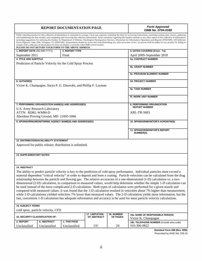
The ability to predict particle velocity is key to the prediction of cold spray performance. Individual particles must exceed a material dependent “critical velocity” in order to deposit and form a coating. Particle velocities can be calculated from the drag relationship between the particle and flowing gas. The relative accuracies of a one-dimensional (1-D) calculation vs. a two-dimensional (2-D) calculation, in comparison to measured values, would help determine whether the simple 1-D calculation can be used instead of the more complicated 2-D calculation. Both types of calculation were performed for a given nozzle and compared with measured values. It was found that the 1-D calculation resulted in velocities about 7% higher than measurement, while 2-D calculations yielded velocities 7% lower than measured values. The 2-D calculation yields more information, but the fast, convenient 1-D calculation has adequate information and accuracy to be used for most particle velocity calculations. 15. SUBJECT TERMS

cold spray, particle velocity, CFD

16. SECURITY CLASSIFICATION OF: 17. LIMITATION OF ABSTRACT

UU

18. NUMBER OF PAGES

24

19a. NAME OF RESPONSIBLE PERSON

Victor K. Champagne a. REPORT

Unclassified b. ABSTRACT

Unclassified c. THIS PAGE

Unclassified 19b. TELEPHONE NUMBER (Include area code)

410-306-0822 Standard Form 298 (Rev. 8/98)

Prescribed by ANSI Std. Z39.18

iii

Contents

List of Figures iv 

List of Tables iv 

1.  Introduction 1 

2.  Assumptions and Procedures 2 

2.1  Computational Modeling of the Nozzle ..........................................................................4 

2.2  Equation Set and Problem Setup in CFD++ ....................................................................4 

2.3  Computational Grid .........................................................................................................5 

2.4  Boundary Conditions .......................................................................................................5 

2.5  One-Dimensional Model .................................................................................................6 

2.6  Gas Flow..........................................................................................................................6 

2.7  Particle Motion ................................................................................................................7 

2.8  The 1-D Boundary and Initial Conditions .......................................................................7 

2.9  Experimental Arrangement .............................................................................................7 

3.  Results and Discussion 8 

3.1  Model Calculations – Full Nozzle Length ......................................................................8 

3.2  Model Comparison With Experiment ...........................................................................10 

4.  Conclusions 12 

5.  References 14 

Distribution List 16

iv

List of Figures

Figure 1. The cold spray process. ...................................................................................................1 

Figure 2. H-12 aluminum powder. ..................................................................................................3 

Figure 3. Aluminum H-12 deposit over 6061 aluminum alloy. ......................................................3 

Figure 4. Nozzle geometry (not to scale). .......................................................................................4 

Figure 5. The grid construction. ......................................................................................................5 

Figure 6. DPV 2000 operating principle. ........................................................................................8 

Figure 7. The 1-D and axisymmetric calculated results. ................................................................9 

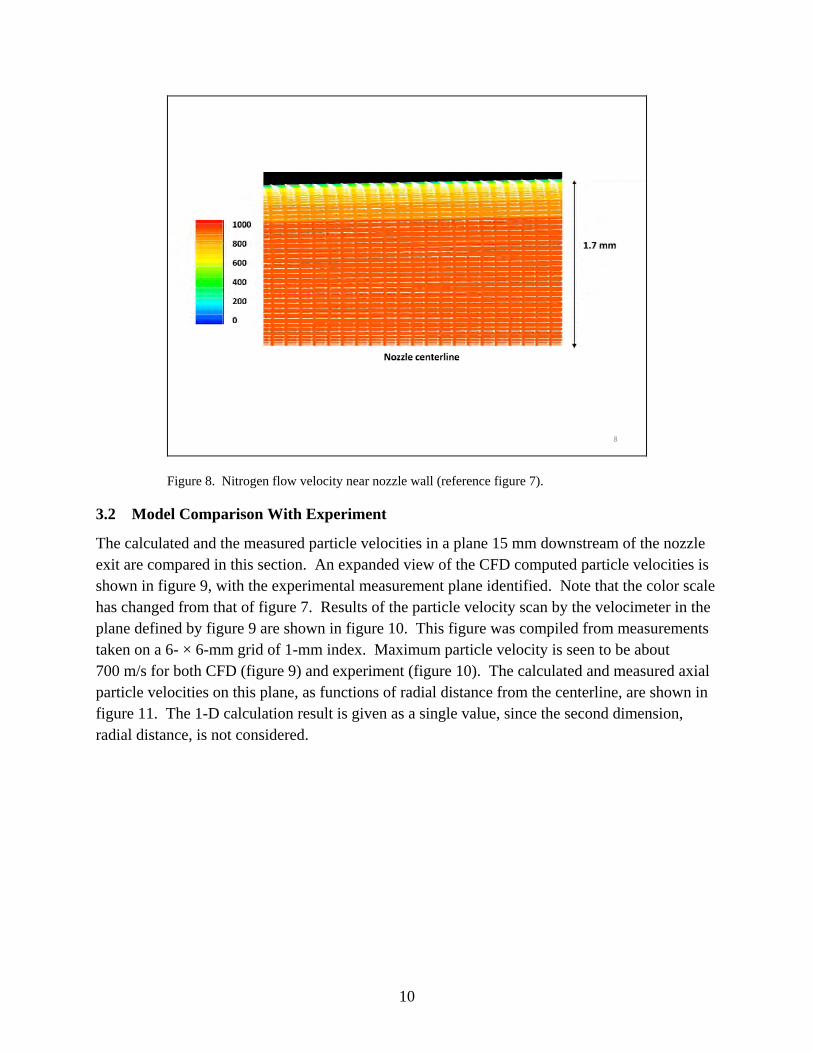
Figure 8. Nitrogen flow velocity near nozzle wall (reference figure 7). ......................................10 

Figure 9. The CFD-calculated exit plume of the nozzle. ..............................................................11 

Figure 10. Particle-velocity measurement in the exit plume. .......................................................11 

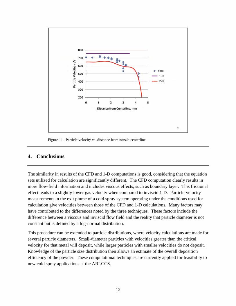
Figure 11. Particle velocity vs. distance from nozzle centerline. .................................................12 

List of Tables

Table 1. Boundary conditions. ........................................................................................................6 

1

1. Introduction

Coatings are often crucial for the strengthening or protection of vulnerable substrates. The quality of these coatings is characterized by the non-porous nature of the coating and its ability to adhere to the substrate. Extremely non-porous and adherent metallic as well as non-metallic coatings can be applied to surfaces by impacting suitable particles onto the surface at supersonic velocities. This cold spray process is carried out at the U.S. Army Research Laboratory Center for Cold Spray (ARLCCS) in Aberdeen, MD.

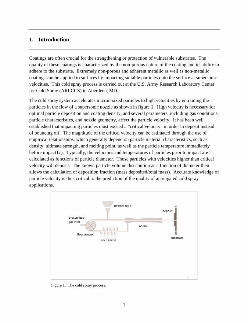
The cold spray system accelerates micron-sized particles to high velocities by entraining the particles in the flow of a supersonic nozzle as shown in figure 1. High velocity is necessary for optimal particle deposition and coating density, and several parameters, including gas conditions, particle characteristics, and nozzle geometry, affect the particle velocity. It has been well established that impacting particles must exceed a “critical velocity” in order to deposit instead of bouncing off. The magnitude of the critical velocity can be estimated through the use of empirical relationships, which generally depend on particle material characteristics, such as density, ultimate strength, and melting point, as well as the particle temperature immediately before impact (1). Typically, the velocities and temperatures of particles prior to impact are calculated as functions of particle diameter. Those particles with velocities higher than critical velocity will deposit. The known particle volume distribution as a function of diameter then allows the calculation of deposition fraction (mass deposited/total mass). Accurate knowledge of particle velocity is thus critical to the prediction of the quality of anticipated cold spray applications.

1

Figure 1. The cold spray process.

2

Particle velocity can be calculated and can be measured directly. Both techniques are non-trivial and require complex calculation and equipment. The U.S. Army has utilized one-dimensional (1-D), frictionless, gas-dynamic calculations in order to predict gas flow velocities for various cold spray operating conditions (2). Li and Li (3) make use of commercial computational fluid dynamics (CFD) code to optimize nozzle geometry for maximum particle velocity. Pardhasaradhi et al. (4) compare laser illuminated, time of flight velocity measurements with the empirical model given by Alkhimov et al. (5). Jodoin et al. (6) utilize the Reynolds average Navier Stokes equations within a computational platform to model nozzle flow with boundary conditions similar to those employed here, and they document the effects of gas type and stagnation conditions. Samareh et al. (7) use computational fluid mechanics to describe the effect of particle concentration on gas velocity for two nozzle geometries. Both Jodoin et al. and Samareh et al. compare calculation to measurement by means of time-of-flight between pulsed illumination.

A concern at the U.S. Army Research Laboratory (ARL) has centered about the magnitude of overestimation of particle velocity and hence deposition efficiency due to the neglect of friction and boundary layer effects in the 1-D calculation. This concern initiated efforts to enhance the modeling through the addition of friction via CFD. Accordingly, an effort was initiated to determine the scope of variation among methods of particle velocity prediction and measurement.

2. Assumptions and Procedures

Deposition of aluminum by cold spray is a common application and is often applied for the purpose of substrate corrosion protection and for defect repair. A Ktech (Albuquerque, NM) cold spray system was used by ARL to deposit aluminum. The arrangement of this system is described by figure 1, and is very similar to cold spray systems operated in other facilities. The particle velocities at the nozzle exit of this specific cold spray system and nozzle are considered here.

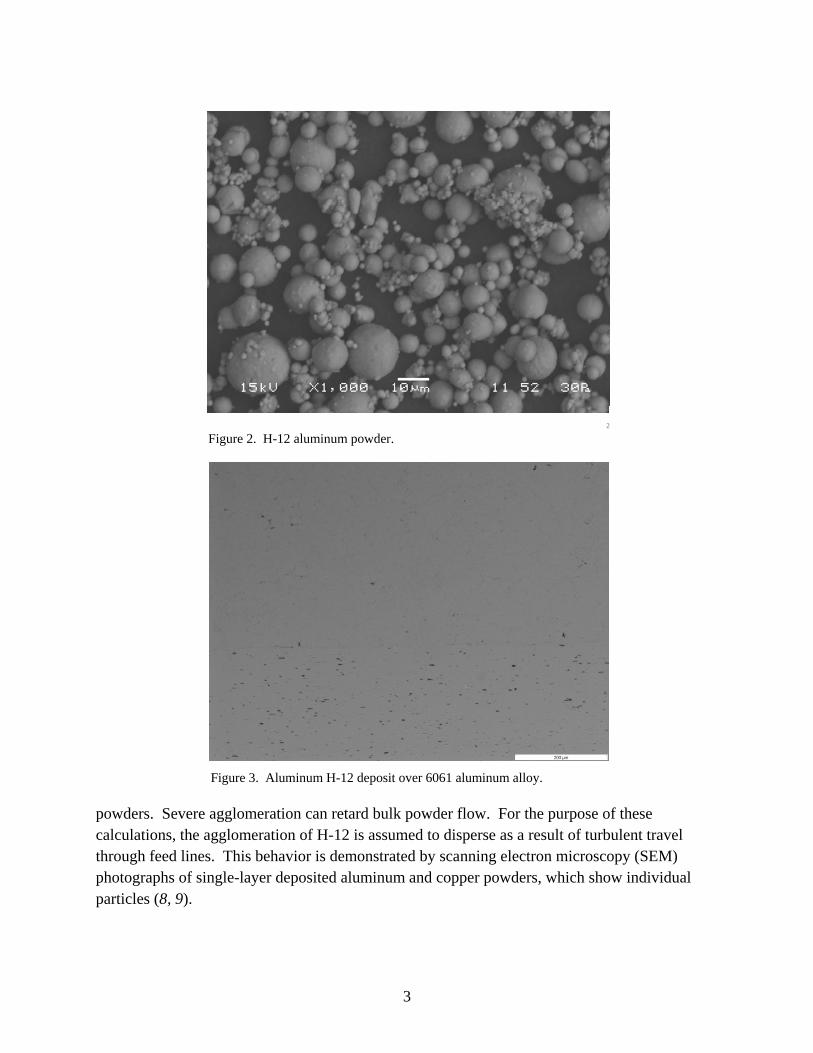
The aluminum powder used for these calculations and experiments is identified as H-12, supplied by Valimet Inc. (Stockton, CA). The powder has a lognormal distribution with a mean diameter of 15 µm and a standard deviation of 1.57. A micrograph of this powder is shown in figure 2, and it is seen that all particles are spherical. The resulting deposition of this powder when cold sprayed under the conditions of this report is shown in figure 3.

The calculations described here consider spherical, 15-µm-diameter particles only. Non-spherical particles can be considered if a form factor adjustment is made to the coefficient of drag. Particle agglomeration, as can be seen in figure 3, is generally found for all thermal spray

3

2 Figure 2. H-12 aluminum powder.

Figure 3. Aluminum H-12 deposit over 6061 aluminum alloy.

powders. Severe agglomeration can retard bulk powder flow. For the purpose of these calculations, the agglomeration of H-12 is assumed to disperse as a result of turbulent travel through feed lines. This behavior is demonstrated by scanning electron microscopy (SEM) photographs of single-layer deposited aluminum and copper powders, which show individual particles (8, 9).

4

2.1 Computational Modeling of the Nozzle

The commercially available software GridPro, for generating curvilinear grids, and CFD++, for solving the flow (Metacomp Technologies, Agoura Hills, CA), were selected for the axi-symmetric flow solution. A two-dimensional (2-D) grid was generated using GridPro and the axi-symmetric option was used in CFD++ to simulate the flow through the nozzle. The entire nozzle geometry is shown in figure 4 to give a general idea of the dimensions involved. The nozzle throat diameter is 2 mm and the exit diameter is 7 mm, for an area ratio of 12.25. The length of the nozzle as modeled was 153 mm, beginning at the particle injection point and ending at the nozzle exit.

4

Figure 4. Nozzle geometry (not to scale).

2.2 Equation Set and Problem Setup in CFD++

The Reynolds Averaged Navier Stokes equation set, along with the realizable k-ε turbulence model for the fluid, was selected as governing. This gave a total of six equations—conservation of mass, conservation of momentum in 2-D, conservation of energy, an equation for the turbulent kinetic energy, k, and an equation for turbulence dissipation, ε.

CFD++ uses the Eulerian Dispersed Phase model to couple the dispersed phase with the fluid dynamics. For the dispersed species, an additional three equations must be solved. These are the mass equation and the momentum equations in two directions. In addition to the interphase drag force, the effects of pressure gradient force, the virtual-mass force, lift force, and the turbulent dispersion force have been included. The effect of gravity was not included due to the small particle size (15-µm diameter) and the high speeds (Mach 1–3) involved. A Eulerian-based Henderson drag coefficient model was used for the gas-particle flow interactions (10).

5

2.3 Computational Grid

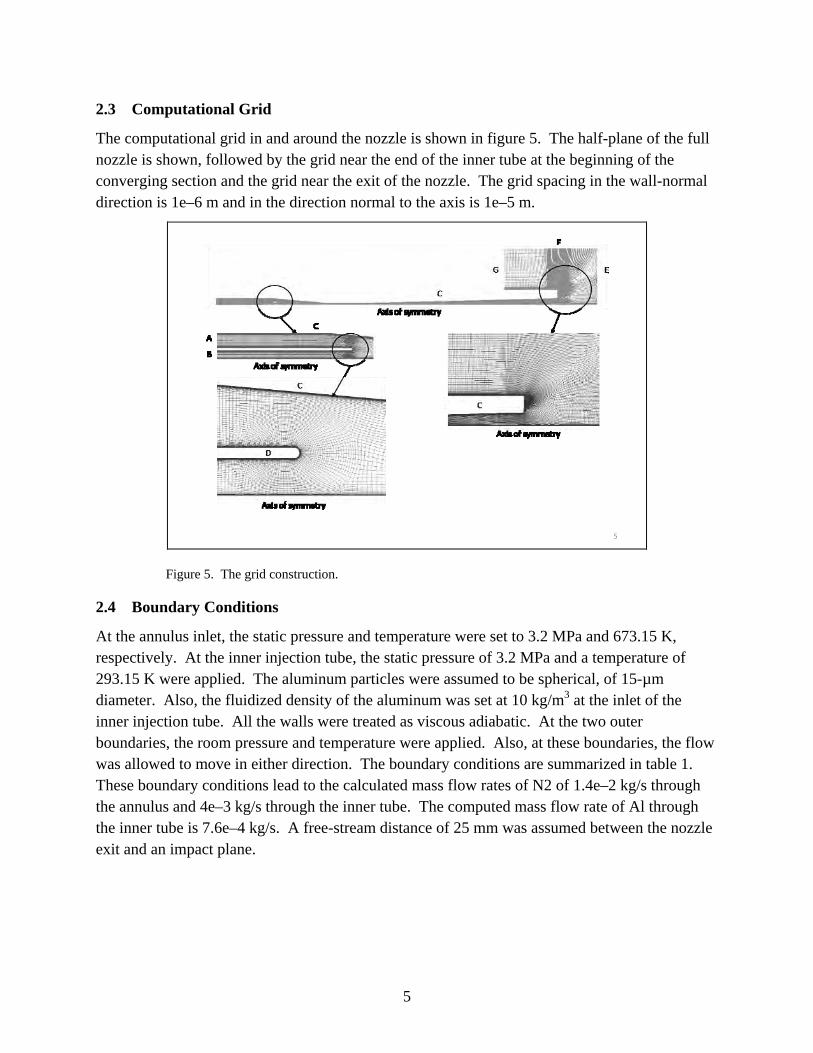
The computational grid in and around the nozzle is shown in figure 5. The half-plane of the full nozzle is shown, followed by the grid near the end of the inner tube at the beginning of the converging section and the grid near the exit of the nozzle. The grid spacing in the wall-normal direction is 1e–6 m and in the direction normal to the axis is 1e–5 m.

5

Figure 5. The grid construction.

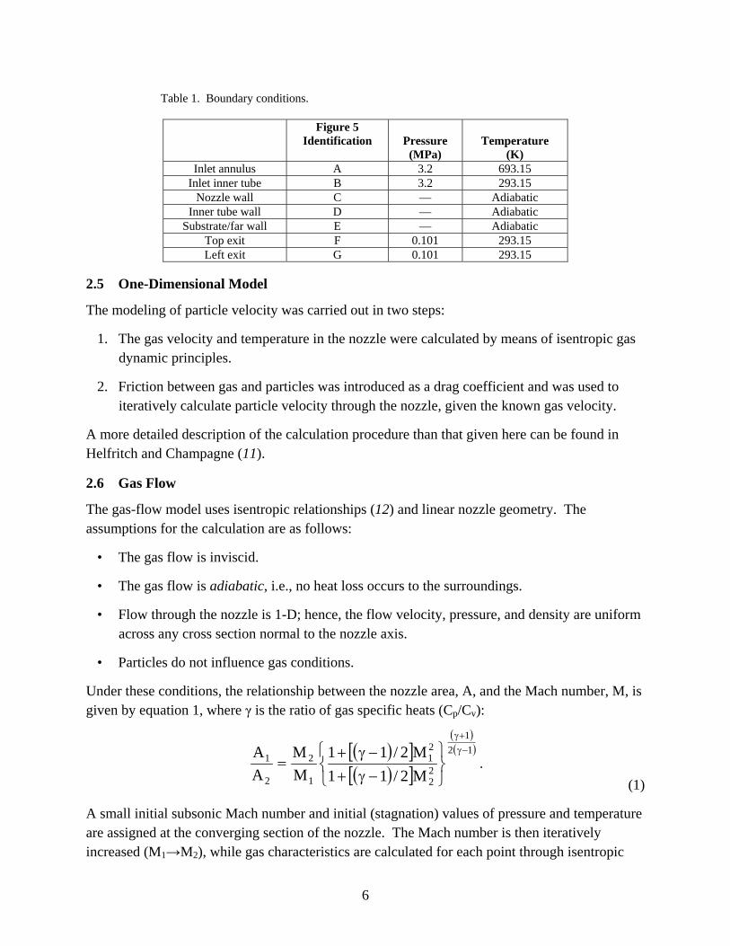
2.4 Boundary Conditions

At the annulus inlet, the static pressure and temperature were set to 3.2 MPa and 673.15 K, respectively. At the inner injection tube, the static pressure of 3.2 MPa and a temperature of 293.15 K were applied. The aluminum particles were assumed to be spherical, of 15-µm diameter. Also, the fluidized density of the aluminum was set at 10 kg/m3 at the inlet of the inner injection tube. All the walls were treated as viscous adiabatic. At the two outer boundaries, the room pressure and temperature were applied. Also, at these boundaries, the flow was allowed to move in either direction. The boundary conditions are summarized in table 1. These boundary conditions lead to the calculated mass flow rates of N2 of 1.4e–2 kg/s through the annulus and 4e–3 kg/s through the inner tube. The computed mass flow rate of Al through the inner tube is 7.6e–4 kg/s. A free-stream distance of 25 mm was assumed between the nozzle exit and an impact plane.

6

Table 1. Boundary conditions.

Figure 5

Identification

Pressure (MPa)

Temperature (K)

Inlet annulus A 3.2 693.15 Inlet inner tube B 3.2 293.15

Nozzle wall C — Adiabatic Inner tube wall D — Adiabatic

Substrate/far wall E — Adiabatic Top exit F 0.101 293.15 Left exit G 0.101 293.15

2.5 One-Dimensional Model

The modeling of particle velocity was carried out in two steps:

1. The gas velocity and temperature in the nozzle were calculated by means of isentropic gas dynamic principles.

2. Friction between gas and particles was introduced as a drag coefficient and was used to iteratively calculate particle velocity through the nozzle, given the known gas velocity.

A more detailed description of the calculation procedure than that given here can be found in Helfritch and Champagne (11).

2.6 Gas Flow

The gas-flow model uses isentropic relationships (12) and linear nozzle geometry. The assumptions for the calculation are as follows:

• The gas flow is inviscid.

• The gas flow is adiabatic, i.e., no heat loss occurs to the surroundings.

• Flow through the nozzle is 1-D; hence, the flow velocity, pressure, and density are uniform across any cross section normal to the nozzle axis.

• Particles do not influence gas conditions.

Under these conditions, the relationship between the nozzle area, A, and the Mach number, M, is given by equation 1, where γ is the ratio of gas specific heats (Cp/Cv):

12

1

22

21

1

2

2

1

M2/11

M2/11

M

M

A

A

.

(1)

A small initial subsonic Mach number and initial (stagnation) values of pressure and temperature are assigned at the converging section of the nozzle. The Mach number is then iteratively increased (M1→M2), while gas characteristics are calculated for each point through isentropic

7

relationships. Equation 1 yields the change in area (A1→A2) required for the Mach number increment, and progression along the nozzle axis is calculated from the area change and the nozzle geometry given by figure 4. The Mach number is increased past Mach 1 until the calculated longitudinal magnitude exceeds the nozzle length. This results in the initial, assigned Mach number at the nozzle entrance, Mach 1 at the nozzle minimum area, or throat, and approximately Mach 3 at the nozzle exit.

2.7 Particle Motion

Once the gas conditions and velocity were characterized, the particle velocity was iteratively calculated from the nozzle entrance to the substrate through the use of the particle drag relationship, given by equation 2.

228/ pggD

pVVdC

dt

dVm ,

(2)

where Vp and Vg are particle and gas velocities, m is the particle mass, ρg is the gas density, and d is the particle diameter. The drag coefficient, CD, is given by Carlson and Hoglund (13), who correct the simple Stokes drag law relationship for inertial, compressibility, and rarefaction effects.

2.8 The 1-D Boundary and Initial Conditions

The nozzle shape, i.e., radius vs. distance from the inlet, was chosen to be equal to that used for the CFD computation, as shown in figure 4. The stagnation pressure was assumed to be 3.2 MPa, as given in table 1. The stagnation temperature was assumed to be 588 K, which corresponds to the mixed temperature of the inlet annulus and inlet inner tube of table 1. The aluminum particle characteristics were equal to that of the CFD computation, i.e., spherical, 15-µm diameter.

2.9 Experimental Arrangement

A cold spray system at ARL was used to generate the data herein. This system is described in more detail by Champagne et al. (14). The nozzle geometry of this system is given by figure 4. Aluminum powder with a particle volume mean diameter of 15 µm was sprayed, while the system was operated at the pressures and temperatures given by table 1.

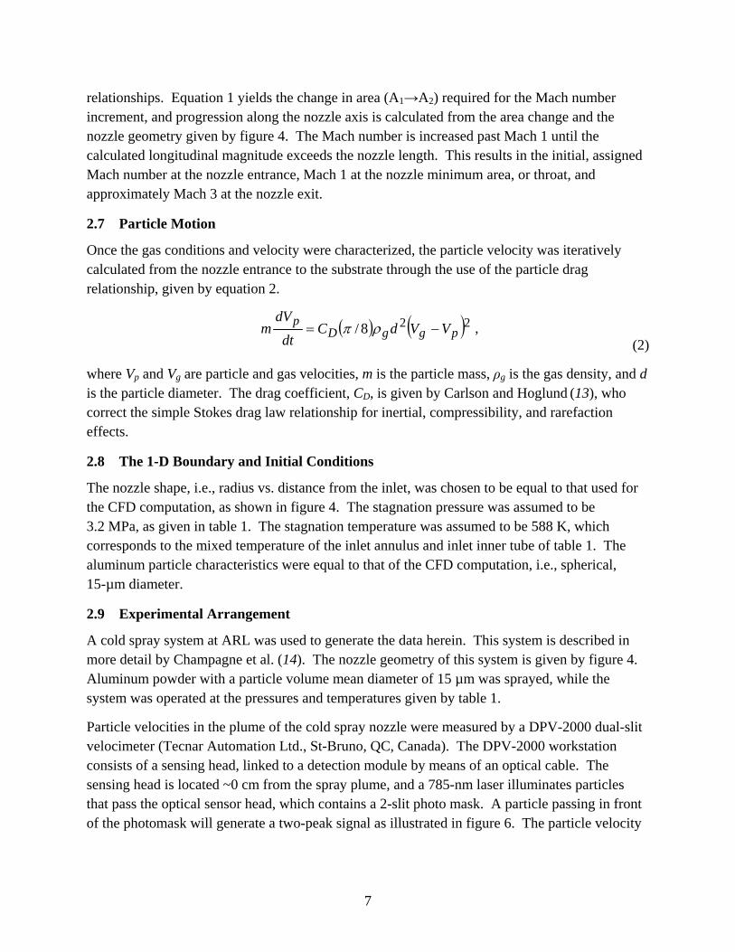
Particle velocities in the plume of the cold spray nozzle were measured by a DPV-2000 dual-slit velocimeter (Tecnar Automation Ltd., St-Bruno, QC, Canada). The DPV-2000 workstation consists of a sensing head, linked to a detection module by means of an optical cable. The sensing head is located ~0 cm from the spray plume, and a 785-nm laser illuminates particles that pass the optical sensor head, which contains a 2-slit photo mask. A particle passing in front of the photomask will generate a two-peak signal as illustrated in figure 6. The particle velocity

8

6

Figure 6. DPV 2000 operating principle.

is the time of flight between the slits, divided by the distance between the slits. The sensing head is mechanically scanned such that the focus point defines a 6- × 6-mm grid of 1-mm mesh size in a plane perpendicular to the plume.

The velocities of all particles are measured, and averaged values of these measurements at each mesh point comprise the recorded velocity at that point. The Cartesian coordinates are then converted to cylindrical in order to compare with calculation

3. Results and Discussion

3.1 Model Calculations – Full Nozzle Length

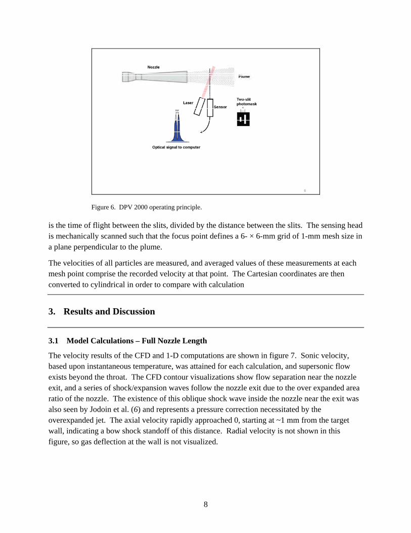
The velocity results of the CFD and 1-D computations are shown in figure 7. Sonic velocity, based upon instantaneous temperature, was attained for each calculation, and supersonic flow exists beyond the throat. The CFD contour visualizations show flow separation near the nozzle exit, and a series of shock/expansion waves follow the nozzle exit due to the over expanded area ratio of the nozzle. The existence of this oblique shock wave inside the nozzle near the exit was also seen by Jodoin et al. (6) and represents a pressure correction necessitated by the overexpanded jet. The axial velocity rapidly approached 0, starting at ~1 mm from the target wall, indicating a bow shock standoff of this distance. Radial velocity is not shown in this figure, so gas deflection at the wall is not visualized.

9

7

Figure 7. The 1-D and axisymmetric calculated results.

Particles are uniformly accelerated by the gas flow. They are relatively unaffected by the extreme variations in gas velocity at the nozzle exit, due to the momentum of the particles. Unlike the gas, the axial particle velocity remains high to the point of boundary impact.

The axial CFD-computed velocities and 1-D results are compared in the graph of figure 7, where the x scale corresponds to the nozzle visualizations above. Large variations in gas velocity due to shock and expansion waves are seen at the nozzle exit for the CFD calculation. This effect is not captured by the 1-D analysis. The 1-D computation yields gas and particle velocities that are ~100 m/s higher than that of the CFD computation at the nozzle exit. This difference can be attributed to the inviscid assumption of the 1-D calculation.

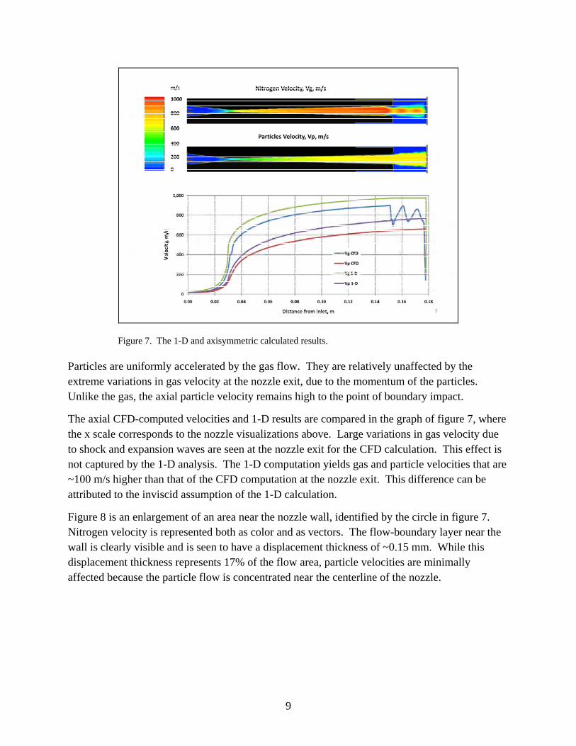
Figure 8 is an enlargement of an area near the nozzle wall, identified by the circle in figure 7. Nitrogen velocity is represented both as color and as vectors. The flow-boundary layer near the wall is clearly visible and is seen to have a displacement thickness of ~0.15 mm. While this displacement thickness represents 17% of the flow area, particle velocities are minimally affected because the particle flow is concentrated near the centerline of the nozzle.

10

8

Figure 8. Nitrogen flow velocity near nozzle wall (reference figure 7).

3.2 Model Comparison With Experiment

The calculated and the measured particle velocities in a plane 15 mm downstream of the nozzle exit are compared in this section. An expanded view of the CFD computed particle velocities is shown in figure 9, with the experimental measurement plane identified. Note that the color scale has changed from that of figure 7. Results of the particle velocity scan by the velocimeter in the plane defined by figure 9 are shown in figure 10. This figure was compiled from measurements taken on a 6- × 6-mm grid of 1-mm index. Maximum particle velocity is seen to be about 700 m/s for both CFD (figure 9) and experiment (figure 10). The calculated and measured axial particle velocities on this plane, as functions of radial distance from the centerline, are shown in figure 11. The 1-D calculation result is given as a single value, since the second dimension, radial distance, is not considered.

11

9

Figure 9. The CFD-calculated exit plume of the nozzle.

Horizontal, mm

-3 -2 -1 0 1 2 3

Ver

tica

l, m

m

-3

-2

-1

0

1

2

3

475 500 525 550 575 600 625 650 675 700 725

10

Figure 10. Particle-velocity measurement in the exit plume.

12

11

Figure 11. Particle velocity vs. distance from nozzle centerline.

4. Conclusions

The similarity in results of the CFD and 1-D computations is good, considering that the equation sets utilized for calculation are significantly different. The CFD computation clearly results in more flow-field information and includes viscous effects, such as boundary layer. This frictional effect leads to a slightly lower gas velocity when compared to inviscid 1-D. Particle-velocity measurements in the exit plume of a cold spray system operating under the conditions used for calculation give velocities between those of the CFD and 1-D calculations. Many factors may have contributed to the differences noted by the three techniques. These factors include the difference between a viscous and inviscid flow field and the reality that particle diameter is not constant but is defined by a log-normal distribution.

This procedure can be extended to particle distributions, where velocity calculations are made for several particle diameters. Small-diameter particles with velocities greater than the critical velocity for that metal will deposit, while larger particles with smaller velocities do not deposit. Knowledge of the particle size distribution then allows an estimate of the overall deposition efficiency of the powder. These computational techniques are currently applied for feasibility to new cold spray applications at the ARLCCS.

13

The computations show particle impact velocities above 650 m/s. The ARLCCS has shown that aluminum deposition results when operating the nozzle at the initial conditions chosen for these computations. It is also known that velocities below the critical value of ~600 m/s do not result in aluminum deposition (1). The computational results are thus verified by known aluminum particle deposition by cold spray.

14

5. References

1. Schmidt, T.; Gartner, F.; Assadi, H.; Kreye, H. Development of a Generalized Parameter Window for Cold Spray Deposition. Acta Materialia 2006, 54, 729–742.

2. Champagne, V. K.; Helfritch, D. J.; Leyman, P. F.; Lempicki, R.; Grendahl, S. The Effects of Gas and Metal Characteristics on Sprayed Metal Coatings, Modeling. Simul. Mater. Sci. Eng., 2005, 13, 1–10.

3. Li, W.; Li, C. Optimal Design of a Novel Cold Spray Gun Nozzle at a Limited Space. J. of Thermal Spray Technology 2005, 14 (3), 391–396.

4. Pardhasaradhi, S. P.; Venkatachalapathy, V.; Joshi, S. V.; Govindanet, S. Optical Diagnostics Study of Gas Particle Transport Phenomena in Cold Gas Dynamic Spraying and Comparison with Model Predictions. J. of Thermal Spray Technology 2008, 17 (4) 551–563.

5. Alkhimov, A. P.; Kosarev, V. F.; Klinkov, S. V. The Features of Cold Spray Nozzle Design, J. Thermal Spray Technology, 2001, 10 (2), 375–381.

6. Jodoin, B.; Raletz, F.; Vardelle, M. Cold Spray Modeling and Validation Using an Optical Diagnostic Method. Surface & Coatings Technology, 2006, 200, 4424–4432.

7. Samareh, B.; Stier, O.; Luthen, V.; Dolatabadi, A. Assessment of CFD Modeling via Flow Visualization in Cold Spray Process. J. Thermal Spray Technol., published online 2009.

8. Guetta, S.; Berger, M.; Borit, F.; Guipont, V.; Jeandin, M.; Boustie, M.; Ichikawa, Y.; Sagaguchi, K.; Ogawa, K. Influence of Particle Velocity on Adhesion of Cold-Sprayed Splats. J. of Thermal Spray Technology, 2009, 18 (3) 331–342.

9. King, P.; Jahedi, M. Relationship Between Particle Size and Deformation in the Cold Spray Process. Applied Surface Science, 2010, 256, 1735–1738.

10. Henderson, C. Drag Coefficients of Spheres in Continuum and Rarefied Flows. AIAA Journal, 1976, 14 (6), 707–8.

11. Helfritch, D. J.; Champagne, V. K. Optimal Particle Size for the Cold Spray Process, Proceedings of the International Thermal Spray Conference, Seattle, WA, May, 2006

12. Shapiro, A. The Dynamic and Thermodynamics of Compressible Fluid Flow; Roland Press: New York, NY, 1953; p 73–94.

15

13. Carlson, D.; Hoglund, R. Particle Drag and Heat Transfer in Rocket Nozzles. AIAA Journal, 2 (11), 1980–1984.

14. Champagne, V. K.; Helfritch, D. J.; Leyman, P. F.; Grendahl, S.; Klotz, B. Interface Material Mixing Formed by the Deposition of Copper on Aluminum by Means of the Cold Spray Process. J. of Thermal Spray Technology 2005, 14 (3) 330–334.

NO. OF COPIES ORGANIZATION

16

1 DEFENSE TECHNICAL (PDF INFORMATION CTR only) DTIC OCA 8725 JOHN J KINGMAN RD STE 0944 FORT BELVOIR VA 22060-6218 1 DIRECTOR US ARMY RESEARCH LAB IMNE ALC HRR 2800 POWDER MILL RD ADELPHI MD 20783-1197 1 DIRECTOR US ARMY RESEARCH LAB RDRL CIO LL 2800 POWDER MILL RD ADELPHI MD 20783-1197 1 DIRECTOR US ARMY RESEARCH LAB RDRL CIO MT 2800 POWDER MILL RD ADELPHI MD 20783-1197 1 DIRECTOR US ARMY RESEARCH LAB RDRL D 2800 POWDER MILL RD ADELPHI MD 20783-1197

NO. OF COPIES ORGANIZATION

17

ABERDEEN PROVING GROUND 10 DIR USARL RDRL WMM D V CHAMPAGNE (5 CPS) D HELFRITCH (5 CPS)

18

INTENTIONALLY LEFT BLANK.