Vol:.(1234567890)

Petroleum Science (2019) 16:1086–1104https://doi.org/10.1007/s12182-019-0342-6

1 3

ORIGINAL PAPER

Prediction of immiscible gas flooding performance: a modified capacitance–resistance model and sensitivity analysis

Seyed Hamidreza Yousefi1 · Fariborz Rashidi2 · Mohammad Sharifi1 · Mohammad Soroush3

Received: 18 July 2018 / Published online: 9 July 2019 © The Author(s) 2019

AbstractReservoir performance prediction is one of the main steps during a field development plan. Due to the complexity and time-consuming aspects of numerical simulators, it is helpful to develop analytical tools for a rapid primary analysis. The capacitance–resistance model (CRM) is a simple technique for reservoir management and optimization. This method is an advanced time-dependent material balance equation which is combined with a productivity equation. CRM uses production/injection data and bottom-hole pressure as inputs to build a reliable model, which is then combined with the oil-cut model and converted to a predictive tool. CRM has been studied thoroughly for water flooding projects. In this study, a modified model for gas flooding systems based on gas density and average reservoir pressure is developed. A detailed procedure is described in a synthetic reservoir model using a genetic algorithm. Then, a streamline simulation is implemented for validation of the results. The results show that the proposed model is able to calculate interwell connectivity parameters and oil production rates. Moreover, a sensitivity analysis is carried out to investigate effects of drawdown pressure and gas PVT properties on the new model. Finally, acceptable ranges of input data and limitations of the model are comprehensively discussed.

Keywords Reservoir management · Capacitance–resistance model · Gas flooding · Analytical model · Sensitivity analysis · Streamline simulation

1 Introduction

Gas flooding in reservoirs is a well-known secondary recov-ery mechanism and also a gas storage method in the world (Bybee 2001; Azin et al. 2008; Mohammadi et al. 2011; Yuncong et al. 2014; Agrawal et al. 2016; Kumar et al. 2017). Comprehensive analysis of miscible/immiscible gas injection has been undertaken by many researchers using laboratory tests and numerical modeling (Kulkarni and

Rao 2005; Alkhazmi et al. 2017; Rezaei et al. 2018). Many aspects of gas injection such as production mechanisms and practical field implementation have also been reviewed (Miri et al. 2014; Agrawal et al. 2016; Kostelnik et al. 2017). Field management and optimization in the gas injection process are important tasks in a reservoir life cycle. Commercial numerical simulators are commonly used for these pur-poses. Detailed input data including gridding, petrophysics, pressure–temperature–volume (PVT), special core analysis (SCAL), initialization and well data are required for simula-tion. Comprehensive analysis of reservoir performance, such as well placement optimization and enhanced oil recovery (EOR) scenario prediction, should be performed by numeri-cal methods. However, numerical solution methods based on finite difference or finite element schemes are compu-tationally expensive and time-consuming. Thus, analytical and semi-analytical approaches are necessary for primary analysis for a field development plan. The main advantages of analytical tools are low computational time, simplicity and limited number of input data compared to numerical simulation methods.

Edited by Yan-Hua Sun

* Fariborz Rashidi rashidi@aut.ac.ir

Seyed Hamidreza Yousefi s.h.yousefi@aut.ac.ir

1 Department of Petroleum Engineering, Amirkabir University of Technology, Tehran, Iran

2 Department of Chemical Engineering, Amirkabir University of Technology, Tehran, Iran

3 Petroleum Engineering Department, University of Trinidad and Tobago, Couva, Trinidad and Tobago

1087Petroleum Science (2019) 16:1086–1104

1 3

Analytical methods stand between simple tools (the graphical methods and the decline curve analysis) and com-mercial numerical simulators. CRM is an analytical tool that considers a reservoir as a tank and its formulation is based on the material balance equation between the input (injection rate) and output (production rate) data in a specific control volume (Fig. 1). CRM only requires available and reliable data including production rate, injection rate and producers’ BHP. This method is inspired from electrical engineering in which fluid flow, porous media storativity, pressure depletion and permeability can be conceptually substituted for elec-tric current, capacitance, electric potential and resistance, respectively. The main unknowns in the CRM are interwell connectivity (f) and the time constant (τ). The well produc-tion rate in CRM is a function of injection rate, interwell connectivity, time constant and BHP.

Interwell connectivity is an essential parameter in res-ervoir management which can affect well rate allocation, infill drilling and sweep efficiency optimization. Interwell connectivity shows the injector contribution in the produc-tion of surrounding producers and is a function of reser-voir geometry, degree of heterogeneity and well distances. It is also useful for identification of flow barriers as well as high-permeability channels between the injector and the producer (Rafiei 2014). This parameter can be deter-mined using CRM or other direct and indirect methods. Direct methods such as 4D seismic (Huang and Ling 2006; Huseby et al. 2008; Yin et al. 2015, 2016), pulse testing (Dinges and Ogbe 1988; Fokker et al. 2012), interference (Al-Khamis et al. 2005; Ogbe and Brigham 1989; Stewart and Gupta 1984) well tests and tracer tests (Du and Guan 2005; Dugstad et al. 1999; Huseby et al. 2008; Lichten-berger 1991; Refunjol and Lake 1999) are operationally implemented in the field. Although indirect methods are data-driven models and are based on input–output signals

which are developed mathematically or statistically, they include artificial neural networks (ANN) (Demiryurek et al. 2008; Panda and Chopra 1998; Artun 2017), wave-let analysis (Jansen and Kelkar 1997), Spearman rank correlation (Heffer et al. 1997; Fedenczuk and Hoffmann 1998; Refunjol and Lake 1999), extended Kalman filter (Liu et al. 2009), pressure-based method (Dinh and Tiab 2008), multiwell productivity method (Valko et al. 2000; Kaviani and Valkó 2010), network model (Gherabati et al. 2017a, b), and streamline simulation (SS) (Batycky et al. 1997, 2005; Thiele et al. 2010; Thiele and Batycky 2006; Baker 2001).

The time constant shows the time needed for transferring the response signal from the injector to the producer (Cao et al. 2014). This parameter is a representative of the fluid storage between injector and producer (Soroush et al. 2014). A low time constant shows a high impact of the injection rate on the production response (Sayarpour et al. 2007). This parameter is a function of total compressibility, productiv-ity index (PI) and pore volume. Generally, a well pair with low interwell connectivity has a large time constant (Cao et al. 2014).

Using historical data, CRM predicts total (oil, gas and water) well production rate. Then, by coupling CRM with oil-cut models such as the Gentil model (Gentil 2005) or the Koval model (Koval 1963), oil, gas and water rates of the well can be estimated.

The main assumptions of the CRM formulation are:

• Constant PI• Constant temperature• Low-compressible and immiscible fluids• Darcy law flow• Constant operational conditions

I2

Time Time

Inje

ctio

n ra

te I(t)

Pro

duct

ion

rate

q(t)

Input signal I(t) Output response q(t)

Arbitrary reservoir control volume

t0 t1 t2 t3 tn-1 tn t0 t1 t2 t3 tn-1 tn

I4In

In-1

I3

I1

Fig. 1 CRM as a signal-based method—effect of input signal on output signal in a control volume (Sayarpour 2008)

1088 Petroleum Science (2019) 16:1086–1104

1 3

CRM covers a wide range of applications including res-ervoir management and optimization, interwell connectiv-ity characterization, heterogeneity identification and rate allocation optimization. Below we present a brief introduc-tion to CRM development, model improvements and its applications.

Mathematical formulation of the CRM was developed by Yousef et al. (Yousef et al. 2006, 2005). To derive this for-mulation, they coupled the linear productivity model and the material balance equation and defined a connectivity param-eter and time constant. Also, they developed a diagnostic tool for identification of flow barriers and transmissibility trends (Yousef et al. 2009). Then, mathematical equations for a system of three control volumes based on tank, pro-ducer and injector-producer, using superposition in time, were obtained by Sayarpour et al. (Sayarpour et al. 2007, 2009). Weber et al. (2009) coupled their CRM model with an optimizer and successfully tested the model in a field-scale scenario. Delshad et al. (2009) presented a new application of the CRM in characterization of fractures in the reservoir and quantitatively calculated the fracture permeability. Izgec and Kabir (2010) investigated the capability of the CRM in pre-breakthrough conditions in water flooding and validated the results by streamline simulation. Salazar-Bustamante et al. (2012) combined decline curve analysis and CRM in a carbonate reservoir under gas injection and developed an integrated model, which is applicable in reservoirs under pri-mary depletion and gas injection. Kaviani et al. (2012) intro-duced the segmented CRM where unknown BHPs change during the interval and compensated CRM in the case of adding a new producer or shutting in an existing producer. Kaviani et al. (2014) performed a comprehensive sensitivity analysis on the impact of different parameters on the CRM performance. They also defined a dimensionless number and with a specific range where CRM is applicable. Mamghaderi and Pourafshary (2013) improved the CRM for layered res-ervoirs by considering the crossflow between the layers and using available production logging tools (PLT) data. Moreno (2013) developed a multilayer CRM combined with a simple dynamic model and considered variable interwell connectiv-ity, as a function of time, using production and completion data. Moreno and Lake (2014a, b) investigated the impact of noise in the injection rate and designed input signals that improved the information from CRM to estimate interwell

connectivity. Also, they studied the uncertainty of interwell connectivity estimations from the CRM. Laochamroon-vorapongse et al. (2014) applied CRM for immiscible and miscible water alternating gas (WAG) floods and integrated CRM with other analytical tools such as a Hall plot and the reciprocal of the productivity index for better understand-ing of reservoir performance. Soroush et al. (2014) studied the effect of change in the producer’s skin factor, drilling new producers and shutting in active existing producers and developed a multiwell compensated capacitance model based on superposition. Cao et al. (2014) presented a two-phase CRM based on the total fluid and oil material balance equations. In addition to pressure changes, they included the saturation variations in the equations and showed that the modified CRM is able to estimate interwell connectivity in all time frames of water flooding. Tao and Bryant (Tao and Bryant 2015) used CRM for gas storage projects to identify connectivity between the extractor and the injector. They showed that CRM is very useful in poorly characterized stor-age aquifers. Eshraghi et al. (2016) employed CRM for CO2 miscible flooding combined with the Gentil fractional flow model. They further optimized CO2 flooding using heuris-tic methods such as GA and particle swarm optimization. Mirzayev and Jensen (2016) extended the CRM to a tight reservoir with high well densities and stimulation treatments by dividing the field to some small regions (windows) and considering pseudo wells. Zhang et al. (2017) developed multilayer CRM combined with the ensemble Kalman fil-ter for matching the parameters and performed production optimization by ensemble-based optimization. de Holanda et al. (2018) derived matrix representation of CRM using state space equations and used linear control algorithms for improvement of run-time in large fields. They successfully applied the model in a synthetic reservoir.

Most of the published literature on CRM is concentrated on water flooding projects. There are many gas flooding projects in the world, but comprehensive analysis of CRM performance on gas flooding projects has not been investi-gated and few published studies exist for gas flooding using the CRM. A list of these studies is provided in Table 1. The objective of this study is to extend the CRM equation in gas flooding systems. It should be noted that the original CRM was used in the studies shown in Table 1 for gas–oil systems. Low-compressible fluids (constant gas density) and

Table 1 Researches on the CRM applications in gas flooding

Researcher Description

Salazar-Bustamante et al. (2012) Combination of a decline curve model with the CRM in a fractured reservoir under a gas floodLaochamroonvorapongse et al. (2014) Interwell connectivity calculation in miscible and immiscible WAG floodsTao and Bryant (2015) Use of CRM for gas storage projects in an aquifer with CO2 injection and brine extractionEshraghi et al. (2016) Application of CRM in supercritical CO2 miscible injection using a heuristic optimization algorithm

1089Petroleum Science (2019) 16:1086–1104

1 3

linear productivity equation assumptions are not valid in gas flooding systems. In this study, a modified CRM based on compressible fluid consideration (variable density) and the Fetkovich productivity index is developed. To apply these modifications, inputs such as gas density and average res-ervoir pressure are required. Using this modified CRM, gas flooding projects can be analyzed with an acceptable range of accuracy for total well production rates, interwell param-eters and time constants. Then, the model is combined with one empirical fractional flow model to determine well oil and gas rate. Therefore, reservoir management and reservoir performance prediction in gas–oil systems can be performed using the modified CRM and the fractional flow model. Interwell connectivities and well rates are validated using a precise streamline simulator. Statistical error analysis shows that M-CRM results are in good agreement with SS.

2 Modified CRM

The modified CRM (M-CRM) is proposed as an analytical solution in gas–oil systems. The M-CRM is a combination of a modified mass balance equation and a modified produc-tivity equation. There are two approaches for considering gas–oil flow in the reservoir. The first one is based on Cao et al.’s studies (Cao et al. 2014). In this method, saturation changes are imported in the equations, and thus, it is nec-essary to solve pressure and saturation equations simulta-neously. This method is sophisticated and time-consuming when compared to the common CRM. The second one is the Izgec and Kabir approach (Izgec and Kabir 2010), in which they only modified the material balance equation by including density variation in the model. Since the CRM is required to remain simple and fast, we chose the second approach.

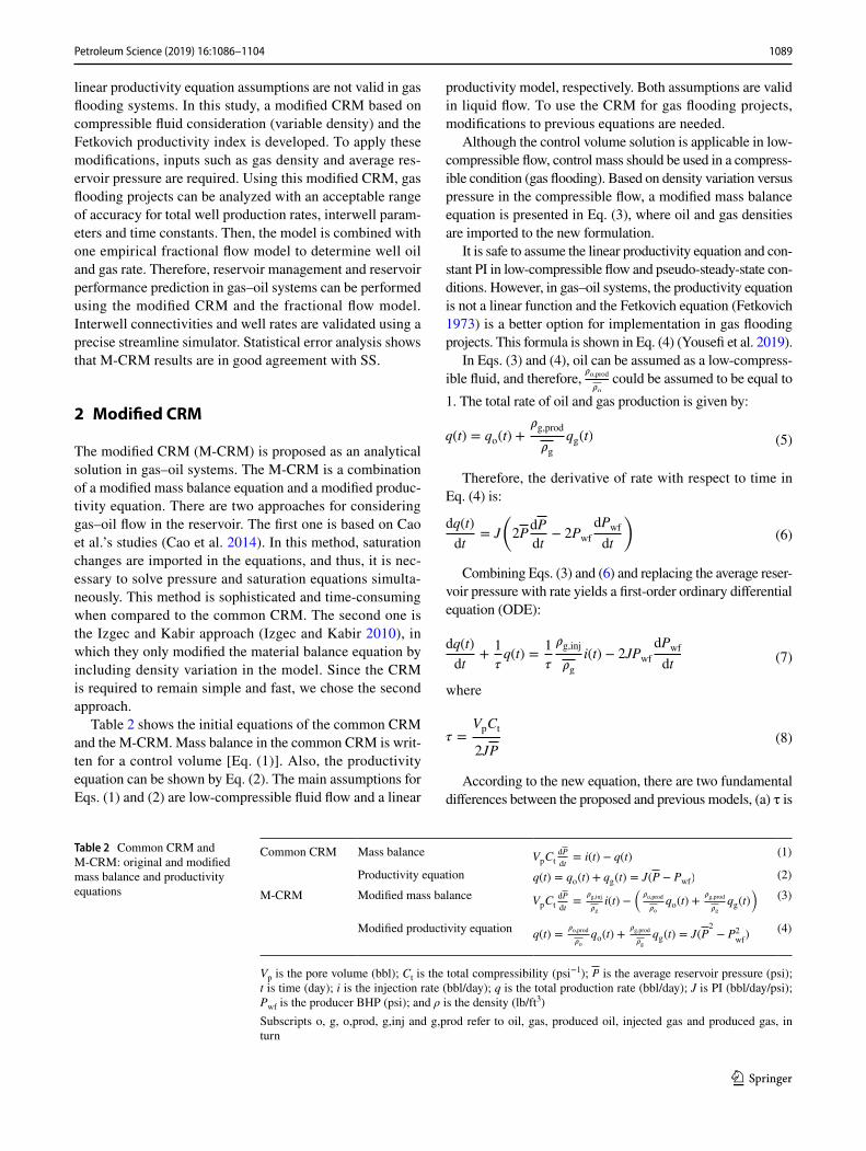
Table 2 shows the initial equations of the common CRM and the M-CRM. Mass balance in the common CRM is writ-ten for a control volume [Eq. (1)]. Also, the productivity equation can be shown by Eq. (2). The main assumptions for Eqs. (1) and (2) are low-compressible fluid flow and a linear

productivity model, respectively. Both assumptions are valid in liquid flow. To use the CRM for gas flooding projects, modifications to previous equations are needed.

Although the control volume solution is applicable in low-compressible flow, control mass should be used in a compress-ible condition (gas flooding). Based on density variation versus pressure in the compressible flow, a modified mass balance equation is presented in Eq. (3), where oil and gas densities are imported to the new formulation.

It is safe to assume the linear productivity equation and con-stant PI in low-compressible flow and pseudo-steady-state con-ditions. However, in gas–oil systems, the productivity equation is not a linear function and the Fetkovich equation (Fetkovich 1973) is a better option for implementation in gas flooding projects. This formula is shown in Eq. (4) (Yousefi et al. 2019).

In Eqs. (3) and (4), oil can be assumed as a low-compress-ible fluid, and therefore, �o,prod

�o could be assumed to be equal to

1. The total rate of oil and gas production is given by:

Therefore, the derivative of rate with respect to time in Eq. (4) is:

Combining Eqs. (3) and (6) and replacing the average reser-voir pressure with rate yields a first-order ordinary differential equation (ODE):

where

According to the new equation, there are two fundamental differences between the proposed and previous models, (a) τ is

(5)q(t) = qo(t) +�g,prod

�gqg(t)

(6)dq(t)

dt= J

(

2PdP

dt− 2Pwf

dPwf

dt

)

(7)dq(t)

dt+

1

�q(t) =

1

�

�g,inj

�gi(t) − 2JPwf

dPwf

dt

(8)� =VpCt

2JP

Table 2 Common CRM and M-CRM: original and modified mass balance and productivity equations

Vp is the pore volume (bbl); Ct is the total compressibility (psi−1); P is the average reservoir pressure (psi); t is time (day); i is the injection rate (bbl/day); q is the total production rate (bbl/day); J is PI (bbl/day/psi); Pwf is the producer BHP (psi); and ρ is the density (lb/ft3)Subscripts o, g, o,prod, g,inj and g,prod refer to oil, gas, produced oil, injected gas and produced gas, in turn

Common CRM Mass balance VpCtdP

dt= i(t) − q(t) (1)

Productivity equation q(t) = qo(t) + qg(t) = J(P − Pwf) (2)

M-CRM Modified mass balance VpCtdP

dt=

�g,inj

�gi(t) −

(�o,prod

�oqo(t) +

�g,prod

�gqg(t)

)(3)

Modified productivity equationq(t) =

�o,prod

�oqo(t) +

�g,prod

�gqg(t) = J(P

2− P2

wf)

(4)

1090 Petroleum Science (2019) 16:1086–1104

1 3

not constant and is a function of average reservoir pressure in each time step (with the unit of day/psi) and (b) density change affects injection rates and consequently, interwell parameters. Thus, the time constant and coefficient of interwell connectiv-ity are affected by the proposed modifications.

The analytical solution of Eq. (7) is as follows:

where q(t0) and � are the initial production rate (bbl/day) and the variable of integration, respectively.

Equation (9) presents a simple solution of M-CRM in the integral form. The right-hand side of this equation shows that the production rate which consists of three terms, namely primary depletion, gas injection effect and BHP changes. According to the equations developed by Sayarpour et al. (Sayarpour et al. 2007, 2009), three different control volumes were developed (Fig. 2). A constant injection rate during each time interval, constant PI and linear BHP drop for producers for the control volumes in the reservoir (the entire reservoir, the producer drainage and the injector–pro-ducer pair drainage) and the new formulations by superposi-tion in time are reported in Table 3. Moreover, the objective function for each method is determined.

(9)

q(t) = q(t0)e−(t−t0)

� + e−t

�

�=t

∫�=t0

1

�

�g,inj

�ge

�

� i(�)d� − e−t

�

�=t

∫�=t0

2e�

� JPwf

dPwf

d�d�

In CRM, fij is the interwell connectivity, which is math-ematically defined as:

where ninj, nprod and nt are the number of producers, injectors and time steps. Subscripts i, j, ij and k refer to injectors, producers, well pair (injector-producer) and time indices, respectively. Subscripts obs and cal represent observed and calculated data, respectively. Also, ΔPk

wf,j= Pk

wf,j− Pk−1

wf,j and

Δtk = tk − tk−1.

3 Workflow

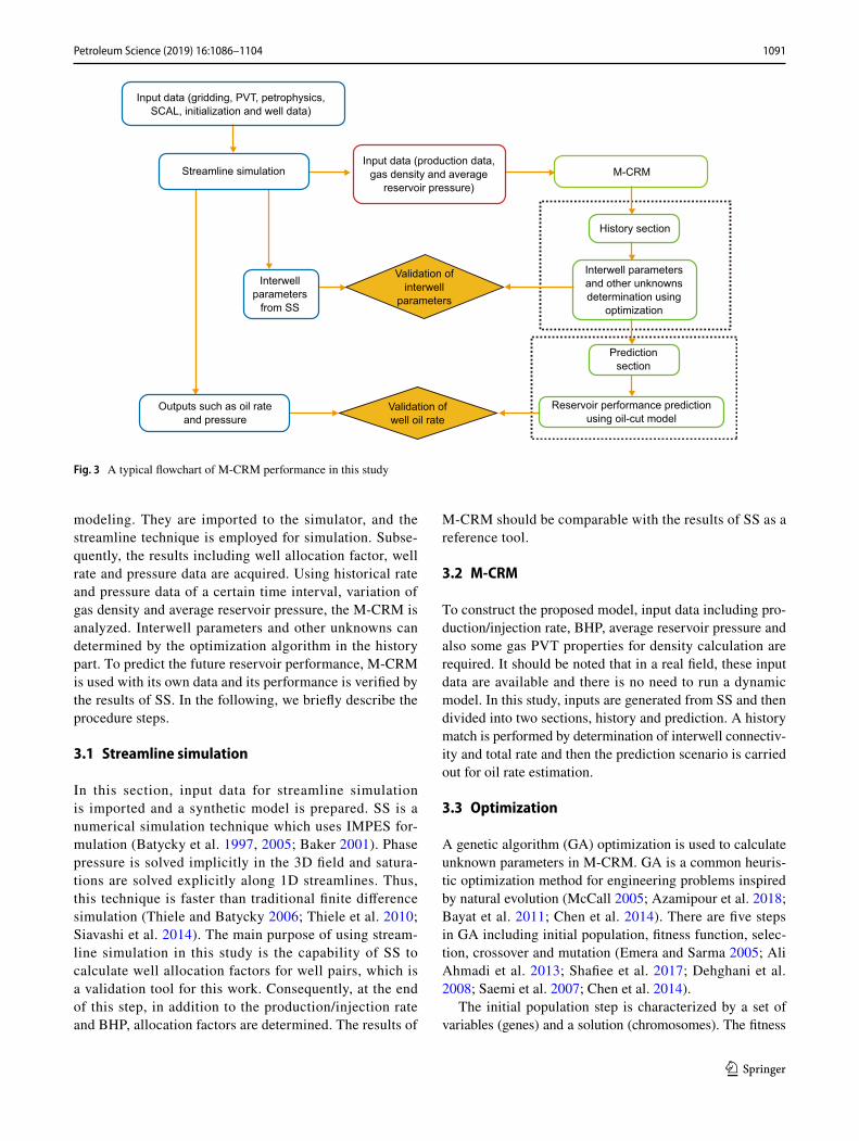
In the current study, a synthetic model is used. Rate and pressure data are generated from numerical simulation and then the M-CRM is used. Reliability of the proposed model in immiscible gas flooding conditions is investigated through the detailed procedure illustrated in Fig. 3. The following procedure is carried out to evaluate the M-CRM’s applica-bility in gas–oil systems.

Input data including gridding, SCAL, petrophysics, PVT, initialization and well data are required for dynamic

(13)fij =qij(t)

ii(t)fij ≥ 0,

Ninj∑

i=1

fij ≤ 1

iF(t) ii+1

qj(t) qj

ii

fijf′jii3

i2i1

ii

fij

f1j f2j

f3j

f11f12 f1Npre

fi+1jiNinj fNinj j

qF(t)

τFτj

τij

(a) (b) (c)

Fig. 2 a CRMT (capacitance–resistance model—tank based) with a single injector and producer in a control volume of a field. b CRMP (capaci-tance–resistance model—producer based) with one producer and surrounding injectors in a control volume of producer j. c CRMIP (capaci-tance–resistance model—injector/producer based) in a control volume between each injector/producer pair (Sayarpour 2008)

Table 3 Formulations of CRMs based on different control volumes and their objective functions

Method Equation No. of equation Objective function

CRMTq(tk) = q(tk−1)e

−Δtk

� +

(1 − e

−Δtk

�

)(

im�g,inj

�g− 2J�Pwf

ΔPkwf,j

Δt

)(10)

minz =nt∑

k=1

�qkobs

− qkcal

�2

CRMPqj(tk) = qj(tk−1)e

−Δtk

�j +

�

1 − e−Δtk

�j

��Ninj∑

i=1

�fij

�g,inj

�giki(t)�− 2Jj�jPwf

ΔPkwf,j

Δt

�(11)

minz =nt∑

k=1

nprod∑

j=1

�qkj,obs

− qkj,cal

�2

CRMIPqij(tk) = qij(tk−1)e

−Δtk

�ij +

(

1 − e

−Δtk�ij

)[

fij�g,inj

�giki− 2Jij�ijPwf ,j

ΔPkwf,j

Δtk

] (12)minz =

nt∑

k=1

nprod∑

j=1

�

qkj,obs

−

ninj∑

i=1

qkij,cal

�2

1091Petroleum Science (2019) 16:1086–1104

1 3

modeling. They are imported to the simulator, and the streamline technique is employed for simulation. Subse-quently, the results including well allocation factor, well rate and pressure data are acquired. Using historical rate and pressure data of a certain time interval, variation of gas density and average reservoir pressure, the M-CRM is analyzed. Interwell parameters and other unknowns can determined by the optimization algorithm in the history part. To predict the future reservoir performance, M-CRM is used with its own data and its performance is verified by the results of SS. In the following, we briefly describe the procedure steps.

3.1 Streamline simulation

In this section, input data for streamline simulation is imported and a synthetic model is prepared. SS is a numerical simulation technique which uses IMPES for-mulation (Batycky et al. 1997, 2005; Baker 2001). Phase pressure is solved implicitly in the 3D field and satura-tions are solved explicitly along 1D streamlines. Thus, this technique is faster than traditional finite difference simulation (Thiele and Batycky 2006; Thiele et al. 2010; Siavashi et al. 2014). The main purpose of using stream-line simulation in this study is the capability of SS to calculate well allocation factors for well pairs, which is a validation tool for this work. Consequently, at the end of this step, in addition to the production/injection rate and BHP, allocation factors are determined. The results of

M-CRM should be comparable with the results of SS as a reference tool.

3.2 M‑CRM

To construct the proposed model, input data including pro-duction/injection rate, BHP, average reservoir pressure and also some gas PVT properties for density calculation are required. It should be noted that in a real field, these input data are available and there is no need to run a dynamic model. In this study, inputs are generated from SS and then divided into two sections, history and prediction. A history match is performed by determination of interwell connectiv-ity and total rate and then the prediction scenario is carried out for oil rate estimation.

3.3 Optimization

A genetic algorithm (GA) optimization is used to calculate unknown parameters in M-CRM. GA is a common heuris-tic optimization method for engineering problems inspired by natural evolution (McCall 2005; Azamipour et al. 2018; Bayat et al. 2011; Chen et al. 2014). There are five steps in GA including initial population, fitness function, selec-tion, crossover and mutation (Emera and Sarma 2005; Ali Ahmadi et al. 2013; Shafiee et al. 2017; Dehghani et al. 2008; Saemi et al. 2007; Chen et al. 2014).

The initial population step is characterized by a set of variables (genes) and a solution (chromosomes). The fitness

Input data (gridding, PVT, petrophysics,SCAL, initialization and well data)

Input data (production data,gas density and average

reservoir pressure)

Interwell parametersand other unknownsdetermination using

optimization

Predictionsection

Validation ofwell oil rate

Validation ofinterwell

parameters

Interwellparameters

from SS

Outputs such as oil rateand pressure

Reservoir performance predictionusing oil-cut model

M-CRM

History section

Streamline simulation

Fig. 3 A typical flowchart of M-CRM performance in this study

1092 Petroleum Science (2019) 16:1086–1104

1 3

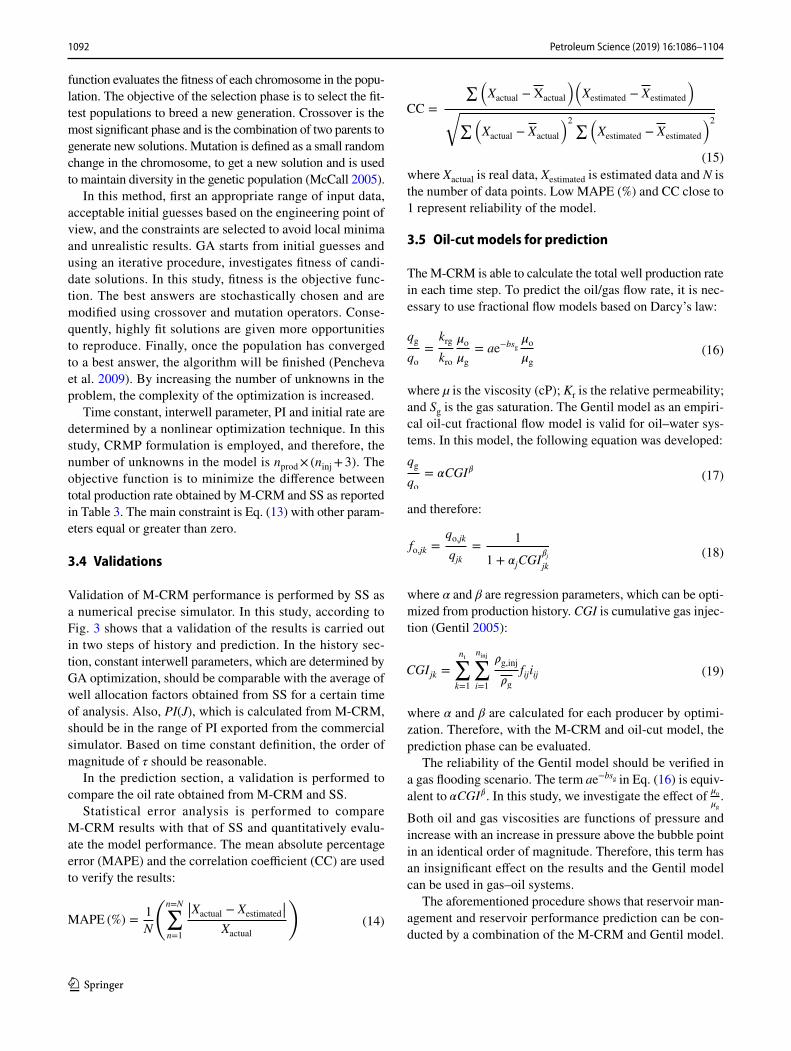
function evaluates the fitness of each chromosome in the popu-lation. The objective of the selection phase is to select the fit-test populations to breed a new generation. Crossover is the most significant phase and is the combination of two parents to generate new solutions. Mutation is defined as a small random change in the chromosome, to get a new solution and is used to maintain diversity in the genetic population (McCall 2005).

In this method, first an appropriate range of input data, acceptable initial guesses based on the engineering point of view, and the constraints are selected to avoid local minima and unrealistic results. GA starts from initial guesses and using an iterative procedure, investigates fitness of candi-date solutions. In this study, fitness is the objective func-tion. The best answers are stochastically chosen and are modified using crossover and mutation operators. Conse-quently, highly fit solutions are given more opportunities to reproduce. Finally, once the population has converged to a best answer, the algorithm will be finished (Pencheva et al. 2009). By increasing the number of unknowns in the problem, the complexity of the optimization is increased.

Time constant, interwell parameter, PI and initial rate are determined by a nonlinear optimization technique. In this study, CRMP formulation is employed, and therefore, the number of unknowns in the model is nprod × (ninj + 3). The objective function is to minimize the difference between total production rate obtained by M-CRM and SS as reported in Table 3. The main constraint is Eq. (13) with other param-eters equal or greater than zero.

3.4 Validations

Validation of M-CRM performance is performed by SS as a numerical precise simulator. In this study, according to Fig. 3 shows that a validation of the results is carried out in two steps of history and prediction. In the history sec-tion, constant interwell parameters, which are determined by GA optimization, should be comparable with the average of well allocation factors obtained from SS for a certain time of analysis. Also, PI(J), which is calculated from M-CRM, should be in the range of PI exported from the commercial simulator. Based on time constant definition, the order of magnitude of τ should be reasonable.

In the prediction section, a validation is performed to compare the oil rate obtained from M-CRM and SS.

Statistical error analysis is performed to compare M-CRM results with that of SS and quantitatively evalu-ate the model performance. The mean absolute percentage error (MAPE) and the correlation coefficient (CC) are used to verify the results:

(14)MAPE (%) =1

N

(n=N∑

n=1

||Xactual − Xestimated||

Xactual

)

where Xactual is real data, Xestimated is estimated data and N is the number of data points. Low MAPE (%) and CC close to 1 represent reliability of the model.

3.5 Oil‑cut models for prediction

The M-CRM is able to calculate the total well production rate in each time step. To predict the oil/gas flow rate, it is nec-essary to use fractional flow models based on Darcy’s law:

where µ is the viscosity (cP); Kr is the relative permeability; and Sg is the gas saturation. The Gentil model as an empiri-cal oil-cut fractional flow model is valid for oil–water sys-tems. In this model, the following equation was developed:

and therefore:

where α and β are regression parameters, which can be opti-mized from production history. CGI is cumulative gas injec-tion (Gentil 2005):

where α and β are calculated for each producer by optimi-zation. Therefore, with the M-CRM and oil-cut model, the prediction phase can be evaluated.

The reliability of the Gentil model should be verified in a gas flooding scenario. The term ae−bsg in Eq. (16) is equiv-alent to �CGI� . In this study, we investigate the effect of �o

�g

.

Both oil and gas viscosities are functions of pressure and increase with an increase in pressure above the bubble point in an identical order of magnitude. Therefore, this term has an insignificant effect on the results and the Gentil model can be used in gas–oil systems.

The aforementioned procedure shows that reservoir man-agement and reservoir performance prediction can be con-ducted by a combination of the M-CRM and Gentil model.

(15)

CC =

∑�Xactual − Xactual

��Xestimated − Xestimated

�

�∑�

Xactual − Xactual

�2 ∑�Xestimated − Xestimated

�2

(16)qg

qo=

krg

kro

�o

�g

= ae−bsg�o

�g

(17)qg

qo= �CGI�

(18)fo,jk =qo,jk

qjk=

1

1 + �jCGI�j

jk

(19)CGIjk =

nt∑

k=1

ninj∑

i=1

�g,inj

�gfijiij

1093Petroleum Science (2019) 16:1086–1104

1 3

The M-CRM cannot be substituted for commercial reservoir simulators but can be used as a reliable and robust method for simple and quick reservoir performance analysis.

4 Results and discussion

In this section, the proposed model is verified by a synthetic model. Interwell connectivity and oil rates are estimated based on the M-CRM, and the results are compared with SS. In order to evaluate the effect of reservoir parameters on accuracy of the model, sensitivity analysis for drawdown pressure and gas PVT properties is performed.

4.1 Description of the base case

PUNQ-S3 is a benchmark synthetic reservoir model which was extracted from a real field and is owned by the Elf Explo-ration and Production Company (Juanes et al. 2006; Gu and Oliver 2005). This reservoir is a popular test case for reservoir engineering problems. In this study, the reservoir structure (gridding and geometry) and geological properties are taken from PUNQ-S3. Figure 4 shows a 3D schematic of the model. Also, Fig. 5 demonstrates permeability and porosity maps of the reservoir. The initial reservoir condition is undersaturated with connate water. The model consists of 19 × 28 × 5 grid blocks at a depth of more than 7680 ft. We use this model to analyze the proposed M-CRM performance for an immiscible gas flooding project. Tables 4 and 5 show other reservoir and fluid parameters of the base case, where B is the formation volume factor and µ is the viscosity. Relative permeability curves for oil–water and gas–oil are depicted in Fig. 6.

There are 4 vertical oil producers and 2 vertical gas injec-tors in the model, and all wells are completed in 5 layers.

Production wells are controlled by random oil rates and are limited by minimum BHP, which is 3450 psi. Also, for gas injectors, the gas rate is a target and maximum BHP is the constraint. Production and injection BHPs are maintained above the bubble point pressure (3400.5 psi). Therefore, the source of produced gas is only from gas injectors. Also, the pressure is kept below minimum miscibility pressure to maintain an immiscible displacement.

The simulation is performed for 2520 days to verify the model by the M-CRM. Figure 7 displays the GOR of producers in the model. The new model can be applied in pre-breakthrough and post-breakthrough conditions with acceptable results (Yousefi et al. 2019). In this study, the post-breakthrough condition is chosen for interwell connec-tivity determination and also to predict oil production rates. Production life is divided into two sections (history and pre-diction). The history part is used to obtain unknown param-eters, and the prediction part is designed to evaluate the performance of the model in the next time steps. 1200 days are selected for the history match and the remaining time (510 days) is used for scenario prediction (Fig. 7). A com-parison between the M-CRM and common CRM perfor-mance was previously published in a paper by (Yousefi et al. 2019). They showed improvement of using the M-CRM in immiscible gas flooding over the common CRM. In this study, a thorough analysis of the M-CRM is performed in history and prediction parts using sensitivity analysis.

4.2 Analysis of the base case

There are 20 unknowns consisting of fij, τ, Jj and q0 in the model based on the M-CRM. The GA optimization is used for determination of the unknowns. Since there could be numerous solutions in optimization problems, the initial guesses of unknowns are very important. Therefore, the logical input data based on the constraints and nature of this engineering problem guarantees correct answers for unknowns. Table 6 presents optimization results for deter-mination of the unknowns in the PUNQ-S3 model. All parameters are acceptable values regarding the nature of the problem. Interwell parameters (fINJ1−j and fINJ12−j) should be comparable with the average of allocation factors obtained from the SS results.

Table 7 presents interwell connectivity parameters of M-CRM and SS in the history part. Also, the MAPE and CC of the total well production rate are reported in this table. Figure 8 shows the oil production from each well in the prediction part, which is calculated by the Gentil model. The MAPE and CC of the oil rate for all wells are 6.56% and 0.92, respectively. Results indicate the accuracy of the proposed model for interwell parameters calculated as well as the oil rate prediction (Fig. 8).

7686 7749 7813 7877 7940

PRO-4

PRO-11PRO-15

PRO-5

INJ-12

INJ-1

Depth, ft

Fig. 4 A 3D schematic and structural map (feet) of the PUNQ-S3 synthetic reservoir model

1094 Petroleum Science (2019) 16:1086–1104

1 3

(b)(a)

PRO-5 PRO-5

PRO-4 PRO-4

PRO-11

0.01 0.08 0.15

Porosity Permeability, mD

0.23 0.30 0.50 250.2 499.8 749.5 999.1

PRO-11

PRO-15 PRO-15

INJ-12 INJ-12

INJ-1 INJ-1

Fig. 5 a Porosity (fraction) and b permeability (mD) maps of the base case

Table 4 Reservoir parameters of the base case

Parameter Value

Model dimensions 19 × 28 × 5Number of cells 2660 (1757 active

cells)Datum depth, ft 7726.4Average porosity, % 13.94Average horizontal permeability, mD 269.9Average vertical permeability, mD 122.49Initial pressure@7726.4 ft, psi 3900.6Initial water saturation 0.12STOIIP (standard oil initially in-place),

MMSTB164.66

Rock compressibility, psi−1 2.1 × 10−6

Total pore volume at reservoir condition, MMbbl

223.76

Number of oil producers 4Number of gas injectors 2Drive mechanisms Rock compaction

and fluid expan-sion/gas injection

Table 5 Fluid properties of the base case

Parameter Value

Reference pressure Pref, psi 3400WaterBw, bbl/STB 1.01µw, cP 0.5Cw, psi−1 1.73 × 10−6

OilBo, bbl/STB 1.20µo, cP 1.46Pb, psi 3400.5Initial GOR (gas/oil ratio), scf/STB 415.5GasBg, bbl/Mscf 0.78µg, cP 0.013

1095Petroleum Science (2019) 16:1086–1104

1 3

4.3 Sensitivity analysis

According to Eqs.  (7) and (8), the proposed model was obtained by applying modifications regarding interwell connectivity and time constant in the common CRM. These modifications were related to the average reservoir pressure and gas properties. Therefore, to show the M-CRM’s capa-bility in all ranges of reservoir conditions, the drawdown

0

0.2

0.4

0.6

0.8

1.0

0 0.2 0.4 0.6 0.8 1.0

Rel

ativ

e pe

rmea

bilit

y

Water saturation

Krw

Krow

0 0.2 0.4 0.6 0.8 1.0

Rel

ativ

e pe

rmea

bilit

y

Gas saturation

Krg

Krog

0

0.2

0.4

0.6

0.8

1.0(a) (b)

Fig. 6 Relative permeability curves for a oil–water and b gas–oil of the base case

0

0.5

1.0

1.5

2.0

2.5

3.0

3.5

4.0

0 325 650 975 1300 1625 1950 2275 2600

Wel

l GO

R, M

scf/S

TB

Time, days

Well PRO-11 Well PRO-15 Well PRO-4 Well PRO-5

PredictionHistory

Post-breakthroughPre-breakthrough

Fig. 7 GOR of production wells in history and prediction parts

Table 6 Determination of unknown parameters in M-CRM by GA optimization

Producer �j × P , day fINJ1−j f

INJ12−j Jj q0j , bbl/d

PRO-4 415 0.280 0.249 18.98 68,408PRO-5 72 0.025 0.248 19.84 82,931PRO-11 282 0.441 0.000 4.24 16,427PRO-15 327 0.254 0.503 8.00 30,649

1096 Petroleum Science (2019) 16:1086–1104

1 3

pressure (DP) and gas PVT properties are investigated. Other parameters such as permeability, measurement noise,

number of measurements, total compressibility and number of producers were investigated by (Kaviani et al. 2014).

4.3.1 Drawdown pressure

Drawdown pressure is an important dynamic parameter in fluid flow through the reservoir especially for gas–oil sys-tems. To investigate its effect on the M-CRM performance, four cases are selected and the PUNQ-S3 model is simu-lated. All the parameters except the injection rate (the injec-tion pressure) are identical in the four cases. Oil and gas rate controls are chosen for producers and injectors, respectively, and the well BHP is the constraint with 16 unknown param-eters. The model performance is investigated for 2700 days. The length of history and prediction sections are 1800 and 900 days, respectively.

Four cases with different injection rates (injection pres-sure) are selected, and the average drawdown pressures for each case are calculated. Table 8 shows the effect of DP on

Table 7 Interwell parameters from SS and M-CRM

Well pair Interwell connectivity Total rate prediction, bbl/d

SS M-CRM MAPE, % CC

INJ-1PRO-4 0.277 0.280PRO-5 0.000 0.025PRO-11 0.470 0.441PRO-15 0.253 0.254 2.65 0.972INJ-12PRO-4 0.248 0.249PRO-5 0.249 0.248PRO-11 0.001 0.000PRO-15 0.503 0.503

200

400

600

800

0 110 220 330 440 550

Wel

l oil

rate

, bbl

/day

Time, days

M-CRM - PRO-4 SS - PRO-4

200

400

600

800

0 110 220 330 440 550

Wel

l oil

rate

, bbl

/day

Time, days

M-CRM - PRO-5 SS - PRO-5

200

400

600

800

0 110 220 330 440 550

Wel

l oil

rate

, bbl

/day

Time, days

M-CRM - PRO-11 SS - PRO-11

300

500

700

900

0 110 220 330 440 550

Wel

l oil

rate

, bbl

/day

Time, days

M-CRM - PRO-15 SS - PRO-15

CC = 0.90MAPE = 9.47%

CC = 0.96MAPE = 6.06%

CC = 0.93MAPE = 7.54%

CC = 0.90MAPE = 3.16%

(a) (b)

(c) (d)

Fig. 8 Well oil production rate in prediction part (510 days)

1097Petroleum Science (2019) 16:1086–1104

1 3

M-CRM performance in the history and prediction parts. The MAPE and CC for total oil production in the history section and for oil production in the prediction section are

also reported. Results show that estimated values are in good agreement with the real data.

The term �g,inj�g

which was added to the new model was

developed based on consideration of variations of gas prop-erties with pressure. Thus, this term compensates for the errors which are caused by the common CRM and is appli-cable in all pressure ranges (Yousefi et al. 2019). Figure 9 presents cross-plots of interwell parameters for the M-CRM and SS in the history section. Figure 10 shows error distribu-tion curves of the predicted oil rate using the Gentil model in the prediction section and relative error percent for pre-dicted rates of 4 producers (120 points). Results show that at all ranges of DP, the reliability of the model for interwell

Table 8 Effect of drawdown pressure on M-CRM performance

Case Average draw-down pressure, psi

History per-formance, total production

Prediction performance, oil production

MAPE, % CC MAPE, % CC

(1) Base case 157.2 4.24 0.92 6.41 0.85(2) 91.26 2.07 0.95 4.69 0.81(3) 275.04 4.48 0.95 7.25 0.90(4) 389.53 3.30 0.78 10.93 0.73

0

0.2

0.4

0.6

0.8

1.0

0 0.2 0.4 0.6 0.8 1.0

M-CRM interwell connectivity M-CRM interwell connectivity

M-CRM interwell connectivity M-CRM interwell connectivity

Drawdown pressure = 91.26 psi

(a) (b)

(c) (d)

0

0.2

0.4

0.6

0.8

1.0

0 0.2 0.4 0.6 0.8 1.0

Drawdown pressure = 157.2 psi

INJ-1INJ-12

0

0.2

0.4

0.6

0.8

1.0

0 0.2 0.4 0.6 0.8 1.0

Drawdown pressure = 275.04 psi

INJ-1INJ-12

0

0.2

0.4

0.6

0.8

1.0

0 0.2 0.4 0.6 0.8 1.0

SS

inte

rwel

l par

amet

ers

SS

inte

rwel

l par

amet

ers

SS

inte

rwel

l par

amet

ers

SS

inte

rwel

l par

amet

ers

INJ-1INJ-12

Drawdown pressure = 389.53 psi

INJ-1INJ-12

Fig. 9 Cross-plots of interwell parameters (M-CRM vs. SS) in the history section—effect of drawdown pressure

1098 Petroleum Science (2019) 16:1086–1104

1 3

connectivity determination and oil rate prediction is acceptable.

4.3.2 Gas properties

In this section, the effect of PVT properties of injected gas such as viscosity and formation volume factor (density) on the M-CRM performance is investigated. Since oil is a low-compressible fluid, the variation of its properties has negligible impact on the proposed model. In addition to the base case, a lower and a higher viscosity case and a lower and higher gas formation volume factor (FVF) are assumed

(Fig. 11). All properties except gas viscosity and FVF are identical for the five cases. Time intervals between 2220 and 5460 days (3270 days) are considered for model perfor-mance analysis, 2160 days for the history part and 1110 days for the prediction part.

Table 9 reports the effect of gas viscosity and FVF on the M-CRM performance in the history and prediction peri-ods in the PUNQ-S3 model. The MAPE in history and pre-diction sections are both below 5% and 10%, respectively, which show the strength of the M-CRM in a wide range of gas PVT properties. Also, CCs have quite an acceptable range (close to 1).

-40

-20

0

20

40R

elat

ive

erro

r, %

Data point

Drawdown pressure = 91.26 psi

MPE = −1.97%

-60

-40

-20

0

20

40

60

Rel

ativ

e er

ror,

%

Data point

Drawdown pressure = 157.2 psi

-40

-20

0

20

40

Rel

ativ

e er

ror,

%

Data point

Drawdown pressure = 275.04 psi

-60

-40

-20

0

20

40

60

Rel

ativ

e er

ror,

%

Data point

Drawdown pressure = 389.53 psi

MPE = −4.06%

MPE = −5.12%

MPE = −0.63%

(a) (b)

(c) (d)

Fig. 10 Error distribution curves of oil rate prediction from M-CRM in the prediction part—effect of drawdown pressure

1099Petroleum Science (2019) 16:1086–1104

1 3

Figure 12 displays cross-plots of interwell parameters in the history section for different gas properties. Results show that the proposed model correctly predicts interwell parameters in various operational conditions. Addition-ally, gas viscosity and FVF do not have negative effects on the results. The error distribution curves of estimated oil rate in the prediction section are demonstrated in Fig. 13. Although the Gentil model tends to underpre-dict the oil rate in many data points, generally the results are acceptable and reflect suitable performance of the M-CRM.

It is noted that more reliable results for the total rate in the history period and the oil rate in the prediction period are obtained when high gas viscosity and low gas FVF are incorporated for the injected gas. This behavior is a result of gas deviation from the ideal behavior in low viscosity and high FVF conditions. Thus, in these conditions, the M-CRM performance leads to high errors.

5 Conclusions

This study presented a new formulation for CRM (M-CRM) as a simple tool for reservoir performance analysis and pre-diction in immiscible gas flooding projects. New modifi-cations using gas density variation and average reservoir pressure affected interwell connectivity parameters and time constants in the proposed model. A combination of the M-CRM and the Gentil model was employed for a compre-hensive analysis of the PUNQ-S3 synthetic model in history and prediction sections. From the results of this study, we concluded that:

• A detailed flowchart for M-CRM performance evaluation in history-matching and future reservoir performance prediction in immiscible gas flooding was introduced. Furthermore, we used streamline simulation for valida-tion of the results and a genetic algorithm for optimizing unknown parameters.

• The M-CRM was performed on a synthetic reservoir model under immiscible gas flooding. The total pro-duction rates of wells and interwell parameters in the history part and oil production rates in the prediction part were estimated with an acceptable relative error (below 10%) and a correlation coefficient (close to 1).

• By considering a variable gas density with pressure, the high drawdown pressure did not have a negative impact on the validity of the M-CRM and Gentil model.

• Gas PVT properties such as viscosity and FVF did not affect the M-CRM robustness in the immiscible gas flooding process. Although employing low gas viscos-

0

0.005

0.010

0.015

0.020

0.025

0.030

0 1000 2000 3000

Gas

vis

cosi

ty, c

P

Pressure, psi

Lower viscosityBase caseHigher viscosity

0

2

4

6

8

10

12

0 1000 2000 3000

Gas

FV

F, b

bl/M

scf

Pressure, psi

Lower FVFBase caseHigher FVF

(a) (b)

Fig. 11 Base case, higher and lower cases for a viscosity and b gas FVF

Table 9 Effect of gas PVT properties on the M-CRM performance

Case History performance, total production

Prediction perfor-mance, oil produc-tion

MAPE, % CC MAPE, % CC

(1) Base case 3.14 0.95 8.73 0.91(2) Higher viscosity 2.76 0.96 7.20 0.94(3) Lower viscosity 4.09 0.91 9.07 0.89(4) Higher FVF 4.66 0.94 8.36 0.93(5) Lower FVF 3.38 0.93 5.38 0.96

1100 Petroleum Science (2019) 16:1086–1104

1 3

INJ-1

INJ-12

0

0.2

0.4

0.6

0.8

1.0

0 0.2 0.4 0.6 0.8 1.0

SS

inte

rwel

l par

amet

ers

M-CRM interwell connectivity

Lower FVF (5)

(e)

0

0.2

0.4

0.6

0.8

1.0

0 0.2 0.4 0.6 0.8 1.0

M-CRM interwell connectivity M-CRM interwell connectivity

M-CRM interwell connectivityM-CRM interwell connectivity

Base case (1)

INJ-1

INJ-12

INJ-1

INJ-12

INJ-1

INJ-12

INJ-1

INJ-12

0

0.2

0.4

0.6

0.8

1.0

0 0.2 0.4 0.6 0.8 1.0

Higher viscosity (2)

0

0.2

0.4

0.6

0.8

1.0

0 0.2 0.4 0.6 0.8 1.0

Lower viscosity (3)

0

0.2

0.4

0.6

0.8

1.0

0 0.2 0.4 0.6 0.8 1.0

SS

inte

rwel

l par

amet

ers

SS

inte

rwel

l par

amet

ers

SS

inte

rwel

l par

amet

ers

SS

inte

rwel

l par

amet

ers

Higher FVF (4)

(a) (b)

(c) (d)

Fig. 12 Cross-plots of interwell parameters (M-CRM vs. SS) in the history section—effect of gas properties

1101Petroleum Science (2019) 16:1086–1104

1 3

-60

-40

-20

0

20

40

60(a) (b)

(c)

(e)

(d)

Rel

ativ

e er

ror,

%

Data point

Base case (1)

-60

-40

-20

0

20

40

60

Rel

ativ

e er

ror,

%

Data point

Higher viscosity (2)

-80

-60

-40

-20

0

20

40

60

80

Rel

ativ

e er

ror,

%

Data point

Lower viscosity (3)

-80

-60

-40

-20

0

20

40

60

80

Rel

ativ

e er

ror,

%

Data point

Higher FVF (4)

-60

-40

-20

0

20

40

60

Rel

ativ

e er

ror,

%

Data point

Lower FVF (5)

MPE= -2.22%

MPE= -6.23% MPE= -3.85%

MPE= -4.79%MPE= -6.19%

Fig. 13 Error distribution curves of oil rate prediction form the M-CRM in the prediction part—effect of gas properties

1102 Petroleum Science (2019) 16:1086–1104

1 3

ity and high gas FVF resulted in relatively high errors, the M-CRM performance is acceptable.

Open Access This article is distributed under the terms of the Crea-tive Commons Attribution 4.0 International License (http://creat iveco mmons .org/licen ses/by/4.0/), which permits unrestricted use, distribu-tion, and reproduction in any medium, provided you give appropriate credit to the original author(s) and the source, provide a link to the Creative Commons license, and indicate if changes were made.

References

Agrawal P, Kumar J, Draoui E. Lesson learnt from immiscible gas injection pilot in offshore carbonate reservoir. In: Abu Dhabi international petroleum exhibition & conference. Society of Petroleum Engineers; 2016. https ://doi.org/10.2118/18339 4-MS.

Al-Khamis MN, Ozkan E, Raghavan RS. Analysis of interference tests with horizontal wells. SPE Reserv Eval Eng. 2005;8(04):337–47. https ://doi.org/10.2118/84292 -PA.

Ali Ahmadi M, Zendehboudi S, Lohi A, Elkamel A, Chatzis I. Res-ervoir permeability prediction by neural networks combined with hybrid genetic algorithm and particle swarm optimization. Geophys Prospect. 2013;61(3):582–98. https ://doi.org/10.1111/j.1365-2478.2012.01080 .x.

Alkhazmi B, Sohrabi M, Farzaneh SA. An experimental investigation of the effect of gas and water slug size and injection order on the performance of immiscible WAG injection in a mixed-wet system. In: SPE Kuwait oil & gas show and conference. Society of Petroleum Engineers; 2017. https ://doi.org/10.2118/18753 7-MS.

Artun E. Characterizing interwell connectivity in waterflooded reser-voirs using data-driven and reduced-physics models: a compara-tive study. J Neural Comput Appl. 2017;28(7):1729–43. https ://doi.org/10.1007/s0052 1-015-2152-0.

Azamipour V, Assareh M, Mittermeir GM. An improved optimiza-tion procedure for production and injection scheduling using a hybrid genetic algorithm. Chem Eng Res Des. 2018;131:557–70. https ://doi.org/10.1016/j.cherd .2017.11.022.

Azin R, Nasiri A, Entezari J. Underground gas storage in a partially depleted gas reservoir. Oil Gas Sci Technol Revue de l’IFP. 2008;63(6):691–703. https ://doi.org/10.2516/ogst:20080 28.

Baker R. Streamline technology: reservoir history matching and fore-casting: its success, limitations, and future. J Can Pet Technol. 2001. https ://doi.org/10.2118/01-04-DAS.

Batycky R, Blunt MJ, Thiele MR. A 3D field-scale streamline-based reservoir simulator. SPE Reserv Eng. 1997;12(04):246–54. https ://doi.org/10.2118/36726 -PA.

Batycky RP, Thiele MR, Baker RO, Chung S. Revisiting reservoir flood-surveillance methods using streamlines. In: SPE annual technical conference and exhibition. Society of Petroleum Engi-neers; 2005. https ://doi.org/10.2118/95402 -MS.

Bayat M, Rahimpour M, Moghtaderi B. Genetic algorithm strategy (GA) for optimization of a novel dual-stage slurry bubble column membrane configuration for Fischer–Tropsch synthesis in gas to liquid (GTL) technology. J Nat Gas Sci Eng. 2011;3(4):555–70. https ://doi.org/10.1016/j.jngse .2011.06.004.

Bybee K. Improved gas storage: deliverability enhancements and new storage facilities. J Pet Technol. 2001;53(04):68–70. https ://doi.org/10.2118/0401-0068-JPT.

Cao F, Luo H, Lake LW. Development of a fully coupled two-phase flow based capacitance resistance model (CRM). In: SPE improved oil recovery symposium. Society of Petroleum Engi-neers; 2014. https ://doi.org/10.2118/16948 5-MS.

Chen G, Fu K, Liang Z, Sema T, Li C, Tontiwachwuthikul P, et al. The genetic algorithm based back propagation neural network for MMP prediction in CO2-EOR process. Fuel. 2014;126:202–12. https ://doi.org/10.1016/j.fuel.2014.02.034.

de Holanda RW, Gildin E, Jensen JL. A generalized framework for capacitance resistance models and a comparison with streamline allocation factors. J Pet Sci Eng. 2018;162:260–82. https ://doi.org/10.1016/j.petro l.2017.10.020.

Dehghani SM, Sefti MV, Ameri A, Kaveh NS. Minimum miscibility pressure prediction based on a hybrid neural genetic algorithm. Chem Eng Res Des. 2008;86(2):173–85. https ://doi.org/10.1016/j.cherd .2007.10.011.

Delshad M, Bastami A, Pourafshary P. The use of capacitance–resis-tive model for estimation of fracture distribution in the hydro-carbon reservoir. In: SPE Saudi Arabia section technical sym-posium. Society of Petroleum Engineers; 2009. https ://doi.org/10.2118/12607 6-MS.

Demiryurek U, Banaei-Kashani F, Shahabi C, Wilkinson FG. Neural-network based sensitivity analysis for injector-producer rela-tionship identification. In: Intelligent energy conference and exhibition. Society of Petroleum Engineers; 2008. https ://doi.org/10.2118/11212 4-MS.

Dinges DD, Ogbe DO. A method for analyzing pulse tests con-sidering wellbore storage and skin effects. SPE Form Eval. 1988;3(04):743–50. https ://doi.org/10.2118/15582 -PA.

Dinh AV, Tiab D. Interpretation of interwell connectivity tests in a waterflood system. In: SPE annual technical conference and exhibition. Society of Petroleum Engineersl; 2008. https ://doi.org/10.2118/11614 4-MS.

Du Y, Guan L. Interwell tracer tests: lessons learned from past field studies. In: SPE Asia Pacific oil and gas conference and exhi-bition. Society of Petroleum Engineers; 2005. https ://doi.org/10.2118/93140 -MS.

Dugstad Ø, Aurdal T, Galdiga C, Hundere I, Torgersen H. Application of tracers to monitor fluid flow in the Snorre field: a field study. In: SPE annual technical conference and exhibition. Society of Petroleum Engineers; 1999. https ://doi.org/10.2118/56427 -MS.

Emera MK, Sarma HK. Use of genetic algorithm to estimate CO2–oil minimum miscibility pressure—a key parameter in design of CO2 miscible flood. J Pet Sci Eng. 2005;46(1–2):37–52. https ://doi.org/10.1016/j.petro l.2004.10.001.

Eshraghi SE, Rasaei MR, Zendehboudi S. Optimization of miscible CO2 EOR and storage using heuristic methods combined with capacitance/resistance and Gentil fractional flow models. J Nat Gas Sci Eng. 2016;32:304–18. https ://doi.org/10.1016/j.jngse .2016.04.012.

Fedenczuk L, Hoffmann K. Surveying and analyzing injection responses for patterns with horizontal wells. In: SPE interna-tional conference on horizontal well technology; 1998. https ://doi.org/10.2118/50430 -MS.

Fetkovich M. The isochronal testing of oil wells. In: Fall meeting of the society of petroleum engineers of AIME. Society of Petroleum Engineers; 1973. https ://doi.org/10.2118/4529-MS.

Fokker PA, Borello ES, Serazio C, Verga F. Estimating reservoir het-erogeneities from pulse testing. J Pet Sci Eng. 2012;86:15–26. https ://doi.org/10.1016/j.petro l.2012.03.017.

Gentil PH. The use of multilinear regression models in patterned water-floods: physical meaning of the regression coefficients. Master’s thesis, The University of Texas at Austin. 2005.

Gherabati SA, Hughes RG, White CD, Zhang H. A large scale network model to obtain interwell formation characteristics. Int J Oil Gas Coal Technol. 2017a;15(1):1–24. https ://doi.org/10.1504/IJOGC T.2017.08385 6.

Gherabati SA, Takbiri-Borujeni A, Hughes R. Heterogeneity quanti-fication in waterfloods using a multiphase network approach. J

1103Petroleum Science (2019) 16:1086–1104

1 3

Nat Gas Sci Eng. 2017b;40:299–311. https ://doi.org/10.1016/j.jngse .2017.02.023.

Gu Y, Oliver DS. History matching of the PUNQ-S3 reservoir model using the ensemble Kalman filter. SPE J. 2005;10(02):217–24. https ://doi.org/10.2118/89942 -PA.

Heffer KJ, Fox RJ, McGill CA, Koutsabeloulis NC. Novel techniques show links between reservoir flow directionality, earth stress, fault structure and geomechanical changes in mature waterfloods. SPE J. 1997;2(02):91–8. https ://doi.org/10.2118/30711 -PA.

Huang X, Ling Y. Water injection optimization using historical pro-duction and seismic data. In: SPE annual technical conference and exhibition. Society of Petroleum Engineers; 2006. https ://doi.org/10.2118/10249 9-MS.

Huseby OK, Andersen M, Svorstol I, Dugstad O. Improved understand-ing of reservoir fluid dynamics in the North Sea Snorre field by combining tracers, 4D seismic, and production data. SPE Reserv Eval Eng. 2008;11(04):768–77. https ://doi.org/10.2118/10528 8-PA.

Izgec O, Kabir C. Understanding reservoir connectivity in waterfloods before breakthrough. J Pet Sci Eng. 2010;75(1):1–12. https ://doi.org/10.1016/j.petro l.2010.10.004.

Jansen F, Kelkar M. Application of wavelets to production data in describing inter-well relationships. In: SPE annual technical con-ference and exhibition. Society of Petroleum Engineers; 1997. https ://doi.org/10.2118/38876 -MS.

Juanes R, Spiteri E, Orr F, Blunt M. Impact of relative permeabil-ity hysteresis on geological CO2 storage. Water Resour Res. 2006;42(12):5–9. https ://doi.org/10.1029/2005W R0048 06.

Kaviani D, Jensen JL, Lake LW. Estimation of interwell connectivity in the case of unmeasured fluctuating bottomhole pressures. J Pet Sci Eng. 2012;90:79–95. https ://doi.org/10.1016/j.petro l.2012.04.008.

Kaviani D, Soroush M, Jensen JL. How accurate are Capacitance Model connectivity estimates? J Pet Sci Eng. 2014;122:439–52. https ://doi.org/10.1016/j.petro l.2014.08.003.

Kaviani D, Valkó PP. Inferring interwell connectivity using multiwell productivity index (MPI). J Pet Sci Eng. 2010;73(1):48–58. https ://doi.org/10.1016/j.petro l.2010.05.006.

Kostelnik K, Arredondo P, Montenegro A. A case history on Califor-nia immiscible gas injection, Elk Hills Field. In: SPE western regional meeting. Society of Petroleum Engineers; 2017. https ://doi.org/10.2118/18565 5-MS.

Koval E. A method for predicting the performance of unstable mis-cible displacement in heterogeneous media. Soc Pet Eng J. 1963;3(02):145–54. https ://doi.org/10.2118/450-PA.

Kulkarni MM, Rao DN. Experimental investigation of miscible and immiscible Water-Alternating-Gas (WAG) process performance. J Pet Sci Eng. 2005;48(1–2):1–20. https ://doi.org/10.1016/j.petro l.2005.05.001.

Kumar J, Agrawal P, Draoui E. A case study on miscible and immisci-ble gas-injection pilots in a Middle East carbonate reservoir in an offshore environment. SPE Reserv Eval Eng. 2017;20(01):19–29. https ://doi.org/10.2118/18175 8-PA.

Laochamroonvorapongse R, Kabir C, Lake LW. Performance assess-ment of miscible and immiscible water-alternating gas floods with simple tools. J Pet Sci Eng. 2014;122:18–30. https ://doi.org/10.1016/j.petro l.2014.08.012.

Lichtenberger G. Field applications of interwell tracers for reservoir characterization of enhanced oil recovery pilot areas. In: SPE pro-duction operations symposium. Society of Petroleum Engineers; 1991. https ://doi.org/10.2118/21652 -MS.

Liu F, Mendel JM, Nejad AM. Forecasting injector/producer relationships from production and injection rates using an extended Kalman filter. SPE J. 2009;14(04):653–64. https ://doi.org/10.2118/11052 0-PA.

Mamghaderi A, Pourafshary P. Water flooding performance prediction in layered reservoirs using improved capacitance–resistive model.

J Pet Sci Eng. 2013;108:107–17. https ://doi.org/10.1016/j.petro l.2013.06.006.

McCall J. Genetic algorithms for modelling and optimisation. J Com-put Appl Math. 2005;184(1):205–22. https ://doi.org/10.1016/j.cam.2004.07.034.

Miri R, Zendehboudi S, Kord S, Vargas F, Lohi A, Elkamel A, et al. Experimental and numerical modeling study of gravity drain-age considering asphaltene deposition. Ind Eng Chem Res. 2014;53(28):11512–26. https ://doi.org/10.1021/ie404 424p.

Mirzayev M, Jensen JL. Measuring interwell communication using the capacitance model in tight reservoirs. In: SPE western regional meeting. Society of Petroleum Engineers; 2016. https ://doi.org/10.2118/18042 9-MS.

Mohammadi S, Kharrat R, Khalili M, Mehranfar M. Optimal conditions for immiscible recycle gas injection process: a simulation study for one of the Iranian oil reservoirs. Sci Iran. 2011;18(6):1407–14. https ://doi.org/10.1016/j.scien t.2011.10.003.

Moreno GA. Multilayer capacitance–resistance model with dynamic connectivities. J Pet Sci Eng. 2013;109:298–307. https ://doi.org/10.1016/j.petro l.2013.08.009.

Moreno GA, Lake LW. Input signal design to estimate interwell connectivities in mature fields from the capacitance–resistance model. Pet Sci. 2014a;11(4):563–8. https ://doi.org/10.1007/s1218 2-014-0372-z.

Moreno GA, Lake LW. On the uncertainty of interwell connectiv-ity estimations from the capacitance–resistance model. Pet Sci. 2014b;11(2):265–71. https ://doi.org/10.1007/s1218 2-014-0339-0.

Ogbe D, Brigham W. A correlation for interference testing with well-bore-storage and skin effects. SPE Form Eval. 1989;4(03):391–6. https ://doi.org/10.2118/13253 -pa.

Panda M, Chopra A. An integrated approach to estimate well interac-tions. In: SPE India oil and gas conference and exhibition. Society of Petroleum Engineers; 1998. https ://doi.org/10.2118/39563 -MS.

Pencheva T, Atanassov K, Shannon A. Modelling of a roulette wheel selection operator in genetic algorithms using generalized nets. Int J Bioautom. 2009;13(4):257–64.

Rafiei Y. Improved oil production and waterflood performance by water allocation management. PhD. Dissertation. Heriot-Watt Univer-sity; 2014.

Refunjol BT, Lake LW. Memoir 71, Chapter 15: reservoir characteriza-tion based on tracer response and rank analysis of production and injection rates; 1999.

Rezaei N, Zendehboudi S, Chatzis I, Lohi A. Combined benefits of capillary barrier and injection pressure control to improve fluid recovery at breakthrough upon gas injection: an experimen-tal study. Fuel. 2018;211:638–48. https ://doi.org/10.1016/j.fuel.2017.09.048.

Saemi M, Ahmadi M, Varjani AY. Design of neural networks using genetic algorithm for the permeability estimation of the reservoir. J Pet Sci Eng. 2007;59(1–2):97–105. https ://doi.org/10.1016/j.petro l.2007.03.007.

Salazar-Bustamante M, Gonzalez-Gomez H, Matringe SF, Castineira D. Combining decline-curve analysis and capacitance/resist-ance models to understand and predict the behavior of a mature naturally fractured carbonate reservoir under gas injection. In: SPE Latin America and Caribbean petroleum engineering con-ference. Society of Petroleum Engineers; 2012. https ://doi.org/10.2118/15325 2-MS.

Sayarpour M. Development and application of capacitance–resistive models to water/carbon dioxide floods. The University of Texas at Austin; 2008.

Sayarpour M, Zuluaga E, Kabir CS, Lake LW. The use of capacitance–resistive models for rapid estimation of waterflood performance. In: SPE annual technical conference and exhibition. Society of Petroleum Engineers; 2007. https ://doi.org/10.2118/11008 1-MS.

1104 Petroleum Science (2019) 16:1086–1104

1 3

Sayarpour M, Zuluaga E, Kabir CS, Lake LW. The use of capacitance–resistance models for rapid estimation of waterflood performance and optimization. J Pet Sci Eng. 2009;69(3):227–38. https ://doi.org/10.1016/j.petro l.2009.09.006.

Shafiee A, Nomvar M, Liu Z, Abbas A. A new genetic algorithm based on prenatal genetic screening (PGS-GA) and its applica-tion in an automated process flowsheet synthesis problem for a membrane based carbon capture case-study. Chem Eng Res Des. 2017;128:265–89. https ://doi.org/10.1016/j.cherd .2017.10.009.

Siavashi M, Blunt MJ, Raisee M, Pourafshary P. Three-dimensional streamline-based simulation of non-isothermal two-phase flow in heterogeneous porous media. Comput Fluids. 2014;103:116–31. https ://doi.org/10.1016/j.compfl uid.2014.07.014.

Soroush M, Kaviani D, Jensen JL. Interwell connectivity evaluation in cases of changing skin and frequent production interruptions. J Pet Sci Eng. 2014;122:616–30. https ://doi.org/10.1016/j.petro l.2014.09.001.

Stewart G, Gupta A. The interpretation of interference tests in a reser-voir with sealing and partially communicating faults. In: European petroleum conference. Society of Petroleum Engineers; 1984. https ://doi.org/10.2118/12967 -MS.

Tao Q, Bryant SL. Optimizing carbon sequestration with the capaci-tance/resistance model. SPE J. 2015;20(5):1094–120. https ://doi.org/10.2118/17407 6-PA.

Thiele MR, Batycky R, Fenwick D. Streamline simulation for modern reservoir-engineering workflows. J Pet Technol. 2010;62(01):64–70. https ://doi.org/10.2118/11860 8-JPT.

Thiele MR, Batycky RP. Using streamline-derived injection efficien-cies for improved waterflood management. SPE Reserv Eval Eng. 2006;9(02):187–96. https ://doi.org/10.2118/84080 -PA.

Valko PP, Doublet L, Blasingame T. Development and application of the multiwell productivity index (MPI). SPE J. 2000;5(01):21–31. https ://doi.org/10.2118/51793 -PA.

Weber D, Edgar TF, Lake LW, Lasdon LS, Kawas S, Sayarpour M. Improvements in capacitance–resistive modeling and opti-mization of large scale reservoirs. In: SPE western regional

meeting. Society of Petroleum Engineers; 2009. https ://doi.org/10.2118/12129 9-MS.

Yin Z, Ayzenberg M, MacBeth C, Feng T, Chassagne R. Enhance-ment of dynamic reservoir interpretation by correlating mul-tiple 4D seismic monitors to well behavior. Interpretation. 2015;3(2):SP35–52. https ://doi.org/10.1190/INT-2014-0194.1.

Yin Z, MacBeth C, Chassagne R, Vazquez O. Evaluation of inter-well connectivity using well fluctuations and 4D seismic data. J Pet Sci Eng. 2016;145:533–47. https ://doi.org/10.1016/j.petro l.2016.06.021.

Yousef AA, Gentil PH, Jensen JL, Lake LW. A capacitance model to infer interwell connectivity from production and injec-tion rate fluctuations. In: SPE annual technical conference and exhibition. Society of Petroleum Engineers; 2005. https ://doi.org/10.2118/95322 -MS.

Yousef AA, Jensen JL, Lake LW. Integrated interpretation of inter-well connectivity using injection and production fluctuations. Math Geosci. 2009;41(1):81–102. https ://doi.org/10.1007/s1100 4-008-9189-x.

Yousef AA, Lake LW, Jensen JL. Analysis and interpretation of inter-well connectivity from production and injection rate fluctuations using a capacitance model. In: SPE/DOE symposium on improved oil recovery. Society of Petroleum Engineers; 2006. https ://doi.org/10.2118/99998 -MS.

Yousefi SH, Rashidi F, Sharifi M, Soroush M. On determination of interwell connectivity under immiscible gas injection process: modified capacitance–resistance model. Can J Chem Eng. 2019;97(4):1008–21. https ://doi.org/10.1002/cjce.23294 .

Yuncong G, Mifu Z, Jianbo W, Chang Z. Performance and gas break-through during CO2 immiscible flooding in ultra-low perme-ability reservoirs. Pet Explor Dev. 2014;41(1):88–95. https ://doi.org/10.1016/S1876 -3804(14)60010 -0.

Zhang Z, Li H, Zhang D. Reservoir characterization and production optimization using the ensemble-based optimization method and multi-layer capacitance–resistive models. J Pet Sci Eng. 2017;156:633–53. https ://doi.org/10.1016/j.petro l.2017.06.020.