Embed Size (px)
Citation preview
Prediction of ignition limits with respect to fuel fraction of inert gases.
Evaluation of cost effective CFD-method using cold flow simulations Johan Sjölander EN1524 Master thesis, 30 ECTS, for a Degree of Master of Science in Energy Engineering Department of Applied Physics and Electronics Umeå University, 2015
i
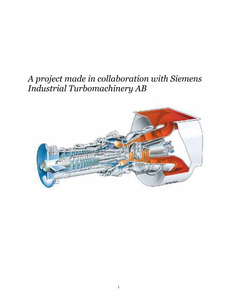
A project made in collaboration with Siemens Industrial Turbomachinery AB

ii
Abstract Improving fuel flexibility for gas turbines is one advantageous property on the market. It may
lead to increased feasibility by potential customers and thereby give increased competiveness
for production and retail companies of gas turbines such as Siemens Industrial Turbomachinery
in Finspång. For this reason among others SIT assigned Anton Berg to perform several ignition
tests at SIT’s atmospheric combustion rig (ACR) as his master thesis project. In the ACR he
tested the limits for how high amounts of inert gases (N2 and CO2) that the rig, prepared with the
3rd generation DLE-burner operative in both the SGT-700 and SGT-800 engine, could ignite on
(Berg, 2012).
Research made by Abdel-Gay and Bradley already in 1985 summarized methane and propane
combustion articles showing that a Karlovitz number ( ⁄ ) of
1.5 could be used as a quenching limit for turbulent combustion (Abdel-Gayed & Bradley, 1985).
Furthermore in 2010 Shy et al. showed that the Karlovitz number showed good correlation to
ignition transition from a flamelet to distributed regime (Shy, et al., 2010). They also showed that
this ignition transition affected the ignition probability significantly.
Based on the results of these studies among others a CFD concept predicting ignition
probability from cold flow simulations were created and tested in several applications at
Cambridge University (Soworka, et al., 2014) (Neophytou, et al., 2012). With Berg’s ignition
tests as reference results and a draft for a cost effective ignition prediction model this thesis
where started.
With the objectives of evaluating the ignition prediction against Berg’s results and at the same
time analyze if there would be any better suited igniter spot 15 cold flow simulations on the ACR
burner and combustor geometry were conducted. Boundary conditions according to selected
tests were chosen with fuels composition ranging from pure methane/propane to fractions of
40/60 mole% CO2 and 50/75 mole% N2.
By evaluating the average Karlovitz number in spherical ignition volumes around the igniter
position successful ignition could be predicted if the Karlovitz number were below 1.5. The
results showed promising tendencies but no straightforward prediction could be concluded from
the evaluated approach. A conclusion regarding that the turbulence model probably didn’t
predict mixing good enough was made which implied that no improved igniter position could be
recommended. However by development of the approach by using a more accurate turbulence
model as LES for example may improve the mixing and confirm the good prediction tendencies
found. Possibilities for significantly improved ignition limits were also showed for 3-19% increase
in equivalence ratio around the vicinity of the igniter.
iii
Table of Contents Abstract....................................................................................................................................... ii
Acknowledgements ..................................................................................................................... v
Nomenclature ............................................................................................................................ vi
1 Introduction ............................................................................................................................. 1
1.1 Siemens ........................................................................................................................... 1
1.2 Siemens Industrial Turbomachinery .................................................................................. 2
1.3 Fuel flexibility .................................................................................................................... 3
1.4 The Atmospheric Combustion Rig at SIT .......................................................................... 4
1.4.1 Ignition tests in the ACR ............................................................................................. 5
1.4.3 The DLE-burner and some of its characteristics ......................................................... 8
1.5 Why Computational Fluid Dynamics (CFD) ......................................................................10
1.6 Objectives ........................................................................................................................11
1.7 Boundaries ......................................................................................................................11
2 Fluid Mechanics .....................................................................................................................12
2.1 Conservation of mass ......................................................................................................12
2.2 Conservation of momentum .............................................................................................15
2.3 Closure of the equations – The Navier-Stokes equations ................................................18
2.4 Conservation of energy ....................................................................................................19
2.5 Turbulence ......................................................................................................................21
2.5.1 Vortex stretching and the Kolmogorov’s hypothesis ..................................................22
2.6 Reynolds Averaged Navier-Stokes Equations .................................................................23
2.6.1 Turbulence models and closure of the RANS equations ............................................24
3 Flame Theory .........................................................................................................................26
3.1 Combustion regimes ........................................................................................................27
3.2 Ignition Theory .................................................................................................................29
3.3 MIE – Minimum Ignition Energy .......................................................................................30
4 Methodology .......................................................................................................................35
4.1 Grid generation ................................................................................................................36
4.1.1 Mesh quality ..............................................................................................................37
4.2 Pre processing.................................................................................................................38
4.3 Post processing ...............................................................................................................39
4.4 Chemical simulations in GENE-AC ..................................................................................39

iv
4.4.1 Laminar flame speed and flame thickness.................................................................39
4.5 Ignition evaluation ............................................................................................................41
5 Results of pre-studies ............................................................................................................43
5.1 GENE-AC results and validation ......................................................................................43
5.2 Grid study ........................................................................................................................52
5.3 Comparison to Ansys Fluent ............................................................................................60
5.4 Sensitivity analysis ..........................................................................................................63
6 Evaluation of ignition model ...................................................................................................67
6.1 CFD influence on ignition prediction ................................................................................70
7 Evaluation of alternative ignition spots ...................................................................................82
7.1 Methane/CO2 ...................................................................................................................83
8 Discussion .............................................................................................................................85
8.1 Conclusions .....................................................................................................................87
9 Recommendations for future work ..........................................................................................88
Bibliography ..............................................................................................................................90
Appendix ...................................................................................................................................93

v
Acknowledgements This thesis of 30 ECTS was performed as the last part of the Master of Science in Energy
Engineering education program at Umeå University.
Through long project like this you always hit obstacles on the way. At those moments however
there’s usually invaluable support and guidance from different people around you, thereby I
would like to thank the following people:
First of all I would like to thank the combustion group, with Anders Häggmark as its manager, at
Siemens Industrial Turbomachinery for providing me the honor of doing my master thesis at
their division.
Special thanks go to my supervisors Anton Berg and Dr. Daniel Lörstad for their irreplaceable
guidance and feedback throughout my project.
Dr. Darioush Gohari Barhaghi for help with settings and simulations for GENE-AC.
Lector Ronny Östin for help with improving the presentation and disposition of the report.
My master thesis colleague Dejan Korén for results from Ansys Fluent to compare with. Also
thank you for tips and tricks using the Ansys CFX software package and great resident
company.
My two fantastic friends Karolina Saveska and Adrian Pauli that has contributed to a higher
desire towards the workdays than the weekend.
My parents Gunilla and Jan Sjölander for staying positive and trying to put me in the right
direction mentally when work felt tough.
Finally I would like to thank my older sister Jannike Sjölander that seems to clean and adjust
your perspective whenever and whatever makes you feel like you have the world on your
shoulder.
Johan Sjölander
Finspång, Augusti 2015

vi
Nomenclature
⁄
⁄
⁄
-
-
⁄
⁄
-
m
⁄
-
⁄
⁄
-
⁄
⁄
⁄
⁄
⁄
⁄
vii
-
-
-
⁄
⁄
⁄
-
-
-
-
-
-
-
-
-
-
-
-
-
-
-
-
-
-
-
-
-

1
1 Introduction
1.1 Siemens Siemens was founded 1847 by Werner von Siemens and Johann Georg Halske under the name
“Telegraph Construction Company of Siemens & Halske”. The main production was then, as the
name imposes, the pointer telegraph developed by the founders. During the, soon to be, 170
yearlong development from past to presence Siemens has established in over 190 countries
and employ approximately 370 000 persons in total. (Siemens AB, Corporate Communications,
2013)
Moreover the original telegraph objective has developed into a handful of business sectors:
Healthcare, Energy, Industry and Infrastructure and cities.
Among Siemens large number of employees around 5000 of them work in divisions located in
Sweden. Siemens Industrial Turbomachinery (SIT) has its residence in Finspång and produces
gas turbines in the range of 19 to 50 MW power output. The business involves everything from
development and production to service which in total engage almost 3000 employees. (Siemens
Industrial Turbomachinery AB, 2013)

2
1.2 Siemens Industrial Turbomachinery Since the decision of moving the steam turbine production from Finspång to Görlitz, Germany, was made in 2011 (Sveriges televisions nyheter, 2011) the focus on SIT has solely been at gas turbines. The interval of 19 to 50 MW is spanned by 5 gas turbine engines named SGT-500, SGT-600, SGT-700, SGT-750 and SGT-800. Areas of operation can be everything from marine applications and power generation to mechanical drive for transport in oil pipelines. (Siemens Industrial Turbomachinery AB, 2013) Table 1. Short description of the gas turbines produced at SIT AB (Siemens Industrial Turbomachinery AB, 2013).
Model Efficiency Electrical power output
Properties
SGT-500 33.7% 19 MWe High power-to-weight ratio, high fuel flexibility (heavy oils and other residues from refinery processes), NOx emissions ≤ 42 ppmV. May be used for power generation and mechanical drive.
SGT-600 33.6% 24.5 MWe Flexible for gaseous fuel can handle high hydrogen contents, low NOx emissions ≤ 25ppmV. May be used for power generation and mechanical drive.
SGT-700 37.2% 33 MWe Good fuel flexibility and runs on gases with up to 50 vol-% N2 respectively 40 vol-% CO2. May be used for power generation and mechanical drive.
SGT-750 39.5% 37 MWe Introduced in Siemens gas turbine catalog in 2010 with the aim of great reliability and long service intervals, NOx emissions ≤ 15ppmV. May be used for power generation and mechanical drive.
SGT-800 38.3% 50.5 MWe Has the best emission performance in the 50-60 MWe class on dual fuel in the 50-100% load range. NOx emissions ≤ 15ppmV for gas fuels and ≤ 25ppmV for liquid fuels. Similar fuel flexibility as the SGT-700, they use the same burner. Mainly used for power generation, best in class for combined cycle efficiency >55%.
3
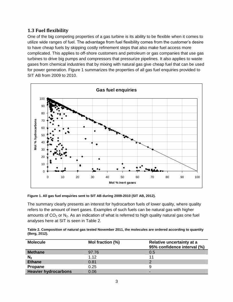
1.3 Fuel flexibility One of the big competing properties of a gas turbine is its ability to be flexible when it comes to
utilize wide ranges of fuel. The advantage from fuel flexibility comes from the customer’s desire
to have cheap fuels by skipping costly refinement steps that also make fuel access more
complicated. This applies to off-shore customers and petroleum or gas companies that use gas
turbines to drive big pumps and compressors that pressurize pipelines. It also applies to waste
gases from chemical industries that by mixing with natural gas give cheap fuel that can be used
for power generation. Figure 1 summarizes the properties of all gas fuel enquiries provided to
SIT AB from 2009 to 2010.
Figure 1. All gas fuel enquiries sent to SIT AB during 2009-2010 (SIT AB, 2012).
The summary clearly presents an interest for hydrocarbon fuels of lower quality, where quality
refers to the amount of inert gases. Examples of such fuels can be natural gas with higher
amounts of CO2 or N2. As an indication of what is referred to high quality natural gas one fuel
analyses here at SIT is seen in Table 2.
Table 2. Composition of natural gas tested November 2011, the molecules are ordered according to quantity (Berg, 2012).
Molecule Mol fraction (%) Relative uncertainty at a 95% confidence interval (%)
Methane 97.76 0.5 N2 1.12 11 Ethane 0.81 2 Propane 0.25 9 Heavier hydrocarbons 0.06 -
Gas fuel enquiries
0
10
20
30
40
50
60
70
80
90
100
0 10 20 30 40 50 60 70 80 90 100
Mol % inert gases
Mo
l %
hyd
rocarb
on
s
4
Among the five gas turbine models produced at SIT AB in Finspång the SGT-800 is the only
single-shaft engine while the SGT-500 is a triple-shaft engine and the rest are twin-shaft
engines. Twin-shaft turbines means that they’re divided into a shaft connecting the compressor
and the pressure turbine and one shaft connecting the power turbine to the work consuming
target. Twin-shaft engines are better suited for applications where regulation of the output rpm is
important. The SGT-700, which 3rd generation Dry Low Emission (DLE) burner in this case is
the target of study, has proven to run on low quality fuels at least from the perspective of
content. Hellberg and Nordén proved in 2009 that a standard SGT-700 had stable performance
on low, medium and full load even when fuel N2 increased to as much as 40 vol% (Hellberg &
Nordén, 2009).
When looking from the perspective of ignition (the start-up of the gas turbine) propane or natural
gas of high quality are standard fuels for the SGT-700. This becomes an undesired feature for
customers that run their engines on low quality gaseous fuels due to both the additional cost it
implies but also for reasons when it comes to handling propane. Since propane, in distinction to
methane, is of higher density than air leakages compose a risk both by means of explosions
and intoxication.
The current approach at SIT AB when uninvestigated fuel enquiries appear is simply to test the
ignition performance on a gas turbine which compared to a cost efficient analytical method is
both consuming more time and money.
1.4 The Atmospheric Combustion Rig at SIT The ACR located at SIT in Finspång is used for different combustion studies where atmospheric
conditions is reasonable to the application and thus gives cheaper and easier performed tests
compared to pressurized combustion.
One example of an application of the ACR is a study published by Lantz et al. where they used
the atmospheric rig together with measurements methods as OH PLIF and chemiluminescence
imaging. By this setup they investigated how natural gas got affected by hydrogen enrichment in
the sense of pressure drop, flame size, position and shape. (Lantz, et al., 2015)
Figure 2 on the next page shows a cross section of the ACR where the main components and
inlets are highlighted.

5
Figure 2. Schematic picture of the atmospheric combustion rig at SIT (Lantz, et al., 2015).
1.4.1 Ignition tests in the ACR
From the possibilities when it comes to development of ignition fuel flexibility Siemens gave the
assignment of a master thesis project to Anton Berg, then student at KTH, where he performed
and summarized several ignition tests on SIT’s atmospheric combustion rig (Berg, 2012).
The illustrated igniter in Figure 2 is the torch igniter and not the spark plug that was used for the
gas tests. Other modifications relative Figure 2 during the tests was that the emission probe
were replaced by a window to gain extra possibilities for visual analysis. The lower and lateral
optical access was used for video recording and optical insight respectively. Since ignition of a
gas turbine occurs at atmospheric pressure the ACR rig at SIT is in some sense ideal for the
tests made by Berg. It is also a cost effective set-up for parameter studies since a real SGT-700
consists of 18 DLE-burners, which would make the procedure more complicated and much
more staff would need to be involved. However this kind of small scale tests could never replace
the full scale tests that usually follow, they serve as a valuable guideline when deciding the full
scale test matrix and other subsequent analysis.
Berg made 84 ignition tests on gaseous fuels where every test consisted of a new fuel
composition (Berg, 2012). 13 of the tests were based on propane and the other 71 on natural
gas while CO2 and N2 were altered among the tests performed on the same fuel basis. For
natural gas a range from 0-35 mole% CO2 and 0-50 mole% N2 were studied and for propane
ranges of 0-50 mole% CO2 and 0-70 mole% N2 were studied. A standard mass flow of 170 g/s
was set for the air but for some cases of the methane ignitions the air flow was altered in 4
steps between the standard mass flow up to 220 g/s. The air had a temperature of 293 K and
the fuel temperature was assumed the same even though slight differences of fuel temperature
may have occurred due to expansion of the gas coming from the fuel tank. Different settings of
fuel flow for pure methane was evaluated and then set to the lowest flow where ignition was
stable. When the amount of inert gases was increased in the fuel composition the fuel flow was

6
increased to the amount that would give the same energy flow as the reference case, i.e. the
resulting adiabatic flame temperature after ignition was reduced with inert content.
When it comes to the spark igniter, Vibro-Meter S24328, used in the ACR and also the SGT-700
the ignition energy it delivers is not variable. This means that the Minimum Ignition Energy,
which is the lowest amount of energy needed to ignite a combustible mixture, was not possible
to be extracted from the test rig and therefore was calculated theoretically.
The definition of successful ignition determined was that each fuel composition needed to stand
three consecutive attempts of ignition where a propagating flame followed the initialization and
rapid growth of a flame kernel. For further details of the spark induced ignition sequence the
reader is referred to section 3.2.
Figure 3 presents a small part of the results gathered during this master thesis project. The
results show that on mole% basis propane ignites on higher amounts of inert gases. The results
also show that increased amount of CO2 increases the MIE more than the same amount of N2.
The ignition limits marked in Figure 3 is the practical result that serves as comparison to the
simulation results in this report.
Figure 3. Outcome from Anton’s master thesis where the MIE increase as a function of mole% inert gases is presented. Ignition limits for each fuel combination is inserted (Berg, 2012).
Anton examined relevant papers for MIE of gaseous fuels and made both a thorough review
and a summary of physical parameters that has been proven to affect the MIE. Table 3 on the
next page is a reconstruction of the table with the addition of the sources giving the statements
embedded directly in the table. Only the parameters suitable for the objectives of this thesis are
presented, for more information the reader is referred to (Berg, 2012) or the initial sources.
Figure 1. MIE limits as a function of molar-% (Berg, 2012)

7
Table 3. Parameters affecting the MIE for gaseous fuels (Berg, 2012).
Parameter Effect Degree of MIE impact
Optimum
Air flow Increased MIE for increased air flow.
Major (Ballal & Lefebvre, 1975)
Lowest possible
Turbulence intensity
Increased MIE for increased turbulence intensity.
Significant (Ballal & Lefebvre, 1977) Major for turbulent intensities above critical value (Shy, et al., 2010)
Lowest possible
Turbulence scale Increased MIE for increased turbulent scales under large turbulent intensities.
Significant (Ballal & Lefebvre, 1977)
Lowest possible
Fuel/air temperature
Decreased MIE for increased temperatures.
Severe (Brokaw & Gerstein , 1957)
Highest possible
Pressure Decreased MIE for increased pressures, dependent on air flow and equivalence ratio.
Major (Ballal & Lefebvre, 1975)
Highest possible
Fuel Decreased MIE for propane.
Insignificant (Ballal & Lefebvre, 1977)
Propane
Equivalence ratio Decreased MIE when moving away from near stoichiometric conditions.
Severe (Ballal & Lefebvre, 1975)
Slightly rich
Inert gases Increased MIE for increased amount inert gases.
5-10 times higher for methane (Ballal & Lefebvre, 1977)
As low as possible, CO2 has higher impact than N2
Spark plug location
- Severe (Marchione, et al., 2009)
Recirculation zone

8
1.4.3 The DLE-burner and some of its characteristics
The DLE-burner illustrated in Figure 2 can be seen in more detail in Figure 4. In the picture the
flow of the burner goes from right to left.
Figure 4. Main components of the 3rd generation DLE-burner applied in the ACR and the SGT-800 (SIT AB, 2012). The difference towards its application in the SGT-700 is that there’s no combustor hood.
What’s important to know is the fact that during ignition the pilot nozzle is the only fuel system that is active. This implies that the fuel doesn’t premix in the swirl cone and thus the igniting mixture will be fuel and air that is just partially premixed. The disarticulation that is made among different flames is if the combustible mixture is premixed or not and if the flow is of laminar or turbulent feature. The properties of each distinction are summarized in

9
Table 4.
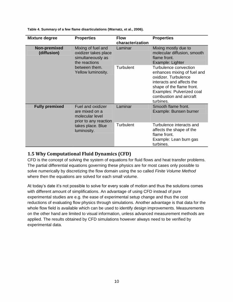
10
Table 4. Summary of a few flame disarticulations (Warnatz, et al., 2006).
Mixture degree Properties Flow characterization
Properties
Non-premixed (diffusion)
Mixing of fuel and oxidizer takes place simultaneously as the reactions between them. Yellow luminosity.
Laminar Mixing mostly due to molecular diffusion, smooth flame front. Example: Lighter
Turbulent Turbulence convection enhances mixing of fuel and oxidizer. Turbulence interacts and affects the shape of the flame front. Examples: Pulverized coal combustion and aircraft turbines.
Fully premixed Fuel and oxidizer are mixed on a molecular level prior to any reaction takes place. Blue luminosity.
Laminar Smooth flame front. Example: Bunsen burner
Turbulent Turbulence interacts and affects the shape of the flame front. Example: Lean burn gas turbines.
1.5 Why Computational Fluid Dynamics (CFD) CFD is the concept of solving the system of equations for fluid flows and heat transfer problems.
The partial differential equations governing these physics are for most cases only possible to
solve numerically by discretizing the flow domain using the so called Finite Volume Method
where then the equations are solved for each small volume.
At today’s date it’s not possible to solve for every scale of motion and thus the solutions comes
with different amount of simplifications. An advantage of using CFD instead of pure
experimental studies are e.g. the ease of experimental setup change and thus the cost
reductions of evaluating flow physics through simulations. Another advantage is that data for the
whole flow field is available which can be used to identify design improvements. Measurements
on the other hand are limited to visual information, unless advanced measurement methods are
applied. The results obtained by CFD simulations however always need to be verified by
experimental data.
11
1.6 Objectives From the competitive advantages from flexible fuel when it comes to ignition together with the
possibilities of cost reduction for analyze and development work when it comes to CFD the
following thesis was initialized. The objectives stated are:
• Evaluate cost effective prediction methodologies for ignition limits applicable to gas
turbine conditions, especially using the critical Karlovitz number according to the
strategies from (Soworka, et al., 2014).
• Apply these prediction methodologies to the SGT-700 burner in SIT’s ACR.
• Identify model which links and suggest model improvements for future work.
• Validate the methodology and estimate prediction accuracy by comparison to measured
data (Berg, 2012).
• Evaluate if igniter location in SIT ACR may be improved.
• Suggest how the ignition limits for a real gas turbine combustor geometry could be
investigated.
1.7 Boundaries Since this project, as most projects, is limited by time and resource limits the approach has to
be bounded by several conditions.
• RANS - Decreases computational power required
and thus time.
• Only simulation of gaseous fuels. - Multiphase flows is more complicated and
first of all gaseous fuel is of interest.
• Natural gas treated as methane. - For simplicity.
• Air simulated as containing 21% - For simplicity.
• Chemical kinetic models of - No models available for flames of non-
premixed flames used even premixed character.
though semi-premixed start-up.
12
2 Fluid Mechanics CFD is the abbreviation for Computational Fluid Dynamics and is a powerful computational tool
to numerically solve the equations governing fluid flows and other associated physics e.g. heat
transfer. Application areas of CFD include weather forecasting, drag reduction of cars and
combustion. The governing equations of fluid flows are the Navier-Stokes equations that are
derived from the conservation laws of mass, momentum and energy.
2.1 Conservation of mass The conservation of mass equation builds on the principle that mass can’t be created nor
destroyed, that is the mass of a closed system must remain constant. For fluid dynamics
applications this translates to that the net mass flow rate of a given control volume must equal
the time rate change of mass in that volume. This property can be described by
∫
∑
∑
(1)
The mass flow rate through one surface of the control volume expressed with a differential
approach is proportional to the area by the relation
(2)
Now assume the control volume is an infinitesimal box-shaped fluid element in Cartesian
coordinates where its dimension in the x, y and z direction is dx, dy and dz. Then let the fluid
density and the velocity components in all three directions be defined as respectively in
the center of the fluid element. Then the flux of mass at the center of the fluid element can be
expressed as the density times the velocity component in each direction respectively. By
performing a Taylor expansion the mass flux through each face of the control volume can be
obtained. Terms higher than first order can be neglected since their influence almost diminish
when the size of the control volume shrinks to sufficiently small proportions. If the coordinate
system is defined as Figure 5,

13
Figure 5. General three dimensional coordinate system
the Taylor expansion at the center of the right face equals
*
+
(3)
The principle of Taylor expansion is identical in all three dimensions so the remaining faces of
the control are practically obtained by exchanging the velocity and size to the right dimension
component. By combining equation 2 and 3 the net mass flow rate can be illustrated as Figure
6.

14
Figure 6. Net mass flow rate through a control volume
If the approach from Figure 6 is applied to the right hand side of equation 1 the flow into and out
of the control volume can be expressed as equation 4 and 5 respectively
∑
(
) (
) (
)
(4)
∑
(
) (
) (
)
(5)
For sufficiently small control volumes the integration operator of left hand side of equation 1 can
be discarded and replaced by multiplication of the density time derivative and the size of the
control volume in each direction
∫
(6)
By combining equation 4, 5 and 6 into equation 1 the conservation of mass can be described by
(𝜌𝑢 𝜕 𝜌𝑢
𝜕𝑥
𝑑𝑥
)𝑑𝑦𝑑𝑧 (𝜌𝑢
𝜕 𝜌𝑢
𝜕𝑥
𝑑𝑥
)𝑑𝑦𝑑𝑧
(𝜌𝑤 𝜕 𝜌𝑤
𝜕𝑧
𝑑𝑧
)𝑑𝑥𝑑𝑦
(𝜌𝑣 𝜕 𝜌𝑣
𝜕𝑦
𝑑𝑦
)𝑑𝑥𝑑𝑧
(𝜌𝑤 𝜕 𝜌𝑤
𝜕𝑧
𝑑𝑧
)𝑑𝑥𝑑𝑦
(𝜌𝑣 𝜕 𝜌𝑣
𝜕𝑦
𝑑𝑦
)𝑑𝑥𝑑𝑧
15
(
) (
) (
)
(
) (
)
(
)
(7)
This can be refined to what is referred to as the continuity equation
(8)
After division by and rearranging equation 8 becomes
( ) (9)
And for flows that can be regarded as incompressible it further reduces to
(10)
2.2 Conservation of momentum The conservation of momentum has its base in Newton’s second law of motion that is for a rigid
body of mass m
(11)
The last equality in equation 11 says that the net force on a body is equal to the time rate of
change of momentum on that body. When the net force acting on a body equals zero the
momentum is constant and thus conserved. To derive the conservation of momentum equation
one needs to specify whether the Eulerian or Lagrangian frame of reference is to be used. The
Lagrangian approach follows an individual fluid particle moving through space and time while
the Eulerian approach analysis the fluid flow on fixed locations in space. Using the former
approach the position in space of a particle can be defined by . Newton’s
second law applied to the particle then gives
(12)
Using the Lagrangian frame of reference a particles properties e.g. the velocity is equal to the
velocity field at its position at any given time-point. Using the chain rule together with the fact

16
that a particles position can be replaced by the corresponding position in Eulerian
coordinates then yields
( )
( )
(13)
( )
in the last equality above is referred to as the material derivative (Wendt, 2009).
The forces acting on a fluid element can be divided into body and surface forces. Body forces
act on the whole fluid element and the main body force in most cases is the gravity. The surface
forces are usually split into pressure forces and viscous stresses where the latter can be further
divided into shear and normal stresses (Wendt, 2009).
The pressure forces, the normal stress and the shear stress of each direction and fluid element
surface can be obtained by the same Taylor series expansion as was used for the conservation
of mass derivation (Wendt, 2009). Figure 7 summarize the surface forces in the x-direction
where the first index notation states which surface the stress acts on and the second index
notation states in which direction it acts.

17
Figure 7. Surface forces acting on a fluid element in the x-direction.
Summation of all the surface forces in the x-direction then yields that
∑ (
)
(14)
The general body force is the gravity, so the body force acting in the x-direction can be written
as
∑
(15)
By combining equations 13, 14 and 15 into equation 12 and divide it with the
conservation of momentum can be re-written as
(
)
(16)
(
)
By the same analogy the conservation of momentum in the y- and z-direction
(
) (
) (17)
(𝜏𝑧𝑥 𝜕𝜏𝑧𝑥𝜕𝑧
𝑑𝑧
)𝑑𝑥𝑑𝑦
(𝜏𝑧𝑥 𝜕𝜏𝑧𝑥𝜕𝑧
𝑑𝑧
)𝑑𝑥𝑑𝑦
(𝜏𝑦𝑥 𝜕𝜏𝑦𝑥
𝜕𝑦
𝑑𝑦
)𝑑𝑥𝑑𝑧
𝜏𝑥𝑥
𝜕𝜏𝑥𝑥𝜕𝑥
𝑑𝑥
(𝑝 𝜕𝑝
𝜕𝑥
𝑑𝑥
)
𝑑𝑦𝑑𝑧 (𝜏𝑦𝑥
𝜕𝜏𝑦𝑥
𝜕𝑦
𝑑𝑦
)𝑑𝑥𝑑𝑧
𝜏𝑥𝑥
𝜕𝜏𝑥𝑥𝜕𝑥
𝑑𝑥
(𝑝 𝜕𝑝
𝜕𝑥
𝑑𝑥
)
𝑑𝑦𝑑𝑧

18
(
) (
)
(18)
By implying the Einstein summation convention the general equation for the conservation of
momentum becomes
(
) (
)
(19)
Where the Einstein summation approach says
∑
(20)
2.3 Closure of the equations – The Navier-Stokes equations Counting all the variables of the conservation of mass and momentum equations in all three
dimensions you get 11 unknowns with only 4 equations to solve for these, the system of
equations is not closed. The trick is then to use the concept of Newtonian fluids that derives the
viscous stresses as a function of the viscosity and the shear strain rate. For Newtonian fluids
( )
{
(
) (
)
(
)
(
)
(
) (
)
}
(21)
The viscous stress term in equation 19 then becomes
( )
(22)
Since partial derivatives is independent of the order of derivation
(23)
And according to the continuity equation for incompressible flow
(24)
19
This compresses the incompressible form of the Navier-Stokes equations to
{
(
)
(25)
(26)
At today’s date there’s no possibility to generate general analytic solutions to these equations.
This is because of the term
that makes the equations a set of nonlinear PDE’s and no one
has succeed to find a solution for a general case of such equations (McMurtry, 2000).
2.4 Conservation of energy When solving adiabatic fluid dynamics for incompressible flows e.g. liquids equation 25 and 26
is closed for solving the pressure and velocity field in all three directions. In the case of
combustion or gas velocities above Mach numbers of 0.3 for example the fluid flow is in practice
compressible and thereby the conservation of energy needs to be introduced together with the
compressible N-S equations. The conservation of energy equation starts from the first law of
thermodynamics, energy can be transformed from one type to another but it can neither be
created nor destroyed.
The energy content of a closed system, e.g. a fluid element, is decided by heat transfer and
work transfer (Wendt, 2009). The first thermodynamic law written above can thus be described
according to
(27)
The net rate of work done on a fluid element is equal to the force times the velocity parallel with
the direction of the force, giving the rate of work due to body forces according to (Wendt, 2009)
( ) (28)
Again Figure 7 is used to sum all the surface forces in the x-direction. These are then multiplied
with the velocity to get the rate of work due to surface forces according to
*(
) (
)+
*(
) (
)+
(29)
*(
( )
) (
)+
20
[(
) (
)]
The big parentheses represents rate of work due to pressure forces, normal stresses and shear
stresses of the surfaces in the y and z coordinate direction respectively. If equation 29 is refined
and generalized for the forces in each direction the total work done on a fluid element can be
expressed as
( )
(30)
The net rate heat transfer of a fluid element can be divided into heat driven by temperature
gradients across its surfaces and volumetric heating such as combustion or radiation (Wendt,
2009). If the volumetric heat per unit mass is denoted as then the total volumetric heating of
a fluid element is
(31)
By letting , and be the heat transferred by thermal conduction through each face of the
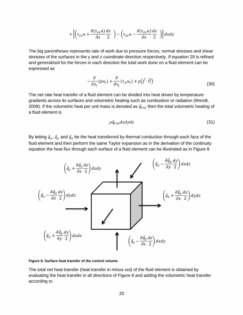
fluid element and then perform the same Taylor expansion as in the derivation of the continuity
equation the heat flux through each surface of a fluid element can be illustrated as in Figure 8
Figure 8. Surface heat transfer of the control volume
The total net heat transfer (heat transfer in minus out) of the fluid element is obtained by
evaluating the heat transfer in all directions of Figure 8 and adding the volumetric heat transfer
according to
(𝑞 𝑥 𝜕𝑞 𝑥𝜕𝑥
𝑑𝑥
)𝑑𝑦𝑑𝑧 (𝑞 𝑥
𝜕𝑞 𝑥𝜕𝑥
𝑑𝑥
)𝑑𝑦𝑑𝑧
(𝑞 𝑧 𝜕𝑞 𝑧𝜕𝑧
𝑑𝑧
)𝑑𝑥𝑑𝑦
(𝑞 𝑦 𝜕𝑞 𝑦
𝜕𝑦
𝑑𝑦
)𝑑𝑥𝑑𝑧
(𝑞 𝑧 𝜕𝑞 𝑧𝜕𝑧
𝑑𝑧
)𝑑𝑥𝑑𝑦
(𝑞 𝑦 𝜕𝑞 𝑦
𝜕𝑦
𝑑𝑦
)𝑑𝑥𝑑𝑧
21
(32)
Fourier’s law of heat conduction can then be applied to equation 32 and the heat flux by
conduction on the fluid element surfaces (Wendt, 2009). Fourier’s law implies
(33)
This gives the total heat transfer as
(
) (34)
Finally by combining equations 30 and 34 in equation 27 the conservation of energy equation is
obtained according to
(
)
( )
(35)
2.5 Turbulence Turbulence is a characteristic property for fluid flows of high Reynold numbers (ratio of the
inertial and viscous forces) and is often described as a random, chaotic behavior. The chaotic
behavior of turbulence acts as a dissipative process which means that if turbulence shall sustain
there must be some external energy source that feeds the turbulent motions of the flow.
Physical features of turbulence are enhanced mixing rate of mass, momentum and energy. As
mentioned high Reynolds numbers is characteristic for turbulent flows and vice versa goes for
laminar flow. This can be explained due to the fact that fluid flows of relatively low Reynold
numbers have high viscous forces compared to the inertial forces. If some disturbance is
introduced to the flow it tends to be damped out relatively fast. If the case is the other way
around then the flow will tend to break up into eddies associated with a certain time and length
scale. The eddies will then consequently break up into smaller eddies until they reach a length
scale where the viscous forces are big enough to damp out the perturbations. The range of
eddy sizes will thus stretch from the physical length scale boundaries of the flow to the size
where the viscous forces is strong enough to damp the random motion of the eddies. There is a
famous quote made by Lewis Fry Richardson that sums the breakdown process of eddies due
to turbulence in a pretty creative little poem. (McMurtry, 2000)
“Big whorls have little whorls that feed on their velocity.
And little whorls have lesser whorls, and so on to viscosity”
The enhanced mixing of mass, momentum etc. from turbulence comes from its velocity
fluctuations and the phenomena are often called turbulent diffusivity. The turbulent diffusivity is
22
often compared to pure molecular diffusivity and from scale analysis of the convection-diffusion
equation the dimensionless Péclet number (McMurtry, 2000) is defined as
(36)
2.5.1 Vortex stretching and the Kolmogorov’s hypothesis
To reach a more general discussion about the energy transport process from large to smaller
eddies in turbulence and eventually reach the central view of this energy cascade phenomena,
namely the Kolmogorov’s hypothesis, the vorticity transport of a flow needs to studied. The
equation for the vorticity transport is obtained by taking the curl of the conservation of
momentum equation, equation 19, this procedure yields
( )
(37)
A short description of each term on the right hand side would be:
The first term ( ) acts as a redistributor of the vorticity as it represents the effects of
expansion on the vorticity field. This term is mainly important for flows incorporating combustion
or high velocity, compressible flows that have significant changes in density and therefore high
expansion rates. (McMurtry, 2000)
The second term is called the baroclinic torque and is a consequence nonaligned density and
pressure gradients creating unequal accelerations and thus generates vorticity in the flows. This
term is also significant only when there are relevant density gradients in the flow. (McMurtry,
2000)
The third term referred to as the viscous diffusion is simply the effect that a fluids viscosity
makes the vorticity on sufficient small scales diffuse in space. (McMurtry, 2000)
The fourth and last term is coupled to the eddy stretching and the vorticity
enhancement it contributes due to conservation of angular momentum. This is the mechanism
which transfers turbulent energy through the eddy-length-scale spectra and is argued to be the
most important term in turbulent dynamics. (McMurtry, 2000)
To get a more firm idea of how this important term acts, think of a fluid element with a vorticity
vector in the z-direction. Due to the turbulence the two ends of this element will experience
random velocity disturbances and the two ends will get more separated inducing the stretching
of the fluid element. Stretching will in turn make the radius decrease due to mass conservation
and since angular momentum is proportional to conservation must imply increased vorticity.
By using above stated facts in the analysis of the kinetic energy proportional to it says that
the kinetic energy must increase as a consequence of the vortex stretching. Since energy can’t

23
be created this increase must have some source, that’s where the larger scale motions comes
in and thus the background of the energy cascade concept. (McMurtry, 2000)
At the absolute smallest scale of turbulence relative the actual flow the energy across this small
scale spectrum will have a steady flux of energy and the eddies will approximately be in
statistical equilibrium. From this property Andrey Kolmogorov was the first to state the idea of
that the length scale of the smaller eddy spectra is uniquely determined by the dissipation and
the viscosity (McMurtry, 2000). By dimensional analysis Kolmogorov then derived the
Kolmogorov length, velocity and time scale (i.e. the properties of the smallest scales of a
turbulent flow) respectively as
(
)
⁄
(38)
⁄ (39)
(
)
⁄
(40)
2.6 Reynolds Averaged Navier-Stokes Equations The three main approaches for evaluating turbulence are by direct numerical simulations (DNS),
Large Eddy Simulations (LES) and Reynolds Averaged Navier-Stokes simulations (RANS).
They all come with different demands on computational power due to the fact they’re solving
different ranges of the turbulence scales.
DNS solves for all motions of all turbulent scales without any turbulence model and is thus the
most computational heavy one. Solving the smallest scales of turbulence requires an
exceptionally fine grid which for most applications can’t be justified due to the massive
computational power it implies.
LES only solves for the largest eddies while making the assumption that eddies of small enough
scales has an isotropic behavior that can be statistically predicted and thus modelled. LES is
becoming more and more applied in the industry as computational hardware develops and costs
decreases.
RANS is the historically most common used approach for modeling turbulent eddy motion of
fluid flows. This method doesn’t solve for any scale of turbulent eddies but instead models
properties of turbulence as the mixing and diffusion for example. The approach taken in RANS
simulations is to solve the governing equations of a fluid flow by its time or ensemble averaged
mean and the fluctuations around it (McMurtry, 2000). The difference between the time and
ensemble average is that the former models a turbulent mean steady flow for a certain time
interval and the latter divides the flow into occasions and thus taking the average of a process.
For RANS simulations each parameter is divided according to Reynolds decomposition
(41)

24
By implementing the Reynolds decomposition into the mass conservation equation and using
the fact that by the definition of the mean values and that the average momentum
equation becomes (McMurtry, 2000)
(42)
In equation 42 the term
is referred to as the Reynolds stress tensor (RST) which is an
effect of the Reynolds decomposition and has a viewpoint which interprets turbulence to
produce additional stress in the fluid (McMurtry, 2000).
2.6.1 Turbulence models and closure of the RANS equations
Before RANS and the RST was introduced the closure problem did not exist if an equation of
state, as the ideal gas law for example, was used together with the system of equations
deduced from the conservation laws. By introducing the RST six new unknowns is introduced
and the system that now has 11 unknowns, for the incompressible case, needs modeling of the
RST to become closed.
There are three categories for modeling the RST namely: Reynolds stress models, linear eddy
viscosity models and Nonlinear eddy viscosity models. The only turbulence model used in this
thesis belongs to the two equation subcategory of the linear eddy viscosity branch. If interested
of the other models the reader is referred to chapter nine of reference (McMurtry, 2000).
The turbulence model used during all the simulations in this thesis is the shear stress transport
model (SST) that is a blend between two other two equation models, and . The
former is known and used for better resolution of free jet flows while the latter is known and
used resolving near wall flows. The equations of the turbulence kinetic energy and the specific
eddy dissipation rate are respectively (CFD-Online, 2011)
*
+
(43)
*
+
(44)
Where the constants is obtained by a linear combination of the older ones
(45)

25
Due to over prediction of both eddy viscosity and production of turbulence energy limiting factor
for these is needed. These expressions says
(46)
(
) (47)
Further information about the SST-turbulence model, e.g. values of constants and the blend
function expressions can be found in (CFD-Online, 2011) and its references.

26
3 Flame Theory Besides the categorization of laminar/turbulent and diffusion/premixed flames there are other
parameters used for flame characterization. A couple of these are the equivalence ratio, laminar
flame speed and flame thickness respectively. The equivalence ratio is a measure of the air to
fuel ratio for a specific case relative the air to fuel ratio during stoichiometric conditions.
Stoichiometric conditions mean that the fuel and the oxidizer are mixed in proportions giving
100% oxidation of all carbon and hydrogen without having excess oxygen. If the equivalence
ratio exceeds one the combustion is said to be rich while if it’s below one the combustion is said
to be lean. (Warnatz, et al., 2006)
The equation for the equivalence ratio is,
⁄
⁄
(48)
Flame speed, also referred to as burning velocity, is the speed which a flame propagates
through unburned fuel/air mixture. The flame speed can be classified as both laminar and
turbulent where the laminar flame speed is proportional to the initial temperature, pressure,
equivalence ratio and the fuel composition. The turbulent flame speed is also dependent on the
turbulence of the flow besides the factors mentioned for the laminar flame speed.
The concept of laminar flame speed only adapts to premixed flames since the flame front of
non-premixed combustion is fixed to the region where fuel and air meets at near stoichiometric
conditions and thus does not propagate. (Warnatz, et al., 2006)
The thermal thickness also known as the flame thickness is literally representing the chemical
scale for the flame reactions. It is usually divided into the preheat zone and the reaction zone
where the reaction zone in turn can be separated into a primary and secondary one. In the
primary zone very fast chemistry, dominated by bimolecular reactions occurs due to very high
temperature increase. It is usually associated with the luminosity part of the flame whilst the
secondary zone has tendencies of weaker luminosity due oxidation of CO. The primary zone is
usually of a scale less than one millimeter which due to the fast exothermic reactions creates
steep temperature and molecular gradients. The diffusion of heat and radicals from these
gradients is in turn the driving force for the self-propagation of the flame. The secondary
reaction zone is mainly characterized by, slower proceeding, three- body radical recombination
reactions. (Heravi, et al., 2007)
Due to the large temperature gradient from the unburnt to the burnt gases the flame thickness
can be defined as
| |
(49)

27
The approach of using the temperature gradient can also be utilized to approximate the
thickness of the preheat zone and thus also the reaction zone. The difference is that the tangent
spanning between the unburnt gases and the temperature at the maximum rate of fuel
consumption is applied in the equation (Heravi, et al., 2007).
|
| (50)
The reaction zone thickness could then be obtained from the difference between the thermal
thickness and the preheat zone thickness.
3.1 Combustion regimes In 1985 Borghi presented an idea of distinguishing between different modes of premixed
turbulent combustion by velocity and length scale ratios (Borghi, 1985). Norbert Peters refined
this concept 14 years later and introduced what today is known as the Borghi diagram (Peters,
2004). Figure 9 shows the Borghi diagram which defines criteria’s of the turbulent intensity
scaled by the laminar flame speed and the turbulent length scale scaled by the flame thickness
for determining different regimes of premixed turbulent combustion.
Figure 9. The Borghi diagram (Peters, 2004)
The idea Peters used when refining the Borghi diagram to what is illustrated in Figure 9 was first
to assume no difference in diffusivity of reactive scalars, let the viscous diffusion rate equal the
molecular diffusion rate (Schmidt number equal to one) and define the flame thickness and
flame time according to equation 51 and 52 (Peters, 2004).

28
(51)
(52)
With the aid of the turbulent intensity and the turbulent length scale Reynolds number could thus
be defined as
(53)
Furthermore the definition of two turbulent Karlovitz numbers were introduced, one applying to
the total flame thickness and one associated to the reaction zone thickness. The Karlovitz
number has a physical interpretation as
(54)
And the two definitions made for the total flame and the reaction zone was respectively defined
as
(55)
(56)
Where is the relation between the flame thickness and the reaction zone thickness. By using
the definitions made above together with the Kolmogorov length scale the axis of the Borghi
diagram can be expressed in terms of the Reynolds and the Karlovitz number according to
(
)
⁄ (
)
⁄
(57)
The relation stated in equation 57 can then be applied to distinguish between different regimes
of premixed turbulent combustion in the Borghi diagram.
The flamelet regime is characterized by which states that the length scale of the
smallest eddies are bigger than the flame thickness. This means that the turbulent eddies
wrinkles the flame to different extension depending on if the flamelet regime is of the wrinkled or

29
corrugated (
) character. The flame front at flamelet regimes is typically thin and can
thereby conceptually be viewed as curved laminar premixed fronts i.e. the flame can be
approximated as a combination of several premixed laminar flames. (Zhou, 2015)
The thin reaction zone regime appears for combustion where and or equivalent
since at 1 atm (Peters, 2004). Even though studies showed a thickened
preheat layer and total flame thickness there’s also studies that have shoved the property of thin
reaction zones even in this regime. The flamelet concept thus apply as long as .
(Zhou, 2015)
The broken reaction zones regime also known as the distributed regime is characterized by
or . This means high turbulence intensity which leads to eddy distribution
down to sizes smaller than the reaction zone thickness. Eddies of sizes from Kolmogorov’s
length scale to the reaction zone thickness can thus penetrate the reaction zone which makes
the flame harder to sustain. If the flame succeeds to endure the high turbulence the reaction
zone will be either broadened or broken. (Zhou, 2015)
Several notations of the Borghi diagram has been made and one important statement is that the
distributed regime limit of shall be carefully used since the value of is deduced
for a methane air flame and the flame chemistry of other fuels may be different. (Zhou, 2015)
3.2 Ignition Theory The process of ignition in spark ignited premixed gas is usually divided into three consecutive
phases appearing after the spark discharge. The three phases is coupled to the spark
discharge, the kernel growth and the flame propagation in the combustion chamber. These
phases can in turn be divided into relevant sub phases.
For an environment of air at sea level a spark will appear between two electrodes where the
electric field exceeds ⁄ . Spark ignition thus starts with a voltage build up and break down
between the electrodes. The spark induces a high temperature plasma channel with
highly conductive properties, this is called the breakdown. The voltage then drops rapidly and
due to energy losses to the electrodes the plasma temperature drops to around , this is
called the arc phase. The energy lost to the electrodes then increases as the so called glow
phase starts a few hundred milliseconds later and the plasma temperature is reduced to less
than . (Neophytou, 2010)
The first step of the kernel growth will be dominated by the spark energy transport due to the
pressure wave that arises due to the rapid temperature increase of the plasma, this happens
after about . The energy transported by the shockwave then heats up its environment to a
certain degree. Even though the energy transported is a significant amount it’s rarely of the
order of the MIE and is thus viewed as a loss to the fresh mixture in the general case.
When the expansion of the shockwave reaches atmospheric pressure the kernel growth
decreases and the thermal diffusion phase takes place. The growth can initially be seen as
laminar, spherically growth since turbulence has small influence due to the small kernel size and
the short time scale. Between the kernel growth is mainly supported by molecular

30
diffusion of energy and reactive species. Then after effects of turbulence increases where
it enhances the heat and molecular diffusion. The kernel growth then goes from a laminar
growth to some turbulent growth regime, which regime is depending on the turbulent intensity. If
ignition shall be successful and the kernel not shall be quenched it must have reached a critical
size as it reaches steady state. Steady state is defined as when the kernel temperature dropped
near the adiabatic flame temperature and the critical size constitutes when the heat release by
molecular reactions need to equal the heat losses as it reaches steady state. (Neophytou, 2010)
The final goal of ignition in the entire combustor chamber will then be reached if the flame
propagates in the direction of the primary zone and is not flushed away by the flow (Neophytou,
2010).
3.3 MIE – Minimum Ignition Energy The minimum ignition energy is the minimum amount of energy that is necessary to ignite a
combustible mixture. In some sense the MIE is connected to the energy from the spark
discharge though they can’t be taken as equal since a lot of the spark energy is lost according
to chapter 3.2. In general there are two approaches to theoretically define the MIE.
Lewis and von Elbe presented the concept of correlating the MIE to the energy needed to heat
up a critical volume of gas interpreted as the smallest volume a flame will be able to propagate
from (Lewis & Von Elbe, 1987). This critical volume is derived from the flame kernel radius
where the rate of reaction heat liberated corresponds to the rate of convective and conductive
heat loses to both the electrodes and turbulence.
Ballal and Lefebvre used another concept where they correlated the MIE to the minimum tube
diameter that a flame will propagate from and is thus defined from the heat loss to the walls
(Ballal & Lefebvre, 1977). The MIE equations falling out of these concepts is basically identical
and is given by
,
(58)
The critical radius and the quenching distance are correlated to the ratio of the thermal diffusion
and the laminar flame speed that is used as a measure of the flame thickness. They are thus
correlated to the flame thickness and they’re given by
√
(59)
(60)
It shall be said that a random variation in the MIE is introduced as an effect of turbulence due to
the random turbulent strain rate at the kernel surface. Because of this the definition of
31
successful ignition attempts usually incorporates some statistical approach where some
percentage of the ignition attempts shall be successful (Neophytou, 2010).
The modelling of the critical radius and the quenching distance don’t considerate how the flow
affects the MIE so Ballal and Lefebvre refined their quenching distance concept 1981 to make
the MIE account for the flow also (Ballal & Lefebvre, 1981).
(61)
The biggest problem then is to approximate the turbulent velocity that is said to be very
complicated to measure (Shy, et al., 2010). There has been a few attempts to find a general
relation to the turbulent flame speed but there is no widely accepted model out there, one model
introduced for turbulent premixed flames by Shy et al. (Shy, et al., 2000) obey
( ⁄ )
(62)
In 2010 Shy et al. published an article revealing a MIE transition in turbulent premixed
combustion that appeared to reflect a transition from a flamelet to a distributed like regime that
never practically had been visually showed during ignition before (Shy, et al., 2010). Figure 10
visually illustrates this transition in ignition regimes and its effect on the flame kernel growth.

32
Figure 10. High resolution images and a 2D laser tomography Image, bottom of figure, of kernel growth (Shy, et al., 2010).
According to the Borghi diagram and the combustion regimes it separates, a higher RMS
velocity will bring combustion closer to the distributed regime. From Shy et al. ignition
experiments they presented the MIE increase and trend shift as a function of a reaction zone
Péclet number or a combination of the equivalence ratio and the Karlovitz number (Shy, et al.,
2010). From their experiments they manage to visually couple the critical dimensionless
numbers mentioned above to the combustion regimes defines by the Borghi diagram. The
critical Karlovitz numbers ranged between depending on the equivalence ratio, increased
equivalence ratio gave lower until about where it started to increase again. This
boundary between the thin reaction zone regime and the distributed regime does not coincide
with Peters suggestion of . This difference is by Shy et al. believed to be explained by
the fact that Peters critical limit was set for an already established flame front.
The Péclet number for the reaction zone was defined by Shy et al. and described the
competition of turbulent and molecular diffusion at the ignition kernel surface (Shy, et al., 2010).
This removed the MIE correlation to the equivalence ratio that was needed when the Karlovitz
number was used for describing the MIE transition. A reaction zone Péclet number higher than
4.5 were concluded as the limit for the distributed combustion regime and the equation for the
reaction zone Péclet number was
33
(63)
The presented limit of 4.5 is not a boundary where successful ignition has reached its peak in
some way. It’s just a limit where the demands on the amount of energy delivered by the ignition
system starts to increase rapidly. There are papers evaluating flame quenching criteria’s by
means of dimensionless numbers as though. This means that if the flame properties used to
obtain the dimensionless numbers can be externally evaluated successful ignition has
possibilities to be distinguished from cold flow simulations around the igniter tip. The flame
properties are obtainable by chemistry simulation tools e.g. Chemkin.
One of the first attempts to derive a critical Karlovitz number related to flame quenching was
Abdel-Gayed and Bradley that used the equation saying that
((
⁄ )
⁄) (
⁄ )
⁄
(64)
From equation 64 they then quantified the critical limit as for premixed flames (Abdel-
Gayed & Bradley, 1985).
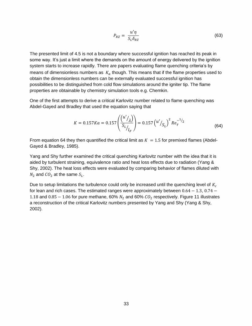
Yang and Shy further examined the critical quenching Karlovitz number with the idea that it is
aided by turbulent straining, equivalence ratio and heat loss effects due to radiation (Yang &
Shy, 2002). The heat loss effects were evaluated by comparing behavior of flames diluted with
and at the same .
Due to setup limitations the turbulence could only be increased until the quenching level of
for lean and rich cases. The estimated ranges were approximately between ,
and for pure methane, 60% and 60% respectively. Figure 11 illustrates
a reconstruction of the critical Karlovitz numbers presented by Yang and Shy (Yang & Shy,
2002).
34
Figure 11. Reconstruction of the global quenching results found by (Yang & Shy, 2002).
0
5
10
15
20
25
30
0,56 0,76 0,96 1,16 1,36
Kcr
it
Equivalence ratio
Pure Methane
60% N2
60% CO2

35
4 Methodology When studying ignition performance for a specific combustion application there’s mainly two
ways to go: direct measurements or computational fluid dynamics. By applying the concept of
ignition prediction through a critical Karlovitz number as presented by e.g. (Soworka, et al.,
2014) cost efficient ignition predictions may be obtained by CFD simulations. Evaluation of such
models is thus of interest which together with the ignition tests performed by (Berg, 2012)
constituted a base for evaluating the models on SIT’s ACR.
Geometrical models of the ACR were available from earlier studies made on that rig. However
this was a pilot project when it comes to the sequence of ignition thereby the theory of ignition
needed to be considered when deciding how to evaluate ignition from cold flow simulations. The
first step was thus to take the existing model and add a few surfaces bounding the
interesting region around the igniter tip. Figure 12 displays the four spheres added to the
geometry, the smallest surface is not visible though since it’s hidden inside the slightly bigger
sphere.
Figure 12. Interfaces bounding the spherical region, up to 2 cm in diameter, around the igniter tip.
The radius of the spheres was in some way randomly chosen. A base from Berg’s calculations
of quenching distance and some respect to the ability to mesh the spheres in a practical sense
were though considered when choosing 2, 2.5, 5 and 10 mm radiuses. The idea behind the
strategy to extend the ignition region in these “onion layers” comes from the expression of the
flow affected quenching distance. From equation 61 conclusions can be made that a very time
consuming iterative process would be required for every fuel if the spheres should have been
optimized to the quenching distance. Some more general surfaces were thus applied so the
prediction of ignition could be evaluated in subsequent steps from the same simulation.

36
The reason that the two biggest surfaces are split into two parts is that the ignition point is very
close to the periodic planes of the combustor chamber and those surfaces, together with the
rest of the model, was thus connected by cylindrical periodicity around the centerline. The first
half of the combustor chamber in Figure 12, were the ignition volumes are located, is the
volume referred to as the combustor chamber average later in the results.
4.1 Grid generation The procedure when creating a domain where the numerical computations can be performed is
called grid generation or meshing. Surfaces and internal volumes of the geometry are then
divided or discretized into a number of cells that may be of different geometrical shape. All mesh
created in this thesis has consisted of triangular/Tetrahedral structures. The utilized software for
creating all mesh was ANSYS ICEM version 15.0.
To distinguish that a final CFD solution is independent of the mesh size a so called grid study is
mandatory for reliable results. A grid study is performed by creating a couple of mesh, going
from course to finer, and then run the same case while evaluating a few relevant parameters to
evaluate how the results varies with respect to mesh size. Four mesh of approximately
and million cells where created for the purpose of performing a grid study for the analyzed
cases. Figure 13 illustrates the surface mesh created and used for all 4 volume mesh used in
the grid study.
Figure 13. Surface mesh, the base of all four mesh tested.
Figure 14 displays a cut plane for the 6 million volume mesh that has its normal in the z
direction. Its location is set in line with one of the pilot outlets. The main difference between the
four created mesh is refinements of the pilot nozzles, the burner outlet and the flow path
towards the ignition point.
37
Figure 14. Cut plane of the 6 million cell volume mesh.
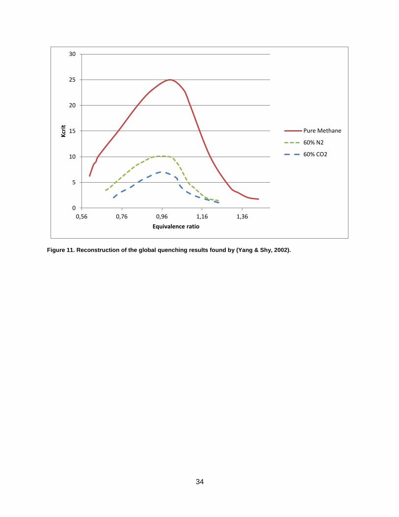
4.1.1 Mesh quality
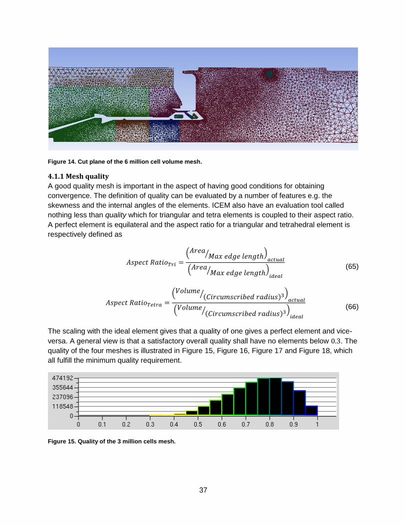
A good quality mesh is important in the aspect of having good conditions for obtaining
convergence. The definition of quality can be evaluated by a number of features e.g. the
skewness and the internal angles of the elements. ICEM also have an evaluation tool called
nothing less than quality which for triangular and tetra elements is coupled to their aspect ratio.
A perfect element is equilateral and the aspect ratio for a triangular and tetrahedral element is
respectively defined as
( ⁄ )
( ⁄ )
(65)
( ⁄ )
( ⁄ )
(66)
The scaling with the ideal element gives that a quality of one gives a perfect element and vice-
versa. A general view is that a satisfactory overall quality shall have no elements below . The
quality of the four meshes is illustrated in Figure 15, Figure 16, Figure 17 and Figure 18, which
all fulfill the minimum quality requirement.
Figure 15. Quality of the 3 million cells mesh.

38
Figure 16. Quality of the 6 million cells mesh.
Figure 17. Quality of the 10 million cells mesh.
Figure 18. Quality of the 15 million cells mesh.
4.2 Pre processing In the pre-processing of a simulation the physical properties of a specific case is set. Material
properties, boundary conditions, initial conditions and physical models are a few settings
controlled by the user and the pre-processer and solver mainly used in this thesis were ANSYS
CFX 14.5. Table 5 and Table 6 summarize the settings used in this thesis.
Table 5. Pre-processor settings.

39
Table 6. Solver control settings.
4.3 Post processing Analysis of the results obtained from the simulations is called post processing and was done
using CFX-post and Microsoft Excel.
4.4 Chemical simulations in GENE-AC GENE-AC is a Siemens in house code for solving complex chemical kinetic problems (Marashi,
2013). The program can with benefit be used in combustion applications and the program has a
pre-defined toolbox for both NOx prediction and flame calculation. The flame calculation model
utilizes a one dimensional flame reactor where the fuel/air mixture is assumed to be fully
premixed. The settings needed to be set are then which reaction scheme shall be used,
pressure, range of equivalence ratios solved for, temperature and composition of fuel and
oxidizer. The settings used for the chemical simulations in GENE-AC are shown in Table 7.
Table 7. GENE-AC settings.
4.4.1 Laminar flame speed and flame thickness
The flame calculations in GENE-AC resulted in achieving data of the laminar flame speed as a
function of the equivalence ratio. The simulations also gave data of how the fraction of different
chemical species changed along the axial direction of the planar laminar flame, from that data
concentration plots like Figure 19 may be obtained.

40
Figure 19. Mole fraction and temperature profile as a function of distance in the axial flame direction, equivalence ratio 0.98. Fuel composition of 80% CH4 and 20% CO2
Equation 49 and 50 can then be applied to plots as Figure 19 which finally results in data of
flame thickness and reaction zone thickness as functions of equivalence ratios. Figure 20 and
Figure 21 represents the flame thickness and RZ thickness obtained by the procedure
mentioned above. Even though the data shows a smooth trend the fitted polynomial is slightly
overcompensating. The trend line used was though the best possible and from the CFD
simulations conclusions that the most important area is for low equivalence ratios which further
justify the chosen polynomial.
0
500
1000
1500
2000
2500
0
0,1
0,2
0,3
0,4
0,5
0,6
0,7
0,8
0 0,005 0,01 0,015 0,02
Tem
pe
ratu
re [
K]
Mo
lefr
acti
on
[m
ole
/mo
le]
distance [m]
[N2] [CH4] [CO] [CO2] [O2] [OH] [H20] Temperature

41
Figure 20. Flame thickness as a function of the equivalence ratio. Fuel composition of 80% CH4 and 20% CO2
Figure 21. Reaction zone thickness as a function of the equivalence ratio. Fuel composition of 80% CH4 and 20% CO2
4.5 Ignition evaluation The overall procedure tested for evaluating ignition incorporates all steps presented above in
section four. The general idea is to be able to simulate how the Karlovitz number changes in the
ignition volumes added around the igniter tips. By comparing the Karlovitz number in those
regions to data of critical Karlovitz numbers in the sense of flame extinction the possibilities of
flame kernel growth can be evaluated. If the kernel reaches its critical size then ignition is
determined successful. This approach disregards the last propagation step of the flame kernel
igniting the whole combustion chamber and is thus a simplification of the ignition sequence. To
0
0,001
0,002
0,003
0,004
0,005
0,006
0,007
0,008
0,009
0 0,5 1 1,5 2
Lam
inar
Th
ickn
ess
[m
]
Equivalence Ratio
Laminar thickness
0
0,0005
0,001
0,0015
0,002
0,0025
0 0,5 1 1,5 2
RZ
Thic
kne
ss [
m]
Equivalence Ratio
RZ thickness

42
obtain the Karlovitz number for the evaluated ignition surfaces the results of the cold flow and
the chemical simulations is combined in the post processing programs.
Similar attempts to predict ignition from cold flow simulations has previous been made
(Neophytou, et al., 2012) (Soworka, et al., 2014). The approach has been slightly different
though and the modeling of the final step in the ignition sequence has been more sophisticated.
Their approach has been to develop a code creating a mesh with arbitrary cell size where every
cell is assigned properties as Karlovitz number and flow parameters obtained from the cold flow
simulations made. From comparison of the critical Karlovitz number to the Karlovitz number in
each cell they’re given a state of either extinguishable or burnable. A specific volume,
representing the spark volume, is then put into combustible mode and the particles in the
affected cells starts a sort of random walk following the streamlines of the local flow field. If a
particle reaches a cell in the burnable state it switches to combustible and the particle in that cell
will start its own random walk and if a particle meets a cell in the cold state it extinguishes. After
a specific time the ratio of number of cells in the combustible state to the total number of cells is
evaluated and if this number is higher than a pre-set limit the ignition is deemed successful. The
coding of this last step is though relatively complicated and not within the frames for this thesis
but there would be no problem to implement it in a later stage of the research.

43
5 Results of pre-studies
5.1 GENE-AC results and validation The results obtained by GENE-AC and the GriMech 3.0 reaction scheme are primarily the
laminar flame speed, flame thickness (Figure 20) and the reaction zone thickness (Figure 21).
What’s important is to validate the results against some source presenting measurements of
these properties for similar conditions. Dahoe and de Goey (Dahoe & de Goey, 2003) presented
a model to determine the laminar flame speed and the flame thickness via gas explosions in
closed vessels (combustion bomb tests). They then compared their results to observed data for
those parameters depending on equivalence ratio, pressure and temperature. The mean trend
of these data where then collected to be compared to the results of the GENE-AC simulations.
Figure 22 compares the laminar flame speed for pure methane combustion and even though the
range of the measured data is not as large as the simulated results both the trend and the
absolute values of the two curves are in good agreement.
Figure 22. Average measured laminar flame speed presented in Dahoe & de Goey (Dahoe & de Goey, 2003) compared to results from GENE-AC for pure methane.
Figure 23, Figure 24, Figure 25 and Figure 26 presents the influence increased fractions of inert
gases has on the laminar flame speed, flame thickness and reaction zone thickness according
to GENE-AC. The laminar flame speed is decreased for all equivalence ratios and fuel
compositions when the amount of inert gases is increased the maximum flame speed is also
shifted towards lower equivalence ratios. The flame and RZ thickness shows a trend of
decreasing thickness for increased amounts of inert gases. The influence from the inert gases
are however small except at equivalence ratios above ~1.2 where the different fuel
compositions show more distinct differences relative each other.
0
5
10
15
20
25
30
35
40
0 0,2 0,4 0,6 0,8 1 1,2 1,4 1,6
Lam
inar
fla
me
sp
ee
d [
cm/s
]
equivalent ratio
(Dahoe and de Goey, 2003) GeneAC GRI30
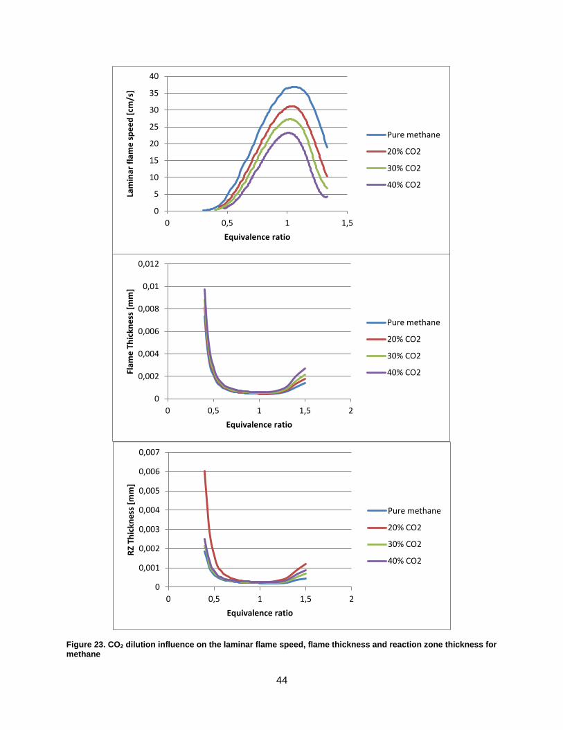
44
Figure 23. CO2 dilution influence on the laminar flame speed, flame thickness and reaction zone thickness for methane
0
5
10
15
20
25
30
35
40
0 0,5 1 1,5
Lam
inar
fla
me
sp
ee
d [
cm/s
]
Equivalence ratio
Pure methane
20% CO2
30% CO2
40% CO2
0
0,002
0,004
0,006
0,008
0,01
0,012
0 0,5 1 1,5 2
Flam
e T
hic
kne
ss [
mm
]
Equivalence ratio
Pure methane
20% CO2
30% CO2
40% CO2
0
0,001
0,002
0,003
0,004
0,005
0,006
0,007
0 0,5 1 1,5 2
RZ
Thic
kne
ss [
mm
]
Equivalence ratio
Pure methane
20% CO2
30% CO2
40% CO2
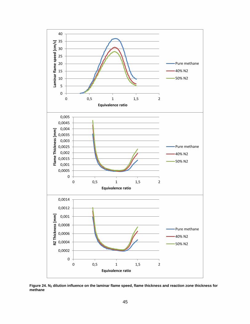
45
Figure 24. N2 dilution influence on the laminar flame speed, flame thickness and reaction zone thickness for methane
0
5
10
15
20
25
30
35
40
0 0,5 1 1,5 2
Lam
inar
fla
me
sp
ee
d [
cm/s
]
Equivalence ratio
Pure methane
40% N2
50% N2
0
0,0005
0,001
0,0015
0,002
0,0025
0,003
0,0035
0,004
0,0045
0,005
0 0,5 1 1,5 2
Flam
e T
hic
kne
ss [
mm
]
Equivalence ratio
Pure methane
40% N2
50% N2
0
0,0002
0,0004
0,0006
0,0008
0,001
0,0012
0,0014
0 0,5 1 1,5 2
RZ
Thic
kne
ss [
mm
]
Equivalence ratio
Pure methane
40% N2
50% N2
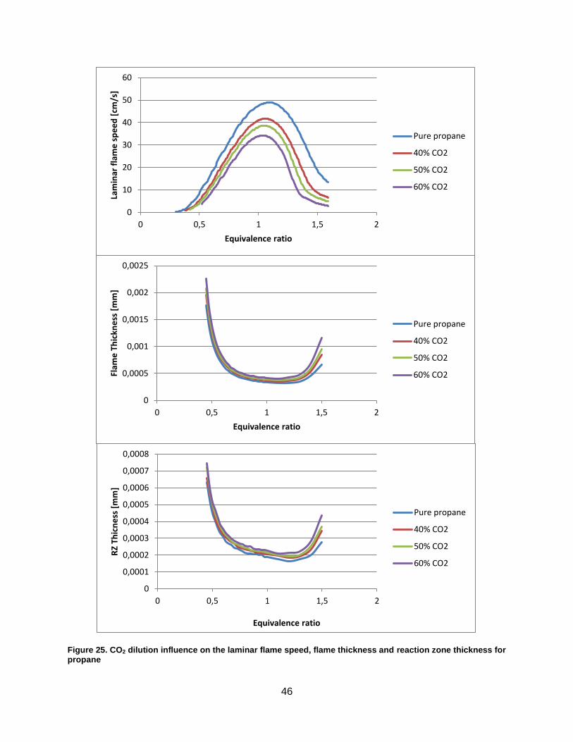
46
Figure 25. CO2 dilution influence on the laminar flame speed, flame thickness and reaction zone thickness for propane
0
10
20
30
40
50
60
0 0,5 1 1,5 2
Lam
inar
fla
me
sp
ee
d [
cm/s
]
Equivalence ratio
Pure propane
40% CO2
50% CO2
60% CO2
0
0,0005
0,001
0,0015
0,002
0,0025
0 0,5 1 1,5 2
Flam
e T
hic
kne
ss [
mm
]
Equivalence ratio
Pure propane
40% CO2
50% CO2
60% CO2
0
0,0001
0,0002
0,0003
0,0004
0,0005
0,0006
0,0007
0,0008
0 0,5 1 1,5 2
RZ
Thic
ne
ss [
mm
]
Equivalence ratio
Pure propane
40% CO2
50% CO2
60% CO2

47
Figure 26. N2 dilution influence on the laminar flame speed, flame thickness and reaction zone thickness for propane
0
10
20
30
40
50
60
0 0,5 1 1,5 2
Lam
inar
fla
me
sp
ee
d [
cm/s
]
Equivalence ratio
Pure propane
60% N2
70% N2
75% N2
0
0,0002
0,0004
0,0006
0,0008
0,001
0,0012
0,0014
0,0016
0 0,5 1 1,5 2
Flam
e T
hic
kne
ss [
mm
]
Equivalence ratio
Pure propane
60% N2
70% N2
75% N2
0
0,0001
0,0002
0,0003
0,0004
0,0005
0,0006
0 0,5 1 1,5 2
RZ
Thic
kne
ss [
mm
]
Equivalence ratio
Pure propane
60% N2
70% N2
75% N2

48
Figure 27 compares the flame thickness calculated by equation 49 for pure methane to the
summation of several measured data presented in Dahoe and de Goey (Dahoe & de Goey,
2003). In absolute numbers the two curves are a bit off, the trend they show is though similar
and in general the simulated result is just displaced slightly in a south-west direction.
Figure 27. Average measured flame thickness presented in Dahoe and de Goey (Dahoe & de Goey, 2003) compared to results from GENE-AC for pure methane.
Stone et al. made measurements on how dilution of inert gases in a combustible mixture
affected the laminar burning velocity (Stone, et al., 1998). The data from their measurements
where then extracted for comparison with the results of the GENE-AC simulations, Figure 28
and Figure 29. It shall be noted that the data represents flames at an equivalence ratio of 1.05,
normal temperature and pressure.
Figure 28 displays a very good correlation for GENE-AC towards the measured data. The
GENE-AC results for the simulations, Figure 29, shows slight less correlation towards the
measured data presented by Stone et al. (Stone, et al., 1998). GENE-AC seems to under
estimate the flame speed for lower fractions of both N2 and CO2. The results than seems to shift
towards over estimation when passing a mole fraction of around 20 and 40 mole% N2 and CO2
respectively.
0
2
4
6
8
10
12
0 0,5 1 1,5 2
Flam
e T
hic
kne
ss [
mm
]
Equivalence Ratio
(Dahoe and de Goey,2003)
(GeneAC)

49
Figure 28. The effect that increased amount of CO2 has on the laminar flame speed for methane based fuel, comparison of measured (Stone, et al., 1998) and simulated results.
Figure 29. The effect that increased amount of N2 has on the laminar flame speed for methane based fuel, comparison of measured (Stone, et al., 1998) and simulated results.
It shall be noted that small parts of both the similarities and the dissimilarities may be due to the
manual extraction of the measured data. Some loss in accuracy always appears without more
sophisticated tools than a ruler, paint and excel.
An earlier master thesis at SIT made by Marashi evaluated the prediction accuracy of the
laminar flame speed for GENE-AC utilizing both the GriMech 3.0 and the LOGE-28 reaction
scheme (Marashi, 2013). Figure 30 shows an evaluation of methane mixed with CO2 made by
Marashi and it shows good prediction for equivalence ratios roughly between 0.8 and 1.1

50
(Marashi, 2013). For higher equivalence ratios GENE-AC underestimates the flame speed
relative measured results. From the methane/CO2 validation in Figure 28 GENE-AC predicts the
flame speed very accurate for a CO2 fraction of 35.6 mole%. For the data presented by Marashi
in Figure 30 GENE-AC shows a small underestimation.
Figure 30. Laminar flame speed for methane mixed with 35.6 mole% CO2 data simulated with GENE-AC and measured data is presented for comparison, presented by Marashi (Marashi, 2013).
The general conclusion from Marashi when using the GriMech 3.0 reaction scheme was that
good agreement were obtained for methane while for propane the laminar flame speed was
consequently overestimated (Marashi, 2013), Figure 31 displays this.

51
Figure 31. Comparison of laminar flame speed data for propane simulated with GENE-AC and measured data Presented by Marashi (Marashi, 2013).
Table 8 presents a rough estimation of the data presented in Figure 31 and the overestimation
from GENE-AC goes between 21.7% and 37.5%. However the measured data for an
equivalence ratio of 0.9 has relative big difference and shall maybe be left out when putting
some kind of general overestimation. Taking the average for the other equivalence ratios yields
a general overestimation of 26.3%.
Table 8. Extraction of laminar flame speed data for measured and simulated cases presented in Figure 31.
Eq Hassan Jomaas GRIMech 3.0-GENE-AC Jomaas ratio Hassan ratio
0.8 29 29 37 1.276 1.276 0.9 32 36 44 1.222 1.375 1 40 41.5 50.5 1.217 1.263
1.1 40 41.7 52 1.247 1.300
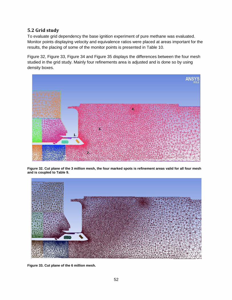
52
5.2 Grid study To evaluate grid dependency the base ignition experiment of pure methane was evaluated.
Monitor points displaying velocity and equivalence ratios were placed at areas important for the
results, the placing of some of the monitor points is presented in Table 10.
Figure 32, Figure 33, Figure 34 and Figure 35 displays the differences between the four mesh
studied in the grid study. Mainly four refinements area is adjusted and is done so by using
density boxes.
Figure 32. Cut plane of the 3 million mesh, the four marked spots is refinement areas valid for all four mesh and is coupled to Table 9.
Figure 33. Cut plane of the 6 million mesh.
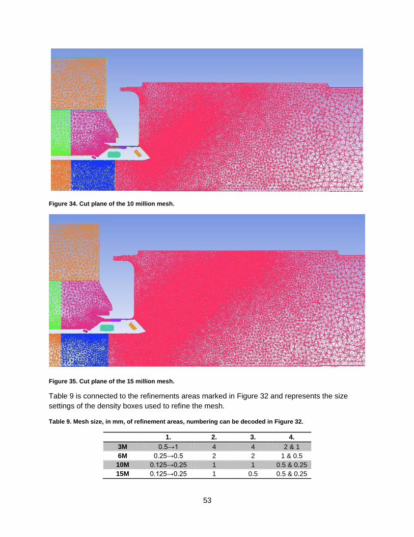
53
Figure 34. Cut plane of the 10 million mesh.
Figure 35. Cut plane of the 15 million mesh.
Table 9 is connected to the refinements areas marked in Figure 32 and represents the size
settings of the density boxes used to refine the mesh.
Table 9. Mesh size, in mm, of refinement areas, numbering can be decoded in Figure 32.
1. 2. 3. 4.
3M 0.5→1 4 4 2 & 1
6M 0.25→0.5 2 2 1 & 0.5
10M 0.125→0.25 1 1 0.5 & 0.25
15M 0.125→0.25 1 0.5 0.5 & 0.25
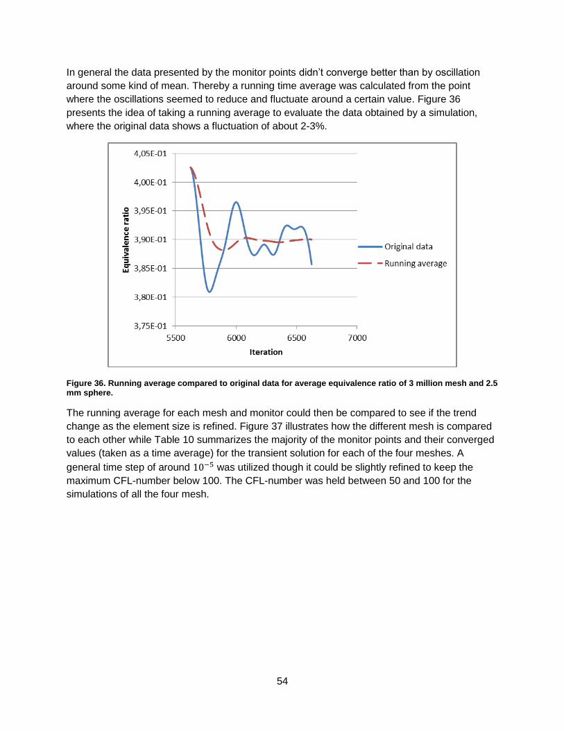
54
In general the data presented by the monitor points didn’t converge better than by oscillation
around some kind of mean. Thereby a running time average was calculated from the point
where the oscillations seemed to reduce and fluctuate around a certain value. Figure 36
presents the idea of taking a running average to evaluate the data obtained by a simulation,
where the original data shows a fluctuation of about 2-3%.
Figure 36. Running average compared to original data for average equivalence ratio of 3 million mesh and 2.5 mm sphere.
The running average for each mesh and monitor could then be compared to see if the trend
change as the element size is refined. Figure 37 illustrates how the different mesh is compared
to each other while Table 10 summarizes the majority of the monitor points and their converged
values (taken as a time average) for the transient solution for each of the four meshes. A
general time step of around was utilized though it could be slightly refined to keep the
maximum CFL-number below 100. The CFL-number was held between 50 and 100 for the
simulations of all the four mesh.

55
Figure 37. Mesh comparison of running average for equivalence ratio of 2.5 mm sphere.
From Table 10 monitor point 1, 2, 4 and 8 can be deemed to be independent of mesh size
refinements since they’re fairly constant between all four mesh. Monitor point 3, 5, 6 and 7 show
more significant fluctuations between the four meshes though. This indicates that the most
coarse mesh of 3 million elements is unsatisfactory for having good results in the parameter
study. Especially the equivalence ratio within the added surfaces around the ignition point is
important for the further analysis and therefore the three and 6 million can be disregarded from
further studies. Due to computational time competiveness and small differences between the 10
and 15 million meshes the 10 million are considered as the most suitable mesh for the rest of
the studies.
Table 10. Summation of monitor data for each of the four mesh, data is presented as percentage of the 15 million mesh values.
Monitor point 3 million cells
6 million cells
10 million cells
15 million cells
1. Velocity ignition point [m/s] 0.99 1.01 0.99 1.00 2. Velocity at burner outlet, 2/3 r from centrum [m/s] 0.99 1.01 1.00 1.00 3. Average velocity pilot nozzle [m/s] 0.89 0.97 1.01 1.00 4. Velocity burner outlet, center [m/s] 1.00 1.03 1.01 1.00 5. Gas velocity at smallest section of the pilot fuel system [m/s] 0.98 1.01 1.00 1.00 6. Average equivalence ratio of 2.5 mm r sphere 1.29 1.24 1.02 1.00 7. Average equivalence ratio of 10 mm r sphere 1.28 1.23 1.00 1.00 8. Average equivalence ratio combustor chamber 1.02 1.04 0.98 1.00

56
To further strengthen the mesh choice based on the monitor points different velocity profiles of
the burner can be compared. Figure 38 displays the time averaged velocity profile of each
simulated mesh. The scale is adjusted to the local maximum and minimum of the plane which
benefits comparison of the pilot nozzle activity which by far is exposed to the highest velocities.
In general the trend of the pilot nozzle jet is similar between all four mesh, the jet is in all cases
somewhat curved around the nozzle outlet. Though from the 6 million mesh a small separation
of the jet starts to appear and the pattern of one more downward portion of the jet is more or
less identical for the 10 and 15 million meshes. This supports the choice of the 10 million mesh.
Figure 38. Time averaged velocity profiles of all four meshes. The figure is organized with the smallest mesh at the top left corner and increases from 3 to 15 million in a z-pattern.
In Figure 39 the velocity scale has been constrained to a maximum of twice the average velocity
of the end of the mixing tube which aids mesh independency evaluation of areas of lower
velocity. As a consequence the pilot jet velocity profile looks more homogenous even though it’s
not the case. The more detailed distinctions of the burner jet highlight a slight difference in how
fast the centrum velocity of the jet homogenize. From Figure 39 it can also be deduced that the

57
stagnation point is basically at an identical location for all mesh. Still the mesh dependency
seems to level out from the 10 million mesh.
Figure 39. Time averaged velocity profiles with adjusted velocity scale. The figure is organized with the smallest mesh at the top left corner and increases from 3 to 15 million in a z-pattern. The part of the yellow “star” pointing out of the normal displays the planar coordinates of the ignition point.
Figure 40 compares velocities along a vertical line through the ignition point where the trend
changes slightly after refining the 6 million cell mesh.
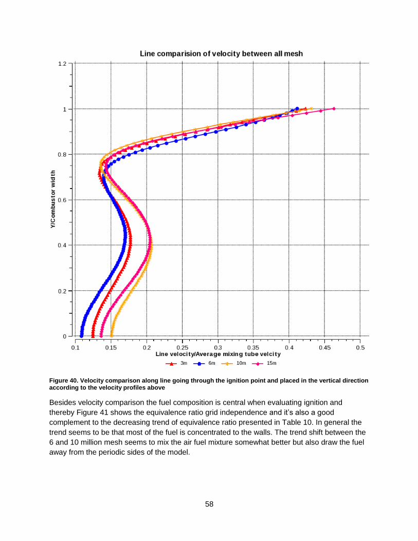
58
Figure 40. Velocity comparison along line going through the ignition point and placed in the vertical direction according to the velocity profiles above
Besides velocity comparison the fuel composition is central when evaluating ignition and
thereby Figure 41 shows the equivalence ratio grid independence and it’s also a good
complement to the decreasing trend of equivalence ratio presented in Table 10. In general the
trend seems to be that most of the fuel is concentrated to the walls. The trend shift between the
6 and 10 million mesh seems to mix the air fuel mixture somewhat better but also draw the fuel
away from the periodic sides of the model.
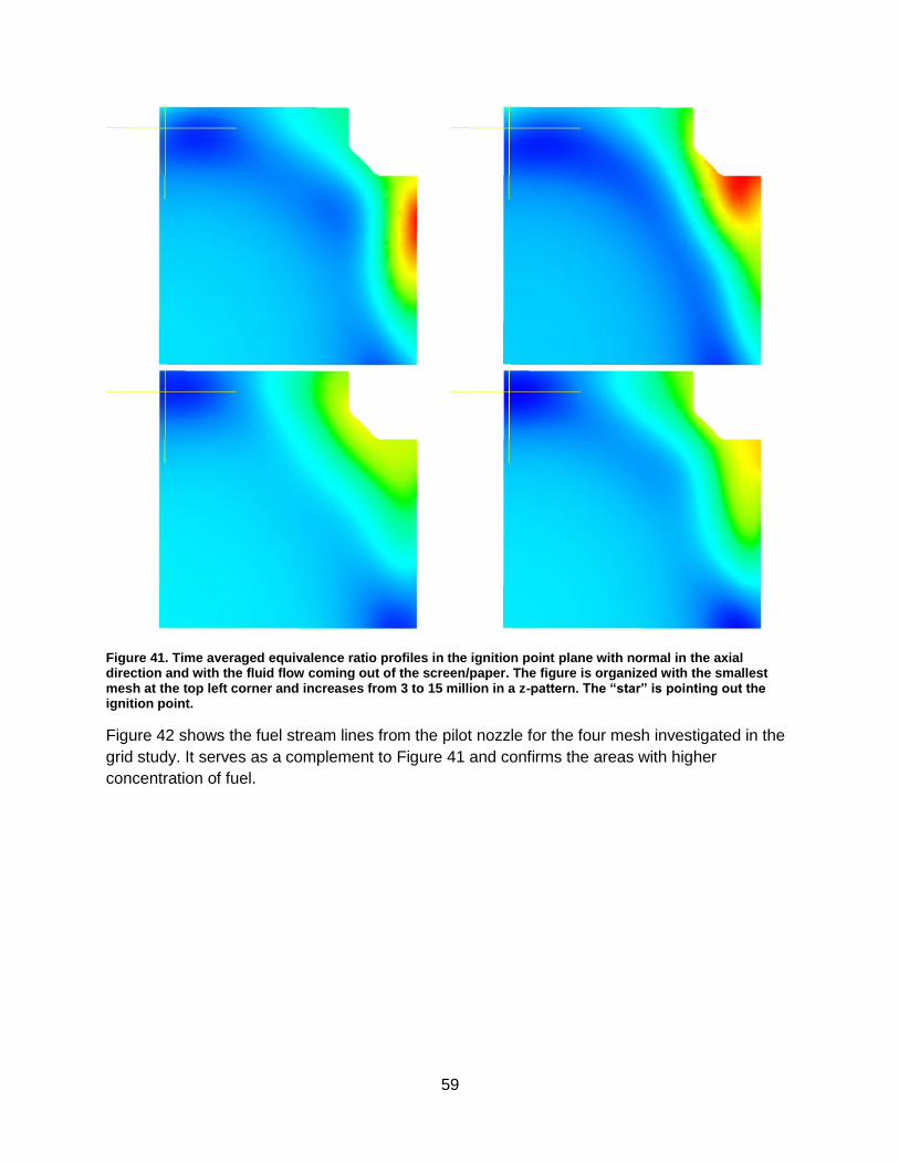
59
Figure 41. Time averaged equivalence ratio profiles in the ignition point plane with normal in the axial direction and with the fluid flow coming out of the screen/paper. The figure is organized with the smallest mesh at the top left corner and increases from 3 to 15 million in a z-pattern. The “star” is pointing out the ignition point.
Figure 42 shows the fuel stream lines from the pilot nozzle for the four mesh investigated in the
grid study. It serves as a complement to Figure 41 and confirms the areas with higher
concentration of fuel.

60
Figure 42. Fuel streamlines for pure methane, mesh size increases from 3 to 15 million in a z-pattern.
5.3 Comparison to Ansys Fluent To evaluate the difference between Ansys CFX and Ansys Fluent my friend and colleague
Dejan Korén used mesh and boundary conditions from this case and did a mesh study by
solving for the 3 million mesh and then split all cells to solve the refined 22 million mesh. His
results could then be used as an additional layer to this thesis where the results of the two
solvers could be compared. For further details of the method used the reader is referred to
search for his work from this preliminary reference (Korén, 2015).
The velocity profile presented by Figure 43 shows distinct differences especially when it comes
to the pilot fuel jet but also the stagnation point is further out for the CFX results. The distinction
between the two three million mesh runs (exactly the same mesh) and the distinction between
the 15 and 22 million mesh is similar. This means that the distinction isn’t due to the mesh since
the discrepancy between the two solvers is present even when the case is solved for the same
3 million mesh. The SST-turbulence model was utilized for both Ansys Fluent and CFX which
probably shouldn’t contribute to any bigger distinctions. According to Glenn Horrocs, a well-
respected guy at the CFD-online forum, the turbulence models are pretty much the same for
Ansys Fluent and CFX since they are provided by the same company (Horrocs, 2011). However

61
by inspection in the Ansys help manual differences in the applied constants for the SST
turbulence model in CFX and Fluent is noticed. This may thus be one of the reasons for the
discrepancies seen in Figure 43, Figure 44 and Figure 45. Discretization differences may also
be a part of the difference seen when comparing CFX and Fluent these effects shall however
disappear by using a mesh that is fine “enough”. It is hard to say if the 15 and 22 million mesh
respectively is fine enough to not be affected by discretization errors. Evaluating finer mesh than
these two was however limited by available computing resources. The influence from the
different turbulence model constants together with the possible discretization differences may
be two things to investigate if comparison of CFX and Fluent is interesting. This is however not
the scope of this thesis.
Figure 43. Time averaged velocity profiles of the periodic plane. Fluent results is presented at the left side of the figure and CFX result is presented on the right side, mesh elements increases in the downward direction.
Figure 44 compares the equivalence ratio in a plane located at the axial coordinate of the
ignition point. Some of the trends appearing when refining the mesh for both solvers seems to
be consistent e.g. that the zone of highest fuel concentration gets slightly leaner when refining
the mesh. This probably means that the mixing of the turbulence model is aided by a finer
mesh. Another notification to make from Figure 44 is that refining the mesh doesn’t narrow off
the high concentration area along the walls when using the Fluent solver. This can probably be
described by the pilot fuel jets that show significant distinction.

62
Figure 44. Time averaged equivalence ratio profiles in the ignition point plane with normal in the axial direction and with the fluid flow coming out of the screen/paper. Fluent results is presented at the left side of the figure and CFX result is presented on the right side, mesh elements increases in the downward direction.
Figure 45 shows the fuel stream lines from the pilot nozzle coupled to Figure 44. It serves as a
complement to confirm differences seen in Figure 45 and approve the areas with higher
concentration of fuel.
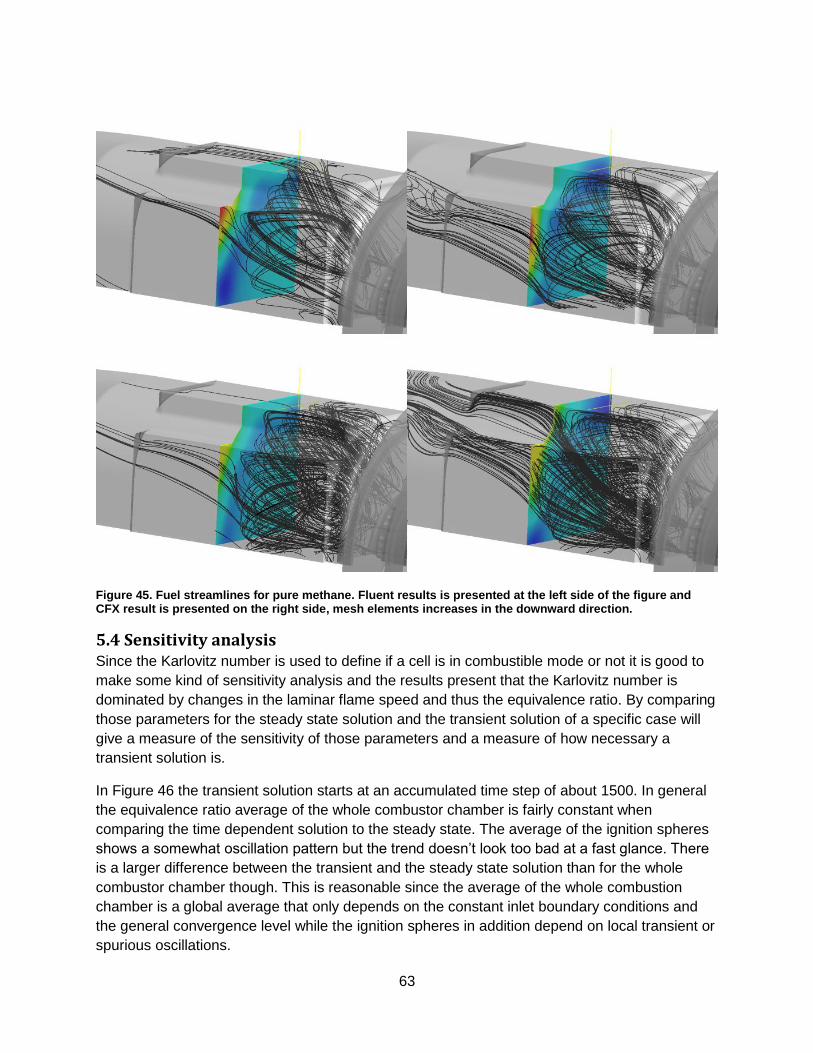
63
Figure 45. Fuel streamlines for pure methane. Fluent results is presented at the left side of the figure and CFX result is presented on the right side, mesh elements increases in the downward direction.
5.4 Sensitivity analysis Since the Karlovitz number is used to define if a cell is in combustible mode or not it is good to
make some kind of sensitivity analysis and the results present that the Karlovitz number is
dominated by changes in the laminar flame speed and thus the equivalence ratio. By comparing
those parameters for the steady state solution and the transient solution of a specific case will
give a measure of the sensitivity of those parameters and a measure of how necessary a
transient solution is.
In Figure 46 the transient solution starts at an accumulated time step of about 1500. In general
the equivalence ratio average of the whole combustor chamber is fairly constant when
comparing the time dependent solution to the steady state. The average of the ignition spheres
shows a somewhat oscillation pattern but the trend doesn’t look too bad at a fast glance. There
is a larger difference between the transient and the steady state solution than for the whole
combustor chamber though. This is reasonable since the average of the whole combustion
chamber is a global average that only depends on the constant inlet boundary conditions and
the general convergence level while the ignition spheres in addition depend on local transient or
spurious oscillations.
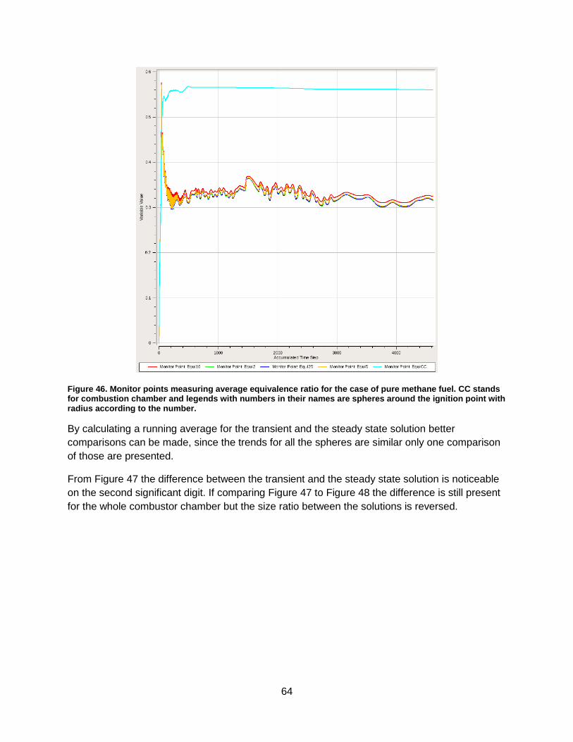
64
Figure 46. Monitor points measuring average equivalence ratio for the case of pure methane fuel. CC stands for combustion chamber and legends with numbers in their names are spheres around the ignition point with radius according to the number.
By calculating a running average for the transient and the steady state solution better
comparisons can be made, since the trends for all the spheres are similar only one comparison
of those are presented.
From Figure 47 the difference between the transient and the steady state solution is noticeable
on the second significant digit. If comparing Figure 47 to Figure 48 the difference is still present
for the whole combustor chamber but the size ratio between the solutions is reversed.
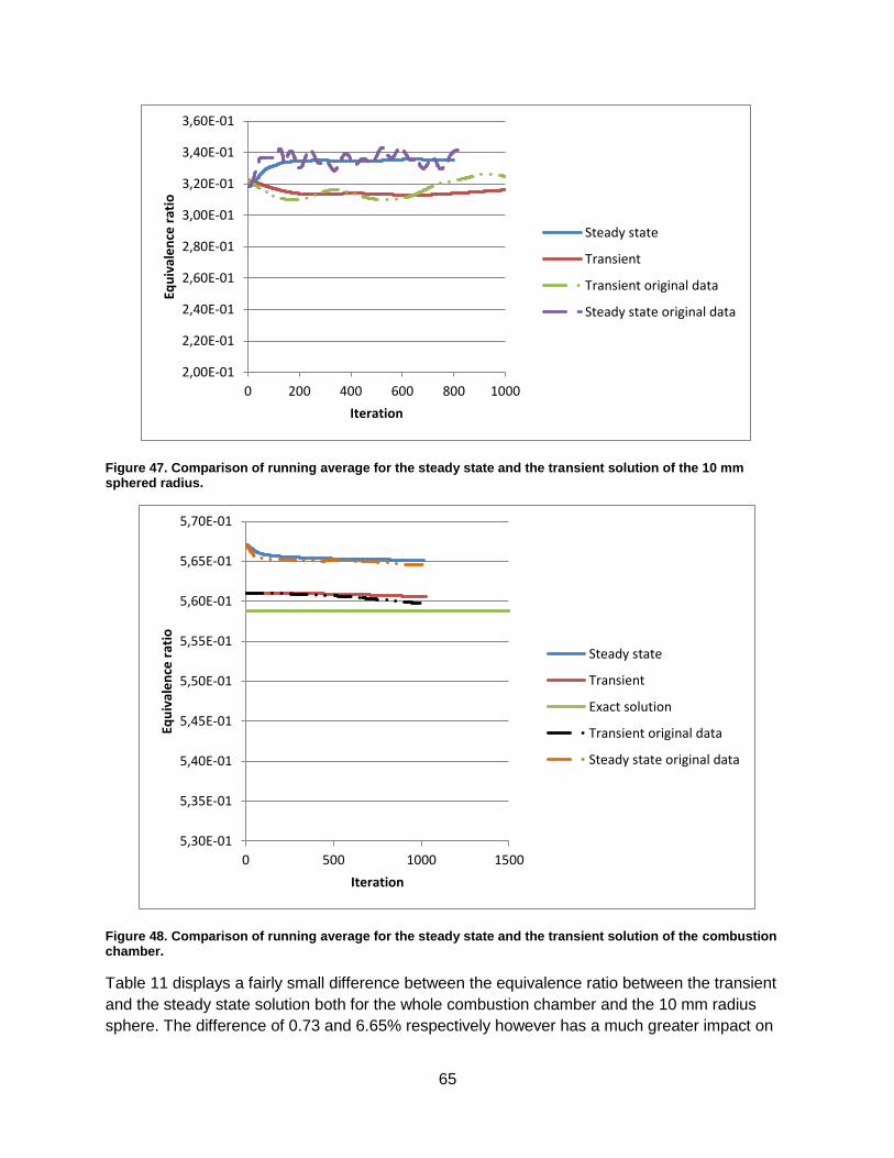
65
Figure 47. Comparison of running average for the steady state and the transient solution of the 10 mm sphered radius.
Figure 48. Comparison of running average for the steady state and the transient solution of the combustion chamber.
Table 11 displays a fairly small difference between the equivalence ratio between the transient
and the steady state solution both for the whole combustion chamber and the 10 mm radius
sphere. The difference of 0.73 and 6.65% respectively however has a much greater impact on
2,00E-01
2,20E-01
2,40E-01
2,60E-01
2,80E-01
3,00E-01
3,20E-01
3,40E-01
3,60E-01
0 200 400 600 800 1000
Equ
ival
en
ce r
atio
Iteration
Steady state
Transient
Transient original data
Steady state original data
5,30E-01
5,35E-01
5,40E-01
5,45E-01
5,50E-01
5,55E-01
5,60E-01
5,65E-01
5,70E-01
0 500 1000 1500
Equ
ival
en
ce r
atio
Iteration
Steady state
Transient
Exact solution
Transient original data
Steady state original data
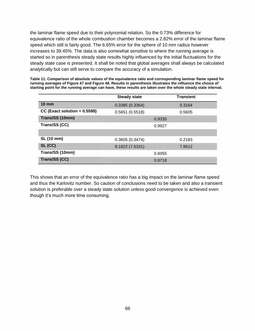
66
the laminar flame speed due to their polynomial relation. So the 0.73% difference for
equivalence ratio of the whole combustion chamber becomes a 2.82% error of the laminar flame
speed which still is fairly good. The 6.65% error for the sphere of 10 mm radius however
increases to 39.45%. The data is also somewhat sensitive to where the running average is
started so in parenthesis steady state results highly influenced by the initial fluctuations for the
steady state case is presented. It shall be noted that global averages shall always be calculated
analytically but can still serve to compare the accuracy of a simulation.
Table 11. Comparison of absolute values of the equivalence ratio and corresponding laminar flame speed for running averages of Figure 47 and Figure 48. Results in parenthesis illustrates the influence the choice of starting point for the running average can have, these results are taken over the whole steady state interval.
Steady state Transient
10 mm 0.3385 (0.3364) 0.3164
CC (Exact solution = 0.5588) 0.5651 (0.5518) 0.5605
Trans/SS (10mm) 0.9335
Trans/SS (CC) 0.9927
SL (10 mm) 0.3605 (0.3474) 0.2183
SL (CC) 8.1822 (7.5331) 7.9512
Trans/SS (10mm) 0.6055
Trans/SS (CC) 0.9718
This shows that an error of the equivalence ratio has a big impact on the laminar flame speed
and thus the Karlovitz number. So caution of conclusions need to be taken and also a transient
solution is preferable over a steady state solution unless good convergence is achieved even
though it’s much more time consuming.

67
6 Evaluation of ignition model From equation 64 mainly three parameters affects the Karlovitz number and thus the prediction
of ignition limits. These parameters are the RMS velocity, kinematic viscosity and the laminar
flame speed that is connected to the equivalence ratio and thus the mixing of the flow. Table 12
summarizes the average and the ratio of the standard deviation and the average for the
Karlovitz affecting parameters for each fuel group. This can be translated to how much each
parameter is affected when changing the amount of inert gases and thereby it tells how much
each of the parameters affects the Karlovitz number and thereby the predicted ignition limit. All
parameters are evaluated on a global scale which means that their affect is calculated from an
average of the whole combustor chamber and not only close to the igniter which would be a
very CFD-dependent result. So by using the assumption that the combustion chamber is
perfectly mixed in reality a more rigid impact study can be calculated. It shall be noted that the
RMS velocity is hopeless to calculate without using CFD so thereby the CFD simulations was
used to get a grip of its combustion chamber average and then its effect was slightly
overestimated. That’s also why the ratio of the standard deviation and the average is constant
for all four fuel groups.
A short evaluation shows that the RMS velocity varies about 8 % between all fuel composition
cases, the kinematic viscosity varies less than 1% and the laminar flame speed varies between
29-94%. This concludes that the RMS velocity probably have some effect on the predicted
ignition limits but in general it’s the laminar flame speed and thus the equivalence ratio that
mainly demand the ignition limits using the Karlovitz number.
Table 12. Average and the ratio between the standard deviation and the average for the parameters that affects the Karlovitz number. Values are calculated with the assumption of a perfectly premixed combustor chamber except for the RMS velocity where CFD-results are used with the assumption of correct simulated velocity field.
Global values
1.5
Methane/CO2 1.5
Methane/N2 0.5
Methane/CO2
0.5
Methane/N2
SL2
Methane/CO2 SL
2
Methane/N2
Ave 2.04 1.95 4.68E-03 4.72E-03 29.17 46.84
Stdev/Ave ~8% ~8% 0.543% 0.121% 81.902% 28.883%
1.5
Propane/CO2 1.5
Propane/N2 0.5
Propane/CO2
0.5
Propane/N2
SL2
Propane/CO2 SL
2
Propane/N2
Ave 1.99 2.02E 4.59E-03 4.63E-03 23.81 40.22
Stdev/Ave ~8% ~8% 0.398% 0.158% 93.648% 29.320%
From the assumption that the equivalence ratio and the rest of the parameters of the
combustion chamber is homogenous the ignition limit can be estimated. Since Berg’s tests
where made under constant energy flow the perfectly mixed equivalence ratio is constant as
long as the same fuel base of methane (0.559) or propane (0.508) is used. Table 13 and Table
14 on the next page presents the ignition limits predicted without the influence of CFD-
simulations. The simulations contribute a little to the result by providing the average RMS
velocity of the combustor chamber for each fuel group but that’s somehow unavoidable. Also
since the RMS velocity show fairly small fluctuations between each fuel case compared to the

68
laminar flame speed it’s somehow justified to assume them as constant at their average
obtained by Ansys CFX. By comparing the Karlovitz numbers of Table 13 and Table 14 towards
the critical Karlovitz number of 1.5 no fuel composition shall be able to ignite not even the pure
methane or propane which indeed is possible to use for ignition. A conclusion from this could be
that the air to fuel ratio is richer than the combustion chamber average in the igniter position.
Table 13. Karlovitz number for methane based fuel compositions calculated with the assumption of a perfectly mixed combustor chamber.
Pure Methane
20% CO2 30% CO2 40% CO2 40% N2 50% N2
Ka Ka Ka Ka Ka Ka
Global 2.95 5.87 11.04 25.12 4.24 5.12
Table 14. Karlovitz number for propane based fuel compositions calculated with the assumption of a perfectly mixed combustor chamber. The data is adjusted according to the overestimation of propane laminar flame speed found by Marashi.
Pure Propane
40% CO2 50% CO2 60% CO2 60% N2 70% N2 75% N2
Ka Ka Ka Ka Ka Ka Ka
Global 3.27 8.71 13.15 38.77 4.31 5.30 6.41
However if the known ignition limits from Berg’s tests is taken in consideration another thing
may be noticed when evaluating the results of Table 13 and Table 14. By looking at the N2
diluted data it can be noticed that the Karlovitz numbers are similar for the extreme points of the
ranges including Berg’s ignition limits. By starting with the case of N2 diluted propane a scaling
factor for reaching a Karlovitz number of 1.5 at either 63 or 70 mole% N2 can be calculated. If
the same scaling factor then is used for the N2 diluted methane an ignition limit between 44.2
and 52 mole% is obtained which can be compared to the result of 46-50 mole% found by Berg
(Berg, 2012).
Using the same approach looking at the two CO2 diluted data it’s initially not clear that there
would be possibilities to find a positive prediction property. However by starting at the case of
CO2 diluted propane the Karlovitz number of Berg’s ignition limit between 45 and 50 mole% can
be scaled to a value of 1.5. If the same scaling then is used for the propane/CO2 data the
ignition limit is predicted to a ok result of somewhere between 29.8 and 34.1 mole% CO2 which
can be compared to Berg’s result of an ignition limit somewhere between 25 and 30 mole%.
For the nitrogen diluted fuels the scaling factor becomes somewhere between 3.1 and 3.5
depending on if the data is scaled by a Karlovitz number of 1.5 for 63 or 70 mole% N2 content in
propane based fuel. For CO2 diluted fuel the scaling factor lands somewhere between 7.3 and
8.8 depending on if the data is scaled by the 45 or 50 mole% data obtained for diluted propane.
Influence from inert gases on the critical Karlovitz number has actually already been shown by
Shy et al. (Shy, et al., 2000). The results (presented in chapter 3.3) was however hard to use
because of the analyzed equivalence ratios for their diluted fuels was much higher than those

69
utilized here. The results also showed that the critical Karlovitz number decreased with
increasing amounts of inert gases and it also decreased more by dilution with CO2 than the
same molar fraction of N2. This is however not in line with the data scaling presented above
(which indicated increased Ka with increased amount of inert gases). The fact that CO2 shall
have a bigger impact is though consistent with bigger scaling factor obtained for the CO2 diluted
data. So the fact that scaling the Karlovitz number data for addition of inert gases gives pretty
good results can’t be deemed as anything else than an interesting fact for now. This is due to
the fact that scaling up the critical Karlovitz number can’t really be motivated. The only
explanation could be that the up scaling of the quenching limit is comparable to how much
higher the real equivalence ratio around the igniter is compared to the average of the CC.
The un-scaled results from Table 13 and Table 14 then indicates that the air to fuel ratio
probably shall deviate towards higher concentrations of hydrocarbons compared to the perfectly
mixed case. Thereby cold flow simulations predicting the mixing of each fuel composition may
help to enhance the prediction or at least bring further insight into the method. Data utilizing the
CFD cold flow simulation is presented in the upcoming chapter, chapter 6.1.
Figure 49 displays the CC-average adiabatic flame temperature as a function of the amount of
inert gases for methane and propane based fuels. Since all ignition tests from Berg (Berg, 2012)
was based from a constant energy flow i.e. constant flow of hydrocarbons this somehow clear
what impact the inert gases has on a global scale. The trend seen in Figure 49 somewhat
shows the influence, despite constant equivalence ratio and thus constant reaction energy, from
the inert gases on the flame. The data shows that CO2 decreases the flame temperature faster
than N2 which probably is due to the CO2 has higher heat capacity on molar basis. On mass
basis however N2 has higher heat capacity which makes the adiabatic flame temperature trend
for CO2 and N2 very similar.
Figure 49. Adiabatic flame temperature as a function of the amount inert gases in the fuel. Methane based fuels is presented to the left and propane based fuels to the right.
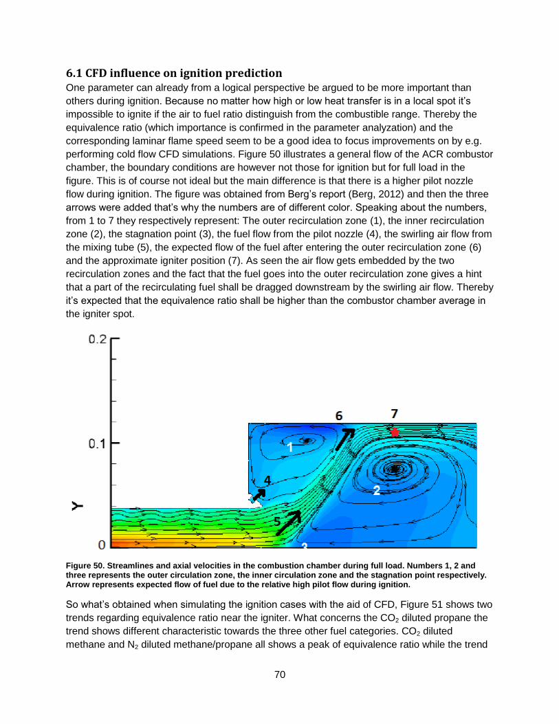
70
6.1 CFD influence on ignition prediction One parameter can already from a logical perspective be argued to be more important than
others during ignition. Because no matter how high or low heat transfer is in a local spot it’s
impossible to ignite if the air to fuel ratio distinguish from the combustible range. Thereby the
equivalence ratio (which importance is confirmed in the parameter analyzation) and the
corresponding laminar flame speed seem to be a good idea to focus improvements on by e.g.
performing cold flow CFD simulations. Figure 50 illustrates a general flow of the ACR combustor
chamber, the boundary conditions are however not those for ignition but for full load in the
figure. This is of course not ideal but the main difference is that there is a higher pilot nozzle
flow during ignition. The figure was obtained from Berg’s report (Berg, 2012) and then the three
arrows were added that’s why the numbers are of different color. Speaking about the numbers,
from 1 to 7 they respectively represent: The outer recirculation zone (1), the inner recirculation
zone (2), the stagnation point (3), the fuel flow from the pilot nozzle (4), the swirling air flow from
the mixing tube (5), the expected flow of the fuel after entering the outer recirculation zone (6)
and the approximate igniter position (7). As seen the air flow gets embedded by the two
recirculation zones and the fact that the fuel goes into the outer recirculation zone gives a hint
that a part of the recirculating fuel shall be dragged downstream by the swirling air flow. Thereby
it’s expected that the equivalence ratio shall be higher than the combustor chamber average in
the igniter spot.
Figure 50. Streamlines and axial velocities in the combustion chamber during full load. Numbers 1, 2 and three represents the outer circulation zone, the inner circulation zone and the stagnation point respectively. Arrow represents expected flow of fuel due to the relative high pilot flow during ignition.
So what’s obtained when simulating the ignition cases with the aid of CFD, Figure 51 shows two
trends regarding equivalence ratio near the igniter. What concerns the CO2 diluted propane the
trend shows different characteristic towards the three other fuel categories. CO2 diluted
methane and N2 diluted methane/propane all shows a peak of equivalence ratio while the trend

71
for CO2 diluted propane shows a steadily increasing equivalence ratio for increased amount of
CO2. What is to be noticed from Figure 51 is that the equivalence ratio around the ignition point
for pure methane and propane is below combustor chamber average that has been shown not
to predict any ignition at all. This does not seem realistic since indeed pure methane and
propane is shown to ignite just perfectly according to Berg (Berg, 2012) among others. So
maybe it’s questionable if the 2-equation SST turbulence model is capable of predicting the
mixing obtained from turbulence.
The trend for the three smaller ignition volumes is equal to the 10 mm radius sphere and only
shows a translation in the vertical direction compared to what’s displayed in Figure 51. For
absolute values and data for the three smaller ignition volumes the reader is referred to the
appendix.
Figure 51. CFD average equivalence ratio for the 10 mm ignition sphere and the combustor chamber as a function of the amount inert gases.
As displayed by Figure 52 the laminar flame speed trend are similar to the equivalence ratio
trend for the ignition volumes. However the displayed correlations to the amount of inert gas is
slightly more aggressive due to the polynomial relation between the equivalence ratio and the
laminar flame speed, see Figure 22. Also Figure 52 can be used to state the question if the
turbulence model is accurate enough since the laminar flame speed, that is directly connected
to the Karlovitz number and directly correlated to the equivalence ratio, is predicted lower than
the CC average for the pure hydrocarbons.
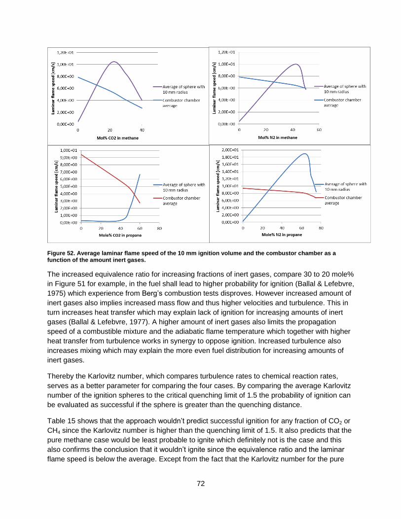
72
Figure 52. Average laminar flame speed of the 10 mm ignition volume and the combustor chamber as a function of the amount inert gases.
The increased equivalence ratio for increasing fractions of inert gases, compare 30 to 20 mole%
in Figure 51 for example, in the fuel shall lead to higher probability for ignition (Ballal & Lefebvre,
1975) which experience from Berg’s combustion tests disproves. However increased amount of
inert gases also implies increased mass flow and thus higher velocities and turbulence. This in
turn increases heat transfer which may explain lack of ignition for increasing amounts of inert
gases (Ballal & Lefebvre, 1977). A higher amount of inert gases also limits the propagation
speed of a combustible mixture and the adiabatic flame temperature which together with higher
heat transfer from turbulence works in synergy to oppose ignition. Increased turbulence also
increases mixing which may explain the more even fuel distribution for increasing amounts of
inert gases.
Thereby the Karlovitz number, which compares turbulence rates to chemical reaction rates,
serves as a better parameter for comparing the four cases. By comparing the average Karlovitz
number of the ignition spheres to the critical quenching limit of 1.5 the probability of ignition can
be evaluated as successful if the sphere is greater than the quenching distance.
Table 15 shows that the approach wouldn’t predict successful ignition for any fraction of CO2 or
CH4 since the Karlovitz number is higher than the quenching limit of 1.5. It also predicts that the
pure methane case would be least probable to ignite which definitely not is the case and this
also confirms the conclusion that it wouldn’t ignite since the equivalence ratio and the laminar
flame speed is below the average. Except from the fact that the Karlovitz number for the pure
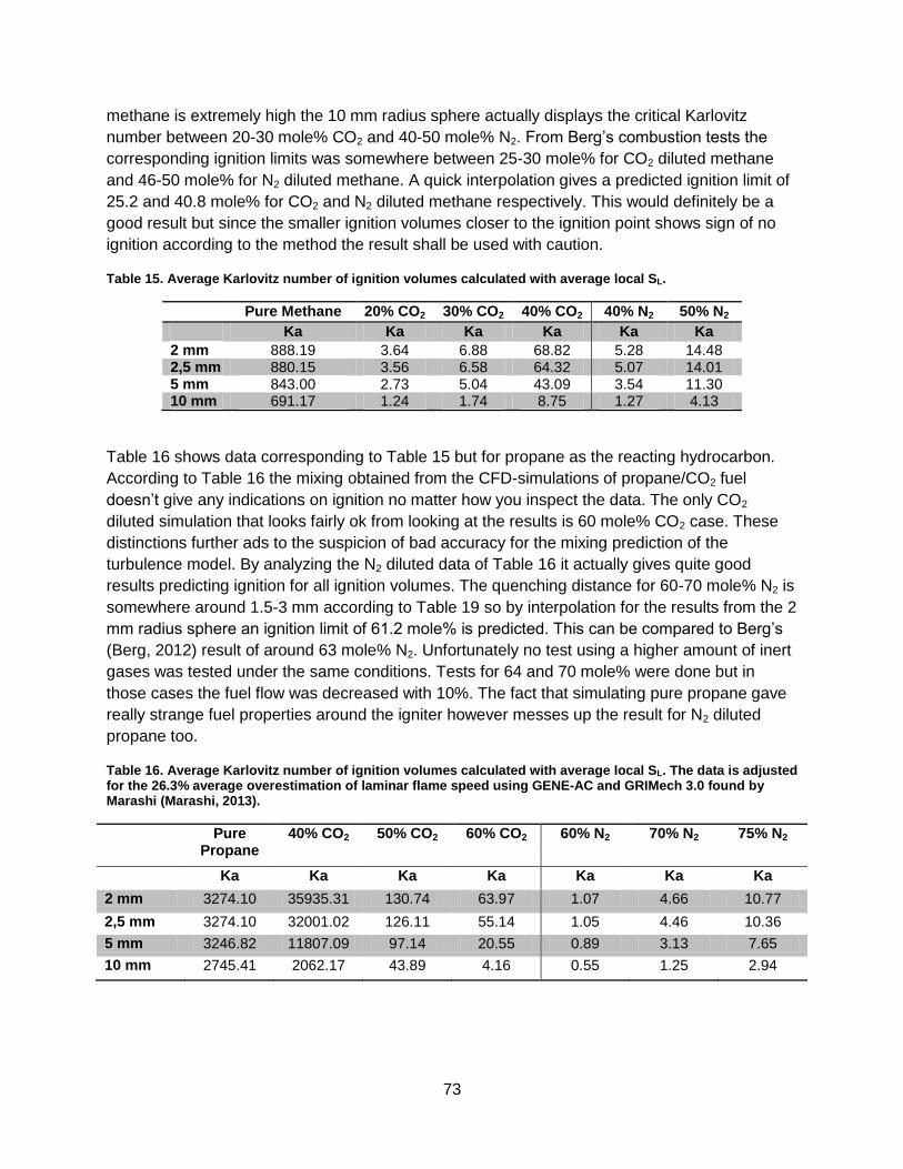
73
methane is extremely high the 10 mm radius sphere actually displays the critical Karlovitz
number between 20-30 mole% CO2 and 40-50 mole% N2. From Berg’s combustion tests the
corresponding ignition limits was somewhere between 25-30 mole% for CO2 diluted methane
and 46-50 mole% for N2 diluted methane. A quick interpolation gives a predicted ignition limit of
25.2 and 40.8 mole% for CO2 and N2 diluted methane respectively. This would definitely be a
good result but since the smaller ignition volumes closer to the ignition point shows sign of no
ignition according to the method the result shall be used with caution.
Table 15. Average Karlovitz number of ignition volumes calculated with average local SL.
Pure Methane 20% CO2 30% CO2 40% CO2 40% N2 50% N2
Ka Ka Ka Ka Ka Ka
2 mm 888.19 3.64 6.88 68.82 5.28 14.48 2,5 mm 880.15 3.56 6.58 64.32 5.07 14.01 5 mm 843.00 2.73 5.04 43.09 3.54 11.30 10 mm 691.17 1.24 1.74 8.75 1.27 4.13
Table 16 shows data corresponding to Table 15 but for propane as the reacting hydrocarbon.
According to Table 16 the mixing obtained from the CFD-simulations of propane/CO2 fuel
doesn’t give any indications on ignition no matter how you inspect the data. The only CO2
diluted simulation that looks fairly ok from looking at the results is 60 mole% CO2 case. These
distinctions further ads to the suspicion of bad accuracy for the mixing prediction of the
turbulence model. By analyzing the N2 diluted data of Table 16 it actually gives quite good
results predicting ignition for all ignition volumes. The quenching distance for 60-70 mole% N2 is
somewhere around 1.5-3 mm according to Table 19 so by interpolation for the results from the 2
mm radius sphere an ignition limit of 61.2 mole% is predicted. This can be compared to Berg’s
(Berg, 2012) result of around 63 mole% N2. Unfortunately no test using a higher amount of inert
gases was tested under the same conditions. Tests for 64 and 70 mole% were done but in
those cases the fuel flow was decreased with 10%. The fact that simulating pure propane gave
really strange fuel properties around the igniter however messes up the result for N2 diluted
propane too.
Table 16. Average Karlovitz number of ignition volumes calculated with average local SL. The data is adjusted for the 26.3% average overestimation of laminar flame speed using GENE-AC and GRIMech 3.0 found by Marashi (Marashi, 2013).
Pure Propane
40% CO2 50% CO2 60% CO2 60% N2 70% N2 75% N2
Ka Ka Ka Ka Ka Ka Ka
2 mm 3274.10 35935.31 130.74 63.97 1.07 4.66 10.77
2,5 mm 3274.10 32001.02 126.11 55.14 1.05 4.46 10.36
5 mm 3246.82 11807.09 97.14 20.55 0.89 3.13 7.65
10 mm 2745.41 2062.17 43.89 4.16 0.55 1.25 2.94

74
In Figure 53 Berg’s results according to Figure 3 is re-created together with the ignition limits
predicted from the CFD-simulations and the 10 mm radius ignition volume. In some sense the
prediction is fairly good for all fuel groups except the CO2 diluted propane but the results also
displays that the ignition probability shall increase with the amount inert gases and then
decrease again. The reason that the two ignition limits from the CFD result for nitrogen diluted
methane is almost identical was because no fuel composition between pure propane and the 40
mole% N2 was made. Thereby the “No ignition CFD (10 mm) limit was interpolated towards the
pure propane result which makes the two limits appear as almost identical, see Table 15 for
data.
Figure 53. Predicted ignition limits from CFD results from the 10 mm ignition sphere which is compared to experimental limits for propane and methane. No prediction was possible for CO2 diluted propane.
Besides Table 15 figures like Figure 54 is helpful to get a full scale impression of the ignition
possibilities according to the Karlovitz number. The red volumes seen represent the areas
where the Karlovitz number is below the ignitable limit of 1.5 presented by Abdel-Gayed and
Bradley (Abdel-Gayed & Bradley, 1985). The method behind obtaining the figure is though
subject to some error of fitting a regression line to the correlation between the laminar flame
speed and the equivalence ratio. The errors shall however be relatively small and similar for
each case. In Figure 54 CO2 diluted methane is presented and if the reader is interested in
similar figures for the rest of the fuel groups these can be found in the appendix.
It’s not super clear but for all cases diluted by CO2, Figure 54, the ignitable cloud reaches or at
least stretches very close to the ignition point somewhere up to the ignition limit obtained by
Berg (Berg, 2012). The ignition limit for methane/CO2 was somewhere between 25-30 mole%
i.e. the between the top right and the bottom left illustration of Figure 54. What’s strange, though
0
20
40
60
80
100
120
140
0% 20% 40% 60% 80%
MIE
incr
eas
e in
%
Mole% inert gases in fuel
CO2 methane
N2 methane
CO2 propane
N2 propane
Ignition (Berg)
No ignition (Berg)
Ignition limit CFD (10 mm)
No ignition CFD (10 mm)

75
consistent with the result of Table 15, is the result that the area around the igniter is not near
ignitable for the pure methane case which certainly not is comparable to the reality.
Figure 54. Volume of the combustor chamber displaying all cells with a Karlovitz number below 1.5 when local equivalence ratio is used. The amount CO2 increases from 0 to 40 mole% in a z-pattern.
So this far the method has shown some possibility to predict ignition but the results aren’t
straightforward and it’s questionable if the utilized turbulence model is accurate enough when it
comes to predicting the mixing of air and fuel near the igniter. To get a grip on how much off the
mixing is and also to give a feeling on which air to fuel ratio to be expected for each fuel
composition approximated minimum equivalence ratios and laminar flame speeds for predicted
ignition could be calculated. By assuming that the RMS velocity and the kinematic viscosity is
constant at their global average for all fuel cases then an approximate laminar flame speed for
obtaining a Karlovitz number of 1.5 and thus predicted ignition can be approximated.
Equivalence ratios for each fuel composition can then be obtained from the correlation towards
the laminar flame speed for a specific fuel composition.
Figure 55 gives the trend of minimum equivalence ratio for obtaining ignition when the fraction
of inert gases is increased. The green circle and the red rectangle respectively represent the
minimum equivalence ratio for matching Berg’s ignition and no ignition limit. From Figure 55 it

76
can be verified that the combustor chamber average indeed is below the properties for ignition
at all fractions of inert gases. The CFD results can also be verified to be relatively good at
catching the ignition interval found by Berg (Berg, 2012). Figure 55 further strengthens the idea
of bad mixing accuracy of the turbulence model and in general it seems to under predict the
concentration of hydrocarbons.
Figure 55. Average equivalence ratio of combustor chamber and 10 mm ignition sphere compared to estimated minimum equivalence ratio to predict ignition.
Table 17 displays the expected equivalence ratio around the igniter for prediction within Berg’s
limits for each fuel group. It tells something about what could be expected if performing
experimental tests on mixing in the future.
Table 17. Approximated equivalence ratio expected around igniter spot.
Equivalence ratio at ignition limit
Methane/CO2 Methane/N2 Propane/CO2 Propane/N2
Ignition (Berg) 0.668 0.642 0.617 0.585
No ignition (Berg) 0.679 0.648 0.633 0.593
The minimum laminar flame speed that corresponds to the minimum equivalence ratio in Figure
55 is presented in Figure 56. The reason that the minimum laminar flame speed is constant as a
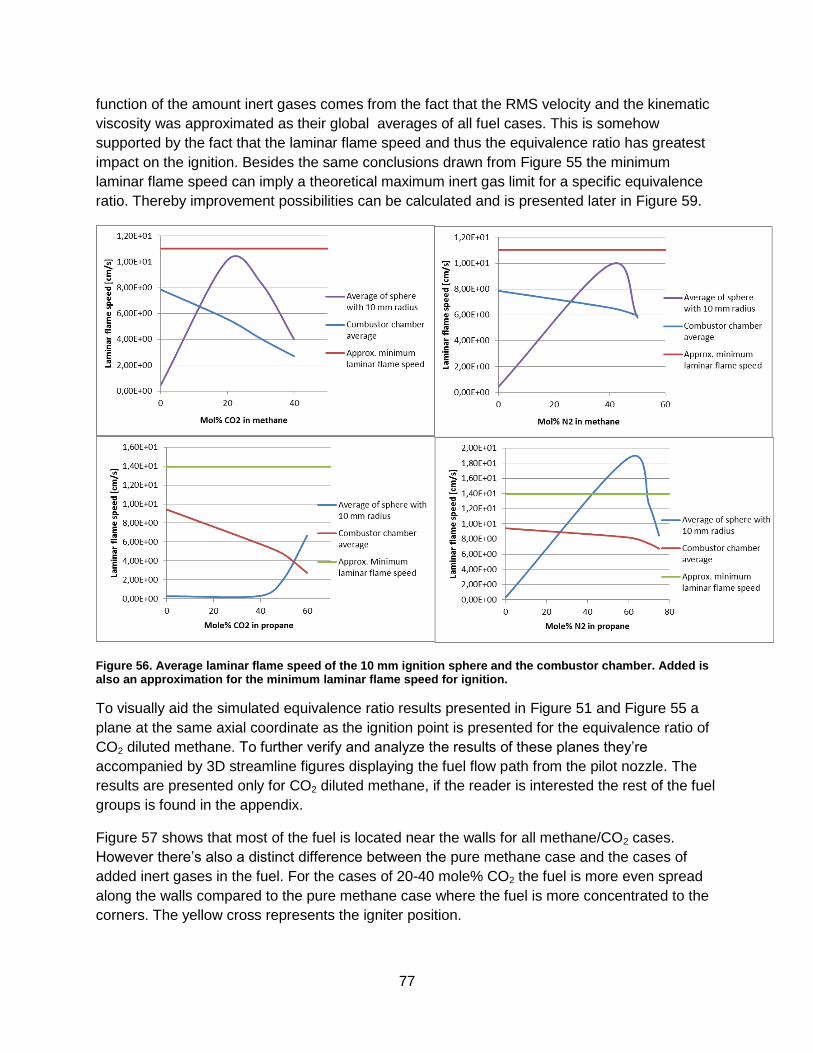
77
function of the amount inert gases comes from the fact that the RMS velocity and the kinematic
viscosity was approximated as their global averages of all fuel cases. This is somehow
supported by the fact that the laminar flame speed and thus the equivalence ratio has greatest
impact on the ignition. Besides the same conclusions drawn from Figure 55 the minimum
laminar flame speed can imply a theoretical maximum inert gas limit for a specific equivalence
ratio. Thereby improvement possibilities can be calculated and is presented later in Figure 59.
Figure 56. Average laminar flame speed of the 10 mm ignition sphere and the combustor chamber. Added is also an approximation for the minimum laminar flame speed for ignition.
To visually aid the simulated equivalence ratio results presented in Figure 51 and Figure 55 a
plane at the same axial coordinate as the ignition point is presented for the equivalence ratio of
CO2 diluted methane. To further verify and analyze the results of these planes they’re
accompanied by 3D streamline figures displaying the fuel flow path from the pilot nozzle. The
results are presented only for CO2 diluted methane, if the reader is interested the rest of the fuel
groups is found in the appendix.
Figure 57 shows that most of the fuel is located near the walls for all methane/CO2 cases.
However there’s also a distinct difference between the pure methane case and the cases of
added inert gases in the fuel. For the cases of 20-40 mole% CO2 the fuel is more even spread
along the walls compared to the pure methane case where the fuel is more concentrated to the
corners. The yellow cross represents the igniter position.

78
Figure 57. Time averaged equivalence ratio profiles on the plane of the ignition point, normal to the axial direction and with current view facing the burner. Mole% of CO2 in the methane based fuel increases in a Z-pattern.
This fuel distribution from the CFD simulations can be verified by viewing streamlines from the
pilot fuel nozzle, Figure 58 illustrates fuel stream lines together with the equivalence ratio plane
presented in Figure 57.
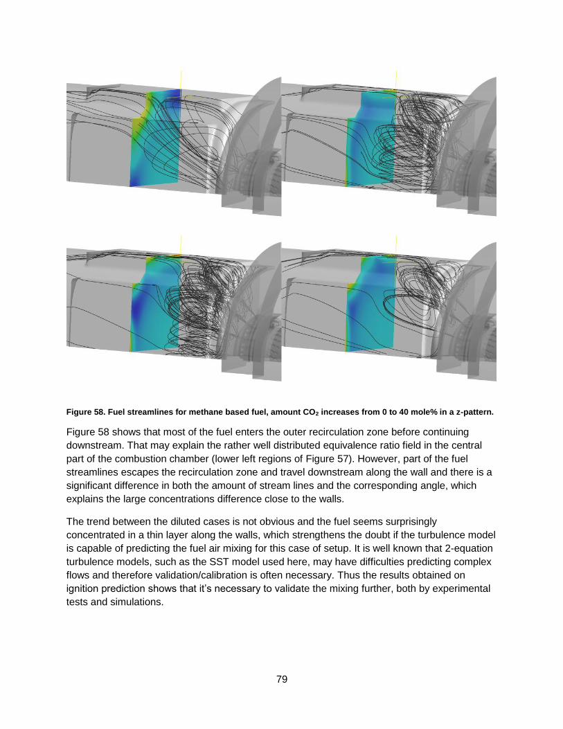
79
Figure 58. Fuel streamlines for methane based fuel, amount CO2 increases from 0 to 40 mole% in a z-pattern.
Figure 58 shows that most of the fuel enters the outer recirculation zone before continuing
downstream. That may explain the rather well distributed equivalence ratio field in the central
part of the combustion chamber (lower left regions of Figure 57). However, part of the fuel
streamlines escapes the recirculation zone and travel downstream along the wall and there is a
significant difference in both the amount of stream lines and the corresponding angle, which
explains the large concentrations difference close to the walls.
The trend between the diluted cases is not obvious and the fuel seems surprisingly
concentrated in a thin layer along the walls, which strengthens the doubt if the turbulence model
is capable of predicting the fuel air mixing for this case of setup. It is well known that 2-equation
turbulence models, such as the SST model used here, may have difficulties predicting complex
flows and therefore validation/calibration is often necessary. Thus the results obtained on
ignition prediction shows that it’s necessary to validate the mixing further, both by experimental
tests and simulations.
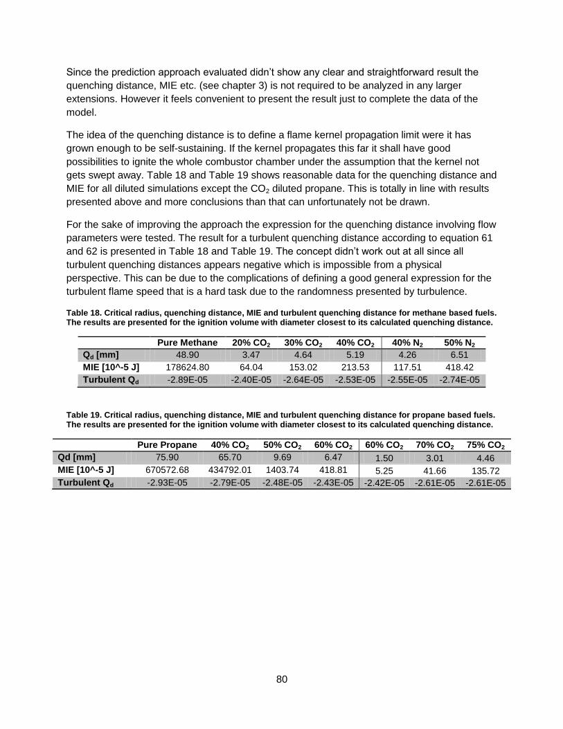
80
Since the prediction approach evaluated didn’t show any clear and straightforward result the
quenching distance, MIE etc. (see chapter 3) is not required to be analyzed in any larger
extensions. However it feels convenient to present the result just to complete the data of the
model.
The idea of the quenching distance is to define a flame kernel propagation limit were it has
grown enough to be self-sustaining. If the kernel propagates this far it shall have good
possibilities to ignite the whole combustor chamber under the assumption that the kernel not
gets swept away. Table 18 and Table 19 shows reasonable data for the quenching distance and
MIE for all diluted simulations except the CO2 diluted propane. This is totally in line with results
presented above and more conclusions than that can unfortunately not be drawn.
For the sake of improving the approach the expression for the quenching distance involving flow
parameters were tested. The result for a turbulent quenching distance according to equation 61
and 62 is presented in Table 18 and Table 19. The concept didn’t work out at all since all
turbulent quenching distances appears negative which is impossible from a physical
perspective. This can be due to the complications of defining a good general expression for the
turbulent flame speed that is a hard task due to the randomness presented by turbulence.
Table 18. Critical radius, quenching distance, MIE and turbulent quenching distance for methane based fuels. The results are presented for the ignition volume with diameter closest to its calculated quenching distance.
Pure Methane 20% CO2 30% CO2 40% CO2 40% N2 50% N2
Qd [mm] 48.90 3.47 4.64 5.19 4.26 6.51
MIE [10^-5 J] 178624.80 64.04 153.02 213.53 117.51 418.42
Turbulent Qd -2.89E-05 -2.40E-05 -2.64E-05 -2.53E-05 -2.55E-05 -2.74E-05
Table 19. Critical radius, quenching distance, MIE and turbulent quenching distance for propane based fuels. The results are presented for the ignition volume with diameter closest to its calculated quenching distance.
Pure Propane 40% CO2 50% CO2 60% CO2 60% CO2 70% CO2 75% CO2
Qd [mm] 75.90 65.70 9.69 6.47 1.50 3.01 4.46
MIE [10^-5 J] 670572.68 434792.01 1403.74 418.81 5.25 41.66 135.72
Turbulent Qd -2.93E-05 -2.79E-05 -2.48E-05 -2.43E-05 -2.42E-05 -2.61E-05 -2.61E-05
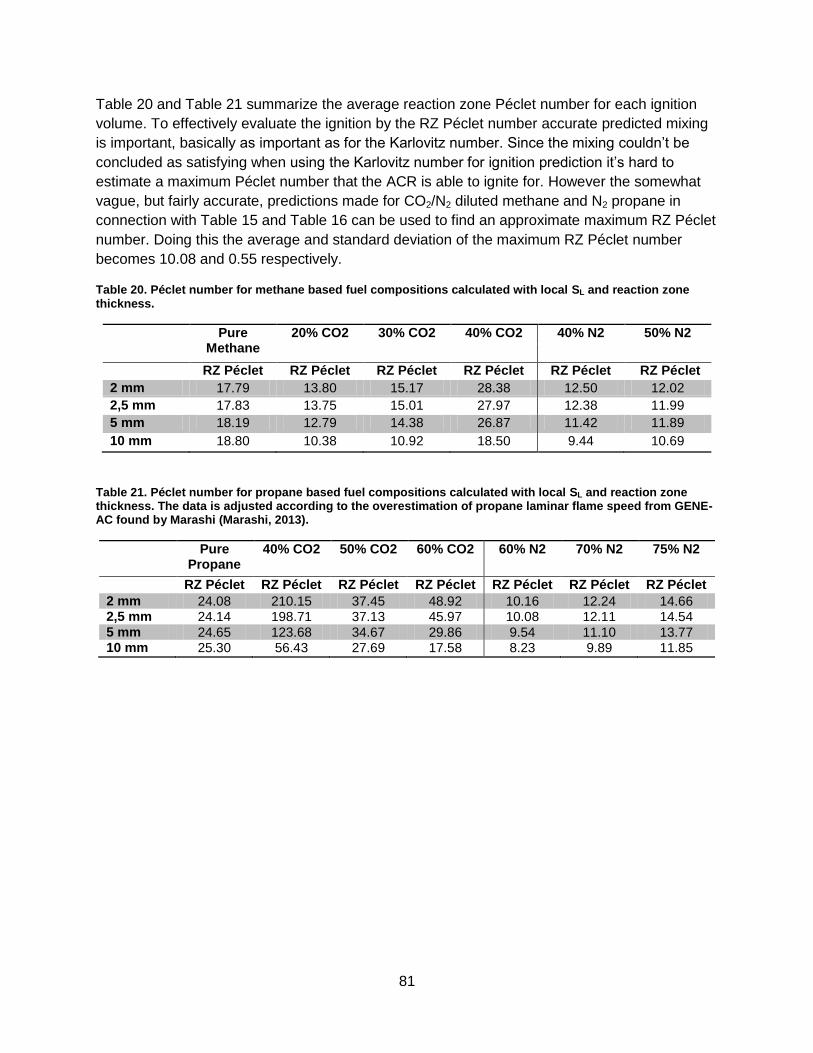
81
Table 20 and Table 21 summarize the average reaction zone Péclet number for each ignition
volume. To effectively evaluate the ignition by the RZ Péclet number accurate predicted mixing
is important, basically as important as for the Karlovitz number. Since the mixing couldn’t be
concluded as satisfying when using the Karlovitz number for ignition prediction it’s hard to
estimate a maximum Péclet number that the ACR is able to ignite for. However the somewhat
vague, but fairly accurate, predictions made for CO2/N2 diluted methane and N2 propane in
connection with Table 15 and Table 16 can be used to find an approximate maximum RZ Péclet
number. Doing this the average and standard deviation of the maximum RZ Péclet number
becomes 10.08 and 0.55 respectively.
Table 20. Péclet number for methane based fuel compositions calculated with local SL and reaction zone thickness.
Pure Methane
20% CO2 30% CO2 40% CO2 40% N2 50% N2
RZ Péclet RZ Péclet RZ Péclet RZ Péclet RZ Péclet RZ Péclet
2 mm 17.79 13.80 15.17 28.38 12.50 12.02
2,5 mm 17.83 13.75 15.01 27.97 12.38 11.99
5 mm 18.19 12.79 14.38 26.87 11.42 11.89
10 mm 18.80 10.38 10.92 18.50 9.44 10.69
Table 21. Péclet number for propane based fuel compositions calculated with local SL and reaction zone thickness. The data is adjusted according to the overestimation of propane laminar flame speed from GENE-AC found by Marashi (Marashi, 2013).
Pure Propane
40% CO2 50% CO2 60% CO2 60% N2 70% N2 75% N2
RZ Péclet RZ Péclet RZ Péclet RZ Péclet RZ Péclet RZ Péclet RZ Péclet
2 mm 24.08 210.15 37.45 48.92 10.16 12.24 14.66 2,5 mm 24.14 198.71 37.13 45.97 10.08 12.11 14.54 5 mm 24.65 123.68 34.67 29.86 9.54 11.10 13.77 10 mm 25.30 56.43 27.69 17.58 8.23 9.89 11.85
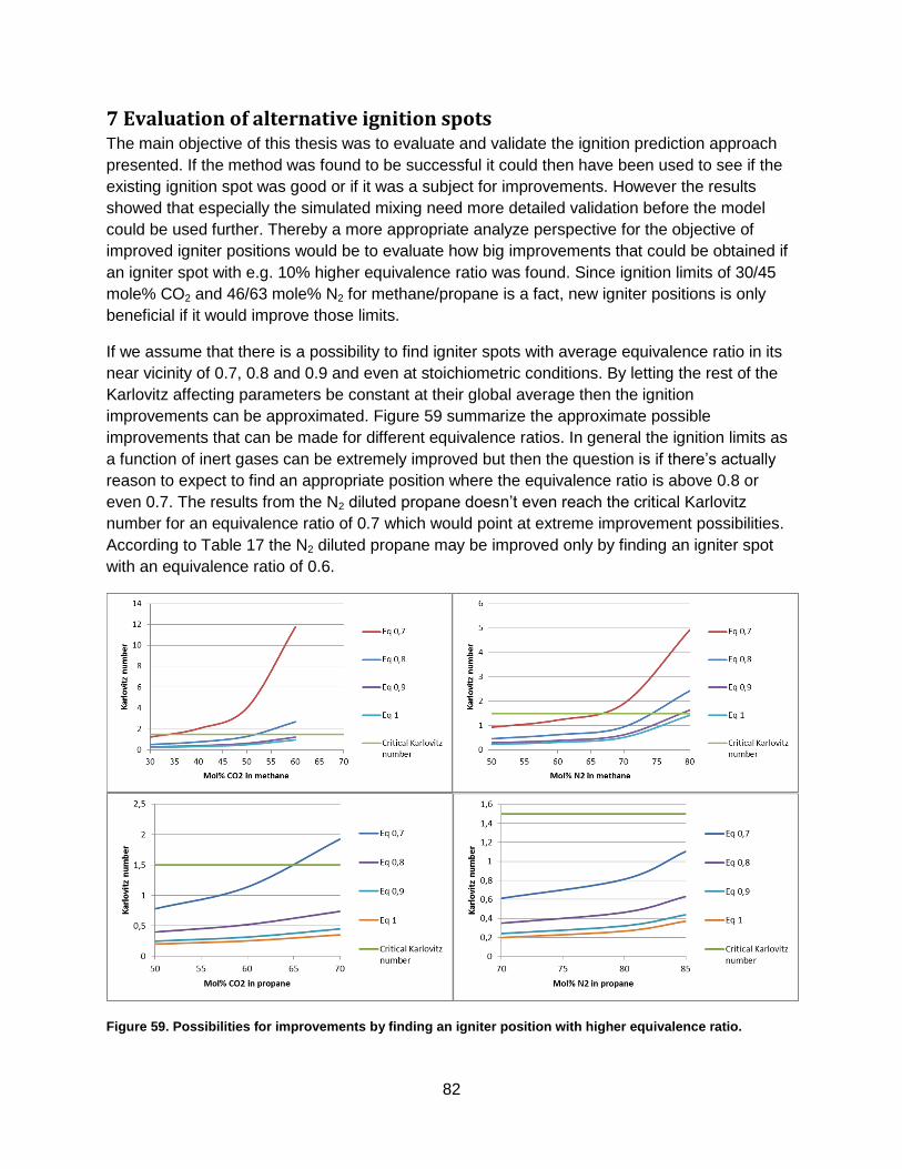
82
7 Evaluation of alternative ignition spots The main objective of this thesis was to evaluate and validate the ignition prediction approach
presented. If the method was found to be successful it could then have been used to see if the
existing ignition spot was good or if it was a subject for improvements. However the results
showed that especially the simulated mixing need more detailed validation before the model
could be used further. Thereby a more appropriate analyze perspective for the objective of
improved igniter positions would be to evaluate how big improvements that could be obtained if
an igniter spot with e.g. 10% higher equivalence ratio was found. Since ignition limits of 30/45
mole% CO2 and 46/63 mole% N2 for methane/propane is a fact, new igniter positions is only
beneficial if it would improve those limits.
If we assume that there is a possibility to find igniter spots with average equivalence ratio in its
near vicinity of 0.7, 0.8 and 0.9 and even at stoichiometric conditions. By letting the rest of the
Karlovitz affecting parameters be constant at their global average then the ignition
improvements can be approximated. Figure 59 summarize the approximate possible
improvements that can be made for different equivalence ratios. In general the ignition limits as
a function of inert gases can be extremely improved but then the question is if there’s actually
reason to expect to find an appropriate position where the equivalence ratio is above 0.8 or
even 0.7. The results from the N2 diluted propane doesn’t even reach the critical Karlovitz
number for an equivalence ratio of 0.7 which would point at extreme improvement possibilities.
According to Table 17 the N2 diluted propane may be improved only by finding an igniter spot
with an equivalence ratio of 0.6.
Figure 59. Possibilities for improvements by finding an igniter position with higher equivalence ratio.

83
The increased amount of inert gases possible to ignite for at an equivalence ratio of 0.7 is
presented in Table 22.
Table 22. Comparison of experimental ignition limits to predicted improvements for an equivalence ratio of 0.7.
Methane/CO2 Methane/N2 Propane/CO2 Propane/N2
Present limit 25-30 mole% 46-50 mole% 45-50 mole% ~63 mole%
Eq 0.7 ~35mole% ~67.5 mole% ~65 mole% >80 mole%
According to Table 22 good improvements on ignition performance may be obtained if igniter
positions with just slightly higher equivalence ratio than the values approximated in Table 17. If
future works confirms that the predicted mixing is the problem and not the expression and
Karlovitz limit itself a similar approach to the one presented below can be implemented to
evaluate better igniter positions. The approach for finding improved igniter positions presented
in chapter 7.1 is made for the present data of the CO2 diluted methane case. It also shows that
using the present mixing an improved igniter spot can’t be found.
7.1 Methane/CO2 Just by comparing the four fuel compositions on the basis of Figure 60 the equivalence ratio can
be seen as relatively homogeneous downstream the outer recirculation zone (see the most fuel
concentrated space to the left of the ignition volumes). The only exception is the pure methane
case where the fuel concentration increases significantly in the north direction of the current
ignition point. This shows that the trend seen for pure methane in Figure 57 and Figure 65 goes
for planes even downstream the current ignition position.
Figure 60. Equivalence ratio along the combustor chamber at the same height as the ignition point, the black spot. 21 ignition volumes with radius 5 mm is added to evaluate ignition probability towards the 5 mm ignition volume around present ignition point.
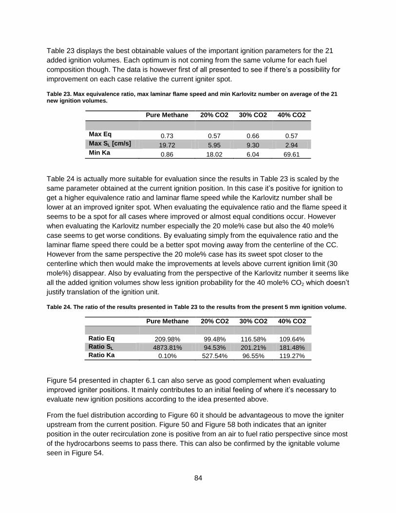
84
Table 23 displays the best obtainable values of the important ignition parameters for the 21
added ignition volumes. Each optimum is not coming from the same volume for each fuel
composition though. The data is however first of all presented to see if there’s a possibility for
improvement on each case relative the current igniter spot.
Table 23. Max equivalence ratio, max laminar flame speed and min Karlovitz number on average of the 21 new ignition volumes.
Pure Methane 20% CO2 30% CO2 40% CO2
Max Eq 0.73 0.57 0.66 0.57 Max SL [cm/s] 19.72 5.95 9.30 2.94 Min Ka 0.86 18.02 6.04 69.61
Table 24 is actually more suitable for evaluation since the results in Table 23 is scaled by the
same parameter obtained at the current ignition position. In this case it’s positive for ignition to
get a higher equivalence ratio and laminar flame speed while the Karlovitz number shall be
lower at an improved igniter spot. When evaluating the equivalence ratio and the flame speed it
seems to be a spot for all cases where improved or almost equal conditions occur. However
when evaluating the Karlovitz number especially the 20 mole% case but also the 40 mole%
case seems to get worse conditions. By evaluating simply from the equivalence ratio and the
laminar flame speed there could be a better spot moving away from the centerline of the CC.
However from the same perspective the 20 mole% case has its sweet spot closer to the
centerline which then would make the improvements at levels above current ignition limit (30
mole%) disappear. Also by evaluating from the perspective of the Karlovitz number it seems like
all the added ignition volumes show less ignition probability for the 40 mole% CO2 which doesn’t
justify translation of the ignition unit.
Table 24. The ratio of the results presented in Table 23 to the results from the present 5 mm ignition volume.
Pure Methane 20% CO2 30% CO2 40% CO2
Ratio Eq 209.98% 99.48% 116.58% 109.64% Ratio SL 4873.81% 94.53% 201.21% 181.48% Ratio Ka 0.10% 527.54% 96.55% 119.27%
Figure 54 presented in chapter 6.1 can also serve as good complement when evaluating
improved igniter positions. It mainly contributes to an initial feeling of where it’s necessary to
evaluate new ignition positions according to the idea presented above.
From the fuel distribution according to Figure 60 it should be advantageous to move the igniter
upstream from the current position. Figure 50 and Figure 58 both indicates that an igniter
position in the outer recirculation zone is positive from an air to fuel ratio perspective since most
of the hydrocarbons seems to pass there. This can also be confirmed by the ignitable volume
seen in Figure 54.

85
8 Discussion Using the results from utilizing CFD and the 10 mm ignition volume showed fairly good ignition
prediction at least when comparing to Berg’s limits of ignition. This fact gives some hopeful
expectations that the approach could give satisfying and reliable results after it has been
validated further.
The results for prediction was however not straightforward and the ignition trend showed that
ignition could be improved by adding inert gases. The main conclusion drawn from the
prediction was that the SST turbulence model probably didn’t manage to predict the mixing
accurate enough. This then gave great impact on the prediction since the equivalence ratio and
the corresponding laminar flame speed had great influence on the Karlovitz number that was
used for finding the limits of ignition.
Using the assumption of a perfectly mixed combustion chamber also showed some possibility to
predict the experimental ignition limits obtained by Berg (Berg, 2012). However to find this
property of the even simpler model the critical Karlovitz number needed to be scaled and thus 2
of the experimental ignition limits was used for the scaling purpose and thereby could only 2 be
used for validation. This small amount of data to evaluate if an up scaled Karlovitz limit could be
used to get a quick intuition of ignition performance is a bit little and don’t bring too much
confidence to the perfectly mixed approach. Though if it with further validation would show that
it’s only a certain percentage from the predicted result using CFD it would be an extremely cost
effective first step of ignition prediction. The results and the discussion around them shall
however not be taken as some kind of fact and since no study has shown that the critical
Karlovitz number shall be up-scaled as a function of inert gases for now it serves only as a
interesting fact.
As stated in the results Shy et al. (Shy, et al., 2000) actually has showed changing critical
Karlovitz numbers as a function of inert gases in the fuel. These results can be seen at the end
of chapter 3.3 and according to them the limit shall decrease for increased fractions of inert
gases. The 10 mm ignition sphere results, discussed above, however related fairly well to the
critical Karlovitz number of 1.5 according to Abdel-Gayed and Bradley (Abdel-Gayed & Bradley,
1985). Moreover no other studies using this prediction approach has used anything other than
the 1.5 limit (Neophytou, et al., 2012) (Soworka, et al., 2014). These studies didn’t predict
ignition from the perspective of inert gases though but since the data presented by Shy et al.
(Shy, et al., 2000) also were somewhat poor when it comes to both fuel compositions and
equivalence ratios the 1.5 limit was decided as most appropriate. The 1.5 limit was obtained
from premixed combustion data for lean/rich methane and propane.
The fact that the 10 mm radius sphere shows ignition possibilities but not the smaller volumes
may come from the fact that the vertical coordinate, seen from the combustor wall, was not
100% clear. I was given an approximate distance of 5-10 mm from the wall and I chose 10 mm
to get at larger range of quenching distances possible to evaluate for. Since I choose to define
the igniter position 10 mm from the wall this may have influenced the prediction. Because after
all as big ignition volumes as 10 mm radius is not necessary for the sake of matching the
quenching distance. If the igniters vertical coordinate would have been set to 5 mm from the
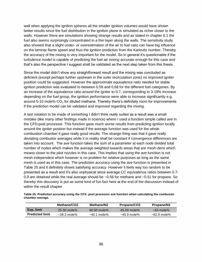
86
wall when applying the ignition spheres all the smaller ignition volumes would have shown
better results since the fuel distribution in the ignition plane is simulated as richer closer to the
walls. However there are simulations showing strange results and as stated in chapter 6.1 the
fuel also seems surprisingly concentrated in a thin layer along the walls. The sensitivity study
also showed that a slight under- or overestimation of the air to fuel ratio can have big influence
on the laminar flame speed and thus the ignition prediction from the Karlovitz number. Thereby
the accuracy of the mixing is very important for the model. So in general it’s questionable if the
turbulence model is capable of predicting the fuel air mixing accurate enough for this case and
that’s also the perspective I suggest shall be validated as the next step taken from this thesis.
Since the model didn’t show any straightforward result and the mixing was concluded as
deficient (except perhaps further upstream in the outer recirculation zone) no improved igniter
position could be suggested. However the approximate equivalence ratio needed for stable
ignition prediction was evaluated to between 0.59 and 0.68 for the different fuel categories. By
an increase of the equivalence ratio around the igniter to 0.7, corresponding to 3-19% increase
depending on the fuel group, the ignition performance were able to increase significantly e.g.
around 5-10 mole% CO2 for diluted methane. Thereby there’s definitely room for improvements
if the prediction model can be validated and improved regarding the mixing.
A last notation to be made of something I didn’t think really suited as a result was a small
mistake (like many other findings made in science) where I used a function simple called ave in
the CFD-post processor. This function gave much worse results from predicting ignition locally
around the igniter position but instead if the average function was used for the whole
combustion chamber it gave really good results. The strange thing was that it gave really
deviating combustor averages while it in reality shall be constant if convergence differences are
taken into account. The ave function takes the sum of a parameter at each node divided total
number of nodes which makes the average weighted towards areas that are mesh-dens which
means closer to the pilot nozzles in this case. This implies that using the ave function is not
mesh independent which however is no problem for relative purposes as long as the same
mesh is used as in this case. The prediction accuracy using the ave function is presented in
Table 25 and it definitely shows satisfying accuracy. However it feels way too random to be
presented as a result and it’s also unphysical since average CC equivalence ratios between 0.7-
0.9 are obtained while the real average should be ~0.56 for methane and ~0.51 for propane. So
thereby this discovery is put as some kind of fun fact here at the end of the discussion instead of
within the result chapter
Table 25. Prediction accuracy using the CFX- post processor ave function when calculating the combustor chamber average.
Methane/CO2 Methane/N2 Propane/CO2 Propane/N2
Exp. limit 25-30 mole% 46-50 mole% 45-50 mole% ~63 mole%
Predicted limit ~28.3 mole% ~40.1 mole% ~45.9 mole% ~62.9 mole%

87
8.1 Conclusions Using the Karlovitz number obtained from cold flow simulations has showed some possibilities
to work as a cost effective ignition prediction method even when the limit is set by fractions of
inert gases. However the prediction of the ignition limits in the SGT-700 burner implemented in
SIT’s atmospheric combustion rig didn’t show straightforward results. The main conclusion
drawn from the somewhat straggling results was that the turbulence model probably didn’t
predict the mixing that well and thus needed further investigation.
Since the simulated mixing was deemed unsatisfying the tendencies showed for prediction of
ignition limits couldn’t be taken as fact for an accuracy measure of the model. A model not
including CFD-simulations was also tested and found to show some kind of prediction ability if
the critical Karlovitz number was up-scaled. This result however served more as an interesting
fact since the up scaled Karlovitz number couldn’t be motivated except from that it showed
some accuracy of prediction. The scaling was influenced by the inert gas used, probably due to
its effect on the laminar flame speed of a certain hydrocarbon. The scaling needed was greater
for CO2 dilution than N2 dilution but as stated the scaling was fairly constant when going from
one fuel to another (since the predicted ignition interval showed fairly good results). If this
scaling for a certain inert gas could be verified this extremely simple model, not including any
CFD-simulations, could be possible to use also for other hydrocarbons utilized as fuel. However
to make this kind of verification to this vague model more experimental data would be needed.
Due to the unreliable mixing the objective of evaluating improved igniter spots was hard to
perform. Instead possible improvements at small increases of equivalence ratios was presented
and found to be really good. After all I believe the model is possible to be implemented on one
of SIT’s present gas turbine geometries. First it needs some improvements regarding the
turbulence mixing though and in my opinion it shall be tested in the SGT-700 geometry as soon
it’s been fixed.
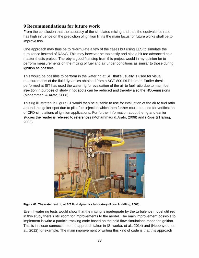
88
9 Recommendations for future work From the conclusion that the accuracy of the simulated mixing and thus the equivalence ratio
has high influence on the prediction of ignition limits the main focus for future works shall be to
improve this.
One approach may thus be to re-simulate a few of the cases but using LES to simulate the
turbulence instead of RANS. This may however be too costly and also a bit too advanced as a
master thesis project. Thereby a good first step from this project would in my opinion be to
perform measurements on the mixing of fuel and air under conditions as similar to those during
ignition as possible.
This would be possible to perform in the water rig at SIT that’s usually is used for visual
measurements of the fluid dynamics obtained from a SGT-800 DLE-burner. Earlier thesis
performed at SIT has used the water rig for evaluation of the air to fuel ratio due to main fuel
injection in purpose of study if hot spots can be reduced and thereby also the NOx-emissions
(Mohammadi & Arato, 2008).
This rig illustrated in Figure 61 would then be suitable to use for evaluation of the air to fuel ratio
around the igniter spot due to pilot fuel injection which then further could be used for verification
of CFD-simulations of ignition applications. For further information about the rig and earlier
studies the reader is referred to references (Mohammadi & Arato, 2008) and (Roos & Halling,
2008).
Figure 61. The water test rig at SIT fluid dynamics laboratory (Roos & Halling, 2008).
Even if water rig tests would show that the mixing is inadequate by the turbulence model utilized
in this study there’s still room for improvements to the model. The main improvement possible to
implement is write a particle tracking code based on the cold flow simulations made for ignition.
This is in closer connection to the approach taken in (Soworka, et al., 2014) and (Neophytou, et
al., 2012) for example. The main improvement of writing this kind of code is that this approach

89
would not need the assumption that as long the flame kernel grows above its steady state it will
propagate towards the primary zone. This type of code is probably very time-consuming to write
but as a master thesis for a computer science engineer it could serve as a good challenge. At
the same time the code would be helpful if the approach of cold flow ignition prediction in the
future is transferred to SIT’s gas turbine specific combustor geometries.
For the interest of comparing how results is affected by the CFD-software used a future work
could also be to investigate differences between CFX and Fluent. One perspective to look at
could then be to compare how the different constant settings for the SST turbulence model
affect the results. Another perspective could be to investigate discretization differences between
the two CFD codes.

90
Bibliography Abdel-Gayed, R. & Bradley, D., 1985. Criteria for Turbulent propagation Limits of Premixed
Flames. Combustion and Flame, 62(52), pp. 61-68.
Ballal, D. & Lefebvre, A., 1975. The influence of flow parameters on minimum ignition energy
and quenching distance. Symposium on Combustion, 15(1), pp. 1473-1481.
Ballal, D. & Lefebvre, A., 1977. Ignition and flame quenching in flowing gaseous mixtures.
Proceedings of the Royal Society London A, Volume 357, pp. 163-181.
Ballal, D. & Lefebvre, A., 1981. A general model of spark ignition for gaseous and liquid fuel-air
mixtures. s.l., University of Waterloo.
Barnett, H. & Hibbard, R., 1957. Basic considerations in the combustion of hydrocarbon fuels
with air., s.l.: NACA.
Berg, A., 2012. Flexible Ignition System for a Gas Turbine, Stockholm: KTH Industrial
Engineering and Management.
Borghi, R., 1985. On the structure and morphology of turbulent premixed flames. In: Recent
Advances in the Aerospace Science. New York: Plenum, pp. 117-138.
Brokaw, R. & Gerstein , m., 1957. Correlations of burning velocity, quenching distances and
minimum ignition energies for hydrocarbon-oxygen-nitrogen systems. Symposium on
Combustion, 6(1), pp. 66-74.
CFD-Online, 2011. CFD Online. [Online]
Available at: http://www.cfd-online.com/Wiki/SST_k-omega_model
[Accessed 17 June 2015].
Dahoe, A. & de Goey, L., 2003. On the determination of the laminar burning velocity from closed
vessel gas explosions. Journal of Loss Prevention in the Process Industries, Volume 16, pp.
457-478.
Gutkowski, A. N. & Parra-Santos, T., 2014. Quenching Distance and Quenching Diameter Ratio
for Flames Propagating In Propane/Air Mixtures. Prague, Lodz University of Technology,
Institute of Turbomachinery.
Hellberg, A. & Nordén, G., 2009. Siemens SGT-700 gas turbine performance yields more power
and higher efficiancy. s.l., Siemens Industrial Turbomachinery.
Heravi, H. et al., 2007. Determination of Laminar Flame Thickness and Burning Velocity of
Methane-Air Mixture. European Combustion Meeting, Chania.
Horrocs, G., 2011. CFD-Online. [Online]
Available at: http://www.cfd-online.com/Forums/cfx/86254-turbulence-modeling-cfx.html
[Accessed 31 July 2015].
91
Korén, D., 2015. Mesh study of the SGT-750 combustor - Optimization of mesh from an cost-
effective perspective, Stockholm : Royal Institute of Technology.
Lantz, A. et al., 2015. Investigation of Hydrogen Enriched Natural Gas Flames in a SGT-
700/800 Burner Using OH PLIF and Chemiluminescence Imaging. Journal of Engineering for
Gas Turbines and Power, Volume 137.
Lewis, B. & Von Elbe, G., 1987. Combustion, Flames, and Explosions of Gases. 3 ed.
s.l.:Elsevier.
Marashi, S. S., 2013. Network Modeling Application to Laminar Flame Speed and NOx
Prediction in Industrial Gas Turbines, Linkoping: Linkoping University.
Marchione, T., Ahmed, S. & Mastorakos, E., 2009. Ignition of turbulent swirling n-heptane spray
flames using single and multiple sparks.. Combustion and Flame, 156(1), pp. 166-180.
McMurtry, P., 2000. Lecture notes of course ME 7960 "Turbulence" at University of Utah.
[Online]
Available at: http://www.eng.utah.edu/~mcmurtry/Turbulence/turbulence.html
[Accessed 17 June 2015].
Mohammadi, P. & Arato, A., 2008. DLE burner water rig simulations, Mälardalen: Mälardalen
University.
Neophytou, A., 2010. Spark Ignition and Flame Propagation in Sprays, Cambridge: Uniersity of
Cambridge.
Neophytou, A., Richardson, E. & Mastorakos, E., 2012. Spark ignition of turbulent recirculating
non-premixed gas and spray flames: A model for predicting ignition probability. Combustion and
Flame, Volume 159, pp. 1503-1522.
Peters, N., 2004. Turbulent Combustion. Cambridge: Press Syndicate of the University of
Cambridge.
Qiao, L., Dahmn, W. J., Faeth, G. M. & Oran, E. S., 2008. Burning Velocitites and Flammability
Limits of Premixed Methane/Air/Diluent Flames in Microgravity. Reno, The university of
Michigan and Naval Research Laboratory, Washington.
Roos, N. & Halling, D., 2008. Experimental evaluation of the flow in a 3rd generation dry low
emissions burner, Mälardalen: Mälardalen university.
Shy, S., Lin, W. & Peng, K., 2000. Higi-Intensity Turbulent Premixed Combution: General
Correlations of Turbulent Burning Velocities In a New Cruciform Burner. Proceedings of the
Combustion Instistue, Volume 28, pp. 561-568.
Shy, S., Liu, C. & Shih, W., 2010. Ignition transition in turbulent premixed combustion.
Combustion and Flame, 157(2), pp. 341-350.
92
Siemens AB, Corporate Communications, 2013. Siemens. [Online]
Available at: http://w3.siemens.se/home/se/sv/cc/siemens-120-ar-i-
sverige/PublishingImages/120arsiemenssverige.pdf
[Accessed 3 Juni 2015].
Siemens Industrial Turbomachinery AB, 2013. Siemens. [Online]
Available at: http://www.energy.siemens.com/hq/pool/hq/power-generation/gas-
turbines/downloads/Industrial%20Gas%20Turbines/Industrial_Gas_Turbines_EN_new.pdf
[Accessed 3 Juni 2015].
SIT AB, 2012. Internal documents. s.l., s.n.
Soworka, T., Gerendas, M., Eggels, R. & Mastorakos , E., 2014. Numerical Investigation of
Ignition Performance of a Lean Burn Combustor at Sub-Atmospheric Conditions. Düsseldorf,
Rolls-Royce Deutschland together with Cambridge University.
Stone, R., Clarke, A. & Beckwith, P., 1998. Correlations for the Laminar-Burning Velocity of
Methane/Diluent/Air Mixtures Obtained in Free-Fall Experiments. Combustion and Flame,
Volume 114, pp. 545-555.
Sveriges televisions nyheter, 2011. svt. [Online]
Available at: http://www.svt.se/nyheter/regionalt/ost/finspang-siemens-i-finspang-flyttar-
angturbintillverkningen
[Accessed 03 Juni 2015].
Warnatz, J., Maas, U. & Dibble, R., 2006. Combustion: Physical and Chemical Fundamentals,
Modeling and Simulation, Experiments, Pollutant Formation. 4th ed. Berlin: Springer.
Wendt, J., 2009. Computational Fluid Dynamics An Introduction. s.l.:Springer.
Yang, S. & Shy, S., 2002. Global Quenching of Premixed CH4/Air Flames: Effects of Turbulent
Straining, Equivalence Ratio and Radiative Heat Loss. Proceedings of the Combustion Institute,
Volume 29, pp. 1841-1847.
Zhou, B., 2015. Advanced Laser-based Multi-scalar Imaging for Flame Structure Visualization
towards a Deepened Understanding of Premixed Turbulent Combustion. Lund: Lund University.

93
Appendix
Table 26. Equivalence ratio and laminar flame speed for four cases of fuel compositions varying from pure methane to methane and 40 mole% CO2.
Pure Methane 20% CO2 30% CO2 40% CO2
EquiRatio SL [cm/s] EquiRatio SL [cm/s] EquiRatio SL [cm/s] EquiRatio SL [cm/s]
2 mm 3,44E-01 3,95E-01 5,72E-01 6,10E+00 5,65E-01 4,43E+00 5,12E-01 1,50E+00
2,5 mm 3,44E-01 3,96E-01 5,74E-01 6,18E+00 5,67E-01 4,53E+00 5,14E-01 1,55E+00
5 mm 3,46E-01 4,05E-01 5,87E-01 7,03E+00 5,82E-01 5,15E+00 5,30E-01 1,89E+00
10 mm 3,54E-01 4,39E-01 6,38E-01 1,01E+01 6,46E-01 8,41E+00 5,97E-01 4,00E+00
Table 27. Equivalence ratio and laminar flame speed for four cases of fuel compositions varying from pure methane to methane and 50 mole% N2.
Pure Methane 40% N2 50% N2
EquiRatio SL [cm/s] EquiRatio SL [cm/s] EquiRatio SL [cm/s]
2 mm 3,44E-01 3,95E-01 5,33E-01 5,04E+00 4,97E-01 3,24E+00
2.5 mm 3,44E-01 3,96E-01 5,34E-01 5,14E+00 4,98E-01 3,29E+00
5 mm 3,46E-01 4,05E-01 5,50E-01 6,12E+00 5,08E-01 3,65E+00
10 mm 3,54E-01 4,39E-01 6,17E-01 9,87E+00 5,54E-01 5,79E+00
Table 28. Equivalence ratio and laminar flame speed for four cases of fuel compositions varying from pure propane to propane and 60 mole% CO2.
Pure Propane 40% CO2 50% CO2 60% CO2
EquiRatio SL [cm/s] EquiRatio SL [cm/s] EquiRatio SL [cm/s] EquiRatio SL [cm/s]
2 mm 3,04E-01 2,58E-01 3,50E-01 7,72E-02 4,21E-01 1,25E+00 4,97E-01 1,78E+00
2.5 mm 3,04E-01 2,58E-01 3,50E-01 8,18E-02 4,22E-01 1,28E+00 4,99E-01 1,91E+00
5 mm 3,06E-01 2,58E-01 3,53E-01 1,35E-01 4,27E-01 1,45E+00 5,13E-01 3,11E+00
10 mm 3,12E-01 2,76E-01 3,61E-01 3,15E-01 4,46E-01 2,11E+00 5,74E-01 6,67E+00
Table 29. Equivalence ratio and laminar flame speed for four cases of fuel compositions varying from pure propane to propane and 75 mole% N2.
Pure Propane 60% N2 70% N2 75% N2
EquiRatio SL [cm/s] EquiRatio SL [cm/s] EquiRatio SL [cm/s] EquiRatio SL [cm/s]
2 mm 3,04E-01 2,58E-01 5,87E-01 1,08E+01 5,02E-01 5,45E+00 4,77E-01 3,68E+00
2.5 mm 3,04E-01 2,58E-01 5,88E-01 1,10E+01 5,04E-01 5,57E+00 4,78E-01 3,75E+00
5 mm 3,06E-01 2,58E-01 5,99E-01 1,19E+01 5,19E-01 6,60E+00 4,88E-01 4,34E+00
10 mm 3,12E-01 2,76E-01 6,39E-01 1,48E+01 5,86E-01 1,00E+01 5,35E-01 6,70E+00

94
Figure 62. Volume of the combustor chamber displaying all cells with a Karlovitz number below 1.5 when local equivalence ratio is used. The amount of N2 increases from 0 to 50 mole% in a pattern looking like a 7.

95
Figure 63. Volume of the combustor chamber displaying all cells with a Karlovitz number below 1.5 when local equivalence ratio is used. The amount of CO2 increases from 0 to 60 mole% in a z-pattern.
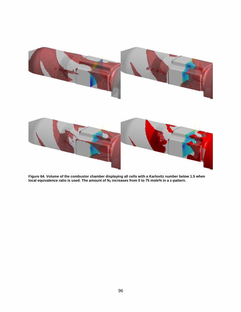
96
Figure 64. Volume of the combustor chamber displaying all cells with a Karlovitz number below 1.5 when local equivalence ratio is used. The amount of N2 increases from 0 to 75 mole% in a z-pattern.

97
Figure 65. Time averaged equivalence ratio profiles on plane normal to the axial direction and with current view facing the burner. Mole% of N2 in the methane based fuel increases in a pattern looking like a 7.
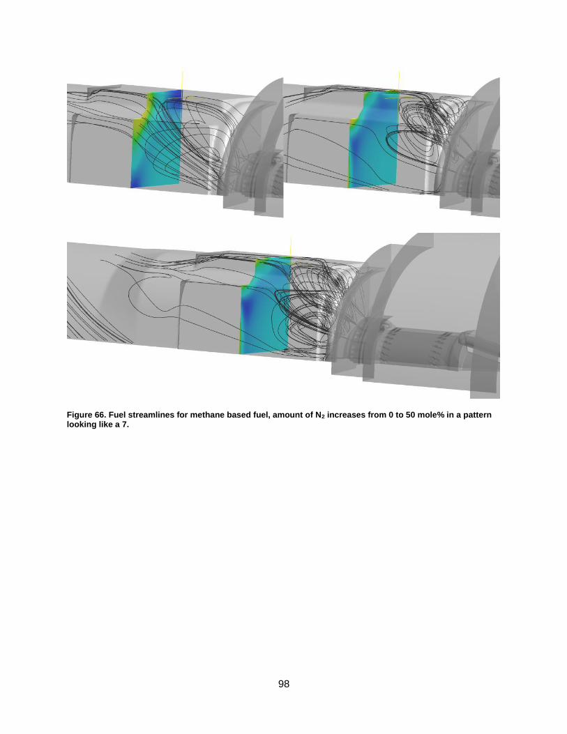
98
Figure 66. Fuel streamlines for methane based fuel, amount of N2 increases from 0 to 50 mole% in a pattern looking like a 7.

99
Figure 67. Time averaged equivalence ratio profiles on plane normal to the axial direction and with current view facing the burner. Mole% of CO2 in the propane based fuel increases in a Z-pattern.
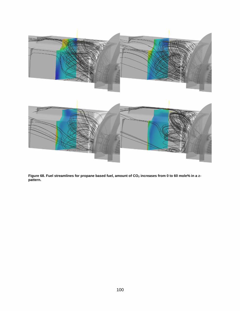
100
Figure 68. Fuel streamlines for propane based fuel, amount of CO2 increases from 0 to 60 mole% in a z-pattern.

101
Figure 69. Time averaged equivalence ratio profiles on plane normal to the axial direction and with current view facing the burner. Mole% of N2 in the propane based fuel increases in a Z-pattern.

102
Figure 70. Fuel streamlines for propane based fuel, amount of N2 increases from 0 to 75 mole% in a z-pattern.