Embed Size (px)
Citation preview

Prediction of Early-Age Cracking of UHPC Materials andStructures: A Thermo-Chemo-Mechanics Approach
by
JongMin Shim
M.S., Korea Advanced Institute of Science of Technology (2001)B.S., Korea Advanced Institute of Science of Technology (1998)
Submitted to the Department of Civil and Environmental Engineeringin partial fulfillment of the requirements for the degree of
Master of Science in Civil and Environmental Engineering
at the
MASSACHUSETTS INSTITUTE OF TECHNOLOGY
February 2005
c° 2005 Massachusetts Institute of Technology. All right reserved.
The author hereby grants to Massachusetts Institute of Technology permission toreproduce and
to distribute copies of this thesis document in whole or in part.
Signature of Author . . . . . . . . . . . . . . . . . . . . . . . . . . . . . . . . . . . . . . . . . . . . . . . . . . . . . . . . . . . . . . . . . . .Department of Civil and Environmental Engineering
February 1, 2005
Certified by . . . . . . . . . . . . . . . . . . . . . . . . . . . . . . . . . . . . . . . . . . . . . . . . . . . . . . . . . . . . . . . . . . . . . . . . . . .Franz-Josef Ulm
Associate Professor of Civil and Environmental EngineeringThesis Supervisor
Accepted by. . . . . . . . . . . . . . . . . . . . . . . . . . . . . . . . . . . . . . . . . . . . . . . . . . . . . . . . . . . . . . . . . . . . . . . . . . .Andrew Whittle
Chairperson, Department Committee on Graduate Studies

Prediction of Early-Age Cracking of UHPC Materials and Structures: A
Thermo-Chemo-Mechanics Approach
by
JongMin Shim
Submitted to the Department of Civil and Environmental Engineeringon February 1, 2005, in partial fulfillment of the
requirements for the degree ofMaster of Science in Civil and Environmental Engineering
Abstract
Ultra-High Performance Concrete [UHPC] has remarkable performance in mechanical proper-ties, ductility, economical benefit, etc., but early-age cracking of UHPC can become an issueduring the manufacturing process due to the high cement content and the highly exothermichydration reaction. Because of the risk of early-age UHPC cracking, there is a need to developa material model that captures the behavior of UHPC at early-ages.
The objective of this research is to develop a new material model for early-age UHPCthrough a thermodynamics approach. The new model is a two-phase thermo-chemo-mechanicalmodel, which is based on two pillars: the first is a hardened two-phase UHPC material model,and the second is a hydration kinetics model for ordinary concrete. The coupling of these twomodels is achieved by considering the evolution of the strength and stiffness properties in thetwo-phase UHPC material model in function of the hydration degree.
The efficiency of the model and finite element implementation is validated with experimentaldata obtained during the casting of a DuctalTM optimized bridge girder. Based on somedecoupling hypothesis, the application of the early-age UHPC model can be carried out in a two-step manner: the thermo-chemical problem is solved first, before solving the two-phase thermo-chemo-mechanical problem. It is shown that the newly developed model is able to accuratelypredict temperature history and deformation behavior of the bridge girder. Furthermore, withthis versatile engineering model, it is possible to predict the risk of cracking, and eventually toreduce it.
Thesis Supervisor: Franz-Josef UlmTitle: Associate Professor of Civil and Environmental Engineering
2

Contents
1 INTRODUCTION 12
1.1 Project Description . . . . . . . . . . . . . . . . . . . . . . . . . . . . . . . . . . . 12
1.2 Research Objective and Approach . . . . . . . . . . . . . . . . . . . . . . . . . . 14
1.3 Outline of Report . . . . . . . . . . . . . . . . . . . . . . . . . . . . . . . . . . . . 16
I BACKGROUND WORKS 18
2 HARDENED UHPC MATERIAL MODEL 19
2.1 Hardened UHPC Material Behavior . . . . . . . . . . . . . . . . . . . . . . . . . 19
2.2 Hardened 1-D UHPC Model . . . . . . . . . . . . . . . . . . . . . . . . . . . . . . 20
2.3 Hardened 3-D UHPC Model . . . . . . . . . . . . . . . . . . . . . . . . . . . . . . 23
2.3.1 The 3-D Constitutive Relations . . . . . . . . . . . . . . . . . . . . . . . . 24
2.3.2 Plasticity of the 3-D Model . . . . . . . . . . . . . . . . . . . . . . . . . . 27
2.3.3 Consistency with the 1-D Model . . . . . . . . . . . . . . . . . . . . . . . 32
2.4 Determination of Hardened Model Parameters . . . . . . . . . . . . . . . . . . . 41
2.4.1 Macroscopic Material Properties . . . . . . . . . . . . . . . . . . . . . . . 41
2.4.2 Review of the Assumptions for the 3-D Model Parameters . . . . . . . . 43
2.4.3 Determination of the 3-D Model Parameters . . . . . . . . . . . . . . . . 44
2.5 Chapter Summary . . . . . . . . . . . . . . . . . . . . . . . . . . . . . . . . . . . 44
3 HYDRATION KINETICS MODEL FOR ORDINARY CONCRETE 46
3.1 Hydration of Cement . . . . . . . . . . . . . . . . . . . . . . . . . . . . . . . . . . 46
3.1.1 Silicate Hydration . . . . . . . . . . . . . . . . . . . . . . . . . . . . . . . 47
3

3.1.2 Aluminate Hydration . . . . . . . . . . . . . . . . . . . . . . . . . . . . . 48
3.2 Macroscopic Modeling of Hydration Reaction for Ordinary Concrete . . . . . . . 48
3.2.1 Simplification of Hydration Reaction Modeling . . . . . . . . . . . . . . . 49
3.2.2 Thermodynamic Framework for Ordinary Concrete at Early Ages . . . . . 50
3.3 Macroscopic Investigation of Hydration Kinetics for Ordinary Concrete . . . . . . 57
3.3.1 Adiabatic Calorimetric Experiment . . . . . . . . . . . . . . . . . . . . . . 57
3.3.2 Isothermal Strength Evolution . . . . . . . . . . . . . . . . . . . . . . . . 58
3.4 Chapter Summary . . . . . . . . . . . . . . . . . . . . . . . . . . . . . . . . . . . 59
II MATERIAL MODELING 60
4 EARLY-AGE UHPC MATERIAL MODEL 61
4.1 Evolving UHPC Material Model . . . . . . . . . . . . . . . . . . . . . . . . . . . 61
4.1.1 Evolution of Strength . . . . . . . . . . . . . . . . . . . . . . . . . . . . . 63
4.1.2 Evolution of Stiffness . . . . . . . . . . . . . . . . . . . . . . . . . . . . . . 64
4.2 Thermodynamic Framework for UHPC at Early Ages . . . . . . . . . . . . . . . 65
4.2.1 Free Energy and State Equations . . . . . . . . . . . . . . . . . . . . . . . 66
4.2.2 Maxwell Symmetries and Decoupling Hypothesis . . . . . . . . . . . . . . 68
4.2.3 Hydration Kinetics and Heat . . . . . . . . . . . . . . . . . . . . . . . . . 71
4.2.4 The 3-D Early-Age Constitutive Relations . . . . . . . . . . . . . . . . . . 72
4.2.5 Plasticity of the 3-D Early-Age Model . . . . . . . . . . . . . . . . . . . . 75
4.2.6 Consistency with the 1-D Model . . . . . . . . . . . . . . . . . . . . . . . 77
4.3 Chapter Summary . . . . . . . . . . . . . . . . . . . . . . . . . . . . . . . . . . . 80
5 FINITE ELEMENT IMPLEMENTATION 81
5.1 Finite Element Formulation . . . . . . . . . . . . . . . . . . . . . . . . . . . . . . 81
5.1.1 Principle of Virtual Displacements . . . . . . . . . . . . . . . . . . . . . . 82
5.1.2 Finite Element Equations . . . . . . . . . . . . . . . . . . . . . . . . . . . 83
5.1.3 Return Mapping Algorithm . . . . . . . . . . . . . . . . . . . . . . . . . . 87
5.2 The EAHC Finite Element Module . . . . . . . . . . . . . . . . . . . . . . . . . . 95
5.2.1 Overview of CESAR-LCPC . . . . . . . . . . . . . . . . . . . . . . . . . 95
4

5.2.2 The EAHC Module . . . . . . . . . . . . . . . . . . . . . . . . . . . . . . 96
5.2.3 Verification of the EAHC Module . . . . . . . . . . . . . . . . . . . . . . . 97
5.3 Chapter Summary . . . . . . . . . . . . . . . . . . . . . . . . . . . . . . . . . . . 105
III ENGINEERING APPLICATION 106
6 EARLY-AGE 3-D UHPC MODEL VALIDATION 107
6.1 Overview of Application . . . . . . . . . . . . . . . . . . . . . . . . . . . . . . . . 107
6.2 Thermo-Chemical Analysis . . . . . . . . . . . . . . . . . . . . . . . . . . . . . . 109
6.2.1 Thermal Boundary Conditions . . . . . . . . . . . . . . . . . . . . . . . . 111
6.2.2 Thermal Properties and Adiabatic Temperature Curve . . . . . . . . . . . 114
6.2.3 Simulation Results and Validation . . . . . . . . . . . . . . . . . . . . . . 117
6.3 Two-Phase Thermo-Chemo-Mechanical Analysis . . . . . . . . . . . . . . . . . . 123
6.3.1 Plane-Section Simulation . . . . . . . . . . . . . . . . . . . . . . . . . . . 123
6.3.2 Mechanical Boundary Conditions . . . . . . . . . . . . . . . . . . . . . . . 125
6.3.3 Mechanical Material Properties . . . . . . . . . . . . . . . . . . . . . . . . 127
6.3.4 Validation . . . . . . . . . . . . . . . . . . . . . . . . . . . . . . . . . . . . 128
6.4 What Caused the Early-Age UHPC Cracking? . . . . . . . . . . . . . . . . . . . 128
6.4.1 Stress and Plastic Strain Distributions . . . . . . . . . . . . . . . . . . . . 131
6.4.2 Stress and Plastic Strain Before and After Applying Prestress . . . . . . . 134
6.4.3 Time History of Simulation Results . . . . . . . . . . . . . . . . . . . . . . 136
6.5 Discussion of Simulation Results . . . . . . . . . . . . . . . . . . . . . . . . . . . 139
6.6 Chapter Summary . . . . . . . . . . . . . . . . . . . . . . . . . . . . . . . . . . . 143
IV CONCLUSIONS 145
7 CONCLUSIONS 146
7.1 Summary of Report . . . . . . . . . . . . . . . . . . . . . . . . . . . . . . . . . . 146
7.2 Future Research . . . . . . . . . . . . . . . . . . . . . . . . . . . . . . . . . . . . 148
A Plastic Projection Schemes For Triaxial Loading 153
5

B Input Format for EAHC Module 155
6
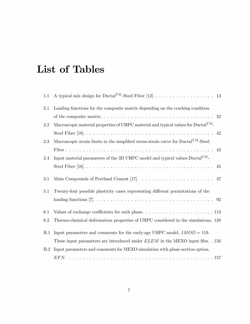
List of Tables
1.1 A typical mix design for DuctalTM -Steel Fiber [12]. . . . . . . . . . . . . . . . . . 13
2.1 Loading functions for the composite matrix depending on the cracking condition
of the composite matrix. . . . . . . . . . . . . . . . . . . . . . . . . . . . . . . . . 32
2.2 Macroscopic material properties of UHPCmaterial and typical values for DuctalTM -
Steel Fiber [18]. . . . . . . . . . . . . . . . . . . . . . . . . . . . . . . . . . . . . . 42
2.3 Macroscopic strain limits in the simplified stress-strain curve for DuctalTM -Steel
Fiber . . . . . . . . . . . . . . . . . . . . . . . . . . . . . . . . . . . . . . . . . . . 42
2.4 Input material parameters of the 3D UHPC model and typical values DuctalTM -
Steel Fiber [18]. . . . . . . . . . . . . . . . . . . . . . . . . . . . . . . . . . . . . . 45
3.1 Main Compounds of Portland Cement [17]. . . . . . . . . . . . . . . . . . . . . . 47
5.1 Twenty-four possible plasticity cases representing different permutations of the
loading functions [7]. . . . . . . . . . . . . . . . . . . . . . . . . . . . . . . . . . . 92
6.1 Values of exchange coefficients for each phase. . . . . . . . . . . . . . . . . . . . . 113
6.2 Thermo-chemical deformation properties of UHPC considered in the simulations. 128
B.1 Input parameters and comments for the early-age UHPC model, IMOD = 119.
These input parameters are introduced under ELEM in the MEXO input files. . 156
B.2 Input parameters and comments for MEXO simulation with plane-section option,
EFN . . . . . . . . . . . . . . . . . . . . . . . . . . . . . . . . . . . . . . . . . . . 157
7

List of Figures
1-1 (a) Comparison of the flexural strength of UHPC (DuctalTM) and Conventional
Concrete (HPC), (b) Enhanced rheology of DuctalTM [12]. . . . . . . . . . . . . . 13
1-2 Construction of the DuctalTM bridge girders at Lexington, Kentucky [9]. . . . . 15
1-3 Early-age cracking observed during casting of on UHPC bridge girder [9]. . . . . 16
2-1 (a) Experimental notched tensile test data of a UHPC material with steel fibers
[5], (b) Stress-displacement response extracted from the test data. . . . . . . . . 20
2-2 Simplified stress-strain curve for the two-phase model. . . . . . . . . . . . . . . . 21
2-3 1D Think Model of a two-phase matrix-fiber composite material for hardened
UHPC. . . . . . . . . . . . . . . . . . . . . . . . . . . . . . . . . . . . . . . . . . . 22
2-4 UHPC strength domain in the Σxx ×Σyy plane (Σzz = 0) [7]. . . . . . . . . . . . 27
2-5 (a) Composite matrix strength domain in the σM,xx × σM,yy plane (σM,zz = 0),
(b) Loading function of the composite matrix before and after cracking [7]. . . . 28
2-6 (a) Composite fiber strength domain in the σF,xx × σF,yy plane (σF,zz = 0), (b)
Loading function of the composite fiber before and after cracking [7]. . . . . . . . 30
2-7 Evolution of composite matrix and composite fiber stresses given by the uniaxial
output from the 3-D hardened UHPC model (in this graph, the subscripts "xx"
are omitted for simplicity) [7]. . . . . . . . . . . . . . . . . . . . . . . . . . . . . . 34
2-8 Comparison of the 1-D and 3-D model output for uniaxial tensile loading [7]. . . 40
2-9 Average notch stress-displacement curve for DuctalTM -Steel Fiber [7]. . . . . . . 42
2-10 Simplified stress-strain curve of UHPC in uniaxial tension and compression. . . . 43
3-1 Diffusion of water through layers of hydrates [25]. . . . . . . . . . . . . . . . . . . 50
8

3-2 Thermo-chemo-mechanical coupling in early-age ordinary concrete and introduc-
tion of decoupling hypothesis. . . . . . . . . . . . . . . . . . . . . . . . . . . . . . 52
4-1 (a) 1-D Think Model of a two-phase matrix-fiber composite material for UHPC
at early-ages, (b) Stress-strain response for UHPC at early ages. . . . . . . . . . 62
4-2 Evolution of strength and stiffness adopted in the modeling of UHPC at early-ages. 64
4-3 Thermo-chemo-mechanical coupling in early-age UHPC and introduction of de-
coupling hypothesis. . . . . . . . . . . . . . . . . . . . . . . . . . . . . . . . . . . 70
4-4 Uniaxial stress-strain behavior obtained from the analytical solution: (a) Entire
stress-strain curve, (b) Focus on first cracking behavior. . . . . . . . . . . . . . . 79
5-1 Overview of the CESAR-LCPC program structure. . . . . . . . . . . . . . . . . . 95
5-2 Overview of the subroutine structure of the main solver, program CESAR. . . . . 96
5-3 Flow chart of the subroutine EXMEXO and corresponding variables to be dealt
with. . . . . . . . . . . . . . . . . . . . . . . . . . . . . . . . . . . . . . . . . . . . 98
5-4 Flow chart of the subroutine EXMEXO and corresponding subroutines, where
italic letters indicate newly developed subroutines for the EAHC module. . . . . 99
5-5 Mesh design and boundary conditions of the uniaxial tension test simulation
using axisymmetric elements: (a) Single element, (b) Fifty elements. . . . . . . . 100
5-6 ξ = 0.25: uniaxial response of finite element simulations compared with the
analytical simulations: (a) Entire stress-strain curve, (b) Focus on first cracking
behavior. . . . . . . . . . . . . . . . . . . . . . . . . . . . . . . . . . . . . . . . . 101
5-7 ξ = 0.5: uniaxial response of finite element simulations compared with the an-
alytical simulations: (a) Entire stress-strain curve, (b) Focus on first cracking
behavior. . . . . . . . . . . . . . . . . . . . . . . . . . . . . . . . . . . . . . . . . 102
5-8 ξ = 0.5: uniaxial response of finite element simulations compared with the an-
alytical simulations: (a) Entire stress-strain curve, (b) Focus on first cracking
behavior. . . . . . . . . . . . . . . . . . . . . . . . . . . . . . . . . . . . . . . . . 103
5-9 ξ = 1.0: uniaxial response of finite element simulations compared with the an-
alytical simulations: (a) Entire stress-strain curve, (b) Focus on first cracking
behavior. . . . . . . . . . . . . . . . . . . . . . . . . . . . . . . . . . . . . . . . . 104
9
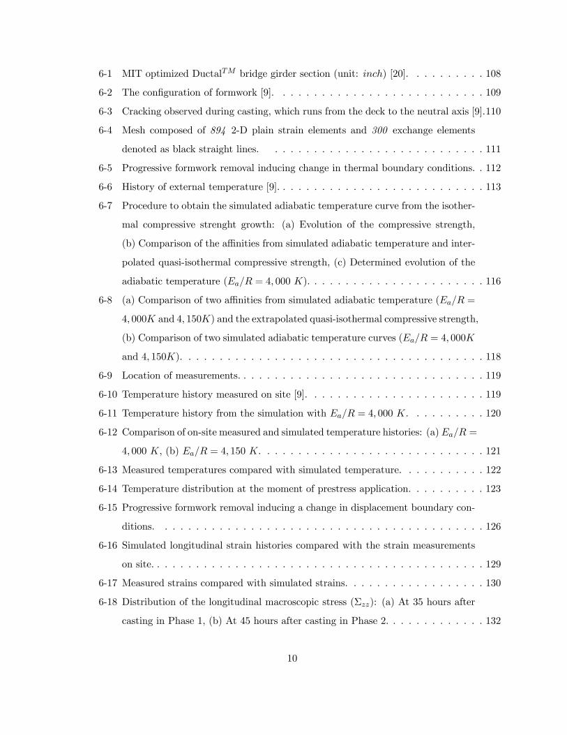
6-1 MIT optimized DuctalTM bridge girder section (unit: inch) [20]. . . . . . . . . . 108
6-2 The configuration of formwork [9]. . . . . . . . . . . . . . . . . . . . . . . . . . . 109
6-3 Cracking observed during casting, which runs from the deck to the neutral axis [9].110
6-4 Mesh composed of 894 2-D plain strain elements and 300 exchange elements
denoted as black straight lines. . . . . . . . . . . . . . . . . . . . . . . . . . . . 111
6-5 Progressive formwork removal inducing change in thermal boundary conditions. . 112
6-6 History of external temperature [9]. . . . . . . . . . . . . . . . . . . . . . . . . . . 113
6-7 Procedure to obtain the simulated adiabatic temperature curve from the isother-
mal compressive strenght growth: (a) Evolution of the compressive strength,
(b) Comparison of the affinities from simulated adiabatic temperature and inter-
polated quasi-isothermal compressive strength, (c) Determined evolution of the
adiabatic temperature (Ea/R = 4, 000 K). . . . . . . . . . . . . . . . . . . . . . . 116
6-8 (a) Comparison of two affinities from simulated adiabatic temperature (Ea/R =
4, 000K and 4, 150K) and the extrapolated quasi-isothermal compressive strength,
(b) Comparison of two simulated adiabatic temperature curves (Ea/R = 4, 000K
and 4, 150K). . . . . . . . . . . . . . . . . . . . . . . . . . . . . . . . . . . . . . . 118
6-9 Location of measurements. . . . . . . . . . . . . . . . . . . . . . . . . . . . . . . . 119
6-10 Temperature history measured on site [9]. . . . . . . . . . . . . . . . . . . . . . . 119
6-11 Temperature history from the simulation with Ea/R = 4, 000 K. . . . . . . . . . 120
6-12 Comparison of on-site measured and simulated temperature histories: (a)Ea/R =
4, 000 K, (b) Ea/R = 4, 150 K. . . . . . . . . . . . . . . . . . . . . . . . . . . . . 121
6-13 Measured temperatures compared with simulated temperature. . . . . . . . . . . 122
6-14 Temperature distribution at the moment of prestress application. . . . . . . . . . 123
6-15 Progressive formwork removal inducing a change in displacement boundary con-
ditions. . . . . . . . . . . . . . . . . . . . . . . . . . . . . . . . . . . . . . . . . . 126
6-16 Simulated longitudinal strain histories compared with the strain measurements
on site. . . . . . . . . . . . . . . . . . . . . . . . . . . . . . . . . . . . . . . . . . . 129
6-17 Measured strains compared with simulated strains. . . . . . . . . . . . . . . . . . 130
6-18 Distribution of the longitudinal macroscopic stress (Σzz): (a) At 35 hours after
casting in Phase 1, (b) At 45 hours after casting in Phase 2. . . . . . . . . . . . . 132
10

6-19 Distribution of the longitudinal macroscopic stress (Σzz): (a) Before prestress
application (Phase 3), (b) After prestress application (Phase 4). . . . . . . . . . . 133
6-20 Distribution of the longitudinal plastic strain in the composite matrix (εpM,zz) at
both 35 and 45 hours after casting in Phase 1 and 2, respectively. . . . . . . . . 134
6-21 Distribution of the longitudinal plastic strain in the composite matrix (εpM,zz) in
the web (left) and the deck (right) before and after presstress application. . . . . 135
6-22 (a) Longitudinal macroscopic stress profile along the web, (b) Longitudinal plas-
tic strain in the composite matrix along the web. . . . . . . . . . . . . . . . . . . 137
6-23 (a) Longitudinal macroscopic stress profile in the deck, (b) Longitudinal plastic
strain in the composite matrix in the deck. . . . . . . . . . . . . . . . . . . . . . 138
6-24 (a) Time history of the longitudinal macroscopic stresses, (b) Time history of
the longitudinal plastic strains in the composite matrix [The marked triangular
points indicate the following: A= inner-form removal, B=outer-form removal
and C=prestress application]. . . . . . . . . . . . . . . . . . . . . . . . . . . . . . 140
6-25 (a) A lateral shot of the girder 21 m long, (b) A full scale girder is removed from
the formwork [9]. . . . . . . . . . . . . . . . . . . . . . . . . . . . . . . . . . . . . 141
6-26 Comparison of the longitudinal plastic strains in the composite matrix along the
deck. . . . . . . . . . . . . . . . . . . . . . . . . . . . . . . . . . . . . . . . . . . . 142
11

Chapter 1
INTRODUCTION
1.1 Project Description
Ultra-High Performance Concrete [UHPC] is a new generation of fiber reinforced cementi-
tious materials with enhanced mechanical and aesthetic properties. An example of UHPC is
DuctalTM , made by Lafarge, shown in Figure 1-1. It is composed of 710 kg/m3 of cement and
160 kg/m3 of steel fibers. Moreover, it has a very low water cement ratio of roughly 20 %,
and superplasticizer is employed in this material to ensure workability. A typical mix design
for DuctalTM -Steel Fiber is given in Table 1.1. Its remarkable properties can be summarized
as follows:
• It has 3− 7 times the compressive, flexural, and tensile strength of normal concrete;
• It behaves as an elasto-plastic ductile material in tension;
• It allows smaller section sizes which do not require secondary steel reinforcement;
• It has high workability which enables structural elements to be cast in any shape.
Thus, UHPC eventually enables the reduction of global construction costs by using less
materials, allowing faster construction, reducing labour, reducing maintenance, increasing usage
life, etc. However, due to the high cement content and highly exothermal hydration reaction,
early-age cracking can become an issue during the manufacturing process.
12

(a) (b)
Figure 1-1: (a) Comparison of the flexural strength of UHPC (DuctalTM) and ConventionalConcrete (HPC), (b) Enhanced rheology of DuctalTM [12].
MaterialMass/Volume
[kg/m3]Mass Ratio
Cement 710 1.000Silica Fume 230 0.324
Ground Quartz 210 0.296Sand 1020 1.437
Metallic Fibers 160 0.225Superplasticizer 13 0.018
Water 140 0.197
Table 1.1: A typical mix design for DuctalTM -Steel Fiber [12].
13

As a part of a UHPC bridge development program, Prestress Service Inc. [PSi] cast four
DuctalTM optimized bridge girders at Lexington, Kentucky. These tests were carried out under
contract of the Federal Highway Administration [FHWA] over the period of October 11, 2003
to January 31, 2004 (Figure 1-2). The optimized girder section was developed at MIT using a
model-based simulation approach [18], with the collaboration of FHWA, PSi and Lafarge North
America. During casting of the girders, early-age cracks were observed, and one of them is
shown in Figure 1-3. Thus, it becomes clear that an accurate modeling of the behavior of
UHPC at early ages is necessary to avoid early-age cracking, which affects the durability of
UHPC structures.
1.2 Research Objective and Approach
The ultimate industrial goal of this research is the prevention of early-age cracking in UHPC
structures. The first step toward this goal is to predict when and where early-age cracking
occurs in a structure so that one can reduce the risk of cracking. To reach this goal, there is
a necessity to develop a material model which captures the behavior of UHPC at early ages.
This development, which is focus of this research, is based on two previous developments: a
hardened UHPC material model and a hydration kinetics model.
More precisely, a two-phase constitutive model for hardened UHPC materials has been
recently developed at MIT [7]. This nonlinear constitutive model for UHPC was implemented in
a commercial finite element program, CESAR-LCPC, and validated for 2-D and 3-D structures
[7] [21]. The model has been also used for the design of a prototype UHPC highway bridge
girder for the U.S. market place [18].
Hydration of concrete is a highly exothermic and thermally activated reaction, so that a
thermochemical model is necessary for the modeling of hydration reaction. A simple hydration
kinetics model for ordinary early-age concrete is the one developed by Ulm and Coussy [25]
[26]. In this model, it is assumed that the diffusion of water through the layers of hydrates
is the dominant mechanism of the hydration kinetics. The hydration process of concrete is
viewed, from a macroscopic perspective, as a single chemical reaction in which the free water
is a reactant phase that combines with the unhydrated phase to form solid material.
14

Figure 1-2: Construction of the DuctalTM bridge girders at Lexington, Kentucky [9].
15

Figure 1-3: Early-age cracking observed during casting of on UHPC bridge girder [9].
Given these backgrounds, the objective of the presented research is to develop a new material
model for early-age UHPC, which combines these two approaches: the MIT-UHPC model and
the Ulm-Coussy hydration model. In order to achieve the research objectives, the following
tasks need to be performed:
1. To understand the hardened UHPC material model;
2. To combine the hydration kinetics model with the hardened UHPC material model;
3. To implement the new material model into a finite element program;
4. To validate the proposed material model through an application to a UHPC structure.
1.3 Outline of Report
This report is divided into seven chapters, starting with the hardened UHPC material model
and the hydration kinetics model, moving on to the development of the novel early-age UHPC
material model and its finite element implementation, and finishing with the validation of the
proposed model.
16

Chapter 2 begins with a brief review of the two-phase hardened UHPC material model.
The two-phase model reflects the material composition with one phase representing the matrix
and the other representing the reinforcing fibers. This separation of the overall composite
behavior into individual matrix and fiber phases is very effective because the plastic strain in
the composite matrix is used to represent the cracking in the UHPC material.
Chapter 3 reviews the hydration kinetics model for ordinary concrete. One important
assumption of this kinetics model is the decoupling hypothesis, which neglects the effect of
mechanical change on the thermal and chemical process.
In Chapter 4, the newly developed early-age UHPC material model is presented in detail.
The coupling of the two mentioned models requires to consider the evolution of the strength
and stiffness properties in the two-phase UHPC material model.
Chapter 5 presents details of the implementation of the early-age UHPC models in a fi-
nite element environment. The implementation is verified for consistency and stability with
respect to analytical models and mesh size to demonstrate the viability of the finite element
implementation.
Chapter 6 is devoted to structural simulations using the finite element program. The effec-
tiveness of the model and finite element program is validated with experimental data. Thanks
to the decoupling hypothesis, the application of the early-age UHPC model is carried out in
a two-step manner: thermo-chemical problem and then two-phase thermo-chemo-mechanical
problem. In this Chapter, the simulation results from both problems are compared with
experimental data from the Kentucky casting.
Finally, Chapter 7 summarizes the results of this project, and discusses current limitations
and suggestions for future research.
17

Part I
BACKGROUND WORKS
18

Chapter 2
HARDENED UHPC MATERIAL
MODEL
One of the great benefits of UHPC is that it shows considerable tensile strength that can be
taken into account in the design of UHPC structures. Thus, the tensile behavior of UHPC
needs to be captured correctly in a UHPC constitutive model. This Chapter reviews the UHPC
material model that has been developed at MIT [7]. The model is a two-phase model; one phase
representing the matrix and the other phase representing the reinforcing fibers. In addition,
the matrix-fiber interaction is taken into account as an internal coupling effect between the
irreversible deformation of the composite constituents.
2.1 Hardened UHPC Material Behavior
A typical tensile response of hardened UHPC is shown in Figure 2-1 (a). It can be simplified into
four domains shown in Figure 2-1 (b); first a linear elastic behavior, second a brittle strength
drop, third a post-cracking behavior, and fourth a composite yielding. Figure 2-2 shows the
simplified macroscopic stress-strain behavior of UHPC (macroscopic stress, Σ, and macroscopic
strain, E) and the evolution of the matrix and the fiber stresses ( σF and σM ) for the modeling
of UHPC. This simplified stress-strain behavior can be described by the following three stages:
1. Initial Elasticity: When the composite is first loaded, UHPC behaves elastically with a
stiffness of K0 until the composite stress reaches an initial tensile strength Σ−t,1. At this
19

0.0
2.0
4.0
6.0
8.0
10.0
0 0.05 0.1 0.15 0.2 0.25 0.3Displacement [mm]
Ave
rage
Not
ch S
tres
s [M
Pa]
0.0
2.0
4.0
6.0
8.0
10.0
0 0.05 0.1 0.15 0.2 0.25 0.3Displacement [mm]
Ave
rage
Not
ch S
tres
s [M
Pa]
0.0
2.0
4.0
6.0
8.0
10.0
0 0.05 0.1 0.15 0.2 0.25 0.3Displacement [mm]
Ave
rage
Not
ch S
tres
s [M
Pa]
0.0
2.0
4.0
6.0
8.0
10.0
0 0.05 0.1 0.15 0.2 0.25 0.3Displacement [mm]
Ave
rage
Not
ch S
tres
s [M
Pa]
0.0
2.0
4.0
6.0
8.0
10.0
0 0.05 0.1 0.15 0.2 0.25 0.3Displacement [mm]
Ave
rage
Not
ch S
tres
s [M
Pa]
(a) (b)
Figure 2-1: (a) Experimental notched tensile test data of a UHPC material with steel fibers [5],(b) Stress-displacement response extracted from the test data.
point, significant cracking in the matrix develops causing a stress drop to a post-cracking
tensile strength Σ+t,1.
2. Post-cracking Behavior: After the matrix cracks, there is a second linear behavior with a
stiffness of K1 until the fibers start to yield.
3. Yielding and Failure: Finally, the composite yields and ultimately fails at an ultimate
tensile yield strength Σt,2. Tension softening behavior is neglected in the material model.
The complex tensile behavior is condensed into five macroscopic material properties (K0,
K1, Σ−t,1, Σ+t,1, and Σt,2), which can be extracted from tensile test data.
2.2 Hardened 1-D UHPC Model
In order to represent the simplified UHPC material behavior, Chuang and Ulm [8] proposed the
1-D Think Model displayed in Figure 2-3. In this model, matrix and fiber phases are modeled
as separate phases with the same macroscopic strain, E, but with different stress states, σM
and σF . In turn, the macroscopic stress, Σ, is always the sum of the composite matrix stress,
σM , and the composite fiber stress, σF .
20

K0(CM,CF) K1(CM,CF,M)
Matrix Stress
1E 2E
,1t+Σ
,1t−Σ
t Mf k+F yfσ =
M Mkσ =
,2tΣ
E
Σ
Fiber Stress
K0(CM,CF) K1(CM,CF,M)
Matrix Stress
1E 2E
,1t+Σ
,1t−Σ
t Mf k+F yfσ =
M Mkσ =
,2tΣ
E
Σ
Fiber Stress
Figure 2-2: Simplified stress-strain curve for the two-phase model.
The macroscopic material model is composed of three parts: a brittle-plastic matrix phase,
an elasto-plastic fiber phase and an elastic coupling spring. The matrix phase consists of an
elastic spring of stiffness CM , a tensile plate element of strength ft, and a frictional element
of strength kM . From a micro-mechanical point of view, the elastic spring represents the
elastic contribution of the matrix, the plate device represents the brittle behavior of the matrix
and the frictional device represents the fracture resistance of the matrix. The fiber phase
behavior is represented by an elastic spring of stiffness CF , and a frictional element of strength
fy. The elastic spring represents the elastic contribution of the fibers and the friction element
can be associated with the plastic pullout behavior of the fibers during composite yielding. In
addition, the two parallel phases are coupled by an elastic spring of stiffnessM , which links the
irreversible matrix behavior (plastic strain εpM) with the irreversible reinforcing fiber behavior
(plastic strain εpF ). At the micro-scale, this elastic coupling can be associated with a possible
shear stress transfer from the matrix to the fiber over their interface, and intact matrix ligaments
which transfer stresses even after cracking. The 6 model parameters (CM , CF , M , ft, kM and
fy) govern the tensile behavior of the composite material.
While a single tensile stress-strain relation provides five macroscopic material properties
21

Fσ σΜΣ= +
pMε
pFεyf
tf
MC
E
FCMk
M
Fσ σΜΣ= +
pMε
pFεyf
tf
MC
E
FCMk
M
Figure 2-3: 1D Think Model of a two-phase matrix-fiber composite material for hardenedUHPC.
(K0, K1, Σ−t,1, Σ+t,1 and Σt,2), the composite model involves six model parameters (CM , CF ,M ,
ft, kM and fy). They are related by the following equations:
K0 = CM + CF
K1 = CF +CMMCM+M
(2.1)
Σ−t,1 =³1 + CF
CM
´(ft + kM) with E−1 =
ft+kMCM
Σ+t,1 = Σ−t,1 − CM
CM+Mft with E+1 =
ft+kMCM
Σt,2 = fy + kM with E2 =kMM+fy(CM+M)CF (CM+M)+CMM
(2.2)
Thus, in order to close the identification problem of model parameters, another relation is
required. A typical UHPC material has a characteristic low fiber volume fraction, cF =VFV ≤
6%. For cF ≤ 6% and typical elastic moduli of the matrix and the fiber phases, the composite
stiffness ratio, κ = CFCM, shows the following range of values:
0.02 ≤ κ ≤ 0.13 (2.3)
22

Thus, the six model parameters can be practically obtained by an asymptotic analysis, setting
the composite stiffness ratio κ→ 0. Then, (2.1) and (2.2) reduce to:
K0 ' CM
K1 ' CMMCM+M
(2.4)
Σ−t,1 ' ft + kM with E−1 =ft+kMCM
Σ+t,1 ' kM with E+1 =ft+kMCM
Σt,2 = fy + kM with E2 ' kMM+fy(CM+M)CMM
(2.5)
2.3 Hardened 3-D UHPC Model
The 1-D Think Model has the ability to continuously model the stress-strain behavior of UHPC
materials while capturing the micro-mechanical behavior of the composite material. Since
the UHPC material model is a macroscopic model, the extension to 3-D is straightforward,
essentially requiring to substitute for 1-D macroscopic parameters and functions with their 3-D
counterparts. The 3-D macroscopic model is constructed around three main components:
• The 3-D constitutive relations: The 3-D stress-strain relation is derived from the energy
consideration for a stress-strain expression which is thermodynamically consistent with
the 1-D result.
• Plasticity of the 3-D model: The 3-D failure criteria and the corresponding plastic flow
rules are considered. The 3-D loading functions require 3-D strength limits, i.e. tension,
compression, shear, etc. An associated plastic flow rule is adopted.
• Consistency with the 1-D model: The uniaxial behavior of the 3-D model is calibrated
with the 1-D model so that the 3-D model gives tension output which is consistent with
that of the 1-D model.
These different components, developed in detail in [7], are briefly recalled below.
23

2.3.1 The 3-D Constitutive Relations
The starting point of the 3-D model is the Clausius-Duhem inequality, which for isothermal
conditions reads [24]:
ϕdt = Σ : dE− dΨ ≥ 0 (2.6)
where ϕdt stands for the dissipation; Σ and E are the 2nd order macroscopic stress tensor and
macroscopic strain tensor, respectively; and Ψ is the free energy. For UHPC materials, using
the elastic contribution of the different springs in Figure 2-3, the free energy reads:
Ψ = Ψ¡E, εpM , εpF
¢(2.7)
=1
2
¡E− εpM
¢: CM :
¡E− εpM
¢+1
2
¡E− εpF
¢: CF :
¡E− εpF
¢+1
2
¡εpM − ε
pF
¢: M :
¡εpM − ε
pF
¢where CM , CF , andM are the 4th order stiffness tensors of the composite matrix, the composite
fiber, and the matrix-fiber coupling, respectively. Use of (2.7) in (2.6) yields the incremental
form of the general 3-D stress-strain relations, which is an incremental form read:
⎧⎪⎪⎪⎨⎪⎪⎪⎩dΣ
dσM
dσF
⎫⎪⎪⎪⎬⎪⎪⎪⎭ =
⎡⎢⎢⎢⎣CM CF
CM +M −M
−M CF +M
⎤⎥⎥⎥⎦ :⎧⎨⎩ dE− dεpM
dE− dεpF
⎫⎬⎭ (2.8)
We verify that the macroscopic stress, Σ, is always the sum of the matrix stress, σM , and fiber
stress, σF :
dΣ = dσM + dσF (2.9)
= (CM +M) :¡dE− dεpM
¢−M :
¡dE− dεpF
¢+(CF +M) :
¡dE− dεpF
¢−M :
¡dE− dεpM
¢The general 3-D constitutive model with matrix-fiber interaction involves 3 × 21 stiffness
parameters associated with the stiffness tensors, CM , CF , and M. In a first approach to
24

UHPC materials with random fiber orientation, the behavior can be assumed to be isotropic.
Similarly, using the assumption of randomly oriented cracks after matrix cracking, the post-
cracking stiffness behavior of the modeled material can also be approximated as isotropic. In
this case, the stiffness tensors can be described with two unique scalar values:
CM = 3KMK+2GMJ
CF = 3KFK+2GFJ
M = 3KIK+2GIJ
(2.10)
where K =Kijkl =13δijδkl is the volumetric part of the 4
th order unit tensor I, and J = I − K
is the deviatoric part 1. KM , KF and KI are the bulk moduli of the composite matrix, the
composite fiber and the matrix-fiber coupling; GM , GF and GI are the shear moduli of the
composite matrix, the composite fiber and the matrix-fiber coupling. The bulk moduli and the
shear moduli are related to elastic moduli of the composite matrix, CM , the composite fiber,
CF , and matrix-fiber coupling, M , by:
KM = CM3(1−2νM ) ; GM = CM
2(1+νM );
KF =CF
3(1−2νF ) ; GF =CF
2(1+νF );
KI =M3D
3(1−2νI) ; GI =M3D
2(1+νI)
(2.11)
where νM , νF and νI are the Poisson’s ratios of the composite matrix, the composite fiber and
the matrix-fiber coupling, respectively; andM3D is the 3-D counterpart of M in the 1-D model
(Figure 2-3). However, unlike the composite matrix stiffness and the composite fiber stiffness,
the 3-D coupling stiffness tensor M is not directly related to its 1-D counterpart M . The 3-D
coupling stiffness tensor must be formulated in such a way that the 3-D model gives the same
macroscopic uniaxial response as the 1-D model, as detailed later on.
1The symmetric 4th order tensors can be written in the following matrix forms:
I =
⎡⎢⎢⎢⎢⎢⎢⎣1 0 0 0 0 00 1 0 0 0 00 0 1 0 0 00 0 0 1 0 00 0 0 0 1 00 0 0 0 0 1
⎤⎥⎥⎥⎥⎥⎥⎦ ; K =
⎡⎢⎢⎢⎢⎢⎢⎣
13
13
13
0 0 013
13
13
0 0 013
13
13 0 0 0
0 0 0 0 0 00 0 0 0 0 00 0 0 0 0 0
⎤⎥⎥⎥⎥⎥⎥⎦ ; J =
⎡⎢⎢⎢⎢⎢⎢⎣
23
− 13
− 13
0 0 0− 13
23
− 13
0 0 0− 13 − 1
323 0 0 0
0 0 0 1 0 00 0 0 0 1 00 0 0 0 0 1
⎤⎥⎥⎥⎥⎥⎥⎦
25

Equation (2.8) can be restated in an isotropic format:
dΣ =dΣv1+dΣd
dσM = dσvM1+ dsM
dσF = dσvF1+dsF
(2.12)
where 1 is the 2nd order unit tensor; dΣv = 13tr (dΣ), dσ
vM = 1
3 tr (dσM) and dσvF =13tr (dσF )
are volumetric stress increments; and dΣd, dsM and dsF are deviatoric stress increments. The
volumetric stress-strains are represented by:
⎧⎪⎪⎪⎨⎪⎪⎪⎩dΣv
dσvM
dσvF
⎫⎪⎪⎪⎬⎪⎪⎪⎭ = 3
⎡⎢⎢⎢⎣KM KF
KM +KI −KI
−KI KF +KI
⎤⎥⎥⎥⎦⎧⎨⎩ dEv − d p
M
dEv − d pF
⎫⎬⎭ (2.13)
where dEv = 13 tr (dE), d
pM = 1
3tr¡dεpM
¢and d p
F =13tr¡dεpF
¢are volumetric strain increments.
Similarly, the deviatoric stress-strain relations are given by:
⎧⎪⎪⎪⎨⎪⎪⎪⎩dΣd
dsM
dsF
⎫⎪⎪⎪⎬⎪⎪⎪⎭ = 2
⎡⎢⎢⎢⎣GM GF
GM +GI −GI
−GI GF +GI
⎤⎥⎥⎥⎦ :⎧⎨⎩ dEd − depM
dEd − depF
⎫⎬⎭ (2.14)
where dEd = dE − dEv1, depM = dεpM − d pM1 and depF = dεpF − d p
F1 are deviatoric strain
increments.
In a randomly oriented fiber system, there are six composite elastic properties to be deter-
mined. Four of them (GM , GF , νM and νF ) are associated with the elasticity of the matrix
and the fiber, and they are parameters that relate to the elastic composite matrix behavior.
However, two of them (M3D and νI) are associated with the elasticity of the matrix-fiber cou-
pling, and they are the constants related to the irreversible composite matrix behavior, i.e.
post-cracking behavior. Thus, it is first necessary to consider the strength domain and post-
cracking plasticity behavior of the model in order to obtain meaningful expressions forM3Dand
νI .
26

Figure 2-4: UHPC strength domain in the Σxx ×Σyy plane (Σzz = 0) [7].
2.3.2 Plasticity of the 3-D Model
The 3-D Strength Domain
The UHPC strength domain is characterized by two different strength limits, an initial limit
and a yield limit. This triaxial strength domain can be captured by 6 macroscopic strength
values, as shown in Figure 2-4, represented by the following: (1) initial tensile strength, Σ−t,1;
(2) initial compressive strength, Σ−c,1; (3) initial biaxial compressive strength, Σ−b,1; (4) tensile
yield strength, Σt,2; (5) compressive yield strength, Σc,2; (6) biaxial compressive yield strength,
Σb,2.
From a modeling point of view, the strength domain DE of UHPC, which is described by
the 3-D loading function F , is governed by the individual behaviors of the composite matrix
and the composite fiber:
Σ ∈ DE ⇔ F = max [FM , FF ] ≤ 0 ⇔*σM ∈ DM ⇔ FM (σM) ≤ 0
σF ∈ DF ⇔ FF (σF ) ≤ 0
+(2.15)
where DM and DF are the strength domains of the matrix and the fiber; FM and FF are the
27

(a) (b)
Figure 2-5: (a) Composite matrix strength domain in the σM,xx×σM,yy plane (σM,zz = 0), (b)Loading function of the composite matrix before and after cracking [7].
3-D loading function of the matrix and the fiber, respectively.
The composite matrix strength domain The elasto-brittle-plastic behavior of the matrix
phase is captured by the matrix strength domain with a higher initial limit and a lower yield
limit. This strength domain is depicted by 6 characteristic values shown in Figure 2-5 (a):
1. The initial tensile strength, σMt. This is the same as the matrix cracking strength of the
1-D UHPC model, σMt = ft + kM .
2. The initial compressive strength, σMc.
3. The initial biaxial compressive strength, σMb.
4. The tensile post-cracking yield strength, σcrMt. This is equivalent to the matrix post-
cracking strength of the 1-D UHPC model, σcrMt = kM .
5. The compressive yield strength, σcrMc.
6. The biaxial compressive yield strength, σcrMb.
Before matrix cracking, the initial strength parameters govern the loading function of the
composite matrix. To describe these initial strength limits, a tension cut-off [TC] criterion is
28

considered to capture the tension-tension stress states³fTC,0M
´; a Drucker-Prager [DP] criterion
is considered for the compression-tension stress states³fUN,0M
´; and another DP criterion is
considered for the compression-compression stress states³fBI,0M
´. The initial loading functions
read:fTC,0M = I1,M − σMt ≤ 0
fUN,0M = αUNM I1,M + |sM |− cUN,0
M ≤ 0
fBI,0M = αBIM I1,M + |sM |− cBI,0M ≤ 0
(2.16)
where
I1,M = trσM (2.17)
αUNM =
√2/3(σMc−σMc)
σMc+σMc; cUN,0
M =³q
23 − σUNM
´σMc;
αBIM =
√2/3(σMb−σMc)
2σMb−σMc; cBI,0M =
³q23 − σBIM
´σMc
(2.18)
After cracking, the post-cracking strength parameters govern the loading function of the
composite matrix. In order to reduce modeling parameters, it is assumed that the post-cracking
composite strengths are reduced by the same factor:
γcr =σcrMt
σMt=
σcrMc
σMc=
σcrMb
σMb(2.19)
where the superscript "cr" denotes a cracked state. Now, the post-cracking loading functions
read:fTC,crM = I1,M − σcrMt ≤ 0
fUN,crM = αUNM I1,M + |sM |− cUN,cr
M ≤ 0
fBI,crM = αBIM I1,M + |sM |− cBI,crM ≤ 0
(2.20)
where
cUN,crM = γcrcUN,0
M ; cBI,crM = γcrcBI,0M(2.21)
These loading functions are illustrated in Figure 2-5 (b) in the I1 − |s| plane. In summary, we
can describe the strength domain of the composite matrix as follows:
σM ∈ DM ⇔ FM (σM) =
*F 0M = max
hfTC,0M , fUN,0
M , fBI,0M
ibefore cracking
F crM = max
hfTC,crM , fUN,cr
M , fBI,crM
iafter cracking
+≤ 0
(2.22)
29
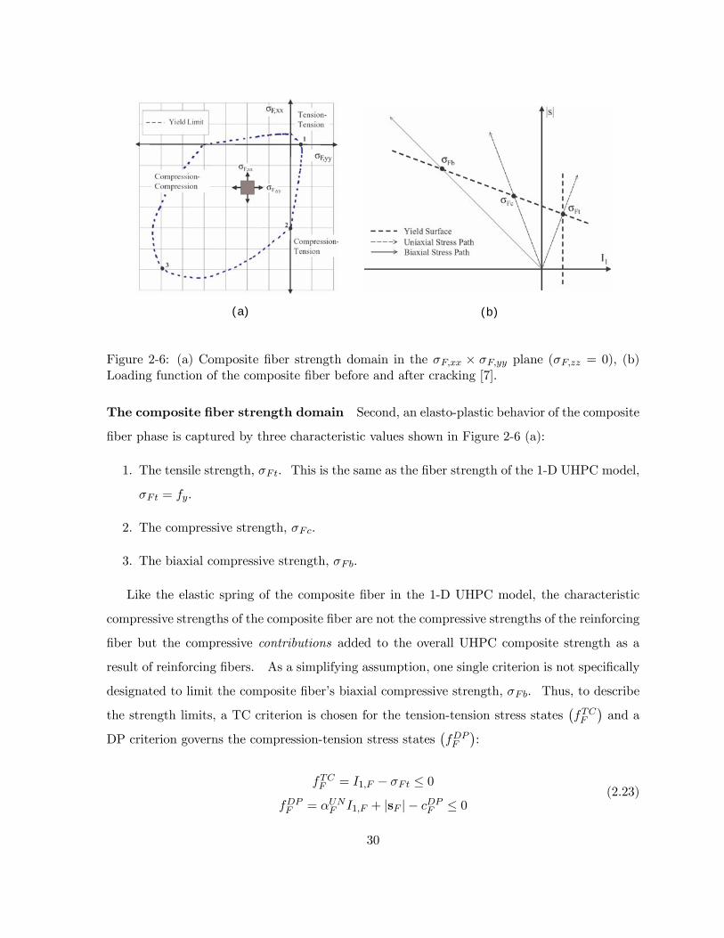
(a) (b)
Figure 2-6: (a) Composite fiber strength domain in the σF,xx × σF,yy plane (σF,zz = 0), (b)Loading function of the composite fiber before and after cracking [7].
The composite fiber strength domain Second, an elasto-plastic behavior of the composite
fiber phase is captured by three characteristic values shown in Figure 2-6 (a):
1. The tensile strength, σFt. This is the same as the fiber strength of the 1-D UHPC model,
σFt = fy.
2. The compressive strength, σFc.
3. The biaxial compressive strength, σFb.
Like the elastic spring of the composite fiber in the 1-D UHPC model, the characteristic
compressive strengths of the composite fiber are not the compressive strengths of the reinforcing
fiber but the compressive contributions added to the overall UHPC composite strength as a
result of reinforcing fibers. As a simplifying assumption, one single criterion is not specifically
designated to limit the composite fiber’s biaxial compressive strength, σFb. Thus, to describe
the strength limits, a TC criterion is chosen for the tension-tension stress states¡fTCF
¢and a
DP criterion governs the compression-tension stress states¡fDPF
¢:
fTCF = I1,F − σFt ≤ 0
fDPF = αUNF I1,F + |sF |− cDP
F ≤ 0(2.23)
30

where
I1,F = trσF (2.24)
αDPF =
√2/3(σFc−σFc)σFc+σFc
; cDPF =
³p2/3− σDP
F
´σFc; (2.25)
With these relations, we can describe the strength domain of the composite fiber as follows:
σF ∈ DF ⇔ FF (σF ) = max£fTCF , fDP
F
¤≤ 0 (2.26)
Plastic Flow Rule
The composite matrix and composite fiber are both governed by the following Kuhn-Tucker
conditions:
FM (σM) ≤ 0; dλM ≥ 0; FM (σM) dλM = 0 (2.27)
FF (σF ) ≤ 0; dλF ≥ 0; FF (σF ) dλF = 0 (2.28)
where dλM and dλF are the plastic multipliers that represent the intensity of the plastic yielding
in the composite matrix and the composite fiber, respectively. In this study, an associated
plastic flow rule is adopted, so that plastic deformations occurs in the normal direction to the
loading function ( ∂FM∂σMand ∂FF
∂σF). Since the two types of loading function (TC and DP) are
used to describe the plasticity of the early-age UHPC, the direction of the plastic flow for each
loading function now reads:
∂fTC (σ)
∂σ= 1;
∂fDP (σ)
∂σ= α1+Ns (2.29)
where Ns =s|s| is the normalized deviatoric stress tensor. Now, the permanent deformations
of the composite matrix and the composite fiber read:
dεpM =Xi
dλM,i∂FM,i (σM , ξ)
∂σM(2.30)
= dλTCM∂fTCM
∂σM+ dλUNM
∂fUNM
∂σM+ dλBIM
∂fBIM
∂σM
= dλTCM 1+ dλUNM£αUNM 1+NsM
¤+ dλBIM
£αBIM 1+NsM
¤
31

Before Matrix Cracking After Matrix Cracking
fTCM = fTC,0M fTC,crM
fUNM = fUN,0M fUN,cr
M
fBIM = fBI,0M fBI,crM
Table 2.1: Loading functions for the composite matrix depending on the cracking condition ofthe composite matrix.
dεpF =Xi
dλF,i∂FF,i (σF , ξ)
∂σF(2.31)
= dλTCF∂fTCF
∂σM+ dλDP
F
∂fDPF
∂σM
= dλTCF 1+ dλDPF
£αUNF 1+NsF
¤where the loading functions of the composite matrix are defined in Table 2.1; and NsM = sM
|sM |
and NsF = sF|sF | is the normalized deviatoric stress tensor of the composite matrix and the
composite fiber, respectively.
Due to the intrinsic characteristics of the TC and DP, the loading criteria for 3-D UHPC
model defines the following dilatation behavior in plastic deformation:
tr (dεp) = tr
ÃXi
dλi∂Fi (σ)
∂σ
!(2.32)
= tr
⎛⎝Xj
dλTCj∂fTCj (σ)
∂σ+Xk
dλDPk
∂fDPk (σ)
∂σ
⎞⎠=
Xj
3dλTCj +Xk
3αdλDPk
where j and k are the numbers of TC loading function and DP loading function employed for
each composite phase, respectively. This plastic dilatation behavior does not allow to capture
crack closure in the composite matrix.
2.3.3 Consistency with the 1-D Model
Unlike the elastic properties of the composite matrix and the composite fiber, the properties of
the matrix-fiber coupling (M3D and νI) are not directly related to the 1-D model parameters.
The strength domain needs to be considered to obtain meaningful coupling properties in order
32

for the 3-D model to generate the same uniaxial response as the 1-D model. The uniaxial
loading for the 3-D model requires the following conditions:
• A loading strain is applied in one direction (x-direction) and there are no shear strains:
Exx 6= 0;
Eyy = Ezz 6= 0;
Exy = Eyz = Ezx = 0
(2.33)
• The loading strain produces the corresponding stresses:
Σxx = Σxx (Exx) ;
Σyy = Σzz = 0;
Σxy = Σyz = Σzx = 0
(2.34)
• The 3-D loading function defined by (2.15) must be obeyed:
F = max [FM , FF ] ≤ 0 (2.35)
When loading functions are activated, plastic strains occur through the plastic multipliers,
i.e. dλTCM , dλUNM , dλBIM , dλTCF and dλDPF .
Stress-Strain Curve of the 3-D Model
During the first cracking under uniaxial loading, cracking occurs in all directions including
transverse cracks perpendicular to the load direction and randomly oriented fiber debonding
cracks. The reinforcing fibers restrict the opening of cracks in the composite matrix. Due to
the intrinsic characteristics of the Tension-Cut Off and the Drucker-Prager loading functions,
the macroscopic UHPC model represents these cracks as dilating plastic strains in the composite
matrix, see relation (2.32). Figure 2-7 shows the stress evolution of the composite matrix and
composite fiber during uniaxial loading as predicted by the 3-D hardened UHPC model. While
the stress-strain curve in the 1-D model shows only one post-cracking stiffness (K1), the 3-D
model shows two different post-cracking stiffnesses (K3D1 and K3D
2A ) after the first cracking in
33

Figure 2-7: Evolution of composite matrix and composite fiber stresses given by the uniaxialoutput from the 3-D hardened UHPC model (in this graph, the subscripts "xx" are omittedfor simplicity) [7].
matrix. The second post-cracking behavior of slope K3D2A was called "kinking" by Chuang [7].
In order to accomplish the consistency of the 3-D model with the 1-D model, we need to first
obtain analytically the stress-strain behavior of the 3-D model, i.e. the Exx−Σxx curve. There
are four points and three stiffnesses to be identified:
³Exx,1, Σ
−xx,1
´;
³Exx,1, Σ
+xx,1
´;
(Exx,2A, Σxx,2A) ; (Exx,2B, Σxx,2)(2.36)
K3D0 ; K3D
1 ; K3D2A
(2.37)
Stress-Strain Points Before the first cracking in the composite matrix (0 ≤ Exx < Exx,1),
the 3-D model shows elastic behavior. The first noteworthy point in the stress-strain curve
is when the macroscopic stress meets the initial tensile strength, Σxx = σMt. At this point,
34

there are two unknowns (Exx and Eyy) and two equations (Σxx = σMt and Σyy = 0). Thus,
the unknown macroscopic strains can be obtained from the following equations:⎧⎨⎩ Exx
Eyy
⎫⎬⎭ = [J1]−1⎧⎨⎩ σMt
0
⎫⎬⎭ (2.38)
where:
[J1] =
⎡⎢⎢⎢⎢⎢⎢⎣
*(KM +KF )
+43 (GM +GF )
+ *2 (KM +KF )
−43 (GM +GF )
+*
(KM +KF )
−23 (GM +GF )
+ *2 (KM +KF )
+23 (GM +GF )
+⎤⎥⎥⎥⎥⎥⎥⎦ (2.39)
Solving (2.38) yields the macroscopic strain and the macroscopic stress:
³Exx,1, Σ
−xx,1
´= (Exx, Σxx)|Σxx=σMt, Σyy=0
(2.40)
Moreover, right after the first cracking at the macroscopic strain E1, the abrupt stress drop
leads to the post-cracking tensile strength Σxx = σcrMt. This second point is denoted by:
³Exx,1, Σ
+xx,1
´=³Exx|Σxx=σMt, Σyy=0
, Σxx|Σxx=σcrMt
´(2.41)
The kinking behavior of the 3-D model occurs in the macroscopic strain range Exx,1 ≤
Exx < Exx,2A. At the third point, we have three unknowns (Exx, Eyy and λUNM ) and three
equations (Σyy = 0, fUN,crM = 0 and fTCF = 0). The unknown quantities can be solved from:
⎧⎪⎪⎪⎨⎪⎪⎪⎩Exx
Eyy
λUNM
⎫⎪⎪⎪⎬⎪⎪⎪⎭ = [J2]−1
⎧⎪⎪⎪⎨⎪⎪⎪⎩0
cUN,crM
σFt
⎫⎪⎪⎪⎬⎪⎪⎪⎭ (2.42)
35

where:
[J2] =
⎡⎢⎢⎢⎢⎢⎢⎢⎢⎢⎣
*(KM +KF )
−23 (GM +GF )
+ *2 (KM +KF )
+23 (GM +GF )
+−3αUNM KM +
q23GM
3αUNM KM +q
83GM 6αUNM KM −
q83GM
*−9¡αUNM
¢2(KM +KF )
−2 (GM +GF )
+3KF 6KF 9αUNM KI
⎤⎥⎥⎥⎥⎥⎥⎥⎥⎥⎦(2.43)
Furthermore, the corresponding macroscopic stress reads:
Σxx =
⎧⎪⎪⎪⎨⎪⎪⎪⎩(KM +KF ) +
43 (GM +GF )
2 (KM +KF )− 43 (GM +GF )
−3αUNM KM −q
83GM
⎫⎪⎪⎪⎬⎪⎪⎪⎭T ⎧⎪⎪⎪⎨⎪⎪⎪⎩
Exx
Eyy
λUNM
⎫⎪⎪⎪⎬⎪⎪⎪⎭ (2.44)
leading to the third stress-strain point:
(Exx,2A, Σxx,2A) = (Exx, Σxx)|Σyy=0, fUN,crM =0, fTCF =0(2.45)
At the fourth point, both the composite matrix and the composite fiber are at yield, and
there are four unknowns (Exx, Eyy, λUNM and λTCF ) and four equations (Σyy = 0, fTC,crM = 0,
fUN,crM = 0 and fTCF = 0). We obtain the unknown quantities from:
⎧⎪⎪⎪⎪⎪⎪⎨⎪⎪⎪⎪⎪⎪⎩
Exx
Eyy
λUNM
λTCF
⎫⎪⎪⎪⎪⎪⎪⎬⎪⎪⎪⎪⎪⎪⎭= [J3]−1
⎧⎪⎪⎪⎪⎪⎪⎨⎪⎪⎪⎪⎪⎪⎩
0
σcrMt
cUN,crM
σFt
⎫⎪⎪⎪⎪⎪⎪⎬⎪⎪⎪⎪⎪⎪⎭(2.46)
36

where
[J3] =
⎡⎢⎢⎢⎢⎢⎢⎢⎢⎢⎢⎢⎢⎣
*(KM+KF )
−23 (GM+GF )
+ *2 (KM+KF )
+23 (GM+GF )
+−3αUNM KM+
q23GM −3KF
3KM 6KM −9αUNM (KM+KI) −9KI
3αUNM KM+q
83GM 6αUNM KM−
q83GM
*−9¡αUNM
¢2(KM+KF )
−2 (GM+GF )
+−9αUNM KI
3KF 6KF 9αUNM KI −9 (KF+KI)
⎤⎥⎥⎥⎥⎥⎥⎥⎥⎥⎥⎥⎥⎦(2.47)
The corresponding macroscopic stress reads:
Σxx =
⎧⎪⎪⎪⎪⎪⎪⎨⎪⎪⎪⎪⎪⎪⎩
(KM +KF ) +43 (GM +GF )
2 (KM +KF )− 43 (GM +GF )
−3αUNM KM −q
83GM
−3KF
⎫⎪⎪⎪⎪⎪⎪⎬⎪⎪⎪⎪⎪⎪⎭
T ⎧⎪⎪⎪⎪⎪⎪⎨⎪⎪⎪⎪⎪⎪⎩
Exx
Eyy
λUNM
λTCF
⎫⎪⎪⎪⎪⎪⎪⎬⎪⎪⎪⎪⎪⎪⎭= σcrMt + σFt (2.48)
This last point in the stress-strain curve is denoted by:
(Exx,2B, Σxx,2) = (Exx, Σxx)|Σyy=0, fTC,crM =0,
fUN,crM =0, fTCF =0
(2.49)
=
⎛⎝Exx|Σyy=0, fTC,crM =0,
fUN,crM =0, fTCF =0
, Σxx|Σxx=σcrMt+σFt
⎞⎠Stiffnesses Next, the three stiffnesses are solved analytically. The initial stiffness K0, which
controls the elastic behavior of the material over the macroscopic region 0 ≤ Exx < Exx,1,
reads:
K3D0 =
∂Σxx∂Exx
¯Σyy=0
(2.50)
=
⎧⎨⎩ (KM +KF ) +43 (GM +GF )
2 (KM +KF )− 43 (GM +GF )
⎫⎬⎭T ⎧⎨⎩ 1
∂Eyy∂Exx
⎫⎬⎭
37

where∂Eyy
∂Exx=− (KM +KF ) +
23 (GM +GF )
2 (KM +KF ) +23 (GM +GF )
(2.51)
The first post-cracking stiffness which controls the plastic behavior before the kinking
(Exx,1 ≤ Exx < Exx,2A) reads:
K3D1 =
∂Σxx∂Exx
¯Σyy=0, fUNM =0
(2.52)
=
⎧⎪⎪⎪⎨⎪⎪⎪⎩(KM +KF ) +
43 (GM +GF )
2 (KM +KF )− 43 (GM +GF )
−3αUNM KM −q
83GM
⎫⎪⎪⎪⎬⎪⎪⎪⎭T ⎧⎪⎪⎪⎨⎪⎪⎪⎩
1
∂Eyy∂Exx∂λUNM∂Exx
⎫⎪⎪⎪⎬⎪⎪⎪⎭where ⎧⎨⎩
∂Eyy∂Exx∂λUNM∂Exx
⎫⎬⎭ = [M1]−1
⎧⎨⎩ − (KM +KF ) +23 (GM +GF )
−3αUNM KM −q
83GM
⎫⎬⎭ (2.53)
[M1] =
⎡⎢⎢⎢⎢⎢⎢⎣
*2 (KM +KF )
+23 (GM +GF )
+−3αUNM KM +
q23GM
6αUNM KM −q
83GM
*−9¡αUNM
¢2(KM +KF )
−2 (GM +GF )
+⎤⎥⎥⎥⎥⎥⎥⎦ (2.54)
The second post-cracking stiffness which relates to the kinking behavior of the material
(Exx,2A ≤ Exx < Exx,2B) reads:
K3D2A =
∂Σxx∂Exx
¯Σyy=0, fUNM =0, fTCF =0
(2.55)
=
⎧⎪⎪⎪⎪⎪⎪⎨⎪⎪⎪⎪⎪⎪⎩
(KM +KF ) +43 (GM +GF )
2 (KM +KF )− 43 (GM +GF )
−3αUNM KM −q
83GM
−3KF
⎫⎪⎪⎪⎪⎪⎪⎬⎪⎪⎪⎪⎪⎪⎭
T ⎧⎪⎪⎪⎪⎪⎪⎨⎪⎪⎪⎪⎪⎪⎩
1
∂Eyy∂Exx∂λUNM∂Exx∂λTCF∂Exx
⎫⎪⎪⎪⎪⎪⎪⎬⎪⎪⎪⎪⎪⎪⎭
38

where ⎧⎪⎪⎪⎨⎪⎪⎪⎩∂Eyy∂Exx∂λUNM∂Exx∂λTCF∂Exx
⎫⎪⎪⎪⎬⎪⎪⎪⎭ = [M2]−1
⎧⎪⎪⎪⎨⎪⎪⎪⎩− (KM +KF ) +
23 (GM +GF )
−3αUNM KM −q
83GM
−3KF
⎫⎪⎪⎪⎬⎪⎪⎪⎭ (2.56)
[M2] =
⎡⎢⎢⎢⎢⎢⎢⎢⎢⎢⎣
*2 (KM +KF )
+23 (GM +GF )
+−3αUNM KM +
q23GM −3KF
6αUNM KM −q
83GM
*−9¡αUNM
¢2(KM +KF )
−2 (GM +GF )
+−9αUNM KI
6KF 9αUNM KI −9 (KF +KI)
⎤⎥⎥⎥⎥⎥⎥⎥⎥⎥⎦(2.57)
For uniaxial loading, the stress-strain curve can be constructed analytically using the stress-
strain points and stiffnesses just derived.
Determination of the 3-D Coupling Modulus
In order for the 3-D model results to be consistent with the 1-D model results, the following
conditions need to be satisfied:
• The four stress-strain points determined here before must be on the stress-strain curve of
the 1-D hardened UHPC model:³Exx,1, Σ
−xx,1
´=¡E1, Σ
−1
¢;³
Exx,1, Σ+xx,1
´=¡E1, Σ
+1
¢ (2.58)
(Exx,2A, Σxx,2A)
(Exx,2B, Σxx,2)
⎫⎬⎭ ∈ (E,Σ) of 1-D model (2.59)
• Except for the kinking region, the initial stiffness and the first cracking stiffness of the
3-D model must coincide with those of the 1-D model:
K3D0 = K0 (2.60)
K3D1 = K1 (2.61)
39
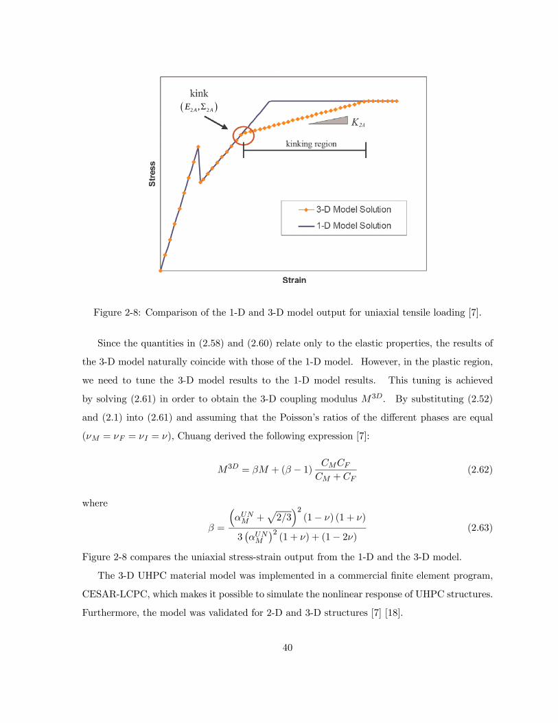
( )2 2,A AE Σ
Figure 2-8: Comparison of the 1-D and 3-D model output for uniaxial tensile loading [7].
Since the quantities in (2.58) and (2.60) relate only to the elastic properties, the results of
the 3-D model naturally coincide with those of the 1-D model. However, in the plastic region,
we need to tune the 3-D model results to the 1-D model results. This tuning is achieved
by solving (2.61) in order to obtain the 3-D coupling modulus M3D. By substituting (2.52)
and (2.1) into (2.61) and assuming that the Poisson’s ratios of the different phases are equal
(νM = νF = νI = ν), Chuang derived the following expression [7]:
M3D = βM + (β − 1) CMCF
CM + CF(2.62)
where
β =
³αUNM +
p2/3´2(1− ν) (1 + ν)
3¡αUNM
¢2(1 + ν) + (1− 2ν)
(2.63)
Figure 2-8 compares the uniaxial stress-strain output from the 1-D and the 3-D model.
The 3-D UHPC material model was implemented in a commercial finite element program,
CESAR-LCPC, which makes it possible to simulate the nonlinear response of UHPC structures.
Furthermore, the model was validated for 2-D and 3-D structures [7] [18].
40

2.4 Determination of Hardened Model Parameters
The two-phase UHPC model captures the overall composite behavior, at the macroscopic scale,
with a brittle-plastic matrix phase and an elasto-plastic fiber phase. Here, each phase is
considered as a macroscopic representation of the stiffness and the yield strength that are
added to obtain the stiffness and the strength of the overall UHPC composite. Due to the
macroscopic nature of the material model, all 3-D model parameters can be determined from
the macroscopic response of a UHPC material. The determination procedure of the model
parameters is achieved in the following way:
• Macroscopic material properties: The results of a tensile test and a compressive test are
used to identify the macroscopic stress-strain points of the idealized macroscopic stress-
strain response.
• Assumptions for the 3-D model parameters: Three simplifying assumptions are introduced
to reduce the number of model parameters of the isotropic UHPC material behavior.
• Determination of the 3-D model parameters: The 10 independent 3-D model parameters
are determined from the macroscopic stress-strain points.
2.4.1 Macroscopic Material Properties
UHPC materials can vary with the type of fibers a supplier chooses to use. The manufacturer
of DuctalTM (Lafarge) produces two types of UHPC material: one is DuctalTM -Steel Fiber,
and the other DuctalTM -Organic Fiber. DuctalTM -Steel Fiber was used in the test girders of
the Federal Highway Administration [FHWA] [7] and for the bridge girders optimized by MIT
for the FHWA [9]. The macroscopic material properties are obtained from a compression and
a tension test supplied by the manufacturer, which can be found in Reference [7]. One of the
tensile test results is shown in Figure 2-9. The macroscopic material properties of DuctalTM -
Steel Fiber that were extracted from this curve are summarized in Table 2.2. A simplified
stress-strain curve for the entire stress range is illustrated in Figure 2-10, with corresponding
strains presented in Table 2.3.
41

Figure 2-9: Average notch stress-displacement curve for DuctalTM -Steel Fiber [7].
Notation DuctalTM-SFMacroscopic K0 53.9 GPaStiffness K1 1.6 GPa
(≈ 3 % of K0)
Macroscopic Tension Σ−t,1 7.6 MPa
Strength Σ+t,1 6.9 MPa
Σt,2 11.5 MPaCompression Σ−c,1 190 MPa
Σ+c,1 173 MPa
Σc,2 183 MPa
Table 2.2: Macroscopic material properties of UHPC material and typical values for DuctalTM -Steel Fiber [18].
Tension CompressionInitial
Strain LimitEt,1 = 1.41× 10⁻⁴ Ec,1 = 3.40× 10⁻⁴
YieldStrain Limit
Et,2 = 3.02× 10⁻³ Ec,2 = 1.40× 10⁻²
Table 2.3: Macroscopic strain limits in the simplified stress-strain curve for DuctalTM -SteelFiber
42

,1tE ,2tE
,1t+Σ
,1t−Σ,2tΣ
E
Σ0K
1K
TENSION
,1cE,2cE
,1c+Σ
,1c−Σ
,2cΣ
COMPRESSION
Figure 2-10: Simplified stress-strain curve of UHPC in uniaxial tension and compression.
2.4.2 Review of the Assumptions for the 3-D Model Parameters
The isotropic UHPC material behavior is completely described by 15 material properties: 6
elastic properties (CM , νM , CF , νF , M3−D, and νI) and 9 strength properties (σMt, σMc,
σMb, σcrMt, σcrMc, σ
crMb, σFt, σFc, and σFb). In order to further reduce the number of model
parameters, three assumptions are introduced:
1. The Poisson’s ratio is the same in the matrix, the fiber, and the matrix-fiber coupling,
which makes νF and νI dependent parameters.
2. The post-cracking matrix strengths are reduced by the same factor, γcr defined by (2.19),
which makes σcrMc and σcrMb dependent parameters.
3. The loading function related to the biaxial compressive strength of the fiber is disregarded,
which makes σFb unnecessary.
These assumptions reduce the number of model parameters to 10 independent model pa-
rameters which can be obtained from the macroscopic stress-stain relationship. These model
parameters are summarized in Table 2.4.
43

2.4.3 Determination of the 3-D Model Parameters
Using (2.4) and (2.5), the six model parameters related to the tensile behavior of UHPC (CM ,
CF , M , σMt, σcrMt and σFt) are derived from the results of a tensile test.
In order to close the determination of the 3-D model parameters, we need to obtain the
four additional model parameters related to the compressive behavior and the Poisson’s ratio
of UHPC. The two model parameters related to the compressive behavior of UHPC (σMc and
σFc) are derived from the results of a uniaxial compression test using the following equations:
Σ−c,1 =³1 + CF
CM
´σMc ' σMc
Σ+c,1 = Σ−c,1 − CM
CM+M(σMc − σcrMc) ' σcrMc = γcrσMc
Σc,2 = σFc + σcrMc = σFc + γcrσMc
(2.64)
These equations have a form similar to the tensile strength relations in (2.2) and (2.5). The
composite matrix biaxial strength (σMb) can be determined from an additional test, a biaxial
compression test on an unreinforced cementitious specimen. More simply, it can be estimated
from known biaxial strength factors for unreinforced concrete as follows [11]:
σMb ≈ 1.2σMc (2.65)
Finally, the composite Poisson’s ratio (ν) can also be estimated from standard Poisson’s ratios
of cementitious materials:
ν = νM ≈ 0.17 (2.66)
In summary, the 3-D model parameters is obtained from a single tensile test and a single
compression test. Typical values for DuctalTM -Steel Fiber are summarized in Table 2.4. These
input model parameters are used throughout this report.
2.5 Chapter Summary
This chapter reviews the two-phase macroscopic model for the stress-strain behavior of hard-
ened UHPC material. A typical tensile response of hardened UHPC can be simplified in four
regions: an elastic behavior, a brittle strength drop, a post-cracking behavior, and a composite
44

Notation DuctalTM-SFElastic CM 53.9 GPaParameter CF 0.0 GPa
M 1.65 GPaν 0.17
Strength Matrix σMt (= ft + kM) 7.6 MPaParameter σcrMt (= kM) 6.9 MPa
σMc 190 MPaσMb 220 MPa
Fiber σFt (= fy) 4.6 MPaσFc 10 MPa
Table 2.4: Input material parameters of the 3D UHPC model and typical values DuctalTM -SteelFiber [18].
yielding. The 1-D model parameters properly capture the simplified UHPC material behavior
by introducing separately a composite matrix and a composite fiber phase. The 1-D hardened
UHPC model is easily extended to 3-D, by replacing the scalar quantities in the governing equa-
tions by their tensorial counterparts. The 3-D macroscopic model is constructed around three
main components: the 3-D constitutive relations, plasticity of the 3-D model, and consistency
with the 1-D model. The hardened 3-D UHPC model has the following interesting properties:
• The macroscopic nature of the two-phase model allows us to capture typical feature of
UHPC material behavior, with six material parameters of clear physical significance. The
stress drop modeled by this model allows the representation of progressive cracking with
increased loading. This makes it easy to fit the six material parameters of the model to
experimental test results.
• The two phase modeling of fibers and matrix allows a quantification of their individual
behaviors and their interaction. The cracking in UHPC is represented as permanent
plastic strains in the composite matrix, which allows one to evaluate the risk of cracking.
45

Chapter 3
HYDRATION KINETICS MODEL
FOR ORDINARY CONCRETE
The focus of the research presented here is the modeling of UHPC at early ages. Like for
all cement-based materials, the particular behavior of UHPC at early ages stems from the
hydration of cement, which is a highly exothermic and thermally activated reaction. The hy-
dration reaction leads to heat generation inducing thermal shrinkage during the cooling process.
Moreover, chemical shrinkage occurs because the volume of hydration products is less than the
original volume of cement and water. Concrete cracking at early ages is mainly caused by
both thermal and chemical shrinkage, which induce a severe state of stress beyond the mate-
rial strength developed. In this chapter, we review a hydration kinetics model for ordinary
concrete, which we extend in the sequel to UHPC materials.
3.1 Hydration of Cement
Ordinary Portland cement consists of various clinker phases, which react with water during
hydration. Most dominant clinker phases are1 tricalcium silicates (C3S), dicalcium silicates
(C2S), tricalcium aluminates (C3A) and tetracalcium aluminum ferrites (C4AF ). A typical
mineralogical composition and mass ratios of clinker phases in Portland cements are given in
1The notation of cement chemists is used; C = CaO; S = SiO2; A = Al2O3; F = Fe2O3; S = SO3;H = H2O.
46

Name ofCompound
OxideComposition
AbbreviationMass
Ratio [%]Tricalcium Silicates
(Alite)3CaO · SiO2 C3S 50-70
Dicalcium Silicates(Belite)
2CaO · SiO2 C2S 15-30
Tricalcium Aluminates(Aluminates)
3CaO ·Al2O3 C3A 5-10
Tetracalcium Aluminum Ferrites(Ferrites)
4CaO ·Al2O3 · Fe2O3 C4AF 5-15
Table 3.1: Main Compounds of Portland Cement [17].
Table 3.1. We describe briefly the hydration of silicates and aluminates, because the main
hydrates, which can be broadly classified as calcium silicate hydrates (C-S-H) and calcium
aluminate hydrates (C-A-H), form the most important part of the microstructure of a cement
paste. This section briefly reviews the simplified stoichiometric reactions for the hydration of
the four dominant compounds in Portland cement as suggested by Tennis and Jennings [23].
3.1.1 Silicate Hydration
The main products of the cement hydration are from the hydration of silicates, and they define
the quantity of calcium silicate hydrates (C-S-H) formed. The hydration reaction of C3S and
C2S can be written as follows:
2C3S + 10.6H → C3.4S2H8 + 2.6CH (3.1)
2C2S + 8.6H → C3.4S2H8 + 0.6CH (3.2)
In both cases, the products of the hydration are composed of calcium silicate hydrates (C-S-H)
and calcium hydroxide (CH). C-S-H constitutes approximately 50-70 % of the hydration
product volume, and its physical properties are of interest in connection with setting and
hardening properties of cement. CH, which is also called Portlandite, constitutes typically
20-25 % of the hydration product volume [10].
47

3.1.2 Aluminate Hydration
In the presence of sulfate (SO2−4 ) and water, C3A forms Ettringite (AFt phase):
C3A+ 3CSH2 + 26H → C6AS3H32 (3.3)
After the sulfate (SO2−4 ) is consumed, C3A and Ettringite (AFt phase) become monosulfoalu-
minates (AFm phase):
2C3A+ 3C6S3H32 + 4H → 3C6ASH12 (3.4)
After all the Ettringite (AFt) is consumed, the rest of C3A continues to hydrate as follows:
C3A+ CH + 12H → C4AH13 (3.5)
Many investigations have shown that the hydration of C4AF is very similar to that of C3A.
As in the case of C3A, the first crystalline products to form in the absence and presence of the
sulfate (SO−24 ) are AFm phase and AFt phase, respectively, and the AFt phase is later replaced
by AFm phase. Eventually, the product of the ferrite reaction is a hydrogarnet (C3 (A,F )H6)
described by the following equation:
C4AF + 2CH + 10H → 2C3 (A,F )H6 (3.6)
3.2 Macroscopic Modeling of Hydration Reaction for Ordinary
Concrete
As the hydration reaction progresses, the material stiffness increases, and the evolving stiffness
leads to the development of stresses in the material. The hydration reaction also affects the
strength of material, which influences the crack threshold at early age. Hence, there is a com-
petition between the stress development due to the evolving stiffness and the crack threshold
development due to strength growth. In order to capture the effects of thermal and chemi-
cal phenomena related to hydration reaction on the mechanical properties, a thermodynamic
framework is necessary for the modeling. This section reviews the thermo-chemo-mechanical
48

modeling of the hydration reaction proposed by Ulm and Coussy [25] [26].
3.2.1 Simplification of Hydration Reaction Modeling
Given the complexity of the hydration of cement as presented in Section 3.1, it is useful to
simplify the different process in a first engineering approach. Ulm and Coussy suggest the
diffusion of water through the layers of hydrates as the dominant mechanism of the hydration
kinetics2. For the reaction to occur, water diffuses through the layers of hydrates. Once water
meets the unhydrated cement, new hydrates are formed instantaneously compared to the time
scale of the diffusion process. Figure 3-1 illustrates this hydration reaction process, and the
hydration reaction can be simplified as follows:
Free Water → Combined Water (3.7)
where the reactant phase corresponds to the free water and the product phase to the water
combined in the hydrates. Furthermore, as a measure of the reaction extent, a hydration
degree (ξ) is introduced and it is defined by the following equation:
ξ (t) =m (t)
m∞(3.8)
where m∞ is the asymptotic value of combined water mass, and m (t) is the combined water
mass at time t. At the beginning of the reaction, the hydration degree is zero. As the hydration
progresses, it increases. Eventually, the hydration degree becomes one when the reaction is
complete. The hydration degree is controlled by the chemical affinity A, which represents
the thermodynamic imbalance between the chemical potentials of reactant phase and product
phase.
2Kinetics is the branch of chemistry that is concerned with the rates of change in the concentration of reactantsin a chemical reaction.
49

Figure 3-1: Diffusion of water through layers of hydrates [25].
3.2.2 Thermodynamic Framework for Ordinary Concrete at Early Ages
Like the hardened 3-D UHPC model, the starting point of the hydration kinetics model is the
Clausius-Duhem inequality3 [24]:
ϕdt = Σ : dE− SdT − dΨ ≥ 0 (3.9)
where ϕdt stands for the dissipation; Σ and E are the 2nd order macroscopic stress tensor and
macroscopic strain tensor, respectively; S and T stand for the entropy and absolute temperature,
respectively; and Ψ is the free energy. Assuming the elementary system to be closed, the
hydration degree, ξ (t), can be considered as an internal state variable. For concrete at early
ages, there are three state variables, E, T and ξ , which describe the energy state of the system.
In the framework of physical linearization, the free energy is limited to a 2nd order expansion
with respect to external state variables, E and T , and it reads:
Ψ = Ψ (ε, T, ξ) (3.10)
= Ψ0 +Ψ2 +Ψ1
3The Clausius-Duhem inequality states that the external energy supplied in form of work is not entirely storedin the system in form of elastic energy that can be recovered later on; but dissipated into heat form.
50

where Ψ0 is the free energy relating to the initial state of stress, entropy, and chemical affinity;
Ψ2 relates to the elastic potential energy which is a second-order tensor expansion with respect
to strain, absolute temperature and hydration degree; and Ψ1 is the free energy associated with
the coupling of phenomena of different origins:
Ψ0 = Σ0 : E− S0 (T − T0)−A0ξ
Ψ2 =12E : C (ξ) : E−
12CT0(T − T0)
2 + 12κξ
2
Ψ1 = −C (ξ) : E : α (T − T0)− C (ξ) : E : βξ + LT0ξ (T − T0)
(3.11)
where subscript "0" means initial state of each driving force; C (ξ) is the 4th order stiffness
tensors of the aging concrete; C is the volume heat capacity; κ is a coefficient relating to the
hydration kinetics; α is the 2nd order thermal dilatation coefficient tensor; β is the 2nd order
chemical dilatation coefficient tensor; and L is the latent heat of the hydration reaction. Here,
for the sake of simplicity, the thermal and chemical dilatation coefficient tensors (α and β)
are constant, and the volume heat capacity, the hydration kinetics coefficient and the latent
heat (C, κ and L) are also considered to be constant. Use of (3.10) in (3.9) yields the state
equations, which read in an incremental form:
⎧⎪⎪⎪⎨⎪⎪⎪⎩dΣ
dS
dA
⎫⎪⎪⎪⎬⎪⎪⎪⎭ =
⎡⎢⎢⎢⎣C (ξ) −C (ξ) : α −C (ξ) : β
C (ξ) : α CT0
− LT0
C (ξ) : β − LT0
−κ
⎤⎥⎥⎥⎦ :⎧⎪⎪⎪⎨⎪⎪⎪⎩
dE
dT
dξ
⎫⎪⎪⎪⎬⎪⎪⎪⎭ (3.12)
where the hypothesis of infinitesimal deformation is applied so that each driving force can be
expressed by only the terms of the same order of magnitude as strain. In this derivation, the
strains due to elastic, thermal, and chemical change are infinitesimal:
trε¿ 1
trεt = tr (α (T − T0))¿ 1
trεc = tr (βξ)¿ 1
(3.13)
where εt and εc denote the strains due to thermal change and chemical change, respectively.
It is generally found that the thermal changes and chemical changes affect the mechanical
51
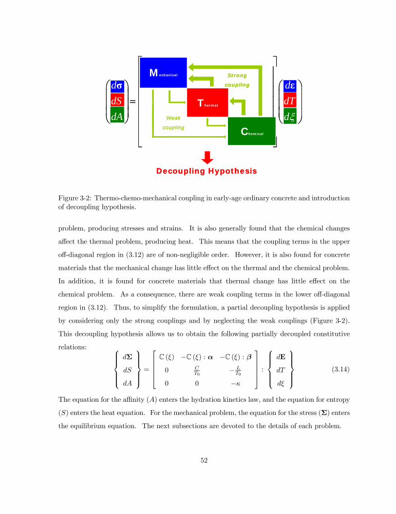
0
0
( ) - ( ) : - ( ) :
( ) : - -
( ) : - -
d dC LdS dTT T
dA dLT
ξ ξ α ξ β
ξ αξ
ξ β κ
⎡ ⎤⎢ ⎥⎢ ⎥⎛ ⎞ ⎛ ⎞⎢ ⎥⎜ ⎟ ⎜ ⎟= ⎢ ⎥⎜ ⎟ ⎜ ⎟⎢ ⎥⎜ ⎟ ⎜ ⎟
⎝ ⎠ ⎝ ⎠⎢ ⎥⎢ ⎥⎣ ⎦
C C Cσ ε
C
CWeak
coupling
Strong
coupling
Decoupling Hypothesis
Mechanical
Thermal
Chemical
0
0
( ) - ( ) : - ( ) :
( ) : - -
( ) : - -
d dC LdS dTT T
dA dLT
ξ ξ α ξ β
ξ αξ
ξ β κ
⎡ ⎤⎢ ⎥⎢ ⎥⎛ ⎞ ⎛ ⎞⎢ ⎥⎜ ⎟ ⎜ ⎟= ⎢ ⎥⎜ ⎟ ⎜ ⎟⎢ ⎥⎜ ⎟ ⎜ ⎟
⎝ ⎠ ⎝ ⎠⎢ ⎥⎢ ⎥⎣ ⎦
C C Cσ ε
C
CWeak
coupling
Strong
coupling
Decoupling Hypothesis
Mechanical
Thermal
Chemical
Figure 3-2: Thermo-chemo-mechanical coupling in early-age ordinary concrete and introductionof decoupling hypothesis.
problem, producing stresses and strains. It is also generally found that the chemical changes
affect the thermal problem, producing heat. This means that the coupling terms in the upper
off-diagonal region in (3.12) are of non-negligible order. However, it is also found for concrete
materials that the mechanical change has little effect on the thermal and the chemical problem.
In addition, it is found for concrete materials that thermal change has little effect on the
chemical problem. As a consequence, there are weak coupling terms in the lower off-diagonal
region in (3.12). Thus, to simplify the formulation, a partial decoupling hypothesis is applied
by considering only the strong couplings and by neglecting the weak couplings (Figure 3-2).
This decoupling hypothesis allows us to obtain the following partially decoupled constitutive
relations: ⎧⎪⎪⎪⎨⎪⎪⎪⎩dΣ
dS
dA
⎫⎪⎪⎪⎬⎪⎪⎪⎭ =
⎡⎢⎢⎢⎣C (ξ) −C (ξ) : α −C (ξ) : β
0 CT0
− LT0
0 0 −κ
⎤⎥⎥⎥⎦ :⎧⎪⎪⎪⎨⎪⎪⎪⎩
dE
dT
dξ
⎫⎪⎪⎪⎬⎪⎪⎪⎭ (3.14)
The equation for the affinity (A) enters the hydration kinetics law, and the equation for entropy
(S) enters the heat equation. For the mechanical problem, the equation for the stress (Σ) enters
the equilibrium equation. The next subsections are devoted to the details of each problem.
52

Hydration Kinetics
From the partially decoupled constitutive relations (3.14), the affinity is given by:
dA = −κdξ (3.15)
If we integrate both sides of the equation, it is readily found that the affinity which depends on
the hydration degree:
A = A (ξ) (3.16)
The form of A (ξ) specifies the reaction order. It is the driving force of the reaction kinetics.
This reaction kinetics is specified by a kinetics law, which for a thermally activated chemical
reaction reads:
dξ
dt=
A (ξ)
τ∗ (T0)exp
∙−Ea
R
µ1
T− 1
T0
¶¸(3.17)
=A (ξ)
τ (T0)exp
∙− Ea
RT
¸
where
τ (T0) = τ∗ (T0) exp
∙− Ea
RT
¸(3.18)
Here, τ∗ and τ are the characteristic reaction times4; Ea is the activation energy of the hy-
dration reaction5; and R is the universal gas constant. The value of Ea/R can be found in
cement chemistry handbooks [13]. Once known, the chemical affinity, A (ξ), can be obtained
from experiments which allow us to access the hydration reaction rate, dξ/dt, and the charac-
teristic reaction time, τ . The experiments can be one of adiabatic calorimetric experiments or
isothermal strength evolution tests as detailed below.
4The characteristic time (τ∗ or τ) depends typically on the type of cement.5The activation energy over the universal gas constant (Ea/R) is a constant for most cement and is known
to be roughly 4, 000 K.
53

Heat Equation
From the partially decoupled constitutive relations (3.14), the equation for entropy can be
written as follows:
dS =C
T0dT − L
T0dξ (3.19)
This entropy expression enters the 2nd law of thermodynamics of the closed system reading:
T0dS
dt− ϕ = −divq (3.20)
where ϕ is the dissipation rate, divq is the external rate of heat supply to the elementary system
provided by conduction, and q is the heat flux vector. For the heat condition, a linear law is
adopted reading:
q = −K·∇T = −K∇T (3.21)
where K = K1 is the thermal conductivity tensor in the isotropic case. The thermal con-
ductivity, K, might depend on the hydration degree, but it is assumed to be constant in this
model.
Assuming that the latent heat due to deformation and the heat due to chemical dissipation
are negligible with respect to the latent hydration heat L, substituting (3.19) and (3.21) into
(3.20) yields the following heat equation:
CdT
dt= K∇2T + L
dξ
dt(3.22)
where the left side of the equation, C dT/dt, means change in energy stored within the system,
the first term on the right side, K∇2T , is the net heat rate provided from the outside by
conduction, and the term, L dξ/dt, is the heat generated by hydration. Thus, this heat
equation states that the stored energy change due to the temperature variation is equal to
the sum of the external heat supply due to thermal conductivity and the latent heat of the
hydration reaction.
The heat equation needs to be completed by thermal boundary conditions, which prescribe
54

either the temperature or the heat flux through the boundary, ∂Ω:
T = T d on ∂ΩT
q · n = qd on ∂Ωq
q · n = λ (T − Text) on ∂Ωλ
(3.23)
∂ΩT ∪ ∂Ωq ∪ ∂Ωλ = ∂Ω
∂ΩT ∩ ∂Ωq = ∂Ωq ∩ ∂Ωλ = ∂Ωλ ∩ ∂ΩT = 0(3.24)
where n is the normal unit vector toward the outside of ∂Ωq or ∂Ωλ; T d and qd are the
prescribed temperature and the heat flux, respectively; λ is the exchange coefficient6; and Text
is the external temperature. Solving simultaneously the heat equation (3.22) and the hydration
kinetics law (3.17) for the boundary conditions (3.23) allows one to determine a materials or
structural system.
Equilibrium Equation
From (3.14), the constitutive equation for stress reads:
dΣ = C (ξ) : dE− C (ξ) : αdT −C (ξ) : βdξ (3.25)
Three effects relative to early-age concrete behavior are considered in (3.25):
• The aging elasticity, C (ξ), representing the increase of the stiffness as a function of the
hydration degree;
• The thermal stresses, −C (ξ) : αdT , related to restrained thermal dilatation;
• The chemical stresses, −C (ξ) : βdξ, related to restrained autogenous shrinkage.
The general 3-D constitutive model involves 39 (= 21 + 2× 9) parameters associated with
the stiffness tensor C (ξ) , the thermal dilatation coefficient tensor α, and the chemical dilatation
6The exchange coefficients for various external conditions can be found in Reference [27].
55

tensor β. In the isotropic case, the stiffness tensor can be described by two unique scalar values:
C (ξ) = 3K (ξ)K+2G (ξ) J (3.26)
where K (ξ) is the aging bulk modulus, and G (ξ) is the aging shear modulus of concrete. The
aging bulk modulus and the aging shear modulus are related to the aging Young’s modulus of
the concrete, E (ξ), by:
K (ξ) = E(ξ)3(1−2ν)
G (ξ) = E(ξ)2(1+ν)
(3.27)
where ν is the Poisson’s ratios of the concrete. The Poisson’s ratio is assumed to be constant
in the modeling. Isotropy of the material also implies:
α=α1; β = β1 (3.28)
where α and β are the thermal and the chemical dilatation coefficient, respectively. Equation
(3.25) can be restated in an isotropic format:
dΣ = dΣv1+ dΣd (3.29)
where dΣv = 13 tr (dΣ) is the volumetric stress increment; and dΣd is the deviatoric stress
increment. The volumetric stress-strains are represented by:
dΣv = 3K (ξ) (dEv − αdT − βdξ) (3.30)
where dEv = 13tr (dE) is the volumetric strain increment. Similarly, the deviatoric stress-strain
relations are given by:
dΣd = 2G (ξ) dEd (3.31)
where dEd = dE− dEv1 is deviatoric strain increment.
The constitutive relations are complete by applying the results of the hydration kinetics
and the heat equation, i.e. the time history of the temperature and the hydration degree in the
system. With this constitutive relation , the stress equilibrium equation is solved in order to
56

find statically admissible stress fields:
divΣ+ ρf = 0
where ρ is the mass density; and f is the volume force density.
3.3 Macroscopic Investigation of Hydration Kinetics for Ordi-
nary Concrete
As shown in Section 3.2.2, the hydration kinetics is the starting point of modeling ordinary
concrete at early ages. Thus, the determination of the chemical affinity function, A (ξ), plays
an important role in the modeling. In order to determine experimentally the chemical affinity
expressed in (3.17), the evolution of the hydration degree, ξ(t), and the time history of tem-
perature, T (ξ), must be measured. Here, two generally accepted experiments are reviewed;
adiabatic calorimetry experiment and isothermal strength evolution.
3.3.1 Adiabatic Calorimetric Experiment
The adiabatic calorimetric experiment is a standard method for accessing hydration kinetics.
It is generally admitted that the increase rate of adiabatic temperature is proportional to the
hydration reaction rate as follows:dξ
dt∝ dT ad
dt(3.32)
where T ad is the adiabatic temperature. Writing the heat equation (3.22) for adiabatic condi-
tions (divq = 0) yields after integration:
ξ (t) =T ad (t)− T ad
0
L/C(3.33)
57

where L/C = T ad∞ − T ad
0 is the adiabatic temperature rise; and T ad0 and T ad
∞ are the initial and
the final temperatures in the experiment. Then, writing (3.33) in the kinetic law (3.17) yields:
dξ
dt=
1
T ad∞ − T0
dT ad
dt(3.34)
=A (ξ)
τ¡T ad0
¢exp ∙− Ea
RT ad (t)
¸
Eventually, the normalized chemical affinity, A (ξ), is identified from the adiabatic calorimetric
experiment:
A (ξ) =A (ξ)
τ¡T ad0
¢ (3.35)
= exp
∙Ea
RT ad (t)
¸1
T ad∞ − T ad
0
dT ad
dt
Ulm and Coussy [26] suggested that A (ξ) was an intrinsic kinetic function; i.e. on that does
not depends on boundary conditions.
3.3.2 Isothermal Strength Evolution
The strength growth is another manifestation of the hydration reaction. It is generally admitted
that the increase rate of isothermal strength growth is proportional to the hydration rate:
dξ
dt∝ df iso
dt(3.36)
where f iso is the isothermal strength value. Similarly to (3.33), the hydration degree is deter-
mined from strength measurements:
ξ (t) =f iso (t)− f0fad∞ − f0
(3.37)
where f iso0 (≤ 0) is a reference strength value for ξ = 0, which relates to the percolation thresh-
old; and fad∞ is the asymptotic strength at complete hydration. Then, using (3.37) in (3.17)
58
yields a second means to a access the hydration rate from:
dξ
dt=
1
f iso∞ − f0
df iso
dt(3.38)
=A (ξ)
τ¡T iso0
¢exp ∙− Ea
RT iso0
¸
Eventually, the normalized chemical affinity, A (ξ), is identified from the isothermal strength
evolution test:
A (ξ) =A (ξ)
τ¡T iso0
¢ (3.39)
= exp
∙Ea
RT iso0
¸1
f iso∞ − f0
df iso
dt
3.4 Chapter Summary
In this chapter, we reviewed a hydration kinetics model for ordinary concrete, which allows the
modeling of thermo-chemo-mechanical couplings of concrete at early ages at the macro-level of
material description. The main points to be noted are:
• The diffusion of free water through the layers of hydrates is considered as the dominant
mechanism of the hydration with respect to the kinetics. The model for ordinary con-
crete at early ages accounts explicitly for the hydration reaction at the macroscopic scale
through the hydration degree ξ.
• By means of some simplifying decoupling hypothesis, it is possible to obtain partially de-
coupled constitutive relations which are easy to handle: hydration kinetics, heat equation
and stress constitutive equation.
• In this model, the normalized affinity A considered to be an intrinsic kinetic function,
which characterizes the macroscopic hydration kinetics of concrete. This function can be
determined from standard material tests, such as calorimetric tests or material strength
evolution tests.
59

Part II
MATERIAL MODELING
60

Chapter 4
EARLY-AGE UHPC MATERIAL
MODEL
This Chapter is dedicated to the development of a new material model for early-age UHPC,
which combines the hardened UHPC model reviewed in Chapter 2 and the hydration kinetics
model reviewed in Chapter 3. We start by considering the additional features we consider
in the modeling of early-age UHPC behavior. The model is then developed in a consistent
thermodynamic framework, and consistent decoupling hypothesis are introduced to obtain an
appropriate engineering model for the prediction of temperature, stresses and strains in early-
age UHPC.
4.1 Evolving UHPC Material Model
Unlike hardened UHPC, the properties of UHPC at early ages are not constant, but evolve
as the hydration progresses. In terms of the 1-D Think model of UHPC, displayed in Figure
4-1 (a), the strength and stiffness properties relating to the matrix phase now depend on the
hydration degree:
CM → CM (ξ)
ft → ft (ξ)
kM → kM (ξ)
(4.1)
61

(a) (b)
Matrix stress
( ),1t ξ+Σ
( ),1t ξ−Σ( ) ( )t Mf kξ ξ+
( ),2t ξΣ
E
Σ
Fiber stress
( )0K ξ ( )1K ξ
( ) ( )F yfσ ξ ξ=
( ) ( )M Mkσ ξ ξ=
Matrix stress
( ),1t ξ+Σ
( ),1t ξ−Σ( ) ( )t Mf kξ ξ+
( ),2t ξΣ
E
Σ
Fiber stress
( )0K ξ ( )1K ξ
( ) ( )F yfσ ξ ξ=
( ) ( )M Mkσ ξ ξ=
CFC
M
M
CC
M
kft(ξ)
CM(ξ) kM(ξ)
M(ξ)fy(ξ)
CFC
M
M
CC
M
kft(ξ)
CM(ξ) kM(ξ)
M(ξ)fy(ξ)
E
pMε
pFε
M Fσ σΣ = +
CFC
M
M
CC
M
kft(ξ)
CM(ξ) kM(ξ)
M(ξ)fy(ξ)
CFC
M
M
CC
M
kft(ξ)
CM(ξ) kM(ξ)
M(ξ)fy(ξ)
E
pMε
pFε
M Fσ σΣ = +
Figure 4-1: (a) 1-D Think Model of a two-phase matrix-fiber composite material for UHPC atearly-ages, (b) Stress-strain response for UHPC at early ages.
Furthermore, since the composite fiber phase in the 1-D model represents the plastic pullout
behavior of the fibers during composite yielding (see Section 2.2), it is readily understood that
this pullout behavior also depends on the hydration state of the matrix phase:
fy → fy (ξ) (4.2)
Similarly, the coupling modulus M , which links the irreversible matrix behavior (plastic strain
εpM) with the irreversible reinforcing fiber behavior (plastic strain εpF ), is also affected by the
hydration state of the matrix phase. This is expressed by considering the coupling modulus
M as a function of the hydration degree:
M →M (ξ) (4.3)
These modifications regarding the stiffness and strength parameters of the 1-D UHPC model
are depicted in Figure 4-1 (a).
62

Like in the case of the hardened UHPC model, the following relations between macroscopic
material properties and model parameters are obtained (see Figure 4-1 (b)):
K0 (ξ) ' CM (ξ)
K1 (ξ) ' CM (ξ)M(ξ)CM (ξ)+M(ξ)
(4.4)
Σ−t,1 (ξ) ' ft (ξ) + kM (ξ) with E−1 =ft(ξ)+kM (ξ)
CM (ξ)
Σ+t,1 (ξ) ' kM (ξ) with E+1 =ft(ξ)+kM (ξ)
CM (ξ)
Σt,2 (ξ) = fy (ξ) + kM (ξ) with E2 ' kM (ξ)M(ξ)+fy(ξ)[CM (ξ)+M(ξ)]CM (ξ)M(ξ)
(4.5)
The mechanical properties (compressive strength, tensile strength, and modulus of elastic-
ity) all increase as functions of the hydration degree. The stiffness and strength properties are
zero prior to the percolation of the solid matrix phase, and evolve to their asymptotic values
which correspond to the values of the hardened UHPC material. In between these two as-
ymptotes, an interpolation is necessary. Unfortunately, there has been little research on the
evolution of strength and stiffness for UHPC. In a first approach, we will adopt interpolation
laws developed for ordinary concrete to UHPC, namely Laube’s law for strength growth and
Byfors’ law for stiffness.
4.1.1 Evolution of Strength
It is often found, for ordinary concrete materials [3], that the tensile strength at early ages grows
faster than the compressive strength. However, Bernard et al. [4] showed that this effect was
due to the presence of large aggregates activating friction in compression (but not in tension).
Since UHPC have no large aggregates, it is appropriate, therefore, to adopt one single evolution
law for both tensile and compressive strength. As a first engineering approximation for the
strength parameters in the UHPC model we adopt a linear relationship known as Laube’s Law
[14]. If a strength is denoted by f (ξ), Laube’s law has the following form:
f (ξ) = f∞kf (ξ) (4.6)
63

Evolution of Strength & Stiffness
0.0
0.2
0.4
0.6
0.8
1.0
0.0 0.2 0.4 0.6 0.8 1.0
Hydration Degree [1]
Rela
tive V
alu
es [
1] 1
Strength
Stiffness
Setting =
Percolation Threshold
Byfor’s Law
Laube’s Law
100 % Hydration
Evolution of Strength & Stiffness
0.0
0.2
0.4
0.6
0.8
1.0
0.0 0.2 0.4 0.6 0.8 1.0
Hydration Degree [1]
Rela
tive V
alu
es [
1] 1
Strength
Stiffness
Setting =
Percolation Threshold
Byfor’s Law
Laube’s Law
100 % Hydration
Figure 4-2: Evolution of strength and stiffness adopted in the modeling of UHPC at early-ages.
where f∞ is the strength of the hardened material, and kf (ξ) is the aging factor for strength.
The aging factor reads:
kf (ξ) =
⎧⎨⎩ξ010ξ if ξ ≤ ξ01− ξ0
101−ξ0 (ξ − ξ0) +
ξ010 if ξ > ξ0
(4.7)
where ξ0 stands for the percolation threshold. Solid diamonds in Figure 4-2 illustrate Laube’s
law which we adopt for the strength growth of UHPC at early ages. Significant strength starts
to develop only after setting1.
4.1.2 Evolution of Stiffness
It is generally agreed that Young’s modulus increases faster than the compressive and tensile
strength [3]. This is due to the change of morphology of the hydration products. This
1 It should be noted that the non-zero value of the strength below the percolation threshold is introduced forstability reason only.
64

difference between stiffness and strength development is a manifestation of early-age cracking
sensitivity, because the generated stress depends on the Young’s modulus, whereas the resistance
to cracking depends on the tensile strength.
Inspired by developments for ordinary concrete, a nonlinear relationship known as Byfors’
law [6] is adopted for the stiffness growth of the UHPC model. If a stiffness is denoted by
C (ξ) , Byfors’ law has the following form:
C (ξ) = C∞kc (ξ) (4.8)
where C∞ is the Young’s modulus of the hardened material, and kc (ξ) is the aging factor for
the stiffness. The aging factor reads:
kc (ξ) =1 + 1.37 [Rc∞]
2.204
1 + 1.37 [Rc (ξ)]2.204
∙Rc (ξ)
Rc∞
¸2.675(4.9)
where Rc∞ is the compressive strength of the hardened material [unit: MPa], and Rc (ξ) is the
compressive strength of the aging material as a function of the hydration degree ξ. A bilinear
relation is introduced for Rc (ξ) as follows:
Rc (ξ) =
⎧⎨⎩ ξRc0 if ξ ≤ ξ0Rc∞−Rc01−ξ0
(ξ − ξ0) +Rc0 if ξ > ξ0
(4.10)
where ξ0 is the threshold of the hardened material and Rc0 =110ξ0Rc∞. Hollow squares in
Figure 4-2 illustrate the adopted evolution law for the stiffness of UHPC at early ages. It is
worthwhile to note that significant mechanical properties start to develop only after setting.
4.2 Thermodynamic Framework for UHPC at Early Ages
In the previous section, we introduced some ad-hoc modification to the hardened UHPCmaterial
model. At this stage of the development, a closer look on the thermodynamic consistency of
the model is in order.
65

4.2.1 Free Energy and State Equations
Like for the hardened 3-D UHPC (see Section 2.3.1) and the hydration kinetics model (see
Section 3.2.2), the starting point of our modeling is the Clausius-Duhem inequality [24]:
ϕdt = Σ : dE− SdT − dΨ ≥ 0 (4.11)
where ϕdt stands for the dissipation; Σ and E are the 2nd order macroscopic stress tensor and
macroscopic strain tensor, respectively; S and T stand for the entropy and absolute temperature,
respectively; and Ψ is the free energy. Like in the early-age model for ordinary concrete (see
Chapter 3), assuming the elementary system as closed, the hydration degree, ξ (t), is considered
as an internal state variables [25] [26]. For UHPC at early ages, however, there are five state
variables, E, εpM , εpF , T and ξ , which describe the energy state of the system. The free energy
is assumed of the form:
Ψ = Ψ¡E− εpM ,E− εpF , ε
pM − ε
pF , T, ξ
¢(4.12)
= Ψ0 +Ψ2 +Ψ1
where:
Ψ0 = σM,0 :¡E− εpM
¢+ σF,0 :
¡E− εpF
¢− S0 (T − T0)−A0ξ (4.13)
Ψ2 =12
£E− εpM
¤: CM (ξ) :
£E− εpM
¤+ 1
2
£E− εpF
¤: CF (ξ) :
£E− εpF
¤+12
£εpM − ε
pF
¤: M (ξ) :
£εpM − ε
pF
¤− 1
2CT0(T − T0)
2 − 12κξ
2
Ψ1 = −CM (ξ) :£E− εpM
¤: αM (T − T0)− CF (ξ) :
£E− εpF
¤: αF (T − T0)
−CM (ξ) :£E− εpM
¤: βMξ − CF (ξ) :
£E− εpF
¤: βF ξ +
LT0ξ (T − T0)
In (4.13), subscript "0" means initial state of each driving force; σM and σF stand for the stress
of the composite matrix and the composite fiber, respectively2; CM (ξ), CF (ξ) and M (ξ) are
the 4th order stiffness tensors of the composite matrix, the composite fiber, and the matrix-fiber
2The sum of the matrix stress and the fiber stress is always equal to the macroscopic stress, which holds aswell for the initial state of stress:
Σ0 = σM,0 + σF,0
66

coupling; C is the volume heat capacity; κ is a coefficient relating to the hydration kinetics;
αM and αF are the 2nd order thermal dilatation coefficient tensors of the composite matrix
and the composite fiber; βM and βF are the 2nd order chemical dilatation coefficient tensors
of the composite matrix and the composite fiber; and L is the latent heat of the hydration
reaction. In a first-order engineering approach, the thermal and chemical dilatation coefficient
tensors (αM , αF , βM and βF ) are considered to be constant, and the volume heat capacity,
the hydration kinetics coefficient and the latent heat (C, κ and L) as well. Use of (4.12) in
(4.11) yields the Clausius-Duhem inequality in the form:
ϕdt = σM : dεpM + σF : dεpF +Adξ ≥ 0 (4.14)
together with the state equations:
Σ =∂Ψ
∂E(4.15)
= Σ0 +CM (ξ) :£E− εpM
¤+CF :
£E− εpF
¤− [CM (ξ) : αM +CF : αF ] (T − T0)
− [CM (ξ) : βM +CF : βF ] ξ
σM = − ∂Ψ
∂εpM(4.16)
= σM,0 +CM (ξ) :£E− εpM
¤−M (ξ) :
£εpM − ε
pF
¤−CM (ξ) : αM (T − T0)− CM (ξ) : βMξ
σF = − ∂Ψ
∂εpF(4.17)
= σF,0 +CF :£E− εpF
¤+M (ξ) :
£εpM − ε
pF
¤−CF : αF (T − T0)−CF : βF ξ
67

S = −∂Ψ∂T
(4.18)
= S0 +C
T0(T − T0)−
L
T0ξ
+CM (ξ) :£E− εpM
¤: αM +CF :
£E− εpF
¤: αF
A = −∂Ψ∂ξ
(4.19)
= S0 − κξ − L
T0(T − T0)
+CM (ξ) :£E− εpM
¤: βM +CF :
£E− εpF
¤: βF
From (4.14) to (4.19), we identify σM , σF and A as the thermodynamic driving forces associated
with the dissipation of the energy caused by dεpM , dεpF and dξ, respectively.
4.2.2 Maxwell Symmetries and Decoupling Hypothesis
One key feature of the thermodynamic approach is that it allows one to account and work out
the couplings (or thermodynamic cross-effects) between phenomena of different origin through
the Maxwell symmetries that come from the choice of the free energy expression (4.13). These
are:
• The coupling between the different stress quantities (Σ, σM and σF ) which characterize
the UHPC material model (see Section 2.3.1):
CM (ξ) = − ∂Σ∂εpM
= ∂σM∂E
CF = − ∂Σ∂εpF
= ∂σF∂E
M (ξ) = ∂σM∂εpF
= ∂σF∂εpM
(4.20)
• The coupling between the stresses (Σ, σM and σF ) and the entropy (S) which relate to
thermal dilatation and latent deformation heat effects:
αMCM (ξ) +αFCF = −∂Σ∂T =
∂S∂E
αMCM (ξ) = −∂σM∂T = − ∂S
∂εpM
αFCF = −∂σF∂T = − ∂S
∂εpF
(4.21)
68

• The coupling between the stresses (Σ, σM and σF ) and the chemical affinity (A) which
relate to chemical dilatation (or shrinkage) and stress induced phase change phenomena:
βMCM (ξ) + βFCF = −∂Σ∂ξ =
∂A∂E
βMCM (ξ) = −∂σM∂ξ = − ∂A
∂εpM
βFCF = −∂σF∂ξ = − ∂A
∂εpF
(4.22)
• The coupling between the entropy (S) and the chemical affinity (A) which relate to the
latent heat of hydration and temperature induced phase change phenomena:
L
T0= −∂A
∂T= −∂S
∂ξ(4.23)
Using these notations, we obtain the following system of equations:
⎧⎪⎪⎪⎪⎪⎪⎪⎪⎪⎨⎪⎪⎪⎪⎪⎪⎪⎪⎪⎩
dΣ
dσM
dσF
dS
dA
⎫⎪⎪⎪⎪⎪⎪⎪⎪⎪⎬⎪⎪⎪⎪⎪⎪⎪⎪⎪⎭= [K1] :
⎧⎪⎪⎪⎪⎪⎪⎨⎪⎪⎪⎪⎪⎪⎩
dE− dεpM
dE− dεpF
dT
dξ
⎫⎪⎪⎪⎪⎪⎪⎬⎪⎪⎪⎪⎪⎪⎭(4.24)
where:
[K1] =
⎡⎢⎢⎢⎢⎢⎢⎢⎢⎢⎢⎢⎢⎣
CM (ξ) CF
*−CM (ξ) :αM
−CF :αF
+ *−CM (ξ) :βM
−CF :βF
+CM (ξ)+M (ξ) −M (ξ) −CM (ξ) :αM −CM (ξ) :βM
−M (ξ) CF+M (ξ) −CF :αF −CF :βF
CM (ξ) :αM CF :αF C/T 0 −L/T 0CM (ξ) :βM CF :βF −L/T 0 κ
⎤⎥⎥⎥⎥⎥⎥⎥⎥⎥⎥⎥⎥⎦(4.25)
We note that these relations are such that at any time,
dΣ = dσM + dσF (4.26)
69

0 0
0
( ) ( ): : ( ): :( ) ( ) ( ) ( ): ( ):
( ) ( ) : :1 ( )( ): :
1 ( )( ): :
M F M M F F M M F F
M M M M M
M F F F F F
FM M F F
M M F F
dd
dd C F
T TdSdA F
T
ξ ξ ξξ ξ ξ ξ ξ
ξ ξξξξ
ξξ κξ
⎡ ⎤⎢ ⎥⎛ ⎞ ⎢ ⎥⎜ ⎟ ⎢ ⎥⎜ ⎟ ⎢ ⎥⎜ ⎟=⎢ ⎥⎜ ⎟ ⎢ ⎥⎜ ⎟ ⎢
− − − −+ − − −
⎥⎜ ⎟⎝ ⎠ ⎢ ⎥
⎢ ⎥⎣
− + − −∂
−∂
−∂ ⎦
∂−
C C C α C α C β C βΣ C M M C α C β
Εσ M C M C α C βσ
C α C α
C β C β
pMpF
dd d
dTdξ
⎛ ⎞⎜ ⎟⎜ ⎟⎜ ⎟⎜ ⎟⎜ ⎟⎝ ⎠
−−ε
Ε ε
weak coupling
strong coupling
Decoupling Hypothesis
Mechanical
Thermal
Chemical
Figure 4-3: Thermo-chemo-mechanical coupling in early-age UHPC and introduction of decou-pling hypothesis.
Like for ordinary concrete, some of these couplings are rather weak, while others are strong.
In a first engineering approach, we consider only the strong coupling terms, which are situated
in the upper off-diagonal region in (4.24). Thermal and chemical changes produce stresses
or strains, and the chemical changes produces heat. On the other hand, the coupling terms
in the lower off-diagonal region in (4.24) are considered to be weak, because, for concrete
materials, the mechanical change has little effect on the thermal and the chemical problem,
and the thermal change has little effect on the chemical problem in precipitation reactions.
Figure 4-3 illustrates how the decoupling hypothesis is applied to the constitutive relations.
Introducing the decoupling hypothesis in (4.24) allows us to obtain the following partially
decoupled constitutive relations:
⎧⎪⎪⎪⎪⎪⎪⎪⎪⎪⎨⎪⎪⎪⎪⎪⎪⎪⎪⎪⎩
dΣ
dσM
dσF
dS
dA
⎫⎪⎪⎪⎪⎪⎪⎪⎪⎪⎬⎪⎪⎪⎪⎪⎪⎪⎪⎪⎭= [K2] :
⎧⎪⎪⎪⎪⎪⎪⎨⎪⎪⎪⎪⎪⎪⎩
dE− dεpM
dE− dεpF
dT
dξ
⎫⎪⎪⎪⎪⎪⎪⎬⎪⎪⎪⎪⎪⎪⎭(4.27)
70

where:
[K2] =
⎡⎢⎢⎢⎢⎢⎢⎢⎢⎢⎢⎢⎢⎣
CM (ξ) CF
*−CM (ξ) :αM
−CF :αF
+ *−CM (ξ) :βM
−CF :βF
+CM (ξ)+M (ξ) −M (ξ) −CM (ξ) :αM −CM (ξ) :βM
−M (ξ) CF+M (ξ) −CF :αF −CF :βF
0 0 C/T 0 −L/T 00 0 0 κ
⎤⎥⎥⎥⎥⎥⎥⎥⎥⎥⎥⎥⎥⎦(4.28)
Thus, the equation for affinity A, which enters the hydration kinetics law, depends only on
the hydration degree. The equation for entropy S, which enters the heat equation for the
thermal problem, depends only on temperature and hydration degree. Only the equations for
the stresses (Σ, σM and σF ) depend on all state variables. This will turn out to be the key
to the evaluation of the risk of early-age UHPC cracking.
4.2.3 Hydration Kinetics and Heat
Thanks to the decoupling hypothesis, the kinetics of the hydration and the equation of the
entropy for the modeling of UHPC early ages have the same form as the ones for ordinary
concrete, i.e. (3.15) and (3.19) in Section 3.2.2:
dA = −κdξ ⇒ A = A (ξ) (4.29)
dS =C
T0dT − L
T0dξ (4.30)
Thus, all derivations relating to the thermal and chemical problem for ordinary concrete can be
equally applied to the modeling of UHPC at early ages. For instance, the hydration kinetics
law reads:dξ
dt=
A (ξ)
τ (T0)exp
∙− Ea
RT
¸(4.31)
and the heat equation reads:
CdT
dt= k∇2T + L
dξ
dt(4.32)
In order to complete the macroscopic modeling for UHPC at early ages, we need to perform
71
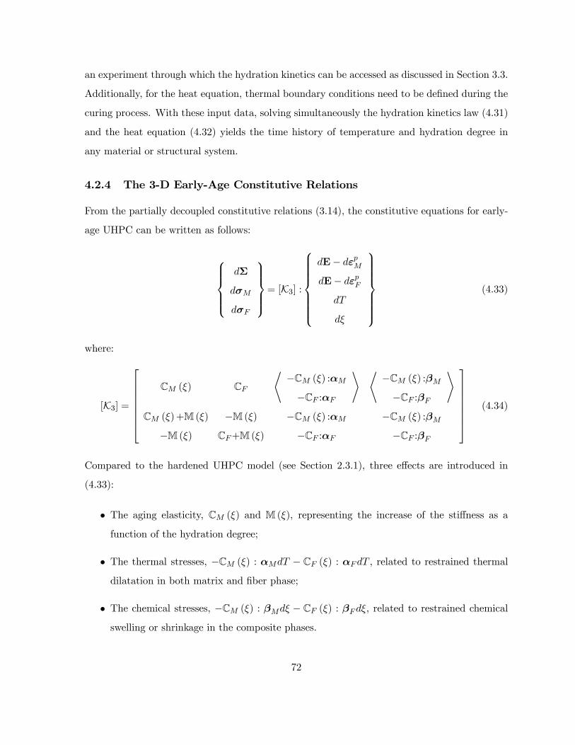
an experiment through which the hydration kinetics can be accessed as discussed in Section 3.3.
Additionally, for the heat equation, thermal boundary conditions need to be defined during the
curing process. With these input data, solving simultaneously the hydration kinetics law (4.31)
and the heat equation (4.32) yields the time history of temperature and hydration degree in
any material or structural system.
4.2.4 The 3-D Early-Age Constitutive Relations
From the partially decoupled constitutive relations (3.14), the constitutive equations for early-
age UHPC can be written as follows:
⎧⎪⎪⎪⎨⎪⎪⎪⎩dΣ
dσM
dσF
⎫⎪⎪⎪⎬⎪⎪⎪⎭= [K3] :⎧⎪⎪⎪⎪⎪⎪⎨⎪⎪⎪⎪⎪⎪⎩
dE− dεpM
dE− dεpF
dT
dξ
⎫⎪⎪⎪⎪⎪⎪⎬⎪⎪⎪⎪⎪⎪⎭(4.33)
where:
[K3] =
⎡⎢⎢⎢⎢⎢⎢⎣CM (ξ) CF
*−CM (ξ) :αM
−CF :αF
+ *−CM (ξ) :βM
−CF :βF
+CM (ξ)+M (ξ) −M (ξ) −CM (ξ) :αM −CM (ξ) :βM
−M (ξ) CF+M (ξ) −CF :αF −CF :βF
⎤⎥⎥⎥⎥⎥⎥⎦ (4.34)
Compared to the hardened UHPC model (see Section 2.3.1), three effects are introduced in
(4.33):
• The aging elasticity, CM (ξ) and M (ξ), representing the increase of the stiffness as a
function of the hydration degree;
• The thermal stresses, −CM (ξ) : αMdT − CF (ξ) : αFdT , related to restrained thermal
dilatation in both matrix and fiber phase;
• The chemical stresses, −CM (ξ) : βMdξ − CF (ξ) : βFdξ, related to restrained chemical
swelling or shrinkage in the composite phases.
72

The general 3-D constitutive model involves 99 (= 3 × 21 + 4 × 9) parameters associated
with the evolving stiffness tensors (CM (ξ), CF and M (ξ)), the thermal dilatation coefficient
tensors (αM and αF ), and the chemical dilatation tensor (βM and βF ). In the isotropic case,
the stiffness tensors can be reduced to:
CM (ξ) = 3KM (ξ)K+2GM (ξ) J
CF = 3KFK+2GFJ
M (ξ) = 3KI (ξ)K+2GI (ξ) J
(4.35)
where KM (ξ), KF and KI (ξ) are the bulk moduli of the composite matrix, the composite
fiber and the matrix-fiber coupling, respectively; GM (ξ), GF and GI (ξ) are the evolving shear
moduli of the composite matrix, the composite fiber and the matrix-fiber coupling, respectively.
The bulk moduli and the shear moduli are related to the elastic moduli of the composite matrix,
CM (ξ), the composite fiber, CF , and matrix-fiber coupling, M (ξ), by:
KM (ξ) =CM (ξ)
3(1−2νM ) ; GM (ξ) =CM (ξ)2(1+νM )
;
KF =CF
3(1−2νF ) ; GF =CF
2(1+νF );
KI (ξ) =M3D(ξ)3(1−2νI) ; GI =
M3D(ξ)2(1+νI)
(4.36)
where νM , νF and νI are the Poisson’s ratios of the the composite matrix, the composite fiber
and the matrix-fiber coupling, respectively; and M3D (ξ) is the 3-D counterpart3 of M (ξ) in
the 1-D model (see Figure 4-1). The Poisson’s ratios are assumed to be constant in the model.
Moreover, the isotropy of the material implies:
αM=αM1; αF=αF1;
βM = βM1; βF = βF1(4.37)
where αM and βM are the thermal and the chemical dilatation coefficient of the composite
matrix, respectively; and αF and βF are the thermal and the chemical dilatation coefficient of
the composite fiber, respectively.
3Unlike the composite matrix stiffness and the composite fiber stiffness, the 3-D coupling stiffness tensorM (ξ)is not directly related to its 1-D counter partM . The 3-D coupling stiffness tensor must be formulated in such away that the 3-D model gives the same macroscopic uniaxial response as the 1-D model, as explained in Section2.3.3.
73
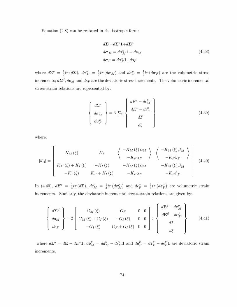
Equation (2.8) can be restated in the isotropic form:
dΣ =dΣv1+dΣd
dσM = dσvM1+ dsM
dσF = dσvF1+dsF
(4.38)
where dΣv = 13tr (dΣ), dσ
vM = 1
3 tr (dσM) and dσvF = 13tr (dσF ) are the volumetric stress
increments; dΣd, dsM and dsF are the deviatoric stress increments. The volumetric incremental
stress-strain relations are represented by:
⎧⎪⎪⎪⎨⎪⎪⎪⎩dΣv
dσvM
dσvF
⎫⎪⎪⎪⎬⎪⎪⎪⎭ = 3 [K4]
⎧⎪⎪⎪⎪⎪⎪⎨⎪⎪⎪⎪⎪⎪⎩
dEv − d pM
dEv − d pF
dT
dξ
⎫⎪⎪⎪⎪⎪⎪⎬⎪⎪⎪⎪⎪⎪⎭(4.39)
where:
[K4] =
⎡⎢⎢⎢⎢⎢⎢⎣KM (ξ) KF
*−KM (ξ)αM
−KFαF
+ *−KM (ξ)βM
−KFβF
+KM (ξ) +KI (ξ) −KI (ξ) −KM (ξ)αM −KM (ξ)βM
−KI (ξ) KF +KI (ξ) −KFαF −KFβF
⎤⎥⎥⎥⎥⎥⎥⎦ (4.40)
In (4.40), dEv = 13tr (dE), d
pM = 1
3 tr¡dεpM
¢and d p
F = 13tr¡dεpF
¢are volumetric strain
increments. Similarly, the deviatoric incremental stress-strain relations are given by:
⎧⎪⎪⎪⎨⎪⎪⎪⎩dΣd
dsM
dsF
⎫⎪⎪⎪⎬⎪⎪⎪⎭ = 2
⎡⎢⎢⎢⎣GM (ξ) GF 0 0
GM (ξ) +GI (ξ) −GI (ξ) 0 0
−GI (ξ) GF +GI (ξ) 0 0
⎤⎥⎥⎥⎦ :⎧⎪⎪⎪⎪⎪⎪⎨⎪⎪⎪⎪⎪⎪⎩
dEd − depM
dEd − depF
dT
dξ
⎫⎪⎪⎪⎪⎪⎪⎬⎪⎪⎪⎪⎪⎪⎭(4.41)
where dEd = dE − dEv1, depM = dεpM − d pM1 and depF = dεpF − d p
F1 are deviatoric strain
increments.
74

The constitutive relations (4.39) and (4.41) require as input the time history of the tem-
perature and the hydration degree in the system. With this constitutive relations, the stress
equilibrium equation is solved in order to find statically admissible stress fields:
divΣ+ ρf = 0 (4.42)
4.2.5 Plasticity of the 3-D Early-Age Model
In order to establish the plastic behavior of the 3-D early-age UHPC model, 3-D loading func-
tions and flow rules need to be constructed.
The 3-D Early-Age Strength Domain
The 3-D strength domain for UHPC at early ages is very similar to that of the hardened UHPC
model. In fact, the only difference is that the strength properties of UHPC are now a function
of the hydration degree: the 3-D strength domain evolves. Like in the hardened UHPC model
(see Section 2.3.2), the early-age UHPC strength domain is also characterized by 6 macroscopic
strength values (Σ−t,1 (ξ), Σ−c,1 (ξ), Σ
−b,1 (ξ), Σt,2 (ξ), Σc,2 (ξ) and Σb,2 (ξ)), which now evolve as the
hydration progresses. The evolution of the strength properties are assumed to follow Laube’s
law explained in Section 4.1.1.
From a modeling point of view, the strength domain DE of UHPC, which is described by
the 3-D loading function F , is governed by the individual behaviors of the composite matrix
and the composite fiber (2.15):
Σ (ξ) ∈ DE ⇔ F = max [FM , FF ] ≤ 0 ⇔*σM (ξ) ∈ DM ⇔ FM (σM , ξ) ≤ 0
σF (ξ) ∈ DF ⇔ FF (σF , ξ) ≤ 0
+(4.43)
where the 3-D loading functions (FM and FF ) are dependent on the hydration degree. More
precisely, the 3-D loading function of the composite matrix, FM , is captured by three higher
initial limits (σMt (ξ), σMc (ξ) and σMb (ξ)) and three lower yield limits (σcrMt (ξ), σcrMc (ξ) and
σcrMb (ξ)). For early-age UHPC, we can describe the strength domain of the composite matrix
75

as follows:
σM (ξ) ∈ DM ⇔
FM (σM , ξ) =
*F 0M = max
hfTC,0M , fUN,0
M , fBI,0M
ibefore cracking
F crM = max
hfTC,crM , fUN,cr
M , fBI,crM
iafter cracking
+≤ 0
(4.44)
wherefTC,0M = I1,M (ξ)− σMt (ξ) ≤ 0
fUN,0M = αUNM (ξ) I1,M (ξ) + |sM (ξ)|− cUN,0
M (ξ) ≤ 0
fBI,0M = αBIM (ξ) I1,M (ξ) + |sM (ξ)|− cBI,0M (ξ) ≤ 0
(4.45)
fTC,crM = I1,M (ξ)− σcrMt (ξ) ≤ 0
fUN,crM = αUNM (ξ) I1,M (ξ) + |sM (ξ)|− cUN,cr
M (ξ) ≤ 0
fBI,crM = αBIM (ξ) I1,M (ξ) + |sM (ξ)|− cBI,crM (ξ) ≤ 0
(4.46)
where the friction coefficients (αi) and the cohesion (ci) is still defined by (2.18) and (2.21);
except for their dependence on the hydration degree.
Furthermore, the 3-D loading function of the composite fiber, FF , is captured by three
characteristic values, i.e. σFt (ξ), σFc (ξ) and σFb (ξ). For early-age UHPC, the strength
domain of the composite fiber is described as follows:
σF (ξ) ∈ DF ⇔ FF (σF , ξ) = max£fTCF , fDP
F
¤≤ 0 (4.47)
wherefTCF = I1,F (ξ)− σFt (ξ) ≤ 0
fDPF = αUNF (ξ) I (ξ)1,F + |sF (ξ)|− cDP
F (ξ) ≤ 0(4.48)
The 3-D Early-Age Plastic Flow Rule
The composite matrix and composite fiber are both governed by the following Kuhn-Tucker
conditions:
FM (σM , ξ) ≤ 0; dλM ≥ 0; FM (σM , ξ) dλM = 0 (4.49)
FF (σF , ξ) ≤ 0; dλF ≥ 0; FF (σF , ξ) dλF = 0 (4.50)
76

where dλM and dλF are the plastic multipliers that represent the intensity of the plastic flow in
the composite matrix and the composite fiber, respectively. Like in the hardened 3-D UHPC
model, an associated plastic flow rule is adopted for the 3-D early-age UHPC model. Hence,
using (2.29), the permanent deformations of the composite matrix and the composite fiber read:
dεpM =Xi
dλM,i∂FM,i (σM , ξ)
∂σM(4.51)
= dλTCM 1+ dλUNM£αUNM 1+NsM (ξ)
¤+ dλBIM
£αBIM 1+NsM (ξ)
¤
dεpF =Xi
dλF,i (ξ)∂FF,i (σF , ξ)
∂σF(4.52)
= dλTCF 1+ dλDPF
£αUNF 1+NsF (ξ)
¤where the loading functions of the composite matrix are still defined in Table 2.1; NsM = sM
|sM |
and NsF =sF|sF | are the normalized deviatoric stress tensor of the composite matrix and the
composite fiber, respectively.
4.2.6 Consistency with the 1-D Model
In a last step of our constitutive developments, we need to ensure the consistency of the 3-D
model with the 1-D model response. By introducing the same Poisson’s ratio for all components
(νM = νF = νI ≡ ν) in the 3-D model and assuming the Poisson’s ratio does not change during
hydration, the consistency with the 1-D model is ensured by the following 3-D coupling modulus:
M3D (ξ) = β (ξ)M (ξ) + [β (ξ)− 1] CM (ξ)CF
CM (ξ) + CF(4.53)
where
β (ξ) =
hαUNM (ξ) +
p2/3i2(1− ν) (1 + ν)
3£αUNM (ξ)
¤2(1 + ν) + (1− 2ν)
(4.54)
Like other stiffness values, the evolution of the coupling modulus is assumed to follow Byfors’
Law (see Section 4.1.2).
Based on the reasoning explored in Section 2.3.3, a uniaxial stress-strain output from the
77

3-D early-age UHPC model can now be obtained with the hydration degree as parameter. The
noteworthy four stress-strain points in the Exx − Σxx curve are functions of the hydration
degree: ³Exx,1 (ξ) , Σ
−xx,1 (ξ)
´= (Exx, Σxx)|Σxx(ξ)=σMt(ξ), Σyy(ξ)=0
(4.55)³Exx,1 (ξ) , Σ
+xx,1 (ξ)
´=³Exx|Σxx(ξ)=σMt(ξ), Σyy(ξ)=0
, Σxx|Σxx=σcrMt(ξ)
´(4.56)
(Exx,2A (ξ) , Σxx,2A (ξ)) = (Exx, Σxx)|Σyy(ξ)=0, fUN,crM (ξ)=0, fTCF (ξ)=0(4.57)
(Exx,2B (ξ) , Σxx,2 (ξ)) = (Exx, Σxx)| Σyy=0, fTC,crM (ξ)=0,
fUN,crM (ξ)=0, fTCF (ξ)=0
(4.58)
=
⎛⎝Exx|Σyy(ξ)=0, fTC,crM (ξ)=0,
fUN,crM (ξ)=0, fTCF (ξ)=0
, Σxx|Σxx(ξ)=σcrMt(ξ)+σFt(ξ)
⎞⎠Following the procedure used to derive (2.38)-(2.49) for hardened UHPC, the above equations
lead to an analytical solution for the four points. Similarly, the evolving stiffness is obtained
analytically:
K0 (ξ) =∂Σxx∂Exx
¯Σyy(ξ)=0
(4.59)
K1 (ξ) =∂Σxx∂Exx
¯Σyy(ξ)=0, fUNM (ξ)=0
(4.60)
K2A (ξ) =∂Σxx∂Exx
¯Σyy(ξ)=0, fUNM (ξ)=0, fTCF (ξ)=0
(4.61)
These three stiffness values for the early-age UHPC model can be computed using a similar
approach as the one employed to derive (2.50)-(2.57) for the hardened UHPC model.
Figure 4-4 displays the analytical solutions for different hydration degrees4. We can clearly
see the evolution of the stiffness and strength as the hydration progresses. These analytical
results will be used later on for verification purposes of the model implementation in a finite
element environment.
4The material properties of DuctalTM -Steel Fiber are used for the model parameters of the hardened UHPCmaterial, as listed in Table 2.4. In order to see the evolution of the material properties, four cases of hydrationdegree are considered, i.e. ξ = 0.25, 0.5, 0.75 and 1.0.
78

Analytical Solutions
0
4
8
12
0 2 4 6 8 10
Strain [1/1000]
Str
ess
[MP
a]
xi=1.0xi=0.75xi=0.5xi=0.25
Analytical Solutions
0
2
4
6
8
0.0 0.1 0.2 0.3
Strain [1/1000]
Str
ess
[MP
a]
xi=1.0xi=0.75xi=0.5xi=0.25
(a)
(b)
Figure 4-4: Uniaxial stress-strain behavior obtained from the analytical solution: (a) Entirestress-strain curve, (b) Focus on first cracking behavior.
79

4.3 Chapter Summary
The thermo-chemo-mechanical coupling model of UHPC is the combination of the two-phase
mechanical model of hardened UHPC and the thermo-chemo-mechanical coupling model for
ordinary early-age concrete. The coupling of these two model is achieved by considering
the evolution of the strength and stiffness properties in the two-phase UHPC material model.
As a first engineering approach, a linear evolution law [Laube’s law] is adopted for strength,
and stiffness is assumed to follow a nonlinear evolution law [Byfors’ law]. The couplings
[thermodynamic cross-effects] between phenomena of different origin are investigated through
the Maxwell symmetries that come from the choice of the free energy expression. Like in
the ordinary concrete constitutive relations, it is assumed that the thermodynamic imbalance
induced by stress, temperature and plastic evolutions are negligible for the hydration reaction.
Finally, The 3-D macroscopic model for UHPC at early ages is constructed in three steps:
• Determination of the 3-D constitutive relations: The 3-D stress-strain relations are ob-
tained using thermodynamic approach.
• Determination of strength domain and plastic deformation of the 3-D model: The 3-
D strength limits evolve as the hydration progresses. Thus, the 3-D loading functions
depend on the hydration degree. Like for the hardened UHPC model, an associated
plastic flow rule is adopted.
• Consistency of the 3-D model with the 1-D model: The 3-D model is designed to give
consistent results with the 1-D model; and this over the entire hydration process.
80

Chapter 5
FINITE ELEMENT
IMPLEMENTATION
The finite element implementation of the early-age UHPC model represents the link between
material modeling and structural application. With the finite element implementation of the
early-age UHPC model, one can simulate structural behavior composed of UHPC at early
ages. In this Chapter, the finite element formulation and the realization of the model is
discussed. While the thermo-chemical model does not differ much from the one available for
ordinary concrete, and is implemented in several finite element programs, the contribution of
this research is formulation and implementation of the thermo-chemo-mechanical model. This
chapter presents details on the finite element implementation of the early-age UHPC model in
a commercial finite element program, CESAR-LCPC. Moreover, in order to verify the newly
implemented module, uniaxial responses of an early-age UHPC element are compared with the
analytical solutions developed in Chapter 4.
5.1 Finite Element Formulation
Thanks to the decoupling hypothesis, the simulations can be carried out in a two-step manner.
First, the thermo-chemical problem is solved. The results are used as input in the thermo-
chemo-mechanical problem to determine deflection, stress, etc.
81

5.1.1 Principle of Virtual Displacements
The mechanical finite element analysis problem for early-age UHPC can be stated as follows:
Given
⎧⎪⎪⎪⎪⎪⎪⎪⎪⎪⎨⎪⎪⎪⎪⎪⎪⎪⎪⎪⎩
Geometry of Body
Force Boundary Condition: fd and Td
Displacement Boundary Condition: ξd
Material Stress-strain Law
Temperature and Hydration Degree History: T (x, t) and ξ (x, t)
Calculate
⎧⎪⎪⎪⎨⎪⎪⎪⎩Displacements: ξ
The Corresponding Strains: E, εpM and εpF
The Corresponding Stress: Σ, σM and σF
where f is the volume force density; T is the surface force density; ξ is the displacement; the
superscript "d" indicate the prescribed quantities; and Σ and E are the macroscopic stress and
strain tensor, respectively1. In order to close the above boundary value problem, the following
three conditions must be satisfied:
• Stress Equilibrium:
divΣ+ ρf = 0 (5.1)
where ρ is the mass density. In the case of the UHPC model, it should be noted that
only the macroscopic stress Σ enters the stress equilibrium equation. By contrast, the
values of the stresses in the individual components (σM and σF ) are dictated by their
state equations (4.33).
• Geometrical Compatibility (strain-displacement relation):
E =1
2
¡gradξ + gradξT
¢(5.2)
1Dimensions of the quantities are followings:
[f ] = FM−1 = LT−2; [T] = FL−2 =ML−1T−2
82

This equation can be obtained from the infinitesimal deformation assumption.
• Material Law (constitutive relation and plastic evolution law):
Σ = Σ (E, ...) (5.3)
For the early-age UHPC, the constitutive relation is given by (4.33), and the plastic
evolution law by (4.43).
The basis of the displacement-based finite element solution is the principle of virtual dis-
placements. This principle states that the total internal virtual work be equal to the total
external virtual work, for any compatible small virtual displacements imposed on the system.
The principle reads [2]:
Wint =
ZΩE : ΣdΩ (5.4)
=
ZΩξ · ρfdΩ+
Z∂Ωξ ·Tda = Wext
where Wint and Wext are the internal and external virtual work, respectively; ξ is the virtual
displacement; and E is the corresponding virtual strain (the over-bar denoting virtual quanti-
ties). The equation in the first row represents the virtual work of the internal stress, and the
equation in the second row expresses the virtual work done by the external forces (volume and
surface forces).
5.1.2 Finite Element Equations
Finite element analysis requires the spacial discretization of the system to be analyzed. The
entire system is approximated as an assemblage of discrete finite elements inter-connected at
nodal points on the element boundaries. For an element k, the displacement field ξk (x) is
assumed to be a function of the unknown global displacements at the nodes U:
ξk (x) =hNkiU (5.5)
83

where£Nk¤is the displacement interpolation matrix for the element k, and the superscript "k"
denotes the element number2. The choice of element and the construction of the corresponding
entries in£Nk¤constitute the basic steps of a finite element solution. From the assumption
of the displacement field in (5.5), the corresponding macroscopic strain for the element k is
expressed by:
Ek (x) =hBkiU (5.6)
where£Bk (x)
¤is the strain-displacement matrix3 for the element k.
For the use of the principle of virtual displacements, the same assumptions are applied to
the virtual displacements and the macroscopic strains for element k:
ξk=hNki ©
Uª
(5.7)
Ek =hBki ©
Uª
(5.8)
2Here, we express symmetric 2nd and 4th order tensors in matrix form. For example, the 2nd order straintensor (3× 3) is expressed in a 6× 1 vector form:
E =
⎡⎣ Exx Exy Exz
Exy Eyy Eyz
Exz Eyz Ezz
⎤⎦ → E = Exx Eyy Ezz Exy Exz EyzT
By adopting this notation, we can express the following quantities in matrix form:
ξ⇒ n× 1; Nk ⇒ n×m; U⇒ m× 1
where n is the dimension of the problem, and m is the total number of degree of freedom of the consideredelement.
3The strain-displacement matrix for the element k is given by:
Bk (x) =Nk (x)
dx
By adopting the condensed matrix notation for symmetric tensors, we express the following quantities inmatrix form:
E⇒ 2n× 1; Bk ⇒ 2n×m
where n is the dimension of the problem, and m is the total number of degree of freedom of the consideredelement.
84

Substitution of the previous relations into (5.4) yields:
Wint =Xk
ZΩk
©UªT h
BkiTΣkdΩk (5.9)
=Xk
ZΩk
©UªT h
NkiT
ρfkdΩk +Xk
Z∂Ωk
©UªT h
NkiTTkd
³∂Ωk
´= Wext
By introducing new notations for internal and external forces at the nodes (Fint and Fext),
this equation can be simplified as follows:
Wint =©UªT Fint = ©UªT Fext = Wext (5.10)
whereFint =
Xk
RΩk
£Bk¤TΣkdΩk
Fext =Xk
RΩk
£Nk¤T
ρfkdΩk +Xk
R∂Ωk
£Nk¤TTkd
¡∂Ωk
¢ (5.11)
Since (5.10) must hold for any value of the virtual displacement©UªT , we obtain:
R = Fext− Fint = 0 (5.12)
where R is the residual force vector for the global force equilibrium.
For a nonlinear material law, an iteration procedure is required to solve the above equation
until the residual force vector is close to zero. In this study, the Newton-Raphson method is
adopted:
nF(i)int
o=
nF(i−1)int
o+
∂nF(i−1)int
o∂©U (i)
ª n∆U (i)
o(5.13)
=nF(i−1)int
o+
*Xk
ZΩk
hBkiT µ∂Σ
∂E
¶k,(i) hBkidΩk
+n∆U (i)
o=
nF(i−1)int
o+hK(i) (ξ)
in∆U (i)
owhere (i) is the number of the iteration step in the Newton-Raphson method; ∆U (i) = U (i) −
U (i−1) is the corresponding incremental residual displacement; and£K(i) (ξ)
¤is the correspond-
85

ing stiffness matrix of the element assemblage which is now a function of the eventually spatially
varying hydration degree. From (5.12) and (5.13), the unknown incremental residual displace-
ments©∆U (i)
ªare calculated at each iteration using the residual force vector
©R(i−1)
ª:
hK(i) (ξ)
in∆U (i)
o= Fext−
nF(i−1)int
o=nR(i−1)
o(5.14)
Based on this iteration scheme, the unknown displacement U can be obtained for a nonlinear
material law.
The iteration procedure, however, is not necessary for elastic behavior. From (4.33),¡∂Σ∂E
¢k,(i)is equal to the sum of the 4th order stiffness tensors for the composite matrix and
the composite fiber: µ∂Σ
∂E
¶k,(i)
= CkM
³ξk´+Ck
F (5.15)
Thus,©∆U (i)
ªcan be easily obtained for elastic behavior from (5.14), using the following
explicit equation of£K(i) (ξ)
¤:
hK(i) (ξ)
i=Xk
ZΩk
hBkiT D
CkM
³ξk´+Ck
F
EhBk (x)
idΩk (5.16)
Following the previously described iteration scheme, the unknown displacement U =©∆U (1)
ªis obtained at the first iteration step for elastic behavior4.
Solving the finite element equation for plastic behavior requires some special care to obtain
the stiffness matrix£K(i) (ξ)
¤and the internal nodal force at nodes
nF(i)int
o. First, it is not
as straightforward to obtain£K(i) (ξ)
¤for plastic behavior as it is for linear elastic behavior,
because it requires to calculate a tangent operator between two consecutive iterative stress
states. Generally, there are two ways to obtain¡∂Σ∂E
¢k,(i): one is to use the initial tangent
operator, i.e. (5.15), and the other is to use consistent tangent operators [22]. In this study the
former method is used for simplicity of the formulation. Furthermore, in order to calculate the
4At the first iteratation step (i = 1), the internal force at the nodes is zero:
F(0)int = 0
86

internal forcenF(i)int
oat nodes according to (5.11), the plastically admissible macroscopic stress
Σk,(i) is required. These stresses are calculated in an iterative fashion from the infinitesimal
state equation (4.33) written in an incremental form:
Σk,(i) = Σk,(i−1) (5.17)
+CkM
³ξk´:h∆Ek,(i) −∆εp,k,(i)M
i+Ck
F :h∆Ek,(i) −∆εp,k,(i)F
i−hCkM
³ξk´: αk
M +CkF : α
kF
i∆T k −
hCkM
³ξk´: βk
M +CkF : β
kF
i∆ξk
where ∆Ek,(i) =£Bk¤ ©∆U (i)
ª; ∆T k and ∆ξk are obtained at each time step from the thermo-
chemical finite element analysis; and ∆εp,k,(i−1)M and ∆εp,k,(i−1)M can be obtained from a return
mapping algorithm. This return mapping algorithm is discussed in the following section.
5.1.3 Return Mapping Algorithm
An implicit backward Euler difference scheme is adopted as the return mapping algorithm
in order to obtain the plastically admissible macroscopic stress Σ for a given set of material
parameters and strain history. The return mapping algorithm applies the state and evolution
equations of the constitutive model in a spatially discretized form through an iterative procedure
[22]. With this procedure, the two-phase and multi-loading surface problem of early-age UHPC
reduces to the standard problem of finding the closest distance of the trial stress state to the
elastic domain. Within a finite element procedure, this algorithm discretizes the constitutive
models at the level of the integration points.
The implementation of the 3-D early-age UHPC model requires us to consider simulta-
neously the five different loading surfaces5 given by (4.44) and (4.47). The return mapping
algorithm presented in this section applies to the general 3-D case. However, this method is
5Before cracking, the five loading functions are:
fTC,0M , fUN,0M and fBI,0M for the composite matrixfTCF and fDPF for the composite fiber
After cracking, those are:
fTC,crM , fUN,crM and fBI,crM for the composite matrixfTCF and fDPF for the composite fiber
87

easily adapted for uniaxial, biaxial and plane stress condition; and Reference [7] provides details
of these conditions.
Before entering the details of the return mapping algorithm, we summarize the quantities
that are given as input for the algorithm. These are:
• The thermo-chemical state variables (T k and ξk) and their incremental values (∆T k and
∆ξk) which are obtained from the thermo-chemical finite element analysis at each time
step, and each point in the structure.
• The incremental displacement ∆U (i) which is obtained from the (modified) Newton-
Raphson scheme:
hK(0) (ξ)
in∆U (i)
o= Fext−
nF(i−1)int
o=nR(i−1)
o(5.18)
where£K(0) (ξ)
¤is the elastic stiffness matrix of the element assemblage calculated at
the beginning of each time step (during the time step iterations the hydration does not
evolve).
• The incremental macroscopic strain which is calculated from the given incremental resid-
ual displacement; analogous to (5.6):
∆Ek,(i) =hBkin∆U (i)
o(5.19)
Strictly speaking, all state variables of the system and the cracking variable have to include a
superscript (i) for the iteration number of the Newton-Raphson scheme. Furthermore, another
superscript k for elements has to be included. However, they are omitted for simplicity of the
notation in this section. This is because the whole return mapping algorithm is carried out
at the integration point of each element and for each iteration of the Newton-Raphson scheme,
and notations are repetitive. The following simplified notation will be used:
∆T k ⇒ ∆T ; ∆ξk ⇒ ∆ξ; ∆Ek,(i) ⇒ ∆E; (5.20)
88

Σk,(i−1) ⇒ Σin; σk,(i−1)M ⇒ σM,in; σ
k,(i−1)F ⇒ σM,in;
Ek,(i−1) ⇒ Ein; εp,k,(i−1)M ⇒ εpM,in; ε
p,k,(i−1)F ⇒ εpF,in; χk,(i−1) ⇒ χin
(5.21)
Σk,(i) ⇒ Σout; σk,(i)M ⇒ σM,out; σ
k,(i)F ⇒ σM,out;
Ek,(i) ⇒ Eout; εp,k,(i)M ⇒ εpM,out; ε
p,k,(i)F ⇒ εpF,out; χk,(i) ⇒ χout
(5.22)
where the subscript "in" indicates the input quantities, which correspond to a plastically ad-
missible stress field of the previous Newton-Raphson iteration (i− 1) before considering the
incremental macroscopic strain ∆E; and the the subscript "out" indicates the output quanti-
ties, which correspond to a plastically admissible stress field of the current Newton-Raphson
iteration (i) after considering the incremental macroscopic strain ∆E.
The 3-D return mapping algorithm assumes that the rest of the thermodynamic state vari-
ables of the system (E − εpM and E − εpF ) and a cracking state variable (χ) are also known
inputs of the return mapping algorithm:
¡E− εpM , E− εpF , χ
¢|in =
³Ein − εpM,in, Ein − εpF,in, χin
´where the cracking state variable indicates the cracking condition in the composite matrix. It
is defined as follows:
χin = Y¡¯εpM¯¢
(5.23)
where¯εpM¯is the magnitude of the plastic strain tensor of the composite matrix; and Y (xh)
is the Heaviside function defined by:
Y (xh) =
⎧⎨⎩ 0 if xh ≤ 0
1 if xh > 0(5.24)
Here, only two composite matrix cracking states are modeled: χ = 0 if the composite matrix
has not cracked, χ = 1 if the composite matrix has cracked.
Given the incremental values of the thermodynamic state variables (∆T and ∆ξ), the return
mapping algorithm provides the updated state variables and cracking variable:
¡E− εpM , E− εpF , χ
¢|out =
³Eout − εpM,out, Eout − εpF,out, χout
´
89

Thus, the 3-D early-age UHPC constitutive equations and plastic evolution equations are dis-
cretized with respect to iteration steps of the Newton-Raphson method. Based on these
discretized constitutive relations, the return mapping algorithm can be broken down in the
following four steps:
1. Compute trial values.
2. Check yield conditions. If F ≤ 0, go to Step 4. Otherwise, proceed to Step 3.
3. Solve for the plastic strains. Then, go to Step 2.
4. Update the stresses.
The 3-D early-age UHPCmodel may require multiple iterations checking the yield conditions
(Step 2) and solving the plastic strains (Step 3).
Step 1: Compute Trial Values.
We first assume that the imposed incremental macroscopic strain ∆E affects the stresses elasti-
cally. Then, the trial stresses in the composite matrix and in the composite fiber are calculated
from (4.38)-(4.41) in an incremental fashion:
σM,tr = σM,in + 3KM [∆Ev − αM∆T − βM∆ξ]1+ 2GM∆E
d
σF,tr = σF,in + 3KF [∆Ev − αF∆T − βF∆ξ]1+ 2GF∆E
d(5.25)
The trial stresses (σM,tr and σF,tr) are not guaranteed to be plastically admissible. These
trial stresses are calculated from the stresses of the previous step (σM,in and σF,in) for given
incremental values of the thermodynamic state variables (∆T and ∆ξ) and the incremental
macroscopic strain (∆E).
As a first step, these elastically assumed trial stresses are temporarily considered as the
updated solutions:
σM,up = σM,tr; σF,up = σF,tr (5.26)
where the subscript "up" indicates the updated quantities. Based on this elastic assumption,
90

the plastic flow is frozen:
∆λi = 0;
∆εpM,up = 0; ∆εpF,up = 0; χup = χin
(5.27)
where ∆λi = ∆λTCM,up, ∆λUNM,up, ∆λ
BIM,up, ∆λ
TCF,up and ∆λ
DPF,up; and 0 is a 3× 3 matrix with only
zero elements.
Step 2. Check Yield Conditions
In order to find plastically admissible stress fields, the five loading functions are considered
according to the cracking condition of the composite matrix. For the 3-D model, a violated
loading surface pointer cv is introduced6:
cv = 2Y£fTCM
¡σM,up, χup
¢¤+ 3Y
£fUNM
¡σM,up, χup
¢¤(5.28)
+4Y£fBIM
¡σM,up, χup
¢¤+ 10Y
£fTCF (σF,up)
¤+ 20Y
£fDPF (σM,up)
¤where the loading function for the composite matrix is based on the updated cracking state
FM = FM¡χup
¢:
FM¡χup = 0
¢= F 0M
FM¡χup = 1
¢= F cr
M
(5.29)
These loading functions are defined by (4.44).
Since the 3-D early-age UHPC model has five loading functions, there are 24 possible plas-
ticity cases representing different permutations of the loading functions. Table 5.1 summarizes
all the possible cases in the model. Twenty-three of the cases require a plastic projection.
If there are no violated loading functions, i.e. cv = 0, the updated stresses are plastically
admissible. With the corresponding plastic multiplier (∆λi ≥ 0), the final stresses are deter-
6Here, the terminology "violated" is used for the following case:
fi > 0
where fi is a loading function. This is because plastically admissible stresses always satisfy:
fi ≤ 0
91

No. of Violated Violated Loading Functions Value of ViolatedLoading Functions Matrix Fiber Surface Pointer [cv]
0 - - 01 fTCM - 2
fUNM - 3fBIM - 4- fTCF 10- fDP
F 202 fTCM , fUNM - 5
fUNM , fBIM - 7- fTCF , fDP
F 30fTCM fTCF 12fTCM fDP
F 22fUNM fTCF 13fUNM fDP
F 23fBIM fTCF 14fBIM fDP
F 243 fTCM fTCF , fDP
F 32fUNM fTCF , fDP
F 33fBIM fTCF , fDP
F 34fTCM , fUNM fTCF 15fTCM , fUNM fDP
F 25fUNM , fBIM fTCF 17fUNM , fBIM fDP
F 274 fUNM , fBIM fDP
F , fDPF 35
fUNM , fBIM fDPF , fDP
F 37
Table 5.1: Twenty-four possible plasticity cases representing different permutations of the load-ing functions [7].
92

mined in Step 4. Otherwise, a newly corrected incremental plastic strain is introduced in Step
3.
Step 3. Solve for the Plastic Strains
For the 23 possible plastic projection cases, the corresponding incremental plastic multipliers
must be solved. The detailed procedures of the plastic projection scheme are extensively
presented in Reference [7], and this report only summarizes the results of the triaxial loading
case in Appendix A. With the solved set of the incremental plastic multipliers (∆λTCM , ∆λUNM ,
∆λBIM , ∆λTCF and ∆λDPF ), the incremental plastic strains (∆εpM and ∆εpF ) can be calculated
from the discretized forms of (2.30) and (2.31):
∆εpM,up = ∆λTCM,up1+∆λ
UNM,up
£αUNM 1+Ns,M
¤+∆λBIM,up
£αBIM 1+Ns,M,up
¤∆εpF,up = ∆λ
TCF,up1+∆λ
DPF,up
£αUNF 1+Ns,F,up
¤ (5.30)
where Ns,M,up =sM,up
|sM,up| and Ns,F,up =sF,up
|sF,up| are the normalized deviatoric stress tensor of the
composite matrix and the composite fiber, respectively.
As summarized in Table 5.1, the violated loading surface pointer cv plays an important role
in determining the plastic multipliers, ∆λi. However, it should be noted that cv denotes the
yield surfaces that might be active. In other words, cv does not dictate, only suggests, the
projection scheme. Given any value of cv, the correct plastic multiplier is the smallest among
all possible plastic multipliers. In the finite element program, this concept is developed by
first checking, given any value of cv, the simplest cases which suggest multiple violated yield
surfaces. It means that the correct plastic intensity must be found by searching first the cases
of one violated loading function, then the cases of two violated loading functions, then the cases
of three violated loading functions, and finally the cases of four violated loading functions.
After obtaining the incremental plastic strains from (5.30), the cracking state in the com-
posite matrix is suggested by the plastic projection:
χout = 1 if¯∆εpM,up
¯6= 0 (5.31)
93

and the composite stresses are updated from:
σM,up = σM,tr +h−3 (KM +KI)∆
pM,up + 3KI∆
pF,up
i1 (5.32)
−2 (GM +GI)∆epM,up + 2GI∆e
pM,up
σF,up = σF,tr +h3KI∆
pM,up − 3 (KF+KI)∆
pF,up
i1 (5.33)
+2GI∆epM,up − 2 (GF +GI)∆e
pM,up
Now, Step 2 must be repeated in order to check that the newly updated stress state does not
violate the loading functions. If this is not the case, we proceed to Step 4.
Step 4. Update the Stresses
If there are no violated loading functions (cv = 0) and the incremental plastic multipliers are
correct (∆λi ≥ 0), then the Kuhn-Tucker conditions (4.49) and (4.50) are satisfied. Then, the
plastically admissible stresses and the corresponding strains are updated as follows:
σM,out = σM,up; σF,out = σF,up;
εpM,out = εpM,in +∆εpM,up; εpM,out = εpM,in +∆ε
pM,up
(5.34)
where ∆εpM,up and ∆εpF,up are zero if there are no plastic projections in Step 3. Furthermore,
the macroscopic stress and strain are updated as well:
Σout = σM,out + σF,out
Eout = Ein +∆E(5.35)
and the cracking parameter is determined:
χout = χup (5.36)
94

ProgramMAX
ProgramPEGGY
ProgramCESAR
Data Base
Figure 5-1: Overview of the CESAR-LCPC program structure.
5.2 The EAHC Finite Element Module
For the analysis of early-age UHPC structure, we implemented our model and algorithms in
a finite element module, EAHC, embedded in a commercial finite element program, CESAR-
LCPC. This section briefly presents the way by which our developments are implemented in
CESAR-LCPC, in form of a simplified flow chart of an executable subroutine.
5.2.1 Overview of CESAR-LCPC
CESAR-LCPC is a FORTRAN based finite element program developed by the Laboratoire
Central des Ponts et Chaussées [LCPC], Paris, France. CESAR-LCPC consists of three main
programs: MAX which is the finite element pre-processor; CESAR which executes the finite
element calculation as a main solver; and PEGGY which is the finite element post-processor.
These three programs share a common date base which includes the geometry, material values,
boundary conditions, load history, etc. Figure 5-1 shows an overview of the CESAR-LCPC
program structure.
The main solver, CESAR, is composed of numerous calculation modules to solve various
problems with different material behaviors such as linear elastic problem, diffusion problem,
thermo-chemo-mechanical problem, etc. A simple flow chart for CESAR is illustrated in
Figure 5-2.
95

Element Family Subroutines
Several Libraries for Computations
SubroutineRPCESA
SubroutineBLxxxx
BLCOOR
BLELEM
BLCOND
BLyyyy
BLLINE
BLTEXO
BLMEXO
BLzzzz
Input Module
CalculationModule
ProgramCESAR
Figure 5-2: Overview of the subroutine structure of the main solver, program CESAR.
5.2.2 The EAHC Module
The finite element module, EAHC, is coded for the CESAR program in order to deal with the
two-phase thermo-chemo-mechanical coupling behavior of UHPC at early ages. As discussed
in Chapter 4, the implemented material model captures elastic, brittle and plastic behavior
of early-age UHPC, with evolving stiffness and strength properties. In the CESAR program,
there already exist a module MEXO, by which chemo-plastic problems can be solved in order
to analyze the behavior of ordinary concrete at early ages. Moreover, a module HP2C, which
can solve two-phase mechanical behavior of the hardened UHPC problem, has been embedded
in the MEXO module by Chuang [7]. The coupling of these two pre-existing modules is
carried out using the basic structure of the MEXO module. For each time step, the HP2C
module is executed with evolving stiffness and strength properties. While coupling the two
modules, minor modifications in MEXO and HP2C were introduced and several subroutines
were developed. This newly modified module, EAHC, is named after Early-Age ultra-H igh
performance Concrete.
Since the basic structure of MEXO is used for the new module, we need to explain briefly
the subroutine BLMEXO, a calculation module shown in Figure 5-2. The most important
subroutine in BLMEXO is EXMEXO, which is an executable subroutine whose structure is
briefly reviewed with corresponding variables in Figure 5-3. The notations used in the figure
96

are consistent with the explanation in Section 5.1. In order to indicate the iteration number
in the variables, a superscript (IPAS) is used for time steps where external loadings change,
and a subscript (ITER) is used for the iterations of the global Newton-Raphson method.
Furthermore, corresponding subroutines to the executions are presented in Figure 5-4. It is
worthwhile to note that the return mapping algorithm is included in a subroutine "CPEAHC"
where plastically admissible [correct] stress fields are obtained. The input data format for the
EAHC module is presented in Appendix B.
5.2.3 Verification of the EAHC Module
The implementation of the early-age UHPC module is verified with respect to stability and
consistency at the material level. As an example, this section shows the uniaxial response of
an early-age UHPC element produced by the finite element module. The material properties
of DuctalTM -Steel Fiber are used for the model parameters of the hardened UHPC material,
as listed in Table 2.4. In order to see the evolution of the material properties, four cases of
hydration degree are considered, i.e. ξ = 0.25, 0.5, 0.75 and 1.0. As presented in Section 4.1,
Byfors’ evolution law is adopted for the stiffness properties and Laube’s evolution law is used
for strength properties.
The analytical solution for the uniaxial stress-strain behavior was presented in Section 4.2.6.
It is used here for verificational purposes. Axi-symmetric 8-node quadrilateral elements are used
for the simulations, and two types of meshes are employed for checking the consistency of the
solution algorithm. Figure 5-5 shows the two types of mesh designs (a single element and fifty
elements), their dimensions (0.1 m× 0.05 m) and the employed boundary conditions. In order
to obtain a stress-strain curve from the simulation, displacement driven test simulations were
carried out. The simulation results in Figures (5-6)-(5-9) are compared with the analytical
results from Figure 4-4 for the different hydration degrees. Both finite element simulation
results show an excellent agreement with the analytical solutions, and they show very good
convergence between different mesh densities.
97
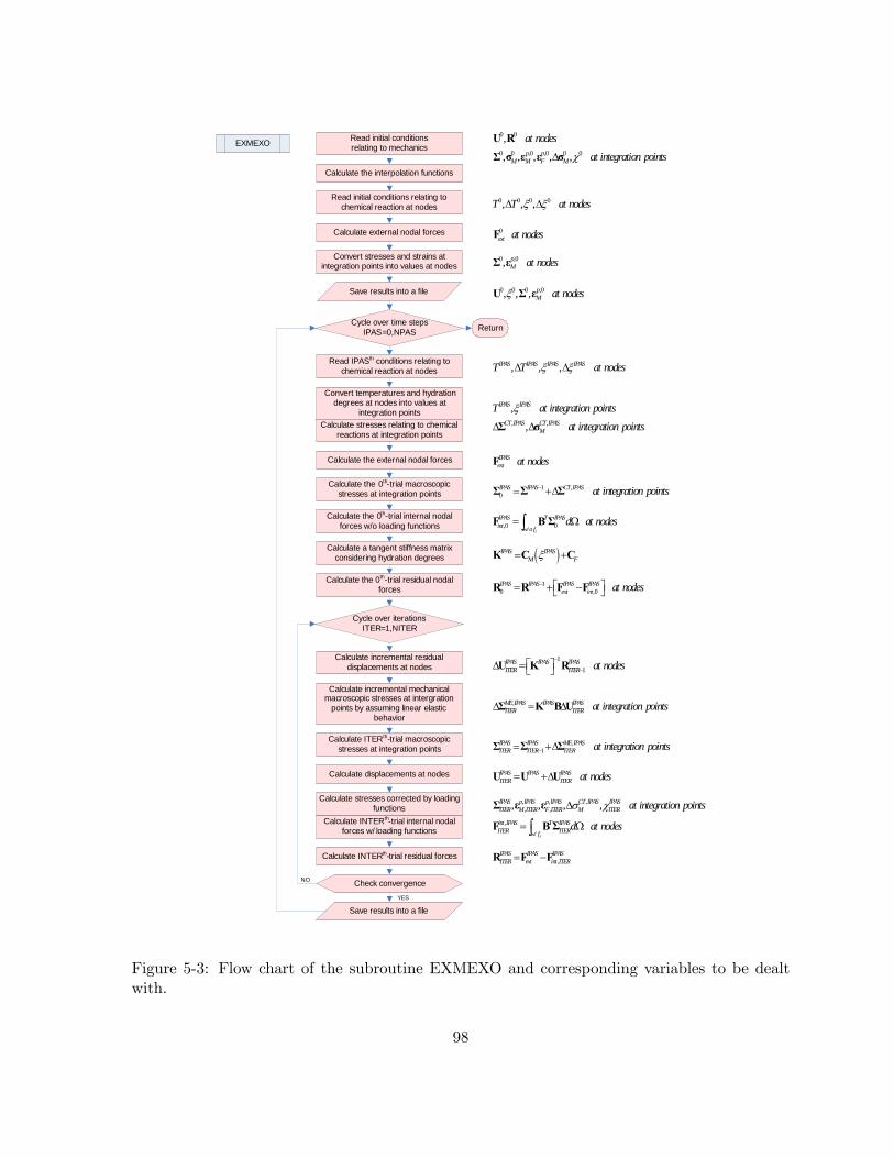
0 0
0 0 ,0 ,0 0 0
,, , , , ,p p
M M F M
at nodesat integration pointsχ∆
U RΣ σ ε ε σ
0 0 0 0, , ,T T at nodesξ ξ∆ ∆
0ext at nodesF
0 ,0, pM at nodesΣ ε
0 0 0 ,0, , , pM at nodesξU Σ ε
, , ,IPAS IPAS IPAS IPAST T at nodesξ ξ∆ ∆
, ,
,,
IPAS IPAS
CT IPAS CT IPASM
T at integration pointsat integration points
ξ
∆ ∆Σ σ
IPASext at nodesF
1 ,0IPAS IPAS CT IPAS at integration points−= +∆Σ Σ Σ
,0 0/ i
IPAS T IPASint w o f
d at nodes= Ω∫F B Σ
( )IPAS IPASM Fξ= +K C C
10 ,0IPAS IPAS IPAS IPAS
ext int at nodes− ⎡ ⎤= + −⎣ ⎦R R F F
1
1IPAS IPAS IPASITER ITER at nodes
−
−⎡ ⎤∆ =⎣ ⎦U K R
,ME IPAS IPAS IPASITER ITER at integration points∆ = ∆Σ K B U
,1
IPAS IPAS ME IPASITER ITER ITER at integration points−= +∆Σ Σ Σ
IPAS IPAS IPASITER ITER at nodes= +∆U U U
, , ,, ,
,
/
, , , ,
i
IPAS p IPAS p IPAS CT IPAS IPASITER M ITER F ITER M ITER
int IPAS T IPASITER ITERw f
at integration points
d at nodes
σ χ∆
= Ω∫Σ ε ε
F B Σ
,IPAS IPAS IPASITER ext int ITER= −R F F
EXMEXO Read initial conditionsrelating to mechanics
Cycle over time stepsIPAS=0,NPAS
Calculate the interpolation functions
Read initial conditions relating to chemical reaction at nodes
Calculate external nodal forces
Convert stresses and strains at integration points into values at nodes
Save results into a file
Read IPASth conditions relating to chemical reaction at nodes
Convert temperatures and hydration degrees at nodes into values at
integration points
Calculate the external nodal forces
Calculate the 0th-trial macroscopic stresses at integration points
Calculate the 0th-trial internal nodal forces w/o loading functions
Calculate a tangent stiffness matrix considering hydration degrees
Calculate the 0th-trial residual nodal forces
Calculate incremental residual displacements at nodes
Calculate incremental mechanical macroscopic stresses at intergration
points by assuming linear elastic behavior
Calculate displacements at nodes
Calculate stresses corrected by loading functions
Calculate INTERth-trial residual forces
Check convergence
Save results into a file
Calculate stresses relating to chemical reactions at integration points
Cycle over iterationsITER=1,NITER
Calculate INTERth-trial internal nodal forces w/ loading functions
Return
Calculate ITERth-trial macroscopic stresses at integration points
NO
YES
Figure 5-3: Flow chart of the subroutine EXMEXO and corresponding variables to be dealtwith.
98
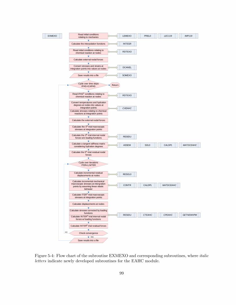
EXMEXO Read initial conditionsrelating to mechanics
Cycle over time stepsIPAS=0,NPAS
Calculate the interpolation functions
LEMEXO
INTEGR
RDTEXORead initial conditions relating to chemical reaction at nodes
Calculate external nodal forces
Convert stresses and strains at integration points into values at nodes
Save results into a file
DCANEL
SOMEXO
RDTEXORead IPASth conditions relating to chemical reaction at nodes
Convert temperatures and hydration degrees at nodes into values at
integration points CVEAHC
Calculate the external nodal forces
Calculate the 0th-trial macroscopic stresses at integration points
Calculate the 0th-trial internal nodal forces w/o loading functions RESIDU
Calculate a tangent stiffness matrix considering hydration degrees ASSEM SOL0
Calculate the 0th-trial residual nodal forces
Calculate incremental residual displacements at nodes RESOL0
Calculate incremental mechanical macroscopic stresses at intergration
points by assuming linear elastic behavior
CALDP1 MATDCEAHC
CONTR CALDP1 MATDCEAHC
Calculate displacements at nodes
Calculate stresses corrected by loading functions
RESIDU CTEAHC CPEAHC GETNEWVPM
Calculate INTERth-trial residual forces
Check convergence
Save results into a file
Calculate stresses relating to chemical reactions at integration points
Cycle over iterationsITER=1,NITER
Calculate INTERth-trial internal nodal forces w/ loading functions
Return
PREL0 LEC119 IMP119
Calculate ITERth-trial macroscopic stresses at integration points
NO
YES
Figure 5-4: Flow chart of the subroutine EXMEXO and corresponding subroutines, where italicletters indicate newly developed subroutines for the EAHC module.
99

(a)
(b)
Figure 5-5: Mesh design and boundary conditions of the uniaxial tension test simulation usingaxisymmetric elements: (a) Single element, (b) Fifty elements.
100

(a)
(b)
Hydration Degree = 0.25
0
1
2
3
0 1 2 3 4
Strain [1/1000]
Str
ess
[MP
a]
Analytical SolutionSimulation w/ a Single ElementSimulation w/ Fifty Elements
Hydration Degree = 0.25
0
1
2
0.0 0.1 0.2
Strain [1/1000]
Str
ess
[MP
a]
Analytical SolutionSimulation w/ a Single Element
Simulation w/ Fifty Elements
Figure 5-6: ξ = 0.25: uniaxial response of finite element simulations compared with the ana-lytical simulations: (a) Entire stress-strain curve, (b) Focus on first cracking behavior.
101

(a)
(b)
Hydration Degree = 0.5
0
2
4
6
0 2 4 6
Strain [1/1000]
Str
ess
[MP
a]
Analytical SolutionSimulation w/ a Single ElementSimulation w/ Fifty Elements
Hydration Degree = 0.5
0
2
4
0.0 0.1 0.2
Strain [1/1000]
Str
ess
[MP
a]
Analytical SolutionSimulation w/ a Single Element
Simulation w/ Fifty Elements
Figure 5-7: ξ = 0.5: uniaxial response of finite element simulations compared with the analyticalsimulations: (a) Entire stress-strain curve, (b) Focus on first cracking behavior.
102

(a)
(b)
Hydration Degree = 0.75
0
3
6
9
0 2 4 6 8
Strain [1/1000]
Str
ess
[MP
a]
Analytical SolutionSimulation w/ a Single ElementSimulation w/ Fifty Elements
Hydration Degree = 0.75
0
2
4
6
0.0 0.1 0.2 0.3
Strain [1/1000]
Str
ess
[MP
a]
Analytical SolutionSimulation w/ a Single Element
Simulation w/ Fifty Elements
Figure 5-8: ξ = 0.5: uniaxial response of finite element simulations compared with the analyticalsimulations: (a) Entire stress-strain curve, (b) Focus on first cracking behavior.
103

(a)
(b)
Hydration Degree = 1.0
0
4
8
12
0 2 4 6 8 10
Strain [1/1000]
Str
ess
[MP
a]
Analytical SolutionSimulation w/ a Single ElementSimulation w/ Fifty Elements
Hydration Degree = 1.0
0
2
4
6
8
0.0 0.1 0.2 0.3
Strain [1/1000]
Str
ess
[MP
a]
Analytical SolutionSimulation w/ a Single Element
Simulation w/ Fifty Elements
Figure 5-9: ξ = 1.0: uniaxial response of finite element simulations compared with the analyticalsimulations: (a) Entire stress-strain curve, (b) Focus on first cracking behavior.
104
5.3 Chapter Summary
This chapter describes the computational development of the early-age UHPC constitutive
model into the EAHC finite element module. The module is embedded into a commercial
finite element program, CESAR-LCPC. The EAHC module allows users to model early-age
UHPC structures. Finite element formulation including finite element equations and the re-
turn mapping algorithm is presented in detail with flowcharts of executable subroutines and
corresponding variables. Lastly, the proposed model is verified through simulations of uniax-
ial tension tests, showing an excellent agreement with the analytical solutions and very good
convergence between different mesh densities.
105

Part III
ENGINEERING APPLICATION
106

Chapter 6
EARLY-AGE 3-D UHPC MODEL
VALIDATION
During the recent manufacturing of a UHPC-girder, several cracks were observed in the deck
and web of the girder. Several hypothesis for the origin of this cracking were discussed, raising
questions whether the observed cracking was a consequence of the casting method, the prestress
application or formwork removal procedure. In this Chapter, we try to address these questions
by using the novel thermo-chemo-mechanical UHPC model. At the same time, the case study of
the UHPC bridge girder will serve for validation of our model to ultimately answer the question,
it is possible to predict and mitigate - by means of our advanced simulation tools - the risk
of early-age UHPC cracking. What we present here as well, is the whole procedure of using
our model, which includes the determination of the input parameters for both thermo-chemical
and thermo-chemo-mechanical problem, boundary conditions, application of prestressing, and
interpretation of simulation results.
6.1 Overview of Application
The bridge we study here is the prototype UHPC bridge which was developed at MIT for
the Federal High-Way Administration [18]. The bridge was optimized by means of model-
based simulation for relevant traffic loads and dead weight. This type of UHPC bridge has
the potential to be used throughout the U.S. for the next generation of US-Highway Bridge
107

Figure 6-1: MIT optimized DuctalTM bridge girder section (unit: inch) [20].
Girders. The section dimensions of the prestressed bridge girder are shown in Figure 6-1.
The bridge is 21 m (70 ft) long, and 22 strands are employed for prestress through its bottom
flange producing 2.4 MN (537 kips) of effective prestress. Figure 6-2 shows the configuration
of the formwork, which is composed of three parts: an inner formwork, an outer formwork, and
the bottom. This complex type of formwork was introduced in order to reduce autogenous
shrinkage during the casting procedure, because the considered UHPC material is known to
show considerable autogenous shrinkage. The bridge was cast by Prestress Service Inc. [PSi]
with the collaboration of Federal Highway Administration [FHWA] and Lafarge North America.
The construction was carried out over the period of October 11, 2003 to January 31, 2004.
When the bridge was moved out of its formwork, several cracks were observed in the deck
and web of the girder. Especially, relatively large cracks normal to the longitudinal direction
were observed (see Figure 6-3). The purpose of this engineering application is to validate the
108
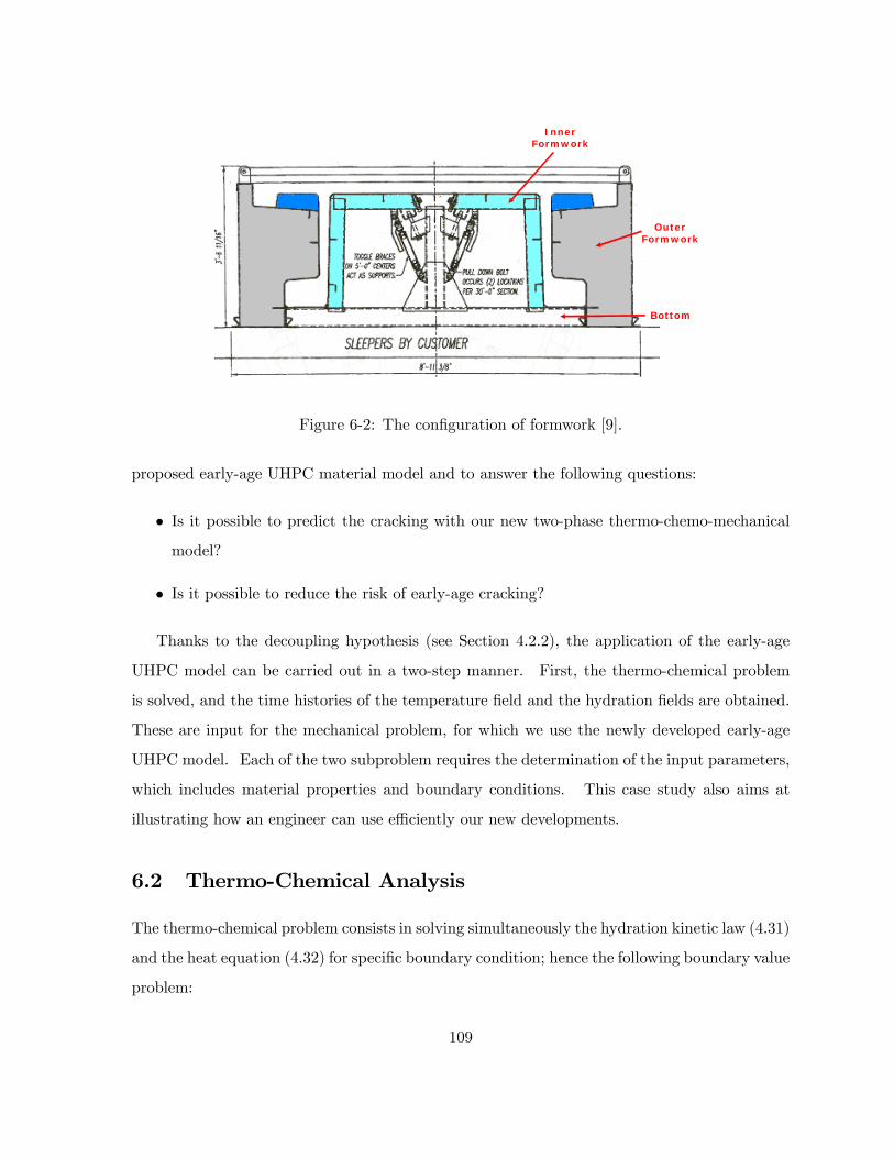
Inner Formwork
Outer Formwork
Bottom
Figure 6-2: The configuration of formwork [9].
proposed early-age UHPC material model and to answer the following questions:
• Is it possible to predict the cracking with our new two-phase thermo-chemo-mechanical
model?
• Is it possible to reduce the risk of early-age cracking?
Thanks to the decoupling hypothesis (see Section 4.2.2), the application of the early-age
UHPC model can be carried out in a two-step manner. First, the thermo-chemical problem
is solved, and the time histories of the temperature field and the hydration fields are obtained.
These are input for the mechanical problem, for which we use the newly developed early-age
UHPC model. Each of the two subproblem requires the determination of the input parameters,
which includes material properties and boundary conditions. This case study also aims at
illustrating how an engineer can use efficiently our new developments.
6.2 Thermo-Chemical Analysis
The thermo-chemical problem consists in solving simultaneously the hydration kinetic law (4.31)
and the heat equation (4.32) for specific boundary condition; hence the following boundary value
problem:
109

Figure 6-3: Cracking observed during casting, which runs from the deck to the neutral axis [9].
dξ
dt= A (ξ) exp
∙− Ea
RT
¸in Ω (6.1)
C∂T
∂t= K∇2T + L
dξ
dtin Ω (6.2)
q · n = λ (T − Text) on ∂Ω
where q · n is the heat out-flux through the surfaces of the structure. These equations are
implemented in CESAR-LCPC as module TEXO. Equations (6.1) and (6.2) require the de-
termination of the following input parameters: volume heat capacity C, heat conductivity K,
latent heat of hydration L = C¡T ad∞ − T ad
0
¢(where T ad
∞ −T ad0 is the adiabatic temperature rise;
see Section 3.3.1), the hydration activation constant Ea/R; the normalized affinity function
A (ξ) (see Section 3.3); and finally the heat exchange coefficient λ of the formwork employed.
These model input parameters are obtained first, before discussing the simulation results:
the time history of the temperature field T (x, t), and the hydration degree field ξ (x, t) in the
110

Cover
Inner-formOuter-form
Bottom
Cover
Inner-formOuter-form
Bottom
Figure 6-4: Mesh composed of 894 2-D plain strain elements and 300 exchange elements denotedas black straight lines.
structure. The simulation results are then compared with temperature measurements carried
out during casting on-site, providing a means to validate our input parameters.
6.2.1 Thermal Boundary Conditions
Figure 6-4 shows the mesh employed in the 2-D simulation of the bridge girder section. For
symmetry reason, only half of the section is modeled, prescribing a zero heat-flux along the
symmetry axis. The other surfaces are modeled by linear exchange elements defined by (6.2)
(displayed in Figure 6-4 as black straight lines) which we use to simulate the loss of heat through
the formworks. These exchange conditions allow us to simulate in detail the casting procedure.
At the site, the formworks were successively removed, and each formwork removal corre-
sponds to a change of the thermal boundary conditions. At the beginning, both the inner
formwork and the outer formwork were attached to the structure. The inner formwork was
first removed 40 hours after casting, and the outer formwork was removed 50 hours after cast-
ing. This process is illustrated in Figure 6-5, displaying four phases which are considered in
our simulations. Even though there is no difference in thermal boundary conditions before and
111

Phase 10~40h
Phase 240~50h
Phase 2Phase 240~50h
Phase 3Before Prestress
50~65h
Phase 3Phase 3Before Prestress
50~65h
Phase 4After Prestress
65h~
Phase 4Phase 4After Prestress
65h~
Figure 6-5: Progressive formwork removal inducing change in thermal boundary conditions.
after the application of the prestressing force, we separately considered these two phase because
the prestressing corresponds to a change in mechanical boundary conditions. For each phase,
different exchange coefficients were used for each part of the formwork, and they are summarized
in Table 6.1. Using standard values of the literature [16], the exchange coefficient1 was set to
λ = 14 kJ/¡hr ×m2 ×K
¢for the surface exposed to the air, and λ = 10 kJ/
¡hr ×m2 ×K
¢for surfaces with steel formwork. These exchange coefficient define the heat out-flux over the
surface according to (6.2). The second input parameter required is the external temperature.
This external temperature was measured during the casting process, and Figure 6-6 shows the
simplified external temperature history we employed in simulations. Finally, after applying the
prestressing force, the bridge girder was transported to an open field, and the formwork were
removed for another bridge girder casting.
1 It was reported that the bridge girder was placed in a tent during the casting process in order to preventharsh external weather conditions [9]. Thus, this situation was considered as a non-ventillated condition for theexchange coefficient.
112

Exchange Coefficientλ [KJ/
¡hr ×m2 ×K
¢]
Cover Inner-form Outer-form BottomPhase 1 14 10 10 10Phase 2 14 14 10 10Phase 3 14 14 14 14Phase 4 14 14 14 14
Table 6.1: Values of exchange coefficients for each phase.
History of External Temperature
0
10
20
30
40
0 20 40 60 80
Time [hours]
Tem
pera
ture
[°
C]
PHASE 1PHASE 2PHASE 3PHASE 4
inner-formremoved
outer-formremoved
prestressapplied
Figure 6-6: History of external temperature [9].
113

6.2.2 Thermal Properties and Adiabatic Temperature Curve
The second set of input parameters for the thermo-chemical problem includes the thermal
properties and the normalized affinity of the UHPC material, here DuctalTM .
Volume Heat Capacity
Since the volume heat capacity of steel (C = 3, 500 kJ/¡m3 ×K
¢) is somewhat greater than
the volume heat capacity of normal concrete (C = 2, 400 kJ/¡m3 ×K
¢), it is reasonable to set
the volume heat capacity of a steel fiber reinforced UHPC to a slightly greater value than that
of ordinary concrete:
C = 2, 700 kJ/¡m3 ×K
¢(6.3)
Heat Conductivity
The heat conductivity of UHPC is estimated to be on the same order of that of ordinary concrete
[16]:
KunreUHPC = 5 kJ/ (hr ×m×K) (6.4)
This values is employed for the unreinforced deck and web of the girder. In return, the bottom
flange is highly filled with prestressing cables that increase the heat conductivity, which is set
to:
KreinUHPC = 8 kJ/ (hr ×m×K) (6.5)
Adiabatic Temperature Curve
We have seen in Section 3.3 that the normalized affinity A (ξ) can be equally accessed by either
an adiabatic temperature curve or an isothermal strength evolution law. In the simulations,
the adiabatic temperature curve T ad (t) is used as input to determine A (ξ). However, the
adiabatic temperature for DuctalTM was not available, but fortunately the quasi-isothermal
strength evolution was measured on-site, which we used to determine the normalized affinity
from (see Section 3.3.2):
A (ξ) = exp
∙Ea
RT iso
¸1
f iso∞ − f0
df iso
dt(6.6)
114

Here, f iso (t) is the compressive strength growth curve, which we determine by interpolating
the compressive strength values measured on-site2. This fitting is displayed in Figure 6-7 (a),
since the hydration degree can be determined from (see Section 3.3.2):
ξ (t) =f iso (t)− f0f iso∞ − f0
(6.7)
We can determine the normalized affinity curve, as displayed in Figure 6-7 (b). Finally, using
the determined affinity curve in the heat equation (6.2) for adiabatic conditions, we obtain after
integration the adiabatic temperature curve T ad (t)− T ad0 :
T ad (t)− T ad0 =
³T ad∞ − T ad
0
´Z t
0A (ξ) exp
∙− Ea
RT ad (s)
¸ds (6.8)
where:
ξ (t) =T ad (t)− T0T ad∞ − T0
(6.9)
The procedure requires some iteration, and the result is displayed in Figure 6-7 (c).
This iterative procedure requires as input the activation energy or more precisely a reference
value for the dimensionless number Ea/¡RT iso
¢in the strength rate - normalized affinity rela-
tion (6.6). Inspired from typical values for the activation energy for ordinary concrete Ea/R
= 4, 000− 4, 150 K, we choose:
Ea
RT iso=4000
273=4150
283= 14.7 (6.10)
It should be noted that fixing the values of Ea/¡RT iso
¢ensures that the normalized affinity
curve obtained from the isothermal strength growth is the same irrespective of the temperature
T iso. This is constant with the fact that the normalized affinity curve is an intrinsic material
property which is independent of thermal boundary conditions. On the other hand, the choice
of the activation energy (Ea/R = 4, 000K or Ea/R = 4, 150K) has some effects on the rate of
the adiabatic temperature rise. This is illustrated in Figure 6-8. While the normalized affinity
curve A (ξ) in the same (by construction, see Figure 6-8 (a)), a higher activation energy leads to
2 It was reported that the compressive strength specimen were placed in the tent where the bridge girder wascast [9].
115

(a)
(b)
(c)
Simulated Evolution of Adiabatic Temperature
0
40
80
120
0 20 40 60 80 100
Tim [hours]
Tem
pera
ture
[°C
]
Simulated Evolution ofAdiabatic Temperature
External Temperature
Comparison of Affinities
0
5
10
15
0 0.2 0.4 0.6 0.8 1
Hydration Degree [1]
Aff
inity
[1/s
ec]
From Simulated AdiabaticTemperature
From InterpolatedIsothermal Strength
Evolution of Compressive Strength
0
50
100
150
200
0 500 1000 1500 2000 2500
Age [hours]Com
pres
sive
Str
engt
h [M
Pa]
Interpolated Evolution ofCompressive Strength
Experimental Values
Figure 6-7: Procedure to obtain the simulated adiabatic temperature curve from the isothermalcompressive strenght growth: (a) Evolution of the compressive strength, (b) Comparison of theaffinities from simulated adiabatic temperature and interpolated quasi-isothermal compressivestrength, (c) Determined evolution of the adiabatic temperature (Ea/R = 4, 000 K).
116

slower evolution of the adiabatic temperature rise (Figure 6-8 (b)), because a higher activation
energy decreases the reaction rate (6.1). While the difference in between the two temperature
curve is not enormous, it is not insignificant, thus high-lighting the necessity of an adiabatic
temperature test for the UHPC material. Such an adiabatic temperature curve in combination
with the isothermal strength growth determined on-site would provide more accurate values of
the activation energy.
In the absence of this adiabatic temperature curve for DuctalTM , we will consider both
adiabatic temperature curves in the simulation. A first-order engineering validation of the
here determined normalized affinity curve is obtained by comparing the simulated temperature
history with temperature values measure on-site.
6.2.3 Simulation Results and Validation
Temperatures were measured at three points in the structure: the deck, the web and the bottom
flange, as shown in Figure 6-9. Figure 6-10 shows the temperature history measured on site.
The bottom flange showed a higher temperature than other measurement points because it has
the characteristics of a massive concrete structure. The maximum temperature in the bottom
flange is 52 C. The maximum temperature for each location occurred in the time interval
between 58 and 63 hours after casting. The temperature was measured on site until the
prestressing force was applied.
The simulated temperature histories are displayed in Figure 6-11, obtained with an acti-
vation energy of Ea/R = 4, 000K. As expected, the highest temperature rise occurs in the
bottom flange with a maximum temperature of 51 C, which compares very well with the mea-
sured value of 52 C. This maximum temperature occurs in the time interval between 53 and
58 hours, which is close to the measured time of 58 − 63 hours after casting. The slightly
premature occurrence of the maximum temperature can be attributed to the choice of the ac-
tivation energy of Ea/R = 4, 000K. In fact, Figure 6-12 display a comparison of the measured
temperatures and simulated results obtained respectively with Ea/R = 4, 000 K (Figure 6-12
(a)) and Ea/R = 4, 150 K (Figure 6-12 (b)). The simulations carried out with a higher acti-
vation energy predict more accurately the time occurrence of the maximum temperature. On
the other hand, the maximum temperature in the bottom flange is slightly underestimated in
117

Simulated Evolution of Adiabatic Temperature
0
20
40
60
80
100
20 40 60 80 100
Tim [hours]
Tem
per
ature
[°C
]
Simulated Evolutionof AdiabaticTemperature withEa/R=4000K
Simulated Evolutionof AdiabaticTemperature withEa/R=4150K
ExternalTemperature
Comparison of Affinities
0
5
10
15
0 0.2 0.4 0.6 0.8 1Hydration Degree [1]
Affin
ity
[1/s
ec]
From InterpolatedIsothermalStrength
From SimulatedAdabaticTemperature withEa/R=4000K
From SimulatedAdabaticTemperature withEa/R=4150K
(a)
(b)
Figure 6-8: (a) Comparison of two affinities from simulated adiabatic temperature (Ea/R =4, 000K and 4, 150K) and the extrapolated quasi-isothermal compressive strength, (b) Com-parison of two simulated adiabatic temperature curves (Ea/R = 4, 000K and 4, 150K).
118
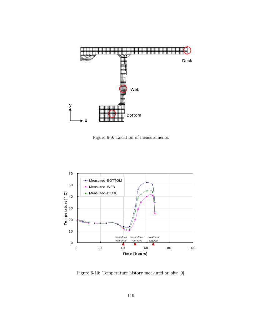
Bottom
Web
Deck
x
y
x
y
Figure 6-9: Location of measurements.
0
10
20
30
40
50
60
0 20 40 60 80 100
Time [hours]
Te
mpe
ratu
re[°
C]
Measured-BOTTOM
Measured-WEB
Measured-DECK
inner-formremoved
outer-formremoved
prestressapplied
Figure 6-10: Temperature history measured on site [9].
119

0
10
20
30
40
50
60
0 20 40 60 80 100
Time [hours]
Te
mpera
ture
[° C
]
BOTTOMWEBDECKExternal Temperature
inner-formremoved
outer-formremoved
prestressapplied
Figure 6-11: Temperature history from the simulation with Ea/R = 4, 000 K.
the simulation result obtained with Ea/R = 4, 150 K (max [T − T0] = 49C vs. the measured
52 C). Note that the temperature histories for both web and deck are little affected by the
value of the activation energy, and are very similar, because their dimensions are similar.
For the mechanical simulations of stresses and deformations, we choose the Ea/R = 4, 000K
simulation results. This choice is based on an overall comparison of the simulated temperature
values vs. measured values, displayed in Figures 6-12 and 6-13. While Figure 6-13 shows that
both simulation results give comparable correct predictions regarding temperature distribution,
the Ea/R = 4, 000 K simulation results (Figure 6-12) give a closer agreement with the max-
imum temperature measured on-site. On the other hand, the Ea/R = 4, 000 K simulations
overestimate the temperature in the web.
Finally, Figure 6-14 shows a typical example of a simulated temperature distribution for
Ea/R = 4, 000K at the time of prestress application. This instant will turn out to be important.
The maximum temperature difference between the bottom flange and web is around 10 K. As
expected, the bottom flange has a higher temperature, compared to the deck and the web.
Moreover, a local temperature gradient effect can be seen: the temperature at the surface is
120

0
10
20
30
40
50
60
0 20 40 60 80 100
Time [hours]
Tem
pera
ture
[° C
]
Simulated-BOTTOMSimulated-WEBSimulated-DECKMeasured-BOTTOMMeasured-WEBMeasured-DECK
inner-formremoved
outer-formremoved
prestressapplied
0
10
20
30
40
50
60
0 20 40 60 80 100
Time [hours]
Tem
pera
ture
[° C
]
Simulated-BOTTOMSimulated-WEBSimulated-DECKMeasured-BOTTOMMeasured-WEBMeasured-DECK
inner-formremoved
outer-formremoved
prestressapplied
0
10
20
30
40
50
60
0 20 40 60 80 100
Time [hours]
Tem
pera
ture
[° C
]
Simulated-BOTTOMSimulated-WEBSimulated-DECKMeasured-BOTTOMMeasured-WEBMeasured-DECK
inner-formremoved
outer-formremoved
prestressapplied
0
10
20
30
40
50
60
0 20 40 60 80 100
Time [hours]
Tem
pera
ture
[° C
]
Simulated-BOTTOMSimulated-WEBSimulated-DECKMeasured-BOTTOMMeasured-WEBMeasured-DECK
inner-formremoved
outer-formremoved
prestressapplied
(a)
(b)
Figure 6-12: Comparison of on-site measured and simulated temperature histories: (a) Ea/R =4, 000 K, (b) Ea/R = 4, 150 K.
121

MeasuredTemperature Compared withSimulated Temperature
0
20
40
60
0 20 40 60
Measured Temperature [°C]
Sim
ula
ted T
em
pera
ture
[°
C]
Ea/R=4000KBottom
Ea/R=4000KWeb
Ea/R=4000KDeck
Ea/R=4150KBottom
Ea/R=4150KWeb
Ea/R=4150KDeck
Figure 6-13: Measured temperatures compared with simulated temperature.
122

x
y
x
y
. 10Max T K∆ ≈
Figure 6-14: Temperature distribution at the moment of prestress application.
lower than the inside temperature.
6.3 Two-Phase Thermo-Chemo-Mechanical Analysis
The time history of temperature distribution T (x, t) and hydration degree distribution ξ (x, t),
determined from the thermo-chemical analysis (see Section 6.2) serves as input for the me-
chanical analysis of stresses, deformation and permanent strains associated with cracking, that
develop during casting and hardening of the UHPC girder. This mechanical analysis is achieved
with the newly developed early-age UHPC module, detailed in Chapter 5 and implemented in
CESAR-LCPC.
6.3.1 Plane-Section Simulation
The mechanical simulations of the girder sections are carried out in 2-D, using the plane-section
assumption. It is assumed that the section remains plane during deformation, which is highly
relevant for beam-type structures. This assumption allows one to reduce the complete 3-D
simulation of the beam structure to 2-D simulations of the section, while considering the normal
123

forces and bending moments induced by the dead weight and the application of prestressing in
the statically determined structure.
The plane-section assumption ensures that the total strain in the z-direction (out-of-plane
direction) complies with the Bernoulli condition:
Ezz (x, y) =0z + yθx − xθy (6.11)
where 0z, θx and θy are the average strain in the z-direction and the curvatures around the
x- and y-axes, respectively. These three section unknowns need to be determined. To this
end, the global equilibrium in the section "A" is calculated, using the common definition of the
normal force and the bending moment:
N =
ZAΣ · ezdA (6.12)
M =
ZA(xex + yey)× (Σ · ez) dA (6.13)
where "×" denotes the cross product. The stress tensor in any part of the section can be
written as:
Σ = ΣPS + κ diagh1 1 1−ν
ν
iEzz (6.14)
where ΣPS is the total stress tensor corresponding to plane strain conditions (Ezz ≡ 0), and
κ (ξ) = νK0 (ξ)
(1− 2ν) (1 + ν)(6.15)
with K0 (ξ) = CM (ξ) + CF is the composite Young’s modulus. Use of (6.14) in (6.12) and
(6.13) leads to expressing the section equilibrium in the following form:
0 =
⎧⎪⎪⎪⎨⎪⎪⎪⎩NPS −Nd
MPSx −Md
x
MPSy −Md
y
⎫⎪⎪⎪⎬⎪⎪⎪⎭+1− ν
ν
⎡⎢⎢⎢⎣RA κ (ξ) dA
RA κ (ξ) ydA −
RA κ (ξ)xdAR
A κ (ξ) ydARA κ (ξ) y
2dA −RA κ (ξ)xydA
−RA κ (ξ)xdA −
RA κ (ξ)xydA
RA κ (ξ)x
2dA
⎤⎥⎥⎥⎦⎧⎪⎪⎪⎨⎪⎪⎪⎩
0z
θx
θy
⎫⎪⎪⎪⎬⎪⎪⎪⎭(6.16)
where (Nd, Mdx and Md
y ) are prescribed normal force and moments on the beam (dead weigth
and prestressing), while (NPS ,MPSx andMPS
y ) are obtained by application of (6.12) and (6.13)
124

to the plane-strain stress Σ→ ΣPS . In the mechanical calculation, relation (6.16) is solved
at every iteration, and the total stress in the section is corrected according to relation (6.14).
Finally, relation (6.12) is used to evaluate the longitudinal strain Ezz (t) at different points in
the section, for which measurements from the site are available.
6.3.2 Mechanical Boundary Conditions
Like every mechanical problem, the stress and deformation analysis of the UHPC girder at early
ages requires force and displacement boundary conditions as input.
Displacement Boundary Conditions
In the particular case of the early-age behavior of UHPC structures, the displacement boundary
conditions are defined by the formwork. More precisely, each formwork removal on-site corre-
sponds to a change in the displacement boundary conditions. For the four phases considered in
the thermo-chemical analysis (see Section 6.2.1, Figure 6-5), the displacements are set to zero
at those boundaries where a formwork is placed. The progressive formwork removal and the
corresponding change in displacement boundary conditions we consider in the simulations are
displayed in Figure 6-15. In this figure, straight lines represent a zero-displacement bound-
ary3 and the removal of the formwork from one phase to the other represents a release of this
zero-displacement boundary, so that the surface becomes stress-free (Σ · n = 0). The finite
element simulations are performed on the same mesh as the thermo-chemical analysis. The
zero-displacement in the symmetry axis of the section is due to symmetry considerations.
Force Boundary Condition
Beside the stress-free boundary condition at the free surfaces that relate to the formwork removal
procedure (see Figure 6-5), there are two further prescribed forces to be considered: the dead
weight and the prestress application. Since the girder remains on the formwork until it is lifted
out, the dead weight is of minor importance. In return, application of the prestressing (in Phase
4) leads to introduce both a normal force and bending moments. These effects are considered
3The zero-displacement means that displacements normal to the boundary are zero.
125

x
y
x
y
Phase 2
40~50h
Phase 2
40~50h
Phase 1
0~40h
Phase 1Phase 1
0~40h
Phase 3Before Prestress 50~65h
Phase 3Phase 3Before Prestress 50~65h
Phase 4After Prestress 65h~
Phase 4Phase 4After Prestress 65h~
Figure 6-15: Progressive formwork removal inducing a change in displacement boundary con-ditions.
126

in the simulations through relation (6.16), by letting:
Nd = −P
Mdx = Pey
Mdy = Pex
(6.17)
where P = 1.2 MN is the effective prestressing force for a half girder and (ex, ey) = (0.46 m,
0.13 m) is the distance between the center of gravity of the half section and the center of the
prestressing force. Conditions (6.17) are prescribed in the simulations in Phase 4.
6.3.3 Mechanical Material Properties
The second set of input parameters for the mechanical analysis is the set of properties required
by the two-phase early-age UHPC model. By construction, these are (see Section 4.2.4):
• The hardened UHPC properties: Elastic properties (CM , CF , M and ν) and strength
properties (σMt, σcrMt, σMc, σMb, σFt and σFc). These can be obtained from the test
data provided by the manufacturer.
• The thermo-chemical properties of UHPC: Thermal dilatation coefficients (αM and αF ),
chemical dilatation coefficient (βM and βF ) and the percolation threshold (ξ0) (see Section
4.1.1).
For the hardened UHPC properties, the model parameters of DuctalTM -Steel Fiber are
employed (see Table 2.4). In addition, Table 6.2 lists the thermo-chemical deformation prop-
erties we consider in the simulations. The thermal dilatation coefficient for both composite
phases are assumed to be the same. In return, only the composite matrix phase is assumed
to undergo chemical shrinkage. The value of βM = −8 × 10⁻⁴ is estimated from autogenous
shrinkage values for low water/cement ratio concrete in the open literature4 [3]. Finally, re-
4The value of βM = −8 × 10⁻⁴ yields maximum autogenous shrinkage of the composite matrix of =−800 µm/m. This value includes hydration shrinkage related to the Le Chatelier contraction and the shrinkageinduced by the hydric pressure that develop in the material at early-ages. Since we do not distinguish thesetwo phenomena, the maximum shrinkage induced is an upper bound to the actual autogenous shrinkage. Thisis appropriate with respect to the focus of our simulation: to evaluate the risk of early-age UHPC cracking.
127

Matrix Steel FiberThermal dilatationcoefficient [1/K]
αM = 1× 10⁻⁵ αF = 1× 10⁻⁵
Chemical shrinkagecoefficient [1]
βM = −8× 10⁻⁴ βF = 0
Percolationthreshold [1]
ξ0 = 0.1 -
Table 6.2: Thermo-chemical deformation properties of UHPC considered in the simulations.
garding the percolation threshold, we employ ξ = 0.1, as generally admitted in the early-age
concrete literature [25][26].
6.3.4 Validation
On-site, longitudinal strains (in the z-direction) were measured by strain gauges at the deck
and the bottom flange until the application of the prestressing. We use these measured values
for validation of the model and its implementation in the finite element program. Figure 6-
16 compares the recorded strain measurements with the longitudinal macroscopic strains Ezz
determined from the application of the plane-section model (6.11) in our simulations. The
simulated strain history at different points in the section shows a very good agreement with
the measured strains, except for the web. This is not surprising, given the discrepancy of
temperature we found in the thermo-chemical simulation. Figure 6-17 displays the simulated
results vs. the measured results of the deck and the bottom flange. The good agreement
here provides strong evidence that our new model gives a relatively accurate prediction of the
deformation behavior of the UHPC girder at early ages. Based on this validation, we can now
turn to the question, what caused the early-age cracking observed in the girder.
6.4 What Caused the Early-Age UHPC Cracking?
The crack were observed normal to the longitudinal direction (beam axis). Such cracks result
from a longitudinal stress excess. Thus, to answer the raised question, our main focus will be
on stresses and plastic strains in the longitudinal axis.
128

Time History of Strains (Ezz)
-1.0E-03
-8.0E-04
-6.0E-04
-4.0E-04
-2.0E-04
0.0E+00
2.0E-04
0 20 40 60 80 100
Time [hours]
Tota
l S
train
[1
]
Simulated-BOTTOMSimulated-WEBSimulated-DECKMeasured-BOTTOMMeasured-WEBMeasured-DECK
inner-formremoved
outer-formremoved
prestressapplied
Time History of Strains (Ezz)
-1.0E-03
-8.0E-04
-6.0E-04
-4.0E-04
-2.0E-04
0.0E+00
2.0E-04
0 20 40 60 80 100
Time [hours]
Tota
l S
train
[1
]
Simulated-BOTTOMSimulated-WEBSimulated-DECKMeasured-BOTTOMMeasured-WEBMeasured-DECK
inner-formremoved
outer-formremoved
prestressapplied
Figure 6-16: Simulated longitudinal strain histories compared with the strain measurements onsite.
129

Measured Strains Compared withSimulated Strains
-4.0E-04
-3.0E-04
-2.0E-04
-1.0E-04
0.0E+00
1.0E-04
-4.0E-04 -3.0E-04 -2.0E-04 -1.0E-04 0.0E+00 1.0E-04
Measured Strains [1]
Sim
ula
ted
Str
ain
s [1
]
BOTTOM
DECK
Measured Strains Compared withSimulated Strains
-4.0E-04
-3.0E-04
-2.0E-04
-1.0E-04
0.0E+00
1.0E-04
-4.0E-04 -3.0E-04 -2.0E-04 -1.0E-04 0.0E+00 1.0E-04
Measured Strains [1]
Sim
ula
ted
Str
ain
s [1
]
BOTTOM
DECK
Figure 6-17: Measured strains compared with simulated strains.
130

6.4.1 Stress and Plastic Strain Distributions
The longitudinal macroscopic stress (Σzz) from the simulation is first investigated. In Phase 1
and 2, the mechanical properties are not developed enough to show considerable stress values, as
captured in Figure 6-18. However, the stress starts to show considerable magnitudes beginning
in Phase 3. Figure 6-19 (a) shows a contour map of the stress at the end of phase 3, right
before the application of prestressing. Due to local temperature gradient effects, some parts
are in compression, particularly the bottom flange where the temperature is the highest (see
Figure 6-14). Since there is no external loading during the casting process5, the structure is
in a self-equilibrium state. As a consequence, the compression in the deck and bottom flange
is balanced by tension in the web. Moreover, tension also exists near the surfaces due to
temperature effects. Figure 6-19 (b) corresponds to the stress state right after the prestressing
force application (Phase 4). Now, the bottom flange and the web are in compression, but the
deck is mostly in tension. Due to some eccentricity of the prestressing force, the inner part of
the deck shows larger tensile stress values than the outer part.
Since the plastic strain in the composite matrix corresponds to the cracking in the UHPC
structure, the investigation of the matrix plastic strain provides a means to evaluate the risk of
cracking during the casting process. There is no plastic strain in Phase 1 and Phase 2 (Figure
6-20), because the mechanical properties are not developed enough to show considerable stress
values. Hence, there is no cracking in the structure. However, after removing the inner and
outer formwork, some plastic strains occur as illustrated in Figure 6-21. Before application
of the prestressing force, there exist some plastic strains localized on the deck surface and on
the web surface. These localized plastic strains can be attributed to the local temperature
gradients close to the surface, which may induce some small surface cracks. After prestress
application, the plastic strains in the deck increase as a consequence of the tension (Figure 6-19
(b)) in the deck induced by prestressing. On the other hand, the plastic strains in the web do
not change, since the web is in compression after prestress application as illustrated in Figure
6-19 (b).
5Dead weight is neglected.
131

at 35 h
Phase 1at 35 h
Phase 1at 35 h
Phase 1
at 45 h
Phase 2at 45 h
Phase 2at 45 h
Phase 2
(a)
(b)
Figure 6-18: Distribution of the longitudinal macroscopic stress (Σzz): (a) At 35 hours aftercasting in Phase 1, (b) At 45 hours after casting in Phase 2.
132

at 65 h
Phase 3Before Prestress at 65 h
Phase 3at 65 h
Phase 3Before Prestress
at 65.25 h
Phase 4After Prestress at 65.25 h
Phase 4at 65.25 h
Phase 4After Prestress
(a)
(b)
Figure 6-19: Distribution of the longitudinal macroscopic stress (Σzz): (a) Before prestressapplication (Phase 3), (b) After prestress application (Phase 4).
133

at 35 h & 45 h
Phase 1 & 2at 35 h & 45 h
Phase 1 & 2
Figure 6-20: Distribution of the longitudinal plastic strain in the composite matrix (εpM,zz) atboth 35 and 45 hours after casting in Phase 1 and 2, respectively.
6.4.2 Stress and Plastic Strain Before and After Applying Prestress
In order to fully understand what happened, we take a closer look on the stress and plastic
strain profiles along the cross section of the web and the deck. Figure 6-22 (a) displays the
longitudinal macroscopic stress Σzz profile along the web. Before prestress application, most
of the web is in tension while the center of both deck and bottom flange are in compression.
As stated before, this phenomenon is a typical example of a self-balanced stress state. The
higher temperatures in the bottom flange and in the deck lead to compression that is balanced
by tension in the web. After the application of the compressive prestressing force introduced
through the bottom flange, the deck is now in tension while the web and the bottom flange are
in compression.
Figure 6-22 (b) shows the cracking strains that are produced by these stresses. The shown
plastic strains (εpM,zz) imply cracks that open in the z-direction. Before applying the pre-
stressing force, small plastic strains already exist in the web and the bottom flange. After the
prestressing force application, there is no additional plastic strain created because the web and
the bottom flange are in compression. This confirms that the plastic strains along the web are
134

Before Applying Prestress
After Applying Prestress
SA
ME
INC
REA
SE
Figure 6-21: Distribution of the longitudinal plastic strain in the composite matrix (εpM,zz) inthe web (left) and the deck (right) before and after presstress application.
135

the consequence of the stresses generated due to differential thermal deformation and chemical
shrinkage, but the magnitude of the strains is very small, i.e. maxhεpM,zz
i∼ 10−5.
Figure 6-23 displays longitudinal stresses and plastic strains along the deck surface. As
expected from Figure 6-19 (a), most of the deck surface, prior to prestress application, is in
tension due to local temperature gradients over the deck thickness (Figure 6-23 (a)). There is a
small stress drop in the middle of the deck, which can be attributed to some plastic deformation
as a result of these surface temperature gradients. After prestress application, the deck is
mostly in tension. An important stress drop is now detected in the center of the deck. The
source of this stress drop becomes clear, if we compare this result with that of chemo-elastic
simulations which are also displayed in Figure 6-23 (a). The comparison shows a considerable
stress drop (max [∆Σzz] ∼ 2 MPa) in the center of the deck. Hence, this stress drop can
be identified as a clear consequence of cracking, and we can expect some plastic strains in the
deck.
Figure 6-23 (b) shows the longitudinal plastic strain (εpM,zz) profile in the deck. Small
plastic strains already exist in the center of the deck before applying the prestressing force.
However, the magnitude of these strains is roughly on the same order as the plastic strains
observed along the web, i.e. maxhεpM,zz
i∼ 10−5. These strains are, again, due to local
thermal gradient effects. In return, the application of the prestressing force increases the
plastic strains by a factor of five! This increase allows us to conclude that the risk of cracking
was increased considerably by prestress application, which appears to us as the main source of
cracking.
6.4.3 Time History of Simulation Results
To make the picture complete, Figure 6-24 displays the time history of the stress and the
plastic strains for the three locations shown in Figure 6-9 (deck, web and bottom flange). As
we expected, the Σzz-time history displayed in Figure 6-24 (a) shows a big jump in stresses due
to the prestressing force application, which leads to compression in the web and the bottom
flange, and to tension in the deck. However, as time goes on, a stress re-distribution occurs
due to the stiffness change of the UHPC, which release some compression in the bottom flange
that is added to the web.
136

Szz along Web
0.0
0.2
0.4
0.6
0.8
-20 -15 -10 -5 0 5
Stress [MPa]
Heig
ht
of
Gir
der
[m] Before Prestressing
After Prestressing
epsilon_(M,zz) along Web
0.0
0.2
0.4
0.6
0.8
-3.0E-06 1.0E-06 5.0E-06 9.0E-06 1.3E-05
Plastic Strain [1]
Heig
ht
of
Gir
der
[m]
Before Prestressing
After Prestressing
(a)
(b)
Szz along Web
0.0
0.2
0.4
0.6
0.8
-20 -15 -10 -5 0 5
Stress [MPa]
Before Prestressing
After Prestressing
epsilon_(M,zz) along Web
0.0
0.2
0.4
0.6
0.8
-3.0E-06 1.0E-06 5.0E-06 9.0E-06 1.3E-05
Plastic Strain [1]
Before Prestressing
After Prestressing
(a)
(b)
Szz along Web
0.0
0.2
0.4
0.6
0.8
-20 -15 -10 -5 0 5
Stress [MPa]
Heig
ht
of
Gir
der
[m] Before Prestressing
After Prestressing
Szz along Web
0.0
0.2
0.4
0.6
0.8
-20 -15 -10 -5 0 5
Stress [MPa]
Heig
ht
of
Gir
der
[m] Before Prestressing
After Prestressing
epsilon_(M,zz) along Web
0.0
0.2
0.4
0.6
0.8
-3.0E-06 1.0E-06 5.0E-06 9.0E-06 1.3E-05
Plastic Strain [1]
Heig
ht
of
Gir
der
[m]
Before Prestressing
After Prestressing
epsilon_(M,zz) along Web
0.0
0.2
0.4
0.6
0.8
-3.0E-06 1.0E-06 5.0E-06 9.0E-06 1.3E-05
Plastic Strain [1]
Heig
ht
of
Gir
der
[m]
Before Prestressing
After Prestressing
(a)
(b)
Szz along Web
0.0
0.2
0.4
0.6
0.8
-20 -15 -10 -5 0 5
Stress [MPa]
Before Prestressing
After Prestressing
epsilon_(M,zz) along Web
0.0
0.2
0.4
0.6
0.8
-3.0E-06 1.0E-06 5.0E-06 9.0E-06 1.3E-05
Plastic Strain [1]
Before Prestressing
After Prestressing
(a)
(b)
Figure 6-22: (a) Longitudinal macroscopic stress profile along the web, (b) Longitudinal plasticstrain in the composite matrix along the web.
137

Szz on Deck
-2.0
0.0
2.0
4.0
6.0
0.0 0.3 0.6 0.9 1.2
Width of Deck [m]
Str
ess
[M
Pa]
Before Prestressing
After Prestressing
After Prestressing-Elastic
epsilon_(M,zz) on Deck
-2.0E-05
0.0E+00
2.0E-05
4.0E-05
6.0E-05
0.0 0.3 0.6 0.9 1.2
Width of Deck [m]
Pla
stic
Str
ain
[1
]
Before Prestressing
After Prestressing
(a)
(b)
Szz on Deck
-2.0
0.0
2.0
4.0
6.0
0.0 0.3 0.6 0.9 1.2
Width of Deck [m]
Str
ess
[M
Pa]
Before Prestressing
After Prestressing
After Prestressing-Elastic
Szz on Deck
-2.0
0.0
2.0
4.0
6.0
0.0 0.3 0.6 0.9 1.2
Width of Deck [m]
Str
ess
[M
Pa]
Before Prestressing
After Prestressing
After Prestressing-Elastic
epsilon_(M,zz) on Deck
-2.0E-05
0.0E+00
2.0E-05
4.0E-05
6.0E-05
0.0 0.3 0.6 0.9 1.2
Width of Deck [m]
Pla
stic
Str
ain
[1
]
Before Prestressing
After Prestressing
epsilon_(M,zz) on Deck
-2.0E-05
0.0E+00
2.0E-05
4.0E-05
6.0E-05
0.0 0.3 0.6 0.9 1.2
Width of Deck [m]
Pla
stic
Str
ain
[1
]
Before Prestressing
After Prestressing
(a)
(b)
Figure 6-23: (a) Longitudinal macroscopic stress profile in the deck, (b) Longitudinal plasticstrain in the composite matrix in the deck.
138

Figure 6-24 (b) displays the time history of the longitudinal plastic strain of the composite
matrix, which captures the cracking. At the moment of removal of the outer-form, some small
plastic strains occur in both the deck and the web of roughly the same order of magnitude.
While the plastic strains do not change due to prestress application, the plastic strains in the
deck increase substantially, inducing a high risk of early-age UHPC cracking of the web.
6.5 Discussion of Simulation Results
What we find from the simulation is that there are some small plastic strains in the web and
deck even before applying the prestressing force. These plastic strains which may eventually
translate in small surface cracks are very small. However, what is most important is that the
plastic strains we find in the deck after applying the prestressing force are non-negligible. This
important increase of plastic strains translates into an important risk of cracking of the deck.
The simulation results help to understand what was observed on site during the manufacturing
process. A longitudinal crack (see Figure 6-3) was found in the web and the deck at mid-span
when a full scale girder was transported from the form. In order to take the 21 m long girder
out from the formwork, a crane was used with two support points as shown in Figure 6-25.
At this time, the deck was already pre-damaged through early application of the prestressing.
Once taken out of the formwork, the girder freely bends and is subject to some vibrations.
Thus, there was a high risk that the cracks propagate from the already damaged deck into the
web down to the neutral axis. Therefore, the observed cracking seems to us a clear consequence
of the damage induced by early application of the prestressing, which became apparent once
the girder was taken out of the formwork.
To enhance our argument, we performed another simulation, in which the prestress appli-
cation was delayed, and applied at 120 hours after casting (compared to 65 hours). Figure
6-26 shows the profile of the longitudinal plastic strain in the composite matrix (εpM,zz) along
the deck surface. The figure shows that the plastic strains could be strongly reduced (roughly
half), if the prestress application were delayed to a more advanced hydration state. Hence, it
can be concluded that the risk of cracking in the girder could have been reduced by delaying
the moment of prestress application.
139

Time History of Szz
-25
-20
-15
-10
-5
0
5
0 20 40 60 80 100
Time [hours]
Str
ess
[M
Pa]
BOTTOMWEBDECK
`
Time History of epsilon_(M,zz)
0.0E+00
1.0E-05
2.0E-05
3.0E-05
4.0E-05
5.0E-05
0 20 40 60 80 100
Time [hours]
Pla
stic
Str
ain
[1
] BOTTOM
WEB
DECK
(a)
(b)
Time History of Szz
-25
-20
-15
-10
-5
0
5
0 20 40 60 80 100
Time [hours]
Str
ess
[M
Pa]
BOTTOMWEBDECK
`
Time History of epsilon_(M,zz)
0.0E+00
1.0E-05
2.0E-05
3.0E-05
4.0E-05
5.0E-05
0 20 40 60 80 100
Time [hours]
Pla
stic
Str
ain
[1
] BOTTOM
WEB
DECK
(a)
(b)
A B C
A B C
Time History of Szz
-25
-20
-15
-10
-5
0
5
0 20 40 60 80 100
Time [hours]
Str
ess
[M
Pa]
BOTTOMWEBDECK
`
Time History of Szz
-25
-20
-15
-10
-5
0
5
0 20 40 60 80 100
Time [hours]
Str
ess
[M
Pa]
BOTTOMWEBDECK
`
Time History of epsilon_(M,zz)
0.0E+00
1.0E-05
2.0E-05
3.0E-05
4.0E-05
5.0E-05
0 20 40 60 80 100
Time [hours]
Pla
stic
Str
ain
[1
] BOTTOM
WEB
DECK
Time History of epsilon_(M,zz)
0.0E+00
1.0E-05
2.0E-05
3.0E-05
4.0E-05
5.0E-05
0 20 40 60 80 100
Time [hours]
Pla
stic
Str
ain
[1
] BOTTOM
WEB
DECK
(a)
(b)
Time History of Szz
-25
-20
-15
-10
-5
0
5
0 20 40 60 80 100
Time [hours]
Str
ess
[M
Pa]
BOTTOMWEBDECK
`
Time History of Szz
-25
-20
-15
-10
-5
0
5
0 20 40 60 80 100
Time [hours]
Str
ess
[M
Pa]
BOTTOMWEBDECK
`
Time History of epsilon_(M,zz)
0.0E+00
1.0E-05
2.0E-05
3.0E-05
4.0E-05
5.0E-05
0 20 40 60 80 100
Time [hours]
Pla
stic
Str
ain
[1
] BOTTOM
WEB
DECK
Time History of epsilon_(M,zz)
0.0E+00
1.0E-05
2.0E-05
3.0E-05
4.0E-05
5.0E-05
0 20 40 60 80 100
Time [hours]
Pla
stic
Str
ain
[1
] BOTTOM
WEB
DECK
(a)
(b)
A B C
A B C
Figure 6-24: (a) Time history of the longitudinal macroscopic stresses, (b) Time history of thelongitudinal plastic strains in the composite matrix [The marked triangular points indicate thefollowing: A= inner-form removal, B=outer-form removal and C=prestress application].
140
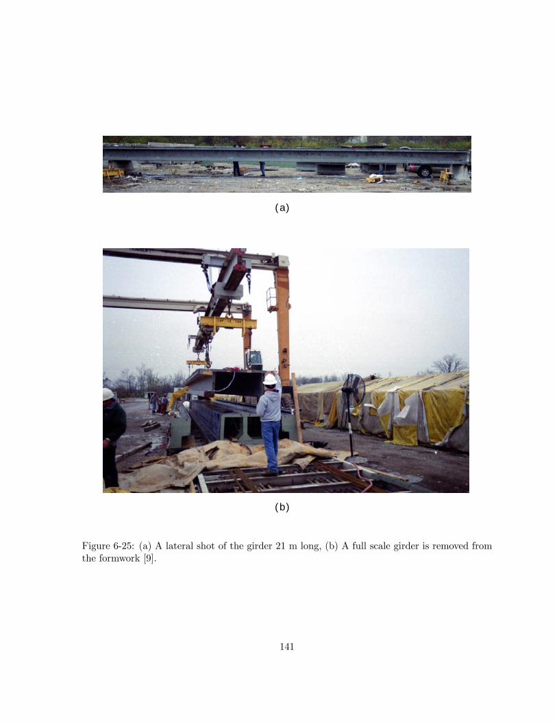
(a)
(b)
Figure 6-25: (a) A lateral shot of the girder 21 m long, (b) A full scale girder is removed fromthe formwork [9].
141

epsilon_(M,zz) on Deck
-1.0E-05
0.0E+00
1.0E-05
2.0E-05
3.0E-05
4.0E-05
5.0E-05
0.0 0.2 0.4 0.6 0.8 1.0 1.2
Width of Deck [m]
Pla
stic
Str
ain
[1
]
If applying prestress at 65 hours
If applying prestress at 120 hours
Before applying prestress
Figure 6-26: Comparison of the longitudinal plastic strains in the composite matrix along thedeck.
142

Beside the moment of prestress application, there are two more main factors which influence
the risk of early-age cracking in the considered UHPC bridge girder: autogenous shrinkage and
thermal deformation. While the autogenous shrinkage is a material property which cannot be
controlled once the material for the structure has been chosen, the thermal deformation can
be reduced by maintaining the structure in an isothermal temperature condition. During the
casting of the bridge girder, the external temperature varied between 0 C and 30 C so that
this temperature variation may affect the early-age cracking. Thus, it is also important to take
care of the external thermal condition in order to reduce early-age UHPC cracking.
6.6 Chapter Summary
We have raised the question whether it was possible to predict the risk of cracking in early-age
UHPC structures, and eventually reduce it - by means of the first-order engineering model
developed in this research. The application of the model to evaluate stresses and deformation
in the FHWA-UHPC bridge girders provides evidence that it is possible:
• To predict the temperature history and the strain history occurring in the UHPC bridge
girders.
• To evaluate the risk of cracking which is quantified in terms of plastic strains of the
composite matrix.
This was achieved by means of a first-order engineering model for early-age UHPC materials,
which is characterized by a relative small number of input parameters which can be accessed in
a rational manner. No doubt, the chosen modeling approach is strongly reductionist, reducing
the complex chemical reactions and phenomena that occur in UHPC materials to some very
few governing phenomena that are captured by the two-phase thermo-chemo-mechanical UHPC
material model, namely:
• The effect of hydration through a single hydration degree, whose evolution is monitored
through a macroscopic kinetics law.
143

• The effect of cracking through a permanent strain associated with the cementitious com-
posite matrix, whose evolution is monitored through strength criteria that depend on the
hydration degree.
• The coupling between hydration reaction, temperature and deformation, which are moni-
tored through a highly reduced number of input parameters, that are easily accessible for
the engineering practice.
The implementation of the model in a finite element program turns out to be a versatile
engineering tool to model the casting of UHPC structures, that allows engineers to predict and
reduce the risk of cracking.
144

Part IV
CONCLUSIONS
145

Chapter 7
CONCLUSIONS
7.1 Summary of Report
UHPC has remarkable performance in mechanical properties, ductility, economical benefit, etc.
However, early-age cracking of UHPC can become an issue during the manufacturing process
due to its intrinsic characteristics: the high cement content and the highly exothermic hydration
reaction. For this reason, there is a necessity to develop a material model which captures the
behavior of UHPC at early ages.
The objective of this research is to develop a new material model for early-age UHPC
through a thermodynamics approach. The new model is a two-phase thermo-chemo-mechanical
model, which is based on two pillars. The first is a hardened two-phase UHPC material model,
and the second is a hydration kinetics model for ordinary concrete.
Before developing the new model, these two theories are reviewed in detail. In the hardened
UHPC material model, the matrix and the fiber phases are modeled as two separate macroscopic
phases having the same macroscopic strain but different stress states for each phase. The
macroscopic model is composed of three parts: a brittle-plastic matrix phase, an elasto-plastic
fiber phase and an elastic coupling spring. An abrupt stress drop after the matrix cracking is
captured by this macroscopic model, and the plastic strain in the composite matrix represents
the cracking of UHPC. This hardened UHPC model is combined with a hydration kinetics
model which is based on the application of a decoupling hypothesis which neglects the effect of
mechanical change on the thermal and the chemical processes.
146

It is on the basis of these two models that we propose a new constitutive model for early-age
UHPC which combines the two-phase hardened UHPCmodel with the hydration kinetics model.
The coupling of these two model is achieved by considering the evolution of the strength and
stiffness properties in the two-phase UHPC material model. As a first engineering approach,
a linear evolution law is adopted for strength, and stiffness is assumed to follow a nonlinear
evolution law. This new two-phase thermo-chemo-mechanical coupling model is implemented
in a commercial finite element program, CESAR-LCPC. Finite element formulation including
finite element equations and the return mapping algorithm are presented in detail, and the
proposed model is verified through simulations of uniaxial tension tests.
The efficiency of the model and finite element program is validated with experimental data
obtained during the casting of a DuctalTM optimized bridge girder. Thanks to the decoupling
hypothesis, the application of the early-age UHPC model can be carried out in a two-step
manner: first the thermo-chemical problem is solved, followed by solving the two-phase thermo-
chemo-mechanical problem. The main findings from this application can be summarized as
follows:
1. A simulated adiabatic temperature curve which plays a major role in the thermo-chemical
problem is obtained from the quasi-isothermal strength values measured on site. From
the simulated adiabatic temperature curve and the thermal boundary conditions, the
temperature distribution was successfully obtained using the thermo-chemical simulation
tool.
2. The distribution of cracks on the deck and the web was predicted with the new two-phase
thermo-chemo-mechanical coupling approach. This simulated deformation behavior of
the girder compares well with on-site strain measurements. Thanks to the model, the
observed crack pattern were explained.
3. The developed engineering tool was also employed to study means to reduce the risk of
UHPC cracking. It is recommended that the external thermal condition should be well
taken care of, and the moment of applying prestressing force should be delayed.
The most important contribution is the novel macroscopic model for early-age UHPC. By
using the two-phase early-age UHPC model, one can evaluate the risk of cracking during the
147

casting of UHPC structures, and eventually reduce the risk of early-age cracking. The imple-
mentation of this model in a finite element program provides a versatile engineering tool for
improving the manufacturing of UHPC structures.
7.2 Future Research
The suggested material model for early-age UHPC is limited in several aspects by simplifying
assumptions, which should be addressed in future research. This material model adopts simple
evolution laws (Laube’s law and Byfors’ law) for the evolving strength and stiffness with respect
to the macroscopic hydration degree. The macroscopic hydration degree concept is only a first
step towards a comprehensive materials-to-structural engineering design approach. Recent
progress in experimental micro-mechanics makes it possible to assess the elastic properties at
very fine scales and to upscale this elastic behavior to large scales by means of homogenization
methods [4]. Thus, the simple evolution law for strength and stiffness of the UHPC material
can be replaced by the micro-mechanical approach with the homogenization methods.
By using chemo-mechanics and micro-mechanics, a multi-scale hydration kinetics model
could be developed to describe the hydration degrees of four clinker phases, i.e. C3S, C2S, C3A
and C4AF . Such a multi-hydration degree approach would involve the activation energy of the
four main hydration reactions, which could largely improve the predictive capabilities of our
single hydration degree approach, in which we use one single activation energy. This multi-scale
hydration kinetic model can then be applied to the two-phase UHPC model proposed in this
research. The tasks can be summarized at the different length scales of cementitious materials
as follows:
• At a micro-mechanical level, a link needs to be established between the four fundamental
chemical hydration reactions and UHPC strength and stiffness properties.
• At the material level, the micro-thermo-chemo-mechanical behavior could be upscaled
into a suitable macroscopic UHPC material model.
• At the structural level, such an improved model could examine how UHPC structures
must be optimized to minimize the risk of early-age UHPC cracking.
148

Ultimately, it would then be possible to make the link between mix proportion and structural
performance, and optimize the mix design for specific structural performances. The work
presented here is a first step towards this goal.
149

Bibliography
[1] Acker, Paul. (2004). Personal Communication.
[2] Bathe, K.J. (1996). Finite Element Procedures, Prentice-Hall, Upper Saddle River, New
Jersey.
[3] Bentur, A. (2003). "Early Age Cracking in Cementitious Systems", Report of RILEM
Technical Committee 181-EAS: Early age shrinkage induced stresses and cracking in ce-
mentitious systems, Bagneux, France.
[4] Bernard, O., Ulm F.J., and Lemarchand E. (2003). "A multiscale micromechanics-
hydration model for the early-age elastic properties of cement-based materials," Cement
and Concrete Research, September (9): 1293-1309.
[5] Boulay, C., Le Mau, F., Renwez, S., Sercombe, J., and Toutlemonde, F. (1997). "Car-
actérisation du comportement au choc d’un béton de poudres réactives grâce a des es-
sais de traction direct", Res Rep. LCPC-BOUYGUES, Laboratoire Central des Ponts et
Chaussées, Paris, France (in French).
[6] Byfors. (1980). "Plain Concrete at Early Ages," Swedish Cement and Concrete Institute,
Fo 3:80, Stockholm, Sweden.
[7] Chuang, E. (2002). "Ductility Enhancement of High Performance Cementitious Composites
and Structures," Ph.D. Dissertation, Massachusetts Institute of Technology, Cambridge,
Massachusetts.
[8] Chuang, E., and Ulm, F.-J. (2002). "Two-phase composite model for high performance
cementitious composites," Journal of Engineering Mechanics-ASCE, 128(12), 1314-1323.
150

[9] Geist, G. (2004). "MIT Optimized Ductal Bridge Girder Castings," Internal Document
from Lafarge.
[10] Heukamp, F.H, (2003). "Chemomechanics of calcium leaching of cement-based materials
at different scales: the role of CH-dissolution and C-S-H degradation on strength and
durability performance of materials and structures," Ph.D. Dissertation, Massachusetts
Institute of Technology, Cambridge, Massachusetts.
[11] Kupfer, H., Hilsdorf, H., and Rusch. (1969). "Behavior of concrete under biaxial stresses,"
ACI Journal, August, 656-666.
[12] Lafarge North America website. (2004). http://imagineductal.com
[13] Laplante, P. (1993). "Propriétés mécaniques des bétons durcissants: analyse comparée
des bétons classiques et à très hautes performances (Mechanical properties of hardening
concrete: a comparative analysis of ordinary and high performance concrete)," Ph.D. Dis-
sertation, Ecole Nationale des Ponts et Chaussées, Pararis, France (in French).
[14] Laube, M. (1990). "Werkstoffmodell zur berechnung won temperaturspannungen in mas-
sigen betonauteilen imm jungen alter," Docotral Thesis, TU Braunschweg.
[15] LCPC. (2004). "CESAR-LCPC Manual of Examples: Modeling of Early-Age UHPC,"
Laboratoire Central des Ponts et Chaussées, Paris, France.
[16] LCPC. (2001). "CESAR-LCPC Manual of Examples: Modeling of Early-Age Concrete,"
Laboratoire Central des Ponts et Chaussées, Paris, France.
[17] Neville, A.M. (1995). Properties of Concrete, Longman, Essex, England.
[18] Park, H. (2003). "Model-Based Optimization of Ultra High Performance Concrete Highway
Bridge Girders," M.S. Thesis, Massachusetts Institute of Technology, Cambridge, Massa-
chusetts.
[19] Perry, V.H. (2004). Personal Communication.
[20] Prestress Service Inc. (2003). Design Drawings of MIT Optimized Ductal Bridge Girder.
151

[21] Shim, J.M., and Ulm, F.J. (2004). "3-D Design Simulation and Validation of UHPC Model:
The Shawnessy Architectural Structure," MIT CEE Report R04-09, Massachusetts Insti-
tute of Technology, Cambridge, Massachusetts.
[22] Simo, J., and Hughes, T. (1997). Computational Inelasticity, Springer-Verlag, New York.
[23] Tennis, P.D., and Jennings, H.M. (2000). "A Model for Two Types of Calcium Silicate Hy-
drate in the Microstructure of Portland Cement Pastes," Cement and Concrete Research,
30, 855-863
[24] Ulm, F.J., and Coussy, O. (2002). Mechanics and Durability of Solids, Volume I: Solids
Mechanics, Prentice-Hall, Upper Saddle River, New Jersey.
[25] Ulm, F.J., and Coussy, O. (1995). "Modeling of Thermochemomechanical Couplings of
Concrete at Early Ages," Journal of Engineering Mechanics, July, 785-794.
[26] Ulm, F.J., and Coussy, O. (1996). "Strength Growth as Chemo-Plastic Hardening in Early
Age Concrete," Journal of Engineering Mechanics, December, 1123-1132.
[27] Ulm, F.J., and Coussy, O. (2001). "What Is a Massive Concrete Structure at Early Ages?:
Some Dimensional Arguments," Journal of Engineering Mechanics, May, 512-522.
152

Appendix A
Plastic Projection Schemes For
Triaxial Loading
• Projection Scheme for the Tension Cut-Off Condition:
∆λTCM =Itr1,M − σcrMt
9 (KM +KI)(A.1)
∆λTCF =Itr1,F − σFt
9 (KF +KI)(A.2)
• Projection Scheme for the Drucker-Prager Condition:
∆λUNM =αUNM Itr1,M +
¯strM¯− cUNM
2 (GM +GI) + 9¡αUNM
¢2(KM +KI)
(A.3)
∆λBIM =αBIM Itr1,M +
¯strM¯− cBIM
2 (GM +GI) + 9¡αBIM
¢2(KM +KI)
(A.4)
∆λDPF =
αDPF Itr1,F +
¯strF¯− cDP
F
2 (GF +GI) + 9¡αDPF
¢2(KF +KI)
(A.5)
153

• Projection Scheme for the Multiple Plastic Surface Condition:
⎧⎪⎪⎪⎪⎪⎪⎪⎪⎪⎨⎪⎪⎪⎪⎪⎪⎪⎪⎪⎩
∆λTCM
∆λTCF
∆λUNM
∆λBIM
∆λDPF
⎫⎪⎪⎪⎪⎪⎪⎪⎪⎪⎬⎪⎪⎪⎪⎪⎪⎪⎪⎪⎭= [A]−1
⎧⎪⎪⎪⎪⎪⎪⎪⎪⎪⎪⎨⎪⎪⎪⎪⎪⎪⎪⎪⎪⎪⎩
Itr1,M − σcrMt
Itr1,F − σFt
αUNM Itr1,M +¯strM + 2GI∆λDP,q
F Nup,qsF
¯− cUNM
αBIM Itr1,M +¯strM + 2GI∆λDP,q
F Nup,qsF
¯− cBIM
αDPF Itr1,F +
¯strF + 2GI
³∆λUN,q
M +∆λBI,qM
´Nup,qsM
¯− cDP
F
⎫⎪⎪⎪⎪⎪⎪⎪⎪⎪⎪⎬⎪⎪⎪⎪⎪⎪⎪⎪⎪⎪⎭(A.6)
where [A] is the following 5× 5 symmetric matrix:
[A] =
⎡⎢⎢⎢⎢⎢⎢⎢⎢⎢⎣
A11 A12 A13 A14 A15
A22 A23 A24 A25
A33 A34 A35
A44 A45
sym. A55
⎤⎥⎥⎥⎥⎥⎥⎥⎥⎥⎦(A.7)
where:A11 = 9 (KM +KI) ; A12 = −9KI ;
A13 = 9αUNM (KM +KI) ; A14 = 9α
BIM (KM +KI) ;
A15 = −9αDPF KI ;
A22 = 9 (KF +KI) ; A23 = −9αUNM KI ;
A24 = −9αBIM KI ; A25 = 9αDPF (KF +KI)
A33 = 2 (GM +GI) + 9¡αUNM
¢2(KM +KI) ;
A34 = 2 (GM +GI) + 9αUNM αBIM (KM +KI) ;
A35 = −9αUNM αDPF KI
A44 = 2 (GM +GI) + 9¡αBIM
¢2(KM +KI) ;
A45 = −9αBIM αDPF KI
A55 = 2 (GF +GI) + 9¡αDPF
¢2(KF +KI)
(A.8)
154

Appendix B
Input Format for EAHC Module
In CESAR-LCPC, running the EAHC module for the analysis of early-age UHPC reduces
to using a new material model. The EAHC module follows the regular input format of
CESAR-LCPC, except for the material input parameter. The new material model is assigned
IMOD = 119, which indicates early-age UHPC for the analysis of the two-phase thermo-
chemo-mechanical problem. Several examples which use the proposed material are presented
in Reference [15], and Table B.1 provide details for each model parameter of the early-age
UHPC model. Furthermore, input parameters and comments for MEXO simulation with
plane-section option are presented Table B.2. This is followed by the input files used in the
four-phase simulations with TEXO and MEXO. The description of the files is as follows:
TEXO
Simulation
⎧⎪⎪⎪⎪⎪⎪⎨⎪⎪⎪⎪⎪⎪⎩
Phase 1: grd_txp1.data
Phase 2: grd_txp2.data
Phase 3: grd_txp3.data
Phase 4: grd_txp4.data
MEXO
Simulation
⎧⎪⎪⎪⎪⎪⎪⎨⎪⎪⎪⎪⎪⎪⎩
Phase 1: grd_ehp1.data
Phase 2: grd_ehp2.data
Phase 3: grd_ehp3.data
Phase 4: grd_ehp4.data
155

Input Data Comments
TitleT itle = name of element group
IMOD (INAT )IMOD = control variable for the calculation;
IMOD=119 for early-age UHPC(INAT ) = only for 2-D problem
ρg ν CM CF Mρg = volumetric weightν = Poisson’s ratioCM = stiffness contribution of composite matrix in [MPa]CF = stiffness contribution of composite fiber in [MPa]M = stiffness of matrix-fiber coupling in[MPa]
σMt σcrMt σMc σMb
σMt = initial tensile strength of composite matrix in [MPa]σcrMt = post-cracking tensile yield strength of composite
matrix [MPa]σMc = initial compressive strength of composite matrix
in [MPa]σMb = initial biaxial compressive strength of composite
matrix in [MPa]
σFt σFcσFt = tensile strength of composite fiber in [MPa]σFc = compressive strength of composite fiber in [MPa]
αM −βM ξ0 ξinitial
αM = thermal dilatation coefficient of composite matrixβM = autogenous shrinkage for composite matrixξ0 = threshold of the hardened composite matrixξinitial = initial hydration degree indicating whether the
group is chemically active or not; ξinitial=1 forhardened UHPC and ξinitial=0 for early-ageUHPC
αF −βFαF = thermal dilatation coefficient of composite fiberβF = autogenous shrinkage for composite fiber; for
steel fiber βF=0
Table B.1: Input parameters and comments for the early-age UHPC model, IMOD = 119.These input parameters are introduced under ELEM in the MEXO input files.
156

Input Data Comments
MEXOMNPAS1
MEXO = computation module for thermo-chemo-mechanical calculationM = print index;M=0 for printout of the number of time stepsM=1 for printout of M=0 plus functions influencing the parameter
and loading functionsM=2 for printout of the solution at each time stepM=4 for printout of the the stresses at each time step
NPAS1=number of time steps of the TEXO computation used for theMEXO computation
TXOM0NOMF
TXO = input of the temperature fields and degree of hydration fromthe TEXO computation results files; if TXO is not specifiedthen calculation become hardened UHPC simulation.
M0 = selection indicator of the time steps stored by TEXO;M0=0 if all of the time steps from the TEXO computation are used.M0=1 otherwise
NOMF = name of the results file created by the TEXO module
ININOMF
INI = initialization of a computation by input from a restart fileNOMF = name of the restart file
STKNOMF
STK = storage of results at the last time step for a subsequentcomputation restart
NOMF = name of the file on which the results of the last timestep are stored
EFNIEPTXC, Y CV NM0[3]V NM1[3]...V NMNPAS1[3]
EFN = plane-section computationIEPT = print index;IEPT=1 for an unspecified sectionIEPT=2 for a section having y-axis as a symmetric axisIEPT=3 for a section having x -axis as a symmetric axisIEPT=4 for a section having x - and y-axis as symmetric axes
XC, Y C = symmetric axis coordinate if IEPT having 2, 3 or 4
V NM IPAS [3] = Nd, Mdx, M
dy = prescribed force and moments,
which follow the sign conventions in Section 6.3
NITIMETNITERTOL
NIT = convergence criteria for nonlinear calculationIMET =1 for default convergence checking algorithm in CESARNITER = maximum number of iterationTOL = tolerance for convergence
Table B.2: Input parameters and comments for MEXO simulation with plane-section option,EFN .
157