doi.org/10.26434/chemrxiv.14411081.v1

Prediction and Optimization of Ion Transport Characteristics inNanoparticle-Based Electrolytes Using Convolutional Neural NetworksSanket Kadulkar, Michael Howard, Thomas Truskett, Venkat Ganesan

Submitted date: 14/04/2021 • Posted date: 15/04/2021Licence: CC BY 4.0Citation information: Kadulkar, Sanket; Howard, Michael; Truskett, Thomas; Ganesan, Venkat (2021):Prediction and Optimization of Ion Transport Characteristics in Nanoparticle-Based Electrolytes UsingConvolutional Neural Networks. ChemRxiv. Preprint. https://doi.org/10.26434/chemrxiv.14411081.v1

We develop a convolutional neural network (CNN) model to predict the diffusivity of cations innanoparticle-based electrolytes, and use it to identify the characteristics of morphologies which exhibit optimaltransport properties. The ground truth data is obtained from kinetic Monte Carlo (kMC) simulations of cationtransport parameterized using a multiscale modeling strategy. We implement deep learning approaches toquantitatively link the diffusivity of cations to the spatial arrangement of the nanoparticles. We then integratethe trained CNN model with a topology optimization algorithm for accelerated discovery of nanoparticlemorphologies that exhibit optimal cation diffusivities at a specified nanoparticle loading, and we investigate theability of the CNN model to quantitatively account for the influence of interparticle spatial correlations on cationdiffusivity. Finally, using data-driven approaches, we explore how simple descriptors of nanoparticlemorphology correlate with cation diffusivity, thus providing a physical rationale for the observed optimalmicrostructures. The results of this study highlight the capability of CNNs to serve as surrogate models forstructure--property relationships in composites with monodisperse spherical particles, which can in turn beused with inverse methods to discover morphologies that produce optimal target properties.

File list (2)

download fileview on ChemRxivPrediction and optimization of ion transport characteristics ... (5.51 MiB)

download fileview on ChemRxivSupplementary Information.pdf (2.33 MiB)

Prediction and optimization of ion transport

characteristics in nanoparticle-based electrolytes

using convolutional neural networks

Sanket Kadulkar,† Michael P. Howard,† Thomas M. Truskett,∗,‡ and Venkat

Ganesan∗,†

†McKetta Department of Chemical Engineering, University of Texas at Austin, Austin,

Texas 78712, USA

‡McKetta Department of Chemical Engineering and Department of Physics, University of

Texas at Austin, Austin, Texas 78712, USA

E-mail: truskett@che.utexas.edu; venkat@che.utexas.edu

1

Abstract

We develop a convolutional neural network (CNN) model to predict the diffusivity

of cations in nanoparticle-based electrolytes, and use it to identify the characteristics of

morphologies which exhibit optimal transport properties. The ground truth data is ob-

tained from kinetic Monte Carlo (kMC) simulations of cation transport parameterized

using a multiscale modeling strategy. We implement deep learning approaches to quan-

titatively link the diffusivity of cations to the spatial arrangement of the nanoparticles.

We then integrate the trained CNN model with a topology optimization algorithm for

accelerated discovery of nanoparticle morphologies that exhibit optimal cation diffu-

sivities at a specified nanoparticle loading, and we investigate the ability of the CNN

model to quantitatively account for the influence of interparticle spatial correlations

on cation diffusivity. Finally, using data-driven approaches, we explore how simple

descriptors of nanoparticle morphology correlate with cation diffusivity, thus providing

a physical rationale for the observed optimal microstructures. The results of this study

highlight the capability of CNNs to serve as surrogate models for structure–property

relationships in composites with monodisperse spherical particles, which can in turn

be used with inverse methods to discover morphologies that produce optimal target

properties.

1 INTRODUCTION

Nanocomposites comprising spherical nanoparticles dispersed in polymeric matrices or liquid

hosts have emerged as a promising class of materials for a broad range of applications. The

introduction of nanoparticles can enhance the ionic conductivity,1,2 mechanical strength,3–5

optoelectronic properties,6,7 and separation performance8–10 of the host material. Since the

mechanisms underlying the observed property improvements remain poorly understood,11,12

there is interest to find new approaches to predict the nanoparticle loading and microstruc-

ture characteristics that optimizes the properties of interest.

2

Although nanoparticle loading is known to be an important factor influencing nancom-

posite properties, experimental and theoretical studies have found that the spatial orga-

nization of the nanoparticles also strongly influences macroscopic behavior. For instance,

Jana and coworkers reported polybenzimidazole nanocomposite systems with morphology-

dependent proton conduction13–15 and storage modulus14 properties at a fixed nanoparticle

loading. In their studies, the characteristic structure of the dispersed nanoparticles was

altered by modifying the nanoparticle surface with various functional groups. Similarly, Ak-

cora et al. 16 reported tunability in mechanical properties of polymer nanocomposites at a

fixed nanoparticle volume fraction by varying the grafting density and molecular weight of

tethered chains, and attributed such behavior to the resulting modulation of the nanoparti-

cles’ self-assembled structure. A recent mesoscale simulation study of ours17 highlighted the

potential for modifying nanoparticles structure to significantly influence the tracer diffusivity

through nanocomposite gels in the presence of interface-assisted transport pathways.

A key challenge in any of these efforts is to determine specific nanoparticle microstructures

that are optimal for targeted macroscopic properties. Knowledge of such microstructures

could provide new mechanistic insights, and in addition facilitate discovery of nanoparticle

interactions that are most promising for experimental realization of the microstructures using

inverse methods.18,19 Due to the high-dimensional nature of the relevant search spaces, which

in principle includes all possible configurations of the nanoparticles, experimental screening

of candidate microstructures is often practically intractable. An attractive alternative is

to solve for the microstructures using a topology optimization algorithm20–23 that leverages

structure–property predictions from a computationally tractable surrogate model.

In this context, data-driven models have recently emerged as a promising approach for

quantifying the structure–property relationships in two-phase composites. Specifically, ma-

chine learning approaches have been employed to develop surrogate models for quantitative

prediction of macroscopic properties with binary composite microstructure as input, rep-

resented by either low-dimensional structural descriptors or as representative volume ele-

3

ments. In the studies pertaining to the former, the hand-crafted features representing the

microstructure are linked to an associated property using a regression-based model24–30 or

artificial neural network.31,32 For the latter case, convolutional neural networks (CNNs)33 are

employed to extract important features from the digitized images of composite microstruc-

tures, generated by stochastic growth of grains34–38 or by random assignment of numbers in

the uniformly voxelized grids,39–41 in order to predict the effective property of interest.

Motivated by the above advances, we hypothesize that machine learning techniques can

be similarly applied to correlate the properties of nanocomposites reinforced with spherical

nanoparticles to their microstructure. Further, integrating such structure–property linkages

with microstructure optimization algorithms could significantly accelerate the exploration

of the relevant high-dimensional configuration spaces to identify nanoparticle morphologies

possessing optimal characteristics.

In this study, we demonstrate the above strategy by the application of deep learn-

ing approaches for predicting the diffusion coefficient of cations in single-ion conducting

nanoparticle-based electrolytes. The choice of the system was inspired by a recent study

of ours42 probing the mechanistic bases for ion transport observations reported in these

electrolytes. Our results in such a context were consistent with the reported experimental

behavior of electrolytes comprising silica nanoparticles, cofunctionalized with polyethylene

glycol ligands and tethered anionic species coupled to Li+ ions, dispersed in ion-conducting

tetraglyme solvent.43,44 Our simulation results suggested that ionic conductivity in such sys-

tems is primarily controlled by cation diffusion along functionalized nanoparticle surfaces.

With such mechanistic findings, the connectivity of the cation diffusion pathways is hypoth-

esized to be dependent on the spatial arrangement of the nanoparticles, and it would be

desirable to identify the morphologlies that exhibit optimal cation diffusivities.

In this work, we develop a three-dimensional (3D) CNN model to capture the nonlin-

ear mapping between the nanoparticle microstructure and the resulting cation diffusivity.

The structure–property linkages established using the CNN model exhibit better accuracy

4

for predicting diffusivities compared to that using other deep learning models based on

physics-inspired approaches. We then use the trained CNN model to perform topology op-

timization for identifying nanoparticle configurations that can potentially exhibit a wider

range of diffusivities. We explore the extent to which the deep learning model captures the

relevant physical information influencing cation diffusivity based on the CNN predictions

for microstructures with different nanoparticle volume fractions. Lastly, by analyzing the

influence of physics-inspired structural descriptors on cation diffusivity, we discuss the struc-

tural characteristics of the optimal microstructures and provide a physical rationale for the

optimal cation diffusivities exhibited by these structures. While the present study is inspired

by the nanoparticle-based electrolyte system, the methods and ideas presented in this work

can be easily adapted to establish quantitative structure–property relationships and identify

optimal morphologies in other nanoparticle-based systems.

The rest of the article is organized as follows. Details of the dataset generation, training of

the CNN model, and topology optimization algorithm are provided in Section 2. The results

pertaining to the predictive performance of the model, and its ability to discover optimal

microstructures when integrated with a topology optimization algorithm, are presented in

Section 3. By modifying the inputs to the CNN model, we provide a physical interpretation

of its learning aspects in Section 4. We report on the correlation of physics-inspired structural

descriptors with cation diffusivity using the data-driven approaches in Section 5. Section 6

concludes the paper with a summary of our findings and provides an outlook regarding

the generality of our methodology to train CNN models for exploring structure–property

relationship in two-phase composites doped with spherical nanoparticles.

2 DATASETS AND METHODS

Figure 1 illustrates the workflow implemented in this study. In this section, we discuss the

methodologies adopted to generate the training dataset, train the CNN-based deep learning

5

Figure 1: Flowchart for CNN-assisted prediction and optimization of cation diffusivity innanoparticle-based electrolytes.

model, and integrate the CNN model with the topology optimization algorithm for prediction

and optimization of cation diffusivity in nanoparticle-based electrolytes.

The ground truth data used in the training process is generated via a multiscale sim-

ulation framework which computes the cation diffusivities for a large dataset of diverse

microstructures at a fixed nanoparticle loading. Section 2.1 describes the physics-inspired

strategy employed to generate the dataset of diverse microstructures at a fixed nanoparticle

loading to span a wide range of cation diffusivities for training the machine learning mod-

els. Section 2.2 discusses the methodology to compute ground truth cation diffusivity for a

given nanoparticle microstructure. The details pertaining to the CNN architecture and the

topology optimization runs are presented in Section 2.3 and Section 2.4, respectively. An

improved predictive model is developed by appending the structures identified using the op-

timization strategy (as well as the corresponding simulated cation diffusivities) to the initial

training dataset, and subsequently retraining the CNN model as discussed in Section 2.5.

6

2.1 Generation of Microstructure Dataset

Training a CNN model to predict the diffusivity of cations in nanoparticle-based electrolytes

requires generating a large dataset of diverse nanoparticle topologies exhibiting a wide range

of cation diffusivities. The dataset itself includes thousands of configurations of nanoparti-

cles, represented in the form of 3D digitized images, and the values of the associated cation

diffusivities, calculated using the mesoscale kMC simulations discussed in Section 2.2.

The number of nanoparticles considered for the microstructures in the dataset should be

large enough to capture the wide variety of possible topologies spanning length scales relevant

for cation transport. At the same time, the microstructures should be small enough such that

the ground truth diffusivities for a large number of distinct particle configurations can be

calculated at a reasonable computational cost. In our study, we balance these considerations

by using configurations of N = 91 identical nonoverlapping nanoparticles of diameter σNP in

a cubic box of size L with periodic boundary conditions. The nanoparticle volume fraction

Nπσ3NP/(6L

3) is fixed to be 0.1 for all the structures. Such a choice of volume fraction

allows for realizing a variety of nanoparticle configurations exhibiting broad range of cation

diffusivities.

To achieve high prediction accuracy for a wide variety of morphologies in the configura-

tional space screened during the topology optimization runs, a large training dataset contain-

ing diverse microstructures and large variation of cation diffusivities is required. However,

only a relatively narrow distribution of cation diffusivities was obtained for the configura-

tions generated using random sequential adsorption (RSA) algorithm45 (supporting results

in SI, Section S2) which ensures nonoverlap between nanoparticles in the microstructure.

Accordingly, we modify the standard RSA algorithm with the addition of physics-based

modifications described below to ensure that configurations corresponding to a wide range

of cation diffusivities are included.

For the ion transport model considered here, we previously reported42 that the average

nearest particle distance and percolation of the nanoparticles are significant aspects influenc-

7

ing diffusivity. Briefly, the former dictates the “connectivity” between adjacent nanoparticles

and correspondingly the mobility of cations while hopping from the surface of a nanoparticle

to that of its neighbor. In the model, there exists an ideal range for the distance between ad-

jacent particles to facilitate cation transport; separations too large disrupt “contact” between

neighboring nanoparticle surface regions and separations too close result in interdigitation of

nanoparticle surface functional groups that reduces cation mobility. Percolation, which char-

acterizes the spatial extent of particle connectivity and thereby the corresponding surface

transport pathways, correlates positively with cation diffusivity.

Given these physical considerations, we modify the standard RSA algorithm to generate

different microstructures that represent a wide range of average nearest particle distances and

extents of percolation. Specifically, we generate 5304 structures by randomly inserting each

new particle within a specified range of distances from the previous particle (In SI, Section

S2 we present more details on what different constraint distances were used). 2166 additional

configurations were generated using RSA algorithm with a further constraint that explicitly

disrupted percolation in one or more dimensions of the simulation box (more details in SI,

Section S2). The dataset also includes 722 structures generated using an RSA algorithm

with no constraints. The configuration data is then split randomly into training, validation

and test datasets with 4916, 1638, and 1638 microstructures, respectively.

2.2 Model and Simulation Methodology to generate ground truth

Labels for Microstructures

Since simulation of nanoparticle-based electrolytes using atomistically detailed molecular

models is computationally prohibitive, we use the multiscale simulation framework from our

recent study42 to compute the cation diffusivities for microstructures in the training dataset.

In brief, this multiscale simulation strategy involves using coarse-grained molecular dy-

namics (MD) simulations to probe the region between two adjacent functionalized nanopar-

ticles. Such simulations provide means for characterizing the effective pair interactions be-

8

tween functionalized nanoparticles, as well as the spatial distribution of the cations and their

local (i.e., position-dependent) diffusivity. This information serves as input for an on-lattice,

mesoscale model of the nanoparticle-based electrolyte in which kinetic Monte Carlo (kMC)

simulations are used to simulate transport of cations through the given nanoparticle config-

uration. The bulk diffusivity of cations DkMC is then calculated from the resulting cation

trajectories using the Einstein–Smoluchowski relation,

DkMC = limt→∞

1

6t〈[ri(t)− ri(0)]2〉, (1)

where 〈[ri(t)− ri(0)]2〉 is the mean squared displacement of cations at time t.

Due to the large separation of time scales between diffusion of cations and nanoparticles,

the nanoparticles are treated as immobile obstacles in the simulations. Further details about

the coarse-grained MD and mesoscale kMC simulations are provided in the SI, Section S1.

In the present work, cation diffusion coefficients computed for the microstructures in

the training dataset using kMC simulations parameterized with a fixed set of cation local

diffusivities and cation-nanoparticle affinities, determined from the coarse-grained MD sim-

ulations of our previous study,42 serve as the ground truth labels. To emphasize the efficacy

of employing the combination of CNN model and topology optimization algorithm to iden-

tify non-intuitive microstructures with high diffusivities, we define a dimensionless number,

D∗kMC = DkMC/Do, where Do is the maximum value of ground truth cation diffusivity in the

originally generated dataset.

2.3 Convolutional Neural Network Model

The convolutional neural network (CNN) is a widely-used deep learning approach for com-

puter vision tasks,46 which utilizes image-like data as input. A typical CNN architecture

includes the following different layers: convolutional layers, pooling layers, activation func-

tions and fully connected layers. Convolutional layers extract the spatial features of the

9

Figure 2: Architecture of the 3D CNN.

input image by applying filters learned from the training dataset. An activation function

is usually applied after the convolutional layer to introduce nonlinearity into the network

and capture the complex relationship between the inputs and outputs. Pooling layers are

added after the activation functions to reduce the dimensions of the feature map outputs

from the convolutional layer. Finally, the objective of the fully connected layers is to predict

the output value based on the nonlinear combinations of the feature maps from a series of

convolution and pooling layers.

The resolution of the CNN input in every direction was chosen to be 5 times lower than

the grid size adopted for the on-lattice kMC simulations. Such a resolution sufficiently

mitigates discretization effects while maintaining a small enough input size to the CNN

models for computational efficiency. Accordingly, all microstructures are first converted to

a 75 × 75 × 75 binary images, where voxels corresponding to the region occupied by the

nanoparticles are denoted as 1, and 0 is used to index the empty voxels (more details in SI,

Section S3). Although the on-lattice kMC simulation models cation transport through the

nanoparticle microstructure using periodic boundary conditions, the convolutional layers

in the CNN are incapable of capturing the periodic boundary conditions on the spatial

volume unless the input image explicitly reflects the periodicity. Since the relevant length

scales influencing the transport of cations are typically larger than the dimensions of the

nanoparticle microstructure considered in this study, every binary image constructed from

the nanoparticle configuration in the cubic box is repeated 3 times in all three directions,

and the resulting binary image of size 225 × 225 × 225 is provided as input to the CNN

10

model to better capture the effect of periodic boundary conditions. (Results for the inferior

CNN model performance without the repetition of binary image are presented in SI, Section

S5.1).

The diameter of a single nanoparticle is approximately the length of 10 voxels in the input

image, and convolutional filters of size comparable to multiple nanoparticles are needed to

capture interparticle spatial correlations. Convolutional layers with such large filter size

also require a relatively large number of filters to effectively account for spatial features

incorporating multiple nanoparticles. However, the training process of such CNN models

with large datasets is computationally intractable. Instead, we employ a deeper network

comprising multiple layers while choosing the convolutional filter size for every layer to be

smaller than that of a single nanoparticle, as illustrated in Figure 2. We fix the convolutional

filter size to be 3 × 3 × 3 for all the layers. The CNN architecture considered for this study

consists of four composite layers, each consisting of a convolution layer, a rectified linear

unit (ReLU) activation function, and average pooling layer, followed by two fully connected

layers. The number of convolutional filters and neurons in the fully connected layers were

decided based on the accuracy of testing set predictions for the respective CNN architectures

(results for different CNN architectures presented in SI, Section S5.2).

The CNN models were trained on 4 NVIDIA Tesla V100 GPUs with 16GB RAM for each

GPU, using the Keras library47 built on top of Tensorflow implemented in Python 3.7. The

hyperparameters used to train the CNN models are reported in SI, Section S4.

2.4 Topology Optimization using Simulated Annealing

Simulated annealing (SA) is an effective, heuristic algorithm that stochastically searches for

the global optimum of an objective function on a landscape where many local optima may be

present. The approach has analogies to physical annealing, where a material avoids getting

trapped in local energy minima (e.g., defective crystals or glasses) and eventually realizes

its lowest energy state (i.e., crystal) by slowly cooling it from high to low temperature.

11

Earlier studies have utilized SA for solving structural optimization problems with discrete

variables.48–50 In this article, we integrate the trained CNN model with an SA algorithm

to navigate the morphological space and identify microstructures exhibiting a wide range of

diffusivities. From a design perspective, one may be interested in identifying structures with

high diffusivities. However, discovery of low-diffusivity microstructures is also essential for

progressively improving the CNN model through their incorporation in the training process

as discussed in Section 2.5. Toward these objectives, two independent SA algorithms were

employed to find microstructures that maximize (and minimize) the cation diffusivities,

naturally leading to the discovery of microstructures with higher (and lower) simulated

diffusivities than those for structures in the originally generated dataset.

At each step of the SA algorithm, the center of a nanoparticle is randomly moved to a

neighboring voxel in the binary image while ensuring nonoverlap of nanoparticles. When the

SA algorithm is used to maximize diffusivity, the probability of accepting the move/transition

from structure i to structure j (pij) is given by:

pij =

1, D∗CNN(j) ≥ D∗CNN(i)

exp[D∗

CNN(j)−D∗CNN(i)

D∗k

], D∗CNN(j) < D∗CNN(i),

(2)

where D∗CNN(j) is the diffusivity for structure j, estimated using the CNN model and nor-

malized by Do, and D∗k is a dimensionless control parameter chosen for the kth cycle of the

SA algorithm. A geometric cooling profile was adapted for D∗k, k = 2, 3, ...., kmax, described

by the formula:

D∗k = αD∗k−1 (3)

where α = 0.9 and D∗1 = 9.8 × 10−3. A similar condition as in Eq. 2 is applied to advance

the SA algorithm for minimizing diffusivity, except the diffusivities are replaced by their

negative values. The total number of cycles (kmax) in the SA algorithms used to maximize

and minimize diffusivity were 50 and 100, respectively. 2500 steps of the SA algorithm were

12

performed for each cycle. To ensure that microstructures from different domains of the struc-

tural landscape were screened, we performed 10 independent runs for both SA algorithms

with a different initial morphology for each run, generated using the RSA algorithm.

2.5 Retraining the CNN Model

Due to the limited microstructural domains featured in the dataset generated using the

methodology discussed in Section 2.1, augmenting the microstructures with those identified

from optimizing the CNN model with the SA algorithm, and subsequently retraining the

CNN model with the expanded dataset, is expected to improve diffusivity predictions for

a wider range of nanoparticle morphologies.51,52 To this end, cation diffusivities for the

structures identified from the topology optimization runs were calculated using our kMC

simulation methodology. Specifically, from the structures evaluated during the SA algorithm

for maximizing diffusivity, 5000 configurations with uniform distribution of CNN-predicted

diffusivities higher than the maximum diffusivity value in the original dataset were chosen

randomly, analyzed using the kMC simulations and added to the dataset. Similarly, 2280

structures from the ones explored using the SA algorithm for minimizing diffusivity were

evaluated using kMC simulation and appended to the dataset as well. The numbers of

training, validation and test data points for the new dataset were 9712, 3240, and 3240,

respectively. Following the retraining of the CNN model, the topology optimization process

described in Section 2.4 was repeated using the updated CNN model.

3 RESULTS AND DISCUSSION

3.1 CNN Model Performance

In this section, we present results demonstrating the ability of the CNN model to accurately

predict cation diffusivity values. The performance of the CNN model is compared with

other deep learning models based on physics-inspired approaches. The accuracy of a model

13

Figure 3: CNN predictions for original dataset. Parity plots of CNN model for (a) trainingand (b) testing sets.

is reported using the mean squared error (MSE) and mean absolute percentage error (MAPE)

which are defined as:

MSE =1

N

N∑i=1

(yi − yi)2 (4)

MAPE =1

N

N∑i=1

∣∣∣∣yi − yiyi

∣∣∣∣× 100% (5)

where yi is the value predicted by the model, and yi is the ground truth value.

Figure 3 shows a parity plot between the diffusivities predicted using the best-performing

CNN and those calculated using the kMC simulations. We observe that the CNN model

predicts the cation diffusivity for the unseen microstructures in the testing set with high ac-

curacy. Moreover, the trained CNN model predicts the cation diffusivity with computational

cost of roughly three orders magnitude lower than the kMC simulations.

Next, we compare the performance of the CNN model with other physics-inspired deep

learning models (Figure 4) created to establish quantitative structure–property linkages.

In the absence of a preexisting analytical model for predicting transport properties in

nanoparticle-based composites (for which nanoparticle-surface transport pathways have a

strong influence), artificial neural network models were trained with simple, structural de-

14

Figure 4: Schematic of the alternative physics-inspired deep-learning models using (a)average nearest particle distance or (b) particle-particle radial distribution function as mi-crostructural inputs to predict cation diffusivity.

scriptors as input features. In one of the methods, we use the average nearest particle

distance, reported to be a measure which correlates well with the cation diffusivity for the

ion transport model considered in this study.42 We also explored another surrogate model

with nanoparticle-nanoparticle radial distribution function as the input feature to predict

cation diffusivity. Although other two-point (particle-particle) correlation functions have

been employed as structural descriptors for predicting properties of composites with gran-

ular and continuous phases,24,31,32,53–59 we observe the radial distribution functions to be a

more relevant descriptor for the microstructures in our case with uniformly sized nanoparti-

cles (supporting results in SI, Section S6.2). Further details on the architecture of the deep

artificial neural networks adopted for the above physics-inspired approaches are provided in

SI, Section S6.1. The performance of such models is evaluated on the same training and

testing set generated using the methodology discussed in Section 2.1.

From the results displayed in Figure 5, the CNN model is able to furnish more accurate

predictions than the physics-inspired models. This suggests that the physics-based descrip-

tors, which do not contain information pertaining to many-body spatial correlations, may

be insufficient for identifying the most relevant microstructural features influencing cation

diffusivity. For the CNN model, although the convolutional filter size is smaller than the size

of a nanoparticle, the spatial correlations between multiple nanoparticles can be captured

by the deeper network implemented in this study with four convolutional layers.60,61 More

15

Figure 5: Bar graph for the MSE and MAPE of the predictive models for structures in theoriginally generated (a) training and (b) testing sets.

specifically, the CNN filters can effectively capture the relevant 3-point and higher-order

spatial correlations40 influencing transport in ways not possible from deep-learning models

based on the simpler physics-inspired descriptors.

The quantitative agreement between the CNN predictions and the ground truth diffusiv-

ities provides evidence that CNNs are a promising tool for predicting macroscopic properties

of two-phase composites comprising spherical nanoparticles. Further, since predicting dif-

fusivity using the CNN model is faster than running brute kMC simulations, it can be an

efficient proxy in frameworks that require many evaluations of cation diffusivity. We there-

fore integrate the CNN models with the topology optimization algorithms which requires

calculating cation diffusivity at each step, to help discover new composite materials with

desired characteristics and develop even more accurate predictive tools as discussed below.

16

Figure 6: Example of topology optimization using SA. (a) CNN-predicted diffusivity and (b)acceptance probability of a structural change at each SA cycle for diffusivity maximization.(c) CNN-predicted diffusivity and (d) acceptance probability of a structural change at eachSA cycle for diffusivity minimization. (e) Parity plot comparing diffusivity obtained viakMC simulation versus the CNN model for randomly chosen structures evaluated during thetopology optimizations.

17

3.2 Topology Optimization for Diffusivity using the CNN Model

Next, we explore the efficacy of using SA optimization with the CNN model to identify a

diverse array of microstructures with diffusivities outside the bounds of those observed for

structures in the originally generated dataset.

We show results pertaining to two of the 20 independent runs for the SA algorithms

used to find microstructures that maximize (or alternatively minimize) cation diffusivity as

discussed in Section 2.4. For the SA algorithm to maximize diffusivity, the CNN-predicted

diffusivities converge to an optimal value as shown in Figure 6a. From the results displayed

in Figure 6b, it is seen that the control parameter D∗k is changed slowly enough such that

the acceptance rate steadily decreases from an initial value of 1 to 0, indicating convergence

to the optimal solution. Similarly, the results presented in Figure 6c,d indicate converged

solution for the SA algorithm to minimize diffusivity.

Figure 6e shows the comparison between diffusivities predicted by the CNN model and

those computed using the kMC simulations for the randomly chosen structures evaluated dur-

ing the optimization process (as discussed in Section 2.5). It is apparent that, although these

diverse microstructures with a wide range of diffusivities were not included in the training

dataset, the CNN model estimates the diffusivity for such structures with reasonable accu-

racy. Furthermore, a Pearson’s R (as a measure of linear correlation)62 of 0.975 between the

CNN-predicted and ground truth diffusivities demonstrates the ability of the trained CNN

model to identify the relevant spatial features influencing diffusivity, and thereby successfully

progress towards optimal microstructures by integrating with SA algorithm.

3.3 Performance of Retrained CNN Model

In this section, we present results for the performance of the CNN model revised using the

expanded training dataset comprising the original dataset along with the microstructures

identified from the topology optimization runs with CNN-predicted diffusivities outside the

bounds of those in the originally generated dataset (as discussed in Section 2.5).

18

Figure 7: Predictions of retrained CNN model for expanded dataset. Parity plots comparingkMC and CNN-predicted diffusivity for (a) training and (b) testing sets. (c) Parity plotscomparing kMC and CNN-predicted diffusivity for randomly chosen structures evaluatedduring the topology optimization SA runs with the retrained CNN model.

Figure 7 shows parity plots comparing diffusivity computed from kMC simulations to

that predicted from the retrained CNN model. We observe excellent agreement with an

MSE/MAPE of 8.978 × 10−4 / 3.147% and 1.164 × 10−3 / 3.632% for structures in the

modified training and testing sets, respectively. We further report the model predictions for

the structures discovered on repeating the topology optimization runs using SA (as described

in Section 2.4) with the revised CNN model to estimate diffusivities. From the results shown

in Table 1, we observe improved accuracy with the revised CNN model for the structures

screened during the SA runs for topology optimization. Further, a Pearson’s R close to one

(R = 0.985) is observed between the predicted and ground truth values.

In the next section, we present results which explore the extent to which the CNN model

encodes information about the presence of nanoparticles by testing its ability to predict

cation diffusivities for microstructures with nanoparticle volume fractions lower and higher

than those in the training dataset.

Table 1: Comparison of prediction accuracy for structures evaluated during theSA algorithm runs

Model MSE/MAPECNN model trained with original dataset 3.611× 10−2 / 15.634%

CNN model retrained with expanded dataset 5.739× 10−3 / 7.133%

19

4 CNN Predictions for different Nanoparticle Load-

ings

The success of the CNN model studied here for predicting cation diffusivity in nanocom-

posites with spherical nanoparticles clearly hinges on its ability to detect how nanoparticle

positions and the related positional interparticle correlations influence diffusivity. Here, by

modifying the types of microstructures we input into the revised CNN model, we aim to

examine whether the CNN filters can adequately recognize and account for the impact of

added or deleted nanoparticles, and accordingly predict the corresponding cation diffusivity.

Based on the ion transport model considered in this study, the cation diffusivity is ex-

pected to be significantly influenced by the nanoparticle volume fraction.42 Since the effect

of nanoparticle volume fraction on the cation diffusivity was not explicitly introduced to the

CNN model during the training process, we interpret what the model learns by studying

the accuracy of the CNN model predictions for microstructures of different volume fractions.

To that end, nanoparticles were randomly added to (removed from) each structure in the

Figure 8: Predictions of retrained CNN model for different nanoparticle (NP) loadings.Parity plots comparing kMC and CNN-predicted diffusivity for microstructures with (a)15% NP loading and (b) 5% NP loading, by volume.

20

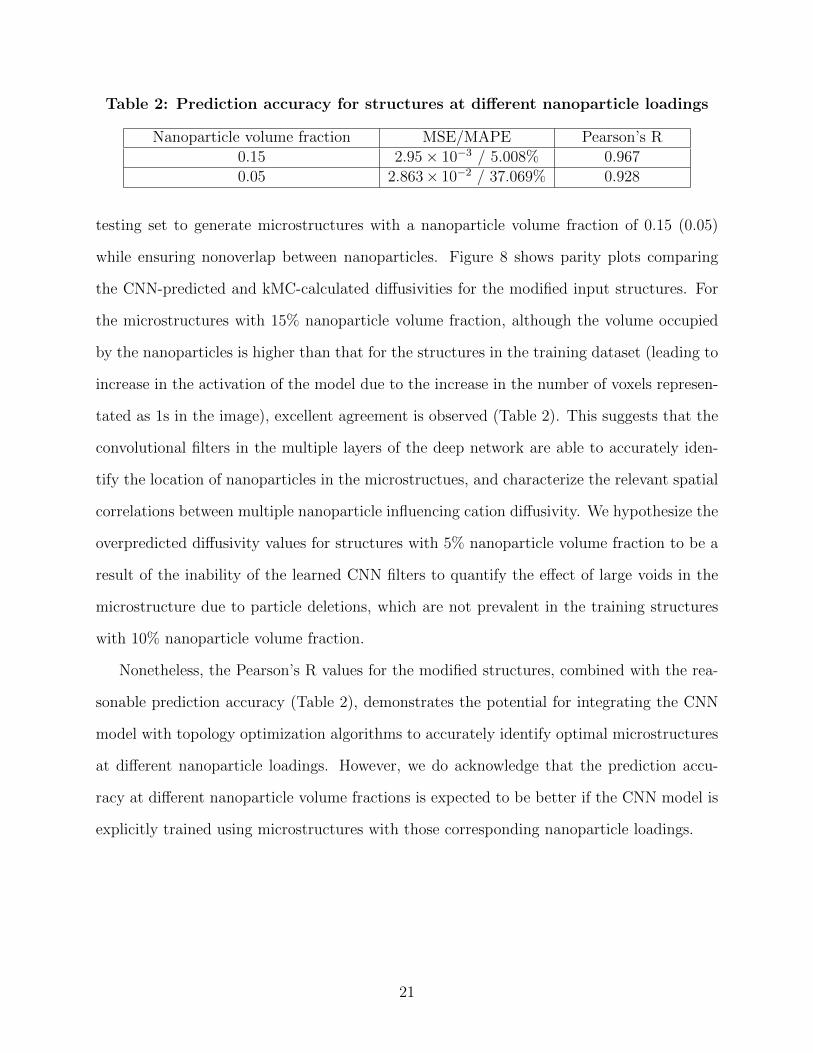
Table 2: Prediction accuracy for structures at different nanoparticle loadings

Nanoparticle volume fraction MSE/MAPE Pearson’s R0.15 2.95× 10−3 / 5.008% 0.9670.05 2.863× 10−2 / 37.069% 0.928

testing set to generate microstructures with a nanoparticle volume fraction of 0.15 (0.05)

while ensuring nonoverlap between nanoparticles. Figure 8 shows parity plots comparing

the CNN-predicted and kMC-calculated diffusivities for the modified input structures. For

the microstructures with 15% nanoparticle volume fraction, although the volume occupied

by the nanoparticles is higher than that for the structures in the training dataset (leading to

increase in the activation of the model due to the increase in the number of voxels represen-

tated as 1s in the image), excellent agreement is observed (Table 2). This suggests that the

convolutional filters in the multiple layers of the deep network are able to accurately iden-

tify the location of nanoparticles in the microstructues, and characterize the relevant spatial

correlations between multiple nanoparticle influencing cation diffusivity. We hypothesize the

overpredicted diffusivity values for structures with 5% nanoparticle volume fraction to be a

result of the inability of the learned CNN filters to quantify the effect of large voids in the

microstructure due to particle deletions, which are not prevalent in the training structures

with 10% nanoparticle volume fraction.

Nonetheless, the Pearson’s R values for the modified structures, combined with the rea-

sonable prediction accuracy (Table 2), demonstrates the potential for integrating the CNN

model with topology optimization algorithms to accurately identify optimal microstructures

at different nanoparticle loadings. However, we do acknowledge that the prediction accu-

racy at different nanoparticle volume fractions is expected to be better if the CNN model is

explicitly trained using microstructures with those corresponding nanoparticle loadings.

21

Figure 9: Snapshots of nanoparticle configurations with (a) maximum, and (b) minimumground truth diffusivity. The nanoparticle volume fraction is 0.1. For visual clarity, nanopar-ticles within the same cluster (identified by optimal separation distance of approximately 14voxels between neighboring particles) are shown by the same color to highlight the resultingpercolating network of nanoparticles in (a), and the isolated clusters of relatively closelyspaced nanoparticles in (b).

5 Effect of Structural Features on Cation Diffusivity

Although the CNN and other deep learning models based on physics-inspired approaches

present an avenue for quantitative structure–property linkage, understanding the relationship

between the structural descriptors and the property of interest is difficult due to the “black

box” nature of the deep learning models. In this section, we probe the influence of the

structural descriptors on cation diffusivity using data-driven approaches, and we examine

whether there are physical mechanisms underlying the optimal microstructures obtained

using the combination of the CNN model and the topology optimization algorithm.

We first qualitatively comment on the structural characteristics of the optimal morpholo-

gies from a visual perspective. Figure 9 depicts snapshots of nanoparticle configurations

exhibiting maximum and minimum diffusivity. Explicitly, we observe the structure with

maximum cation diffusivity to possess a stringlike network of nanoparticles, percolated in

all three directions. The individual particles in the network are separated from their near-

est neighbors by spacings favorable for interparticle transport (at approximately 14 voxels)

22

Figure 10: Correlation between the ground truth (i.e., kMC simulation) diffusivities and (a)PC1, (b) PC2 for all the structures probed in this study. (c) Feature weights for PC1, and(d) g(r) values for the high and low diffusivity structures.

according to the underlying cation transport model. In contrast, the configuration with

minimum cation diffusivity displays an unpercolated microstructure with isolated clusters

of nanoparticles where the adjacent particles are separated by a distance smaller than 14

voxels, configurations previously shown in the cation transport model to exhibit significant

interdigitation of the surface-functionalizing ligands.42

To provide a more quantitative dependence of cation diffusivity on structural features,

we perform principal component analysis (PCA) on a dataset consisting of nanoparticle-

nanoparticle radial distribution function g(r) (considering the central voxel of each nanopar-

ticle) of the microstructures probed in this study. The radial distribution functions are

23

evaluated for integer r values from 0 to 38 voxels. The maximum value of r corresponds to

half the length of the cubic box (L) comprising the microstructure. The ith principal com-

ponent (PCi) is given by a linear combination of the original features g(r), r = 0, 1, ..., 38

PCi =38∑r=0

ωirg(r) (6)

where wir denotes the weight of the feature g(r) for PCi. Based on PCA, the first and

second principal components (PC1 and PC2) capture approximately 67% and 13% of the

total variance, respectively. Figure 10a clearly displays a negative correlation between the

PC1 value of a structure and its corresponding cation diffusivity with a Pearson’s R of 0.93.

However, no significant correlation is observed between the cation diffusivity and any of the

other principal components, with a maximum absolute Pearson’s R of 0.57 for PC2 (Figure

10b). We observe both positive and negative feature weights for PC1 as shown in Figure 10c

depending on the nanoparticle separation. Since there exists a strong negative correlation

between the PC1 value and the cation diffusivity, and g(r) ≥ 0, the features with negative

(positive) weight can be interpreted as important structural characteristics that correspond

to high (low) cation diffusivity.

Figure 10d shows the comparison of g(r) values for structures corresponding to both the

highest 10% and the lowest 10% of diffusivities. Accordingly, for the high and low diffusivity

structures, significant peaks are observed for the structural features with negative and posi-

tive weights, respectively. From a physical perspective, such trends can be understood based

on the cation transport model considered in this study.42 Specifically, the initial features with

negative weights for PC1 correspond to the narrow range of nanoparticle separations where

cations at the surface of one particle can readily transport to the surface of a neighboring

particle via diffusion. The initial features with positive weights for PC1 reflect the relatively

slower cation transport from one particle to another that occurs when adjacent particles are

separated by a distance smaller than the optimal interparticle spacings.

24

To summarize, application of PCA to the dataset of microstructure radial distribution

functions from this topology optimization study, together with direct visualization of opti-

mal microstructures, allows us to identify that for the cation transport model considered in

this study, nearest neighbor spacing and percolation of nanoparticles are the main structural

characteristics significantly influencing the cation diffusivity. However, we recall the results

of Section 3.1 which established that 3- and higher-particle correlations have significant con-

sequences for cation transport. Hence, our results in this study point to the observation

that while physics-based models can be useful in understanding and predicting the morphol-

ogy dependencies of different properties, CNN-based deep learning models can potentially

expand such capablities and allow us to probe configurations which may not be subsumed

within a purely physics-based approach.

6 Conclusions

We have developed a CNN-based deep learning model for predicting the cation diffusivity

through a 3D microstructure consisting of monodisperse spherical nanoparticles. The CNN

approach not only achieves a high prediction accuracy, but also outperforms other physics-

inspired deep learning models. We surmise that the latter is due to the ability of CNN

filters to capture the relevant many-body spatial correlations not accounted for in the simple

physics-based descriptors. On combining the trained CNN model with a simulated anneal-

ing algorithm for topology optimization, we achieve accelerated discovery of microstructures

exhibiting ground truth diffusivities outside the domain of those observed for structures in

the generated training dataset. Incorporating these additional observations to retrain the

CNN model leads to further improvement in the prediction accuracy for a wide range of

nanoparticle microstructures screened during the topology optimization runs. We observe a

41.3% increase in the maximum diffusivity compared to that in the initial training dataset

generated using a combination of stochastic algorithm with physically intuited biasing. Ap-

25

plying PCA to the dataset of structures revealed important physical features influencing

cation diffusivity, thus providing a physical rationale for the performance of optimal mor-

phologies. Such a data-driven analysis allows for a better interpretation of the quantitative

effect of the cation transport model on the property of interest, i.e. cation diffusivity.

Overall, this work demonstrates the potential of CNN as a feature-engineering-free, high

accuracy deep learning model to quantitatively link the complex structure–property rela-

tionships in composites with uniformly sized spherical particles. The strategy adopted in

this study of combining the CNN-based deep learning model with a topology optimization

algorithm can be generalized for accelerated prediction and optimization of nanocomposite

properties, if sufficient computational or experimental material data are available to train

the model. Further, such an approach to identify the optimal structures can be subse-

quently combined with inverse methods to determine the nanoparticle interactions or build-

ing blocks that promote self-assembly of the corresponding target structures. Broadly, our

work demonstrates the potential of deep learning-based strategies to efficiently navigate the

high-dimensional design space to discover/design materials with target properties.

Supporting Information Available

Multiscale simulations to model cation transport (S1) with MD simulation details (S1.1),

force field details for MD simulations (S1.2) and on-lattice kMC simulation details (S1.3);

Constraints applied to generate dataset with diverse nanoparticle microstructures (S2);

Methodology for mapping nanoparticle microstructure to 3D binary image (S3); Hyperpa-

rameters for training deep neural network models (S4); Supporting results on the predictive

performance of CNN model with 75 × 75 × 75 binary image input (S5.1), predictive accuracy

for different CNN architectures (S5.2), loss curves for training CNN model (S5.3); Support-

ing results on the artificial neural network architectures (S6.1) and predictive performance

(S6.2) for different physics-inspired models.

26

Acknowledgement

The authors thank Bill Wheatle for valuable discussions. This research was primarily sup-

ported by the National Science Foundation through the Center for Dynamics and Control

of Materials: an NSF MRSEC under Cooperative Agreement No. DMR-1720595. The au-

thors acknowledge the Texas Advanced Computing Center (TACC) for providing computing

resources that have contributed to the research results reported within this paper. We also

acknowledge the Welch Foundation (Grant Nos. F-1599 and F-1696) for support.

References

(1) Austin Suthanthiraraj, S.; Johnsi, M. Nanocomposite polymer electrolytes. Ionics

2017, 23, 2531–2542.

(2) Yao, P.; Yu, H.; Ding, Z.; Liu, Y.; Lu, J.; Lavorgna, M.; Wu, J.; Liu, X. Review on

Polymer-Based Composite Electrolytes for Lithium Batteries. Front. Chem. 2019, 7,

522.

(3) Pinto, D.; Bernardo, L.; Amaro, A.; Lopes, S. Mechanical properties of epoxy nanocom-

posites using titanium dioxide as reinforcement – A review. Constr. Build. Mater. 2015,

95, 506 – 524.

(4) Tjong, S. Structural and mechanical properties of polymer nanocomposites. Mater. Sci.

Eng. R Rep. 2006, 53, 73 – 197.

(5) Silvestre, J.; Silvestre, N.; de Brito, J. An Overview on the Improvement of Mechanical

Properties of Ceramics Nanocomposites. J. Nanomater. 2015, 2015, 106494.

(6) Nguyen, T.-P. Polymer-based nanocomposites for organic optoelectronic devices. A

review. Surf. Coat. Technol. 2011, 206, 742 – 752.

27

(7) Zhan, C.; Yu, G.; Lu, Y.; Wang, L.; Wujcik, E.; Wei, S. Conductive polymer nanocom-

posites: a critical review of modern advanced devices. J. Mater. Chem. C 2017, 5,

1569–1585.

(8) Peng, F.; Lu, L.; Sun, H.; Wang, Y.; Liu, J.; Jiang, Z. Hybrid Organic–Inorganic

Membrane: Solving the Tradeoff between Permeability and Selectivity. Chem. Mater.

2005, 17, 6790–6796.

(9) Merkel, T. C.; Freeman, B. D.; Spontak, R. J.; He, Z.; Pinnau, I.; Meakin, P.; Hill, A. J.

Ultrapermeable, Reverse-Selective Nanocomposite Membranes. Science 2002, 296,

519–522.

(10) Cong, H.; Radosz, M.; Towler, B. F.; Shen, Y. Polymer–inorganic nanocomposite mem-

branes for gas separation. Sep. Purif. Technol. 2007, 55, 281 – 291.

(11) Mogurampelly, S.; Sethuraman, V.; Pryamitsyn, V.; Ganesan, V. Influence of

nanoparticle-ion and nanoparticle-polymer interactions on ion transport and viscoelas-

tic properties of polymer electrolytes. J. Chem. Phys. 2016, 144, 154905.

(12) Mogurampelly, S.; Ganesan, V. Effect of Nanoparticles on Ion Transport in Polymer

Electrolytes. Macromolecules 2015, 48, 2773–2786.

(13) Singha, S.; Jana, T. Proton-Conducting Channels in Polybenzimidazole Nanocompos-

ites. J. Indian Inst. Sci. 2016, 96, 351–364.

(14) Singha, S.; Jana, T. Self-Assembly of Nanofillers in Improving the Performance of

Polymer Electrolyte Membrane. Macromol. Symp. 2016, 369, 49–55.

(15) Singha, S.; Jana, T. Structure and Properties of Polybenzimidazole/Silica Nanocompos-

ite Electrolyte Membrane: Influence of Organic/Inorganic Interface. ACS Appl. Mater.

Interfaces 2014, 6, 21286–21296.

28

(16) Akcora, P.; Liu, H.; Kumar, S. K.; Moll, J.; Li, Y.; Benicewicz, B. C.; Schadler, L. S.;

Acehan, D.; Panagiotopoulos, A. Z.; Pryamitsyn, V. et al. Anisotropic self-assembly of

spherical polymer-grafted nanoparticles. Nat. Mater. 2009, 8, 354–359.

(17) Kadulkar, S.; Banerjee, D.; Khabaz, F.; Bonnecaze, R. T.; Truskett, T. M.; Ganesan, V.

Influence of morphology of colloidal nanoparticle gels on ion transport and rheology. J.

Chem. Phys. 2019, 150, 214903.

(18) Sherman, Z. M.; Howard, M. P.; Lindquist, B. A.; Jadrich, R. B.; Truskett, T. M.

Inverse methods for design of soft materials. J. Chem. Phys. 2020, 152, 140902.

(19) Ferguson, A. L. Machine learning and data science in soft materials engineering. J.

Phys.: Condens. Matter 2017, 30, 043002.

(20) Bai, C.; Zhang, G.; Qiu, Y.; Leng, X.; Tian, M. Direct nanofluids configuration opti-

mization based on the evolutionary topology optimization method. Int. J. Heat Mass

Transf. 2018, 117, 201 – 210.

(21) Dugan, N.; Erkoc, S. Genetic Algorithms in Application to the Geometry Optimization

of Nanoparticles. Algorithms 2009, 2, 410–428.

(22) Ferrando, R.; Fortunelli, A.; Johnston, R. L. Searching for the optimum structures of

alloy nanoclusters. Phys. Chem. Chem. Phys. 2008, 10, 640–649.

(23) Johnston, R. L. Evolving better nanoparticles: Genetic algorithms for optimising cluster

geometries. Dalton Trans. 2003, 4193–4207.

(24) Gupta, A.; Cecen, A.; Goyal, S.; Singh, A. K.; Kalidindi, S. R. Structure–property

linkages using a data science approach: Application to a non-metallic inclusion/steel

composite system. Acta Mater. 2015, 91, 239 – 254.

(25) Ebikade, E. O.; Wang, Y.; Samulewicz, N.; Hasa, B.; Vlachos, D. Active learning-

driven quantitative synthesis–structure–property relations for improving performance

29

and revealing active sites of nitrogen-doped carbon for the hydrogen evolution reaction.

React. Chem. Eng. 2020, 5, 2134 – 2147.

(26) Ganapathysubramanian, B.; Zabaras, N. Modeling diffusion in random heterogeneous

media: Data-driven models, stochastic collocation and the variational multiscale

method. J. Comput. Phys. 2007, 226, 326 – 353.

(27) Barman, S.; Rootzen, H.; Bolin, D. Prediction of diffusive transport through polymer

films from characteristics of the pore geometry. AIChE J. 2019, 65, 446–457.

(28) Neumann, M.; Stenzel, O.; Willot, F.; Holzer, L.; Schmidt, V. Quantifying the influence

of microstructure on effective conductivity and permeability: Virtual materials testing.

Int. J. Solids Struct. 2020, 184, 211 – 220.

(29) Stenzel, O.; Pecho, O.; Holzer, L.; Neumann, M.; Schmidt, V. Predicting effective

conductivities based on geometric microstructure characteristics. AIChE J. 2016, 62,

1834–1843.

(30) J.H. van der Linden, J. H.; Narsilio, G. A.; Tordesillas, A. Machine learning framework

for analysis of transport through complex networks in porous, granular media: A focus

on permeability. Phys. Rev. E 2016, 94, 022904.

(31) Roding, M.; Ma, Z.; Torquato, S. Predicting permeability via statistical learning on

higher-order microstructural information. Sci. Rep. 2020, 10, 15239.

(32) Patel, D. K.; Parthasarathy, T.; Przybyla, C. Predicting the effects of microstructure

on matrix crack initiation in fiber reinforced ceramic matrix composites via machine

learning. Compos. Struct. 2020, 236, 111702.

(33) Lecun, Y.; Bottou, L.; Bengio, Y.; Haffner, P. Gradient-based learning applied to doc-

ument recognition. Proc. IEEE 1998, 86, 2278–2324.

30

(34) Wu, H.; Fang, W.-Z.; Kang, Q.; Tao, W.-Q.; Qiao, R. Predicting Effective Diffusivity

of Porous Media from Images by Deep Learning. Sci. Rep. 2019, 9, 20387.

(35) Pokuri, B. S. S.; Ghosal, S.; Kokate, A.; Sarkar, S.; Ganapathysubramanian, B. Inter-

pretable deep learning for guided microstructure-property explorations in photovoltaics.

NPJ Comput. Mater. 2019, 5, 95.

(36) Wu, J.; Yin, X.; Xiao, H. Seeing permeability from images: fast prediction with convo-

lutional neural networks. Sci. Bull. 2018, 63, 1215 – 1222.

(37) Karimpouli, S.; Tahmasebi, P. Image-based velocity estimation of rock using Convolu-

tional Neural Networks. Neural Netw. 2019, 111, 89 – 97.

(38) Wang, Y.; Zhang, M.; Lin, A.; Iyer, A.; Prasad, A. S.; Li, X.; Zhang, Y.; Schadler, L. S.;

Chen, W.; Brinson, L. C. Mining structure–property relationships in polymer nanocom-

posites using data driven finite element analysis and multi-task convolutional neural

networks. Mol. Syst. Des. Eng. 2020, 5, 962–975.

(39) Yang, Z.; Yabansu, Y. C.; Al-Bahrani, R.; keng Liao, W.; Choudhary, A. N.; Ka-

lidindi, S. R.; Agrawal, A. Deep learning approaches for mining structure-property

linkages in high contrast composites from simulation datasets. Comput. Mater. Sci.

2018, 151, 278 – 287.

(40) Cecen, A.; Dai, H.; Yabansu, Y. C.; Kalidindi, S. R.; Song, L. Material structure-

property linkages using three-dimensional convolutional neural networks. Acta Mater.

2018, 146, 76 – 84.

(41) Yang, Z.; Yabansu, Y. C.; Jha, D.; keng Liao, W.; Choudhary, A. N.; Kalidindi, S. R.;

Agrawal, A. Establishing structure-property localization linkages for elastic deformation

of three-dimensional high contrast composites using deep learning approaches. Acta

Mater. 2019, 166, 335 – 345.

31

(42) Kadulkar, S.; Milliron, D. J.; Truskett, T. M.; Ganesan, V. Transport Mechanisms

Underlying Ionic Conductivity in Nanoparticle-Based Single-Ion Electrolytes. J. Phys.

Chem. Lett. 2020, 11, 6970–6975.

(43) Schaefer, J. L.; Yanga, D. A.; Archer, L. A. High Lithium Transference Number Elec-

trolytes via Creation of 3-Dimensional, Charged, Nanoporous Networks from Dense

Functionalized Nanoparticle Composites. Chem. Mater. 2013, 25, 834–839.

(44) Zhao, H.; Jia, Z.; Yuan, W.; Hu, H.; Fu, Y.; Baker, G. L.; Liu, G. Fumed Silica-

Based Single-Ion Nanocomposite Electrolyte for Lithium Batteries. ACS Appl. Mater.

Interfaces 2015, 7, 19335–19341.

(45) Widom, B. Random Sequential Addition of Hard Spheres to a Volume. J. Chem. Phys.

1966, 44, 3888–3894.

(46) Voulodimos, A.; Doulamis, N.; Doulamis, A.; Protopapadakis, E. Deep Learning for

Computer Vision: A Brief Review. Comput. Intell. Neurosci. 2018, 2018, 7068349.

(47) Chollet, F., et al. Keras. https://github.com/fchollet/keras/ (accessed August 22,

2020).

(48) Balling, R. J. Optimal Steel Frame Design by Simulated Annealing. J. Struct. Eng.

1991, 117, 1780–1795.

(49) Bennage, W. A.; Dhingra, A. K. Single and multiobjective structural optimization in

discrete-continuous variables using simulated annealing. Int. J. Numer. Meth. Eng.

1995, 38, 2753–2773.

(50) Elperin, T. Monte Carlo structural optimization in discrete variables with annealing

algorithm. Int. J. Numer. Meth. Eng. 1988, 26, 815–821.

(51) Botu, V.; Ramprasad, R. Adaptive machine learning framework to accelerate ab initio

molecular dynamics. Int. J. Quantum Chem. 2015, 115, 1074–1083.

32

(52) Ren, F.; Ward, L.; Williams, T.; Laws, K. J.; Wolverton, C.; Hattrick-Simpers, J.;

Mehta, A. Accelerated discovery of metallic glasses through iteration of machine learn-

ing and high-throughput experiments. Sci. Adv. 2018, 4, eaaq1566.

(53) Altschuh, P.; Yabansu, Y. C.; Hotzer, J.; Selzer, M.; Nestler, B.; Kalidindi, S. R. Data

science approaches for microstructure quantification and feature identification in porous

membranes. J. Membr. Sci. 2017, 540, 88 – 97.

(54) Choudhury, A.; Yabansu, Y. C.; Kalidindi, S. R.; Dennstedt, A. Quantification and clas-

sification of microstructures in ternary eutectic alloys using 2-point spatial correlations

and principal component analyses. Acta Mater. 2016, 110, 131 – 141.

(55) Khosravani, A.; Cecen, A.; Kalidindi, S. R. Development of high throughput assays for

establishing process-structure-property linkages in multiphase polycrystalline metals:

Application to dual-phase steels. Acta Mater. 2017, 123, 55 – 69.

(56) Yabansu, Y. C.; Steinmetz, P.; Hotzer, J.; Kalidindi, S. R.; Nestler, B. Extraction

of reduced-order process-structure linkages from phase-field simulations. Acta Mater.

2017, 124, 182 – 194.

(57) Jung, J.; Yoon, J. I.; Park, H. K.; Kim, J. Y.; Kim, H. S. An efficient machine learning

approach to establish structure-property linkages. Comput. Mater. Sci. 2019, 156, 17

– 25.

(58) Latypov, M. I.; Kalidindi, S. R. Data-driven reduced order models for effective yield

strength and partitioning of strain in multiphase materials. J. Comput. Phys. 2017,

346, 242 – 261.

(59) Paulson, N. H.; Priddy, M. W.; McDowell, D. L.; Kalidindi, S. R. Reduced-order

structure-property linkages for polycrystalline microstructures based on 2-point statis-

tics. Acta Mater. 2017, 129, 428 – 438.

33

(60) He, K.; Sun, J. Convolutional neural networks at constrained time cost. 2015 IEEE

Conference on Computer Vision and Pattern Recognition (CVPR) 2015, 5353–5360.

(61) Szegedy, C.; Wei Liu,; Yangqing Jia,; Sermanet, P.; Reed, S.; Anguelov, D.; Erhan, D.;

Vanhoucke, V.; Rabinovich, A. Going deeper with convolutions. 2015 IEEE Conference

on Computer Vision and Pattern Recognition (CVPR) 2015, 1–9.

(62) Pearson, K. Notes on regression and inheritance in the case of two parents. Proc. R.

Soc. Lond. 1895, 58, 240–242.

34

Graphical TOC Entry

Graphic.png

35

download fileview on ChemRxivPrediction and optimization of ion transport characteristics ... (5.51 MiB)

Supplemental Information:

Prediction and Optimization of Ion Transport

Characteristics in Nanoparticle-Based

Electrolytes Using Convolutional Neural Networks

Sanket Kadulkar,† Michael P. Howard,† Thomas M. Truskett,∗,‡ and Venkat

Ganesan∗,†

†McKetta Department of Chemical Engineering, University of Texas at Austin, Austin,

Texas 78712, USA

‡McKetta Department of Chemical Engineering and Department of Physics, University of

Texas at Austin, Austin, Texas 78712, USA

E-mail: truskett@che.utexas.edu; venkat@che.utexas.edu

S1 Multiscale simulations to model cation transport

As explained in the main text, we make use of a multiscale framework based on coarse-

grained simulations1 to model cation transport in the (single-ion conducting) nanoparticle-

based electrolyte system reported by Schaefer et al. 2

In brief, the approach in our recent study1 used molecular dynamics (MD) simulations to

model the region between two adjacent functionalized nanoparticles, considering a series of

different nanoparticle separations. These MD trajectories were analyzed to characterize the

effective pair interactions between the functionalized nanoparticles as a function of separa-

S-1

tion as well as the spatial distribution and local diffusivity of cations in the region between

the nanoparticles. Subsequently, the properties extracted from these MD simulations and

the equilibrium configurations of nanoparticles interacting with the aforementioned effective

pair potentials were used as inputs to kinetic Monte Carlo (kMC) simulations, which pro-

vided a simple model for cation transport at the larger length and time scales relevant for

ion conduction. Since both nanoparticle self-assembly and ion dynamics are influenced by

the physical characteristics of the nanocomposite electrolyte, an ideal (but computationally

impractical) approach here would be to generate very large datasets by carrying out such

multiscale simulations for each combination of electrolyte design parameters.

For simplicity, as described below, we adopt a single set of kMC parameters for the cation

position-dependent diffusivity and cation-nanoparticle affinity determined from previous MD

simulations assuming a specific electrolyte design.1 We assume that those parameters can be

applied to study cation transport through any nonoverlapping configuration of nanoparticles.

By doing so, we can both build computationally efficient, deep-learning models that link

cation diffusivity to the spatial arrangement of the nanoparticles, but also apply those models

with topology optimization algorithms to effectively learn about nanoparticle morphologies

that maximize (or minimize) cation transport.

S1.1 Molecular dynamics simulation details

We model the region between two functionalized nanoparticles as a fluid of oligomers and

cations confined between two flat surfaces grafted with linear polymer chains and anions.

The primary design parameters that influence the ion transport in the region between the

functionalized nanoparticles are the grafted polymer chains, the grafted anions, and the

free cations. Specifically, the grafted polymers were characterized by the dipole moment

embedded in each of their monomers, and the cations and anions were characterized by

their individual sizes. For this study, the above set of design parameters was fixed and the

nanoparticle morphology was considered to be the only parameter influencing transport of

S-2

free cations. Accordingly, following design parameters were considered to characterize the

spatial distribution of cations and their dynamics in the region between two functionalized

nanoparticles: (i) dipole moment in each monomer (µ) represented the dipole moment of an

ethylene oxide (EO) monomer (µEO) at 373 K, (ii) cation size (σcat = 0.5σ), and (iii) anion

size (σanion = 2.0σ), where σ represents the size of an EO monomer (σ ≈ 4.3 A3).

The grafted polymers each consist of 18 monomers of diameter σ, while the oligomers

comprise 5 identically sized monomers of diameter σ. The simulation cell is a cuboid with

length Lz in the direction perpendicular to the surfaces and length L = 13.46 σ in the two

(periodically replicated) directions parallel to the flat surfaces. Based on the experimental

study by Schaefer et al.,2 we fix the grafting density of anions to be equal to that of the

polymer chains (0.0993 per σ2); i.e., 18 polymer chains and 18 anions per surface. This

polymer grafting density corresponds to ≈ 0.42 times the experimentally reported grafting

density (190 poly(ethylene glycol) chains on 7 nm silica nanoparticle).2 To maintain charge

neutrality, the number of cations in the cell is equal to the number of anions (i.e., 36 ion pairs

total). The number of oligomeric solvent chains in the system is varied depending on Lz,

while the number of every other component in the system was fixed. When solvent chains

are present, their number density is chosen to maintain a system volume fraction of 0.444

(Table S1). Such a value is equivalent to that of a fluid of monomers with number density of

0.85 σ−3. Below a critical value of Lz, no solvent is present, and the system volume fraction

monotonically increases with increasing confinement due to the presence of tethered polymer

chains and anions.

Simulation cells are constructed by localizing the graft beads of diameter σ for the poly-

mer chains and anions onto each flat surface. The graft beads are evenly distributed on the

surface by minimizing the total interaction energy among the grafting sites, their locations

determined by assuming that they interact with each other through a purely repulsive 1/r2

pair potential. Every graft bead is assumed to be charge neutral with no embedded dipoles.

The forces on the graft beads are fixed to be zero throughout the simulations to replicate

S-3

Table S1: Number of oligomeric solvent chains for different Lz and the corresponding volumefraction and number density of the system.

Lz (σ)Number of

solvent chainsSystem volume fraction System number density (σ−3)

15 260 0.444 0.7568 45 0.444 0.6757 14 0.444 0.651

6.5 0 0.448 0.6426.0 0 0.485 0.6955.5 0 0.529 0.7595.0 0 0.5822 0.834

nanoparticle-tethered polymer chains and anions. The graft beads are each bonded to a

freely moving charge neutral bead with diameter σ with no dipole moment.2 The charge

neutral beads are then bonded to either the first bead of a polymer chain or an anion such

that a uniform distribution of both polymer chains and anions is maintained across the

flat surface. The polymer chains are randomly grown from the first bead attached to the

charge neutral bead. Subsequently, the oligomeric solvent chains were grown randomly and

dispersed throughout the simulation cell.

The simulations are executed using the Large-scale Atomic/Molecular Massively Parallel

Simulator (LAMMPS) package.4 All systems are initially energy minimized using the steepest

descent algorithm followed by the conjugate gradient algorithm to remove heavy overlaps.

Short runs are then performed in the microcanonical (NVE-limit) ensemble during which the

beads are restricted from moving more than 0.1 σ for 100 τ , where τ =√σ2m/ε, m is the

monomer bead mass (assumed equal for all beads), and ε is the strength of Lennard-Jones

(LJ) attraction between EO monomers (ε ≈ 5.603 × 10−21 J).3 This effectively removes

softer particle overlaps and further relaxes the system. All simulations are subsequently

equilibrated in the canonical (NVT) ensemble for another 2 × 104 τ . Production runs for

systems with Lz ≥ 7σ and Lz < 7σ are carried out via canonical ensemble simulations for a

further 1.4× 105 τ and 106 τ , respectively.

The time step size for all dynamics (NVE-limit, NVT) is 0.005 τ . The temperature for

S-4

all constant-temperature runs is T = 373 K.2 All thermostatting is carried out with the

Nose-Hoover thermostat and explicitly accounted for the monomeric rotational degrees of

freedom.5,6

S1.2 Force field details for MD simulations

Most of the interaction potentials and the corresponding force field parameters are adapted

from a previous study7 in our group on Stockmayer polymer electrolytes. All beads interact

through a repulsive Lennard-Jones potential ELJ :

ELJ(rij) = 4ε

[(σijrij

)12

−(σijrij

)6], rij ≤ 21/6σij, (1)

where rij is the distance between the centers of two beads i and j. σij is the arithmetic mean

of the bead diameters, σi and σj, determined as σij = (σi + σj)/2.

Further, the interaction of the beads with the nanoparticle is accounted through a repul-

sive LJ potential Ewall:

Ewall(r) = 4ε

[(σi2r

)12−(σi

2r

)6], r ≤ 21/6σi

2, (2)

where r is the distance between the center of the bead i and the nearest wall (nanoparticle

surface), and σi is the diameter of the bead i.

All components bonded to each other (monomer-monomer, graft bead-charge neutral

bead, charge neutral bead-anion, charge neutral bead-monomer) interact through the finitely

extensible nonlinear elastic (FENE) potential:

EFENE(rij) =1

2kR2

0 ln

[1−

(rijR0

)2]

(3)

We use the spring constant k = 30 ε/σ2 and cutoff radius R0 = 1.5× (σi + σj)/2.8

S-5

In addition to the LJ potential, ions interact through the Coulomb potential Ezz:

Ezz(rij) =zizje

2

4πε0rij, (4)

where e is the fundamental proton charge, z is either +1 (cations) or −1 (anions), and ε0 is

the permittivity of free space.

Freely rotating point dipoles of constant strength are embedded in all monomers. The

strength of the dipole moment in each monomer i (µi) was fixed to represent the dipole

moment of an EO monomer at 373 K (1.7 Debye), calculated by Wheatle et al. 7 using

atomistic simulations. Ions and dipoles interact through the following potential:

Eqµ(rij) =ezi

4πε0r3ij(µi · rij) (5)

Further, dipoles embedded in monomer beads interact through the following potential:

Eµiµj(rij) =1

4πε0

[1

r3ij(µi · µj)−

3

r5ij(µi · rij)(µj · rij)

]xij, (6)

where xij is zero if the the monomers are directly bonded and unity otherwise.

In addition to the translational degrees of freedom, the presence of freely rotating dipoles

in the monomers necessitates accounting for the associated rotational degrees of freedom and

torques on the monomers. The monomers were simulated as finite-size particles with inertia

of rotation I = 0.025 mσ2.9 Sources of torque T on the monomer beads include ion-dipole

interactions:

Tij =1

4πε0

ezjr3ij

(µi × rij), (7)

and dipole-dipole interactions:

Tij =1

4πε0

[− 1

r3ij(µi × µj) +

3

r5ij(µj · rij)(µi × rij)

](8)

S-6

S1.3 On-lattice kinetic Monte Carlo simulations

The results pertaining to the spatial distribution and local diffusivity of cations in the region

between two functionalized nanoparticles (from the MD simulations) are input into the kMC

simulations to simulate transport of cations in the multiparticle system.

On-lattice kinetic Monte Carlo simulations are based on a master equation10 in which

the probability distribution P (ωi, t) for being in state ωi at time t evolves as follows:

dP (ωi, t)

dt=∑j 6=i

kjiP (ωj, t)−∑i 6=j

kijP (ωi, t), (9)

where kij is the transition (hopping) rate from state ωi to ωj. In the context of our system,

the lattice sites with different transition rates or different affinities to host a cation are

labeled with unique states ωi for tracer cations. A transition or a move corresponds to the

hop of a cation to a neighboring site (in the ±x,±y,±z direction). The lattice spacing,

chosen to be similar to that adopted in our previous study,1 was fixed to be 0.32 σ. The

simulation box size for kMC simulations is chosen to be l = 120 σ (with 375 lattice sites in all

three directions). The nanoparticle centers are appropriately mapped onto the lattice sites.

With these sites as center, we then assume the sites within a sphere of radius 0.5 σNP to

be occupied by the nanoparticles (denoted as state ω0) using periodic boundary conditions.

To mimic the disparity between the experimentally reported silica nanoparticle size (7 nm)2

and that of an EO monomer (4.3 A),3 the nanoparticles are represented as larger spheres

with σNP = 16.2 σ.

Based on the distribution of cations and local cation diffusivities in the MD simulations,

we define six unique states (ωi, i = 1,....,6) for the tracers to be present on the sites not

occupied by nanoparticles (Figure S1). In Table S2, we provide details on: (a) the conditions

to be satisfied by each lattice site to be associated with a particular state; and (b) transition

rate (kii) and (c) the relative affinity of sites to host a cation compared to sites with state ω1,

P (ωi, eq)/P (ω1, eq). We denote the shortest distance between a lattice site and the surface of

S-7

Figure S1: Illustration of the different states defined for lattice sites with unique hoppingrates or affinities to host a cation.

the nearest nanoparticle as r1, and that between a lattice site and the surface of the second

nearest nanoparticle as r2.

Based on the detailed balance criterion at thermodynamic equilibrium for the master

equation (Eq. 9), the following condition for transition rates from state ωi to ωj was imposed:

kijP (ωi, eq) = kjiP (ωj, eq) (10)

For the case i 6= j, if P (ωi, eq) < P (ωj, eq), we choose the value of kji to be equal to kjj.

The value of kij is then fixed based on the condition in Eq. 10.

At t = 0, the simulation cell consists of 5000 noninteracting tracer cations placed ran-

domly on sites not occupied by the particle. In this work, we implemented the null-event

kMC method11 to solve the master equation (Eq. 9). Every kMC simulation run lasted for

8× 106 moves.

S-8

Table S2: Inputs to kMC model for the case: σcat = 0.5 σ, σanion = 2.0 σ, µ = µEO

ωiConditions satisfied by the lattice sites

corresponding to ωikii (σ2τ−1) P (ωi, eq)/P (ω1, eq)

1 r1 < 3.5 σ OR 6 σ < (r1 + r2) < 7 σ 0.003 12 5 σ < (r1 + r2) < 6 σ 0.00069 13 (r1 + r2) < 5 σ 0.00030 14 3.5 σ < r1 < 4.9 σ AND (r1 + r2) > 8 σ 0.033 0.00955 r1 > 3.5 σ AND 7 σ < (r1 + r2) < 8 σ 0.033 0.04266 r1 > 4.9 σ 0.033 6.06 × 10−4

S2 Constraints applied to generate dataset with di-

verse nanoparticle microstructures

Figure S2: Histograms of the cation diffusivities for structures generated using RSA algo-rithm with no constraints.

Figure S2 shows the relatively narrow distribution of the cation diffusivity values obtained

for the nanoparticle configurations generated by using Random Sequential Adsorption (RSA)

algorithm with no constraints.

To generate a diverse microstructures spanning relatively larger diffusivity range, the

average nearest particle distance and percolation of the nanoparticles was constrained along

with the RSA algorithm. Specifically, Table S3 reports the number of structures generated

with different ranges of distance at which the next particle was randomly inserted (from the

previous particle) in the box. The number of structures generated using the RSA algorithm

S-9

while ensuring disrupted nanoparticle percolation in certain directions are enumerated in

Table S4. Further, the range of cation diffusivities exhibited by the corresponding structures

with the additional constraints is also reported. A relatively broad distribution of cation

diffusivities is observed for the structures generated using the physics-based constraints as

shown in Figure S3.

Table S3: Distribution of structures in the original dataset generated by randomly insertingeach new particle within a specificied range of distances from the previous particle, and thecorresponding cation diffusivity characteristics

Distance range for insertingthe next particle from thepreviously inserted particle

(number of voxels)

Number ofstructures

MinimumD∗kMC value

MaximumD∗kMC value

MeanD∗kMC value

10-11 482 0.513 0.706 0.6111-12 482 0.527 0.826 0.67311-13 482 0.588 0.842 0.71712-14 482 0.683 0.959 0.79713-14 482 0.685 1.0 0.83813-15 482 0.699 0.98 0.8314-15 482 0.675 0.97 0.82714-16 482 0.63 0.90 0.7615-16 482 0.603 0.856 0.70915-17 483 0.526 0.76 0.63516-20 483 0.459 0.712 0.559

Table S4: Distribution of structures in the original dataset generated using RSA algorithmwith an additional constraint that explicitly disrupted percolation, and the correspondingcation diffusivity characteristics

Number of dimensions inwhich any possibility of

percolation is disrupted forrandomly generated

nonoverlapping structures

Number ofstructures

MinimumD∗kMC value

MaximumD∗kMC value

MeanD∗kMC value

0 722 0.478 0.689 0.591 722 0.487 0.742 0.6242 722 0.519 0.719 0.6213 722 0.499 0.67 0.596

S-10

Figure S3: Histograms of the cation diffusivities for structures generated using RSA algo-rithm with physics-based constraints.

S3 Methodology for mapping nanoparticle microstruc-

ture to 3D binary image

For a nanoparticle microstructure, the nanoparticle centers are appropriately mapped onto

the voxels of the 75×75×75 binary image. Based on the choice of voxel size, the diameter of a

single nanoparticle is approximately the length of 10 voxels in the input image. Accordingly,

the voxels within a distance of 5 voxels from the nanoparticle center voxels in the binary

image are denoted as 1, and 0 otherwise.

S4 Hyperparameters for training deep neural network

models

Table S5 summarizes the hyperparameters adopted for training the Convolutional Neural

Network (CNN) models.

S-11

Table S5: Hyperparameter values for training of the CNN models

Hyperparameter ValueWeights initialization Glorot normal

L2 regularizer 0.001Batch size 16

Number of epochs 800Learning rate 0.001*(0.95)(epoch)/20

Optimizer AdamLoss function Mean squared error

S5 Supporting results pertaining to the performance

of CNN models

S5.1 Results for CNN model with 75 × 75 × 75 binary image

input

To justify our choice of providing an input image to the CNN model of size 225 × 225 ×

225 with nanoparticle configurations in the box repeated in all 3 directions, we compare its

Figure S4: Results for the prediction accuracy of the CNN model with binary image of size75 × 75 × 75 as input.

S-12

Figure S5: Bar graph for the MSE and MAPE of the predictive models with different inputimage sizes for (a) training sets, (b) testing sets and (c) structures evaluated during thetopology optimization SA runs.

results pertaining to the prediction and optimization of nanoparticle microstructures with

that when the CNN model is trained with the binary image of the microstructure with size

75 × 75 × 75 i.e., without replication in any of the directions.

Figure S4a and Figure S4b shows the parity plots of the CNN model with input images of

size 75 × 75 × 75 for the original training and testing dataset, respectively. The parity plots

of the above CNN model for the randomly chosen structures evaluated during the simulated

annealing runs are presented in Figure S4c. Similarly, the parity plots for the above CNN

model retrained using the expanded dataset, obtained by appending the structures explored

during the simulated annealing runs to the original dataset (as explained in the Section 2.5

in the main article), are presented in Figure S4d-f. From the results presented in Figure S5,

the prediction error of the CNN model with input image of smaller size is seen to be higher

for all the above cases compared to that for the CNN model with larger image size as input.

The CNN models with digital image as input are incapable of capturing the effect of

periodic boundary conditions on the spatial volume. The relatively inferior performance of

the CNN model with input image of smaller size can therefore be attributed to the fact that

the relevant length scales influencing the transport of cations are typically larger than the

dimensions of the nanoparticle microstructure considered in this study.

S-13

S5.2 Predictive performance on varying CNN architecture

Table S6: Table summarizing different 3D CNN architectures and corresponding predictionaccuracy

Filtersin

layer 1

Filtersin

layer 2

Filtersin

layer 3

Filtersin

layer 4

Neuronsin FClayer 1

Neuronsin FClayer 2

TrainingMSE/MAPE

TestingMSE/MAPE

8 16 32 64 64 1288.214× 10−4

/ 3.2%1.259× 10−3

/ 3.98%

8 16 32 64 128 2569.113× 10−4

/ 3.38%1.365× 10−3

/ 4.15%

16 32 64 128 128 2568.113× 10−4

/ 3.18%1.301× 10−3

/ 4.05%

16 32 64 128 256 5128.202× 10−4

/ 3.17%1.28× 10−3 /

4.02%

32 64 128 256 256 5128.064× 10−4

/ 3.17%1.28× 10−3 /

4.0%

32 64 128 256 512 10247.394× 10−4

/ 3.07%1.244× 10−3

/ 3.93%

Table S6 lists the prediction error for training and testing sets for different CNN archi-

tectures. Specifically, the number of CNN filters in each of the four composite layers and

the number of neurons in fully connected layers were varied. The highlighted (blue) row is

the chosen architecture with least testing MSE.

S5.3 Loss curves for training CNN model

Figure S6 shows the training and validation loss curves for the chosen CNN architecture. The

model parameters for the trained CNN model correspond to those that yielded the minimum

validation MSE during the training.

S-14

Figure S6: Training (blue) and validation (red) loss curves for the chosen CNN architecturewith the original dataset.

S6 Supporting results pertaining to training and per-

formance of physics-inspired deep learning models

S6.1 ANN architectures and corresponding hyperparameters

The artificial neural network (ANN) model for quantitatively mapping the average nearest

particle distance to the cation diffusivity takes in a single value as input. The input for

the ANN with microstructure radial distribution functions is an array with 38 elements,

each corresponding to the radial distribution function value at an integer distance values (in

voxels) from 0 to 38. Similarly, with two-point (particle-particle) correlation functions as

structural descriptors, the input size (Ninput) to the ANN is 38.

The hyperparameter values for training the ANN models are similar to the ones illustrated

in Table S5, except the L2 regularizer value was adopted to be 1.0.

The optimal ANN architectures for the above physics-inspired approaches, obtained based

on the minimum prediction error for the testing sets, are summarized in Table S7. Specif-

ically, the number of hidden layers was varied from 1 to 3, and the number of neurons in

S-15

Table S7: Table summarizing different ANN architectures

Structural descriptors for ANN modelNeuronsin FClayer 1

Neuronsin FClayer 2

Neuronsin FClayer 3

Average nearest particle distance 5 5 5Radial distribution functions 130 130 130

Two-point correlation statistics 65 50 35

each layer was varied with certain integer values ranging from Ninput to 5 × Ninput.

S6.2 Performance comparison of physics-inspired predictive mod-

els

From the results shown in Figure S7, the ANN with microstructure radial distribution func-

tions yielded much lower testing MSE than that for the ANN with two-point (particle-

particle) correlation functions as the structural descriptors. Since the radial distribution

functions between nanoparticle centers as descriptors explicitly describe the spatial corre-

Figure S7: Bar graph for the MSE and MAPE of the predictive models for structures in theoriginally generated (a) training and (b) testing sets.

S-16

lations between the nanoparticle positions, the model with radial distribution functions as

input correlates the influence of interparticle spatial correlations on cation diffusivity with

high accuracy. With the finite sized nanoparticles comprising multiple voxels in the binary

image representation of the microstructure, the two-point particle-particle correlation func-

tions do not exclusively capture the spatial correlations between nanoparticles, thus leading

to an inferior prediction accuracy.

References

(1) Kadulkar, S.; Milliron, D. J.; Truskett, T. M.; Ganesan, V. Transport Mechanisms

Underlying Ionic Conductivity in Nanoparticle-Based Single-Ion Electrolytes. J. Phys.

Chem. Lett. 2020, 11, 6970–6975.

(2) Schaefer, J. L.; Yanga, D. A.; Archer, L. A. High Lithium Transference Number Elec-

trolytes via Creation of 3-Dimensional, Charged, Nanoporous Networks from Dense

Functionalized Nanoparticle Composites. Chem. Mater. 2013, 25, 834–839.

(3) Nawaz, S.; Carbone, P. Coarse-Graining Poly(ethylene oxide)–Poly(propylene ox-

ide)–Poly(ethylene oxide) (PEO–PPO–PEO) Block Copolymers Using the MARTINI

Force Field. J. Phys. Chem. B 2014, 118, 1648–1659.

(4) Plimpton, S. Fast Parallel Algorithms for Short – Range Molecular Dynamics. J. Com-

put. Phys. 1995, 117, 1–19.

(5) Nose, S. A unified formulation of the constant temperature molecular dynamics meth-

ods. J. Chem. Phys. 1984, 81, 511–519.

(6) Hoover, W. G. Canonical dynamics: Equilibrium phase-space distributions. Phys. Rev.

A 1985, 31, 1695–1697.

S-17

(7) Wheatle, B. K.; Lynd, N. A.; Ganesan, V. Effect of Polymer Polarity on Ion Trans-

port: A Competition between Ion Aggregation and Polymer Segmental Dynamics. ACS

Macro Lett. 2018, 7, 1149–1154.

(8) Kremer, K.; Grest, G. S. Dynamics of entangled linear polymer melts: A molecular-

dynamics simulation. J. Chem. Phys. 1990, 92, 5057–5086.

(9) Liu, L.; Nakamura, I. Solvation Energy of Ions in Polymers: Effects of Chain Length and

Connectivity on Saturated Dipoles near Ions. J. Phys. Chem. B 2017, 121, 3142–3150.

(10) Van Kampen, N. G. Stochastic processes in physics and chemistry ; Elsevier Science:

Netherlands, 1992.

(11) Chatterjee, A.; Vlachos, D. G. An overview of spatial microscopic and accelerated

kinetic Monte Carlo methods. J. Comput.-Aided Mater. Des. 2007, 14, 253–308.

S-18

download fileview on ChemRxivSupplementary Information.pdf (2.33 MiB)