Dietmar Rieder

Prediction and identification

of large scale

chromatin decondensations

Master Thesis

Institute for Biomedical Engineering, Graz University Of Technology, Graz Austria1

National Institutes Of Health, Bethesda, Maryland USA2

Institute for Molecular Biology, Biochemistry and Microbiology, Graz Austria3

Supervisor: Ao.Univ.-Prof. Dipl.-Ing. Dr.techn. Zlatko Trajanoski1

Dr. James McNally2

Evaluator: Ao.Univ.-Prof. Dr. Gunther Koraimann3

Graz, May 2003

For Lisi

Abstract

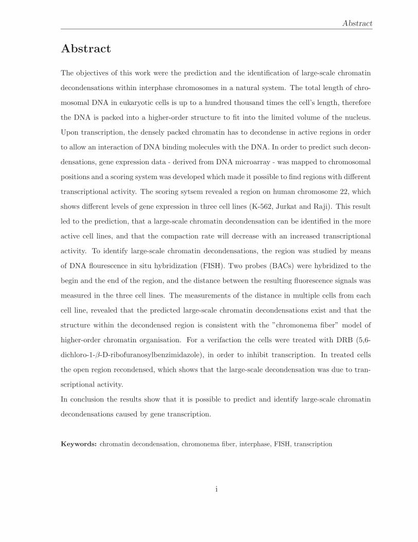
Abstract

The objectives of this work were the prediction and the identification of large-scale chromatin

decondensations within interphase chromosomes in a natural system. The total length of chro-

mosomal DNA in eukaryotic cells is up to a hundred thousand times the cell’s length, therefore

the DNA is packed into a higher-order structure to fit into the limited volume of the nucleus.

Upon transcription, the densely packed chromatin has to decondense in active regions in order

to allow an interaction of DNA binding molecules with the DNA. In order to predict such decon-

densations, gene expression data - derived from DNA microarray - was mapped to chromosomal

positions and a scoring system was developed which made it possible to find regions with different

transcriptional activity. The scoring sytsem revealed a region on human chromosome 22, which

shows different levels of gene expression in three cell lines (K-562, Jurkat and Raji). This result

led to the prediction, that a large-scale chromatin decondensation can be identified in the more

active cell lines, and that the compaction rate will decrease with an increased transcriptional

activity. To identify large-scale chromatin decondensations, the region was studied by means

of DNA flourescence in situ hybridization (FISH). Two probes (BACs) were hybridized to the

begin and the end of the region, and the distance between the resulting fluorescence signals was

measured in the three cell lines. The measurements of the distance in multiple cells from each

cell line, revealed that the predicted large-scale chromatin decondensations exist and that the

structure within the decondensed region is consistent with the ”chromonema fiber” model of

higher-order chromatin organisation. For a verifaction the cells were treated with DRB (5,6-

dichloro-1-β-D-ribofuranosylbenzimidazole), in order to inhibit transcription. In treated cells

the open region recondensed, which shows that the large-scale decondensation was due to tran-

scriptional activity.

In conclusion the results show that it is possible to predict and identify large-scale chromatin

decondensations caused by gene transcription.

Keywords: chromatin decondensation, chromonema fiber, interphase, FISH, transcription

i

Abstract

Kurzfassung

Ziel dieser Arbeit war es, ”umfangreiche Chromatin Dekondensationen” vorherzusagen und diese

dann zu identifizieren. Die Gesamtlange der chromosomalen DNA in eukaryotischen Zellen

betragt ein hunderttausendfaches der Lange einer Zelle. Um Platz im begrenzten Volumen eines

Zellkerns zu finden, ist die DNA als Struktur hoherer Ordnung verpackt. Wahrend der Gentran-

skription in der Interphase muss das dicht gepackte Chromatin in aktiven Bereichen eine dekon-

densierte Konformation annehmen, damit eine Interaktion von DNA-bindenden Molekulen mit

der DNA moglich wird. Um solche Dekondensationen vorhersagen zu konnen, wurden Genex-

pressionsdaten von DNA-Microarrays auf die chromosomale Position eines jeweiligen Gens abge-

bildet und ein Bewertungssystem entwickelt, das es ermoglichte Bereiche mit unterschiedlicher

Genexpression ausfindig zu machen. Mit Hilfe des Bewertungssystems wurde ein Bereich am

menschlichen Chromosom 22 gefunden, der in drei Zelllinien (K-562, Jurkat und Raji) eine un-

terschiedliche transkriptionelle Ativitat aufweist. Die Annahme war, dass man in den aktiveren

Zelllinien umfangreiche Chromatin Dekondensationen, in diesem Bereich beobachten konne, und

dass die Packungsdichte bei einer erhohten Genexpression abnimmt. Um solche umfangreiche

Chromatin Dekondensationen identifizieren zu konnen, wurde der Bereich mit Hilfe der DNA

FISH Technik untersucht. Zwei Sonden (BACs) wurden an den Anfang und das Ende des

Bereichs hybridisiert, worauf dann in den drei Zelllinen der Abstand zwischen den beiden re-

sultierenden Fluoreszenzsignalen gemessen wurde. Die Messungen des Abstandes in mehreren

Zellen jeder Zelllinie ergaben, dass die vorhergesagten Dekondensationen tatsachlich existieren,

und dass die Struktur des dekondensierten Bereichs dem ”Chromonema Fiber Model” fur die

Chromatin Organisation hoherer Ordnung entspricht. Als Kontrolle wurden die Zellen mit DRB

(5,6-Dichloro-1-β-D-Ribofuranosylbenzimidazol) behandelt, um die Transkription zu inhibieren.

Der Bereich lag nach der Inhibition wieder dicht gepackt vor, was beweist, dass die Dekonden-

sation durch transkriptionelle Aktivitat hervorgerufen wurde. Es ist also moglich, Chromatin

Dekondensationen vorherzusagen und zu identifizieren.

Schlusselworter: Chromatin Dekondensation, Chromonema Fiber, Interphase, FISH, Transkription

ii

Contents

Glossary ix

1 Introduction 1

1.1 DNA and its organization . . . . . . . . . . . . . . . . . . . . . . . . . . . 1

1.1.1 Basic DNA packing . . . . . . . . . . . . . . . . . . . . . . . . . . . 1

1.1.1.1 Beads on a String . . . . . . . . . . . . . . . . . . . . . . 2

1.1.1.2 The 30 nm fiber . . . . . . . . . . . . . . . . . . . . . . . 2

1.1.2 Higher order DNA packing . . . . . . . . . . . . . . . . . . . . . . . 4

1.1.2.1 Loops on a protein scaffold . . . . . . . . . . . . . . . . . 4

1.1.2.2 Chromonema fiber model . . . . . . . . . . . . . . . . . . 5

1.2 Transcription and chromatin . . . . . . . . . . . . . . . . . . . . . . . . . . 6

2 Objectives 8

2.1 Bioinformatics . . . . . . . . . . . . . . . . . . . . . . . . . . . . . . . . . . 8

2.2 Microscopy: FISH . . . . . . . . . . . . . . . . . . . . . . . . . . . . . . . . 9

3 Methods 10

3.1 Bioinformatics . . . . . . . . . . . . . . . . . . . . . . . . . . . . . . . . . 10

3.1.1 Perl . . . . . . . . . . . . . . . . . . . . . . . . . . . . . . . . . . . 11

3.1.1.1 The DBI module . . . . . . . . . . . . . . . . . . . . . . . 11

3.1.1.2 The GD module . . . . . . . . . . . . . . . . . . . . . . . 12

3.1.1.3 The Chart::Plot module . . . . . . . . . . . . . . . . . . . 12

iii

CONTENTS CONTENTS

3.1.1.4 The GFF module . . . . . . . . . . . . . . . . . . . . . . . 13

3.1.2 The General Feature Format - GFF . . . . . . . . . . . . . . . . . . 13

3.1.3 MySQL . . . . . . . . . . . . . . . . . . . . . . . . . . . . . . . . . 14

3.1.4 BLAST . . . . . . . . . . . . . . . . . . . . . . . . . . . . . . . . . 14

3.1.5 Microarray data . . . . . . . . . . . . . . . . . . . . . . . . . . . . . 14

3.1.5.1 Gene expression data extraction . . . . . . . . . . . . . . . 16

3.1.5.2 Error weighted exon expression . . . . . . . . . . . . . . . 16

3.1.6 Sequence data . . . . . . . . . . . . . . . . . . . . . . . . . . . . . . 17

3.1.6.1 Exon extraction . . . . . . . . . . . . . . . . . . . . . . . . 17

3.1.6.2 Gene extraction . . . . . . . . . . . . . . . . . . . . . . . . 18

3.1.7 The database . . . . . . . . . . . . . . . . . . . . . . . . . . . . . . 19

3.1.7.1 Sequence data . . . . . . . . . . . . . . . . . . . . . . . . 19

3.1.7.2 Gene expression data . . . . . . . . . . . . . . . . . . . . . 20

3.1.8 The scoring system . . . . . . . . . . . . . . . . . . . . . . . . . . . 21

3.1.8.1 The algorithm . . . . . . . . . . . . . . . . . . . . . . . . 22

3.1.9 Visualization of exon expression . . . . . . . . . . . . . . . . . . . . 23

3.2 Microscopy: FISH . . . . . . . . . . . . . . . . . . . . . . . . . . . . . . . . 24

3.2.1 The probe . . . . . . . . . . . . . . . . . . . . . . . . . . . . . . . . 26

3.2.1.1 BAC isolation . . . . . . . . . . . . . . . . . . . . . . . . . 27

3.2.1.2 BAC verification . . . . . . . . . . . . . . . . . . . . . . . 27

3.2.1.3 Biotin-Nick translation . . . . . . . . . . . . . . . . . . . . 28

3.2.1.4 Probe preparation for in situ hybridization . . . . . . . . . 29

3.2.2 The specimens . . . . . . . . . . . . . . . . . . . . . . . . . . . . . 30

3.2.2.1 Cell cultures . . . . . . . . . . . . . . . . . . . . . . . . . 30

3.2.2.2 Preparation of coverslips . . . . . . . . . . . . . . . . . . . 30

3.2.2.3 Cell fixation . . . . . . . . . . . . . . . . . . . . . . . . . . 31

3.2.2.4 Cell permeabilization . . . . . . . . . . . . . . . . . . . . . 31

3.2.2.5 RNase treatment . . . . . . . . . . . . . . . . . . . . . . . 31

3.2.2.6 DNA denaturation . . . . . . . . . . . . . . . . . . . . . . 32

iv

CONTENTS CONTENTS

3.2.3 Hybridization . . . . . . . . . . . . . . . . . . . . . . . . . . . . . . 32

3.2.4 Detection . . . . . . . . . . . . . . . . . . . . . . . . . . . . . . . . 33

3.2.5 Measurements . . . . . . . . . . . . . . . . . . . . . . . . . . . . . . 33

4 Results 35

4.1 Bioinformatics . . . . . . . . . . . . . . . . . . . . . . . . . . . . . . . . . . 35

4.1.1 Microarray data . . . . . . . . . . . . . . . . . . . . . . . . . . . . . 35

4.1.2 Region localization through BAC mapping . . . . . . . . . . . . . . 36

4.1.3 Scoring system . . . . . . . . . . . . . . . . . . . . . . . . . . . . . 37

4.1.4 Regions with potential chromatin decondensation . . . . . . . . . . 37

4.1.4.1 Expression profiles . . . . . . . . . . . . . . . . . . . . . . 39

4.1.5 Conclusion . . . . . . . . . . . . . . . . . . . . . . . . . . . . . . . . 40

4.2 Microscopy: FISH . . . . . . . . . . . . . . . . . . . . . . . . . . . . . . . . 40

4.2.1 The probes . . . . . . . . . . . . . . . . . . . . . . . . . . . . . . . 40

4.2.1.1 BAC isolation . . . . . . . . . . . . . . . . . . . . . . . . . 40

4.2.1.2 BAC verification . . . . . . . . . . . . . . . . . . . . . . . 41

4.2.2 Hybridization . . . . . . . . . . . . . . . . . . . . . . . . . . . . . . 42

4.2.2.1 K-562 and BAC 3 . . . . . . . . . . . . . . . . . . . . . . 42

4.2.2.2 K-562 and BAC 3 versus Raji and BAC 3 . . . . . . . . . 44

4.2.2.3 Amplifications in K-562 . . . . . . . . . . . . . . . . . . . 45

4.2.2.4 Raji and BAC 3 . . . . . . . . . . . . . . . . . . . . . . . 46

4.2.2.5 Jurkat and BAC 3 + BAC 22 versus Raji and BAC 3 +

BAC 22 . . . . . . . . . . . . . . . . . . . . . . . . . . . . 47

4.2.2.6 DRB treated Jurkat and BAC 3 + BAC 22 . . . . . . . . 49

4.2.3 Chromatin compaction rate . . . . . . . . . . . . . . . . . . . . . . 50

5 Discussion 51

References 54

Index 60

v

CONTENTS CONTENTS

A Protocols 62

A.1 DNA FISH . . . . . . . . . . . . . . . . . . . . . . . . . . . . . . . . . . . 62

A.1.1 Specimen preparation, hybridization and detection . . . . . . . . . 62

A.1.2 Probe preparation . . . . . . . . . . . . . . . . . . . . . . . . . . . 64

A.2 Glycerol cultures . . . . . . . . . . . . . . . . . . . . . . . . . . . . . . . . 65

A.3 Freezing cells for conservation . . . . . . . . . . . . . . . . . . . . . . . . . 65

B Gene-list 66

vi

List of Figures

1.1 beads-on-a-string . . . . . . . . . . . . . . . . . . . . . . . . . . . . . . . . 2

1.2 The 30 nm fiber . . . . . . . . . . . . . . . . . . . . . . . . . . . . . . . . . 3

1.3 Basic DNA packing . . . . . . . . . . . . . . . . . . . . . . . . . . . . . . . 3

1.4 DNA Loops on a protein scaffold . . . . . . . . . . . . . . . . . . . . . . . 5

1.5 Chromonema model . . . . . . . . . . . . . . . . . . . . . . . . . . . . . . . 6

3.1 DBI Application Architecture . . . . . . . . . . . . . . . . . . . . . . . . . 12

3.2 Data model . . . . . . . . . . . . . . . . . . . . . . . . . . . . . . . . . . . 21

3.3 FISH flowchart . . . . . . . . . . . . . . . . . . . . . . . . . . . . . . . . . 25

3.4 BAC vector . . . . . . . . . . . . . . . . . . . . . . . . . . . . . . . . . . . 26

3.5 Agarose gel: BAC isolation . . . . . . . . . . . . . . . . . . . . . . . . . . . 27

3.6 Agarose gel: nick tanslation . . . . . . . . . . . . . . . . . . . . . . . . . . 28

4.1 Transcription plots . . . . . . . . . . . . . . . . . . . . . . . . . . . . . . . 38

4.2 BAC mapping . . . . . . . . . . . . . . . . . . . . . . . . . . . . . . . . . . 41

4.3 Hybridization: K-562 / BAC 3 . . . . . . . . . . . . . . . . . . . . . . . . . 42

4.4 BAC size distribution: K-562 . . . . . . . . . . . . . . . . . . . . . . . . . 43

4.5 K-562 deconvolution . . . . . . . . . . . . . . . . . . . . . . . . . . . . . . 43

4.6 Hybridization: K-562 versus Raji . . . . . . . . . . . . . . . . . . . . . . . 44

4.7 BAC size distribution: K-562 / Raji . . . . . . . . . . . . . . . . . . . . . . 44

4.8 K-562 metaphase FISH . . . . . . . . . . . . . . . . . . . . . . . . . . . . . 45

4.9 Hybridization: Raji / BAC 3 . . . . . . . . . . . . . . . . . . . . . . . . . . 46

4.10 BAC size distribution: Raji / BAC 3 . . . . . . . . . . . . . . . . . . . . . 46

vii

LIST OF FIGURES LIST OF FIGURES

4.11 Hybridization: Jurkat versus Raji / 2 BACs . . . . . . . . . . . . . . . . . 47

4.12 BAC distance distribution: Jurkat versus Raji /2 BACs . . . . . . . . . . . 47

4.13 Hybridization: Jurkat / 2 BACs . . . . . . . . . . . . . . . . . . . . . . . . 49

4.14 BAC distance distribution: Jurkat versus Jurkat + DRB . . . . . . . . . . 49

viii

Glossary

acrocentric a chromosome with the centromere towards one end is acrocentric.

awk is a pattern scanning and processing language. It scans each input file for lines

that match any of a set of specified patterns.

API stands for ”Application Programming Interface” and provides a set of functions

and classes that can be used to develop an application.

BAC bacterial artificial chromosomes are vectors similar to standard E. coli plasmid

vectors except that they contain the origin and genes encoding the ORI-binding proteins

required for plasmid replication from a naturally occurring large E. coli plasmid called

the F-factor. Inserts can be up to 300 Kbp in size.

C is a programming language.

CCD a charge coupled device is a collection of tiny light-sensitive diodes, which convert

photons (light) into electrons (electrical charge). A CCD camera can be used to acquire

digital images.

cDNA complementary DNA is a form of DNA prepared in the laboratory using mes-

senger RNA (mRNA) as template, i.e. the reverse of the usual process of transcription in

cells; the synthesis is catalyzed by reverse transcriptase. cDNA thus has a base sequence

ix

Glossary

that is complementary to that of the mRNA template; unlike genomic DNA, it contains

no noncoding sequences (introns).

centromere constricted portion of a mitotic chromosome where sister chromatids are

attached. It is required for proper chromosome segregation during mitosis and meiosis.

chromatid one copy of a duplicated chromosome, formed during the S phase of the cell

cycle, that is still joined at the centromere to the other copy; also called sister chromatid.

During mitosis, the two chromatids separate, each becoming a chromosome of one of the

two daughter cells.

chromatin complex of DNA, histones, and nonhistone proteins from which eukaryotic

chromosomes are formed. Condensation of chromatin during mitosis yields the visible

metaphase chromosomes.

CPAN stands for Comprehensive Perl Archive Network; it’s a globally replicated trove

of Perl materials.

cy3 fluorescent dye, green; used for labeling RNA in microarray experiments.

cy5 fluorescent dye, red; used for labeling RNA in microarray experiments.

deconvolution is a process of relocating signal scatter and out-of-focus information

present in digital images. The image seen in the microscope also contains blur from out-

of-focus light and light scatter in the specimen. This blur results from the convolution

of the specimen with the microscope’s Point Spread Function (PSF). By reversing this

blurring through the constrained-iterative deconvolution process, the image is clarified

and its data is quantitatively restored.

DNA deoxyribonucleic acid is a long linear polymer, composed of four kinds of deoxyri-

bose nucleotides, that is the carrier of genetic information.

x

Glossary

DNase an enzyme that catalyzes the cleavage of DNA. DNAase I is a digestive enzyme,

that degrades DNA into shorter nucleotide fragments.

euchromatin less condensed portions of chromatin, including most transcribed regions,

present in interphase chromosomes. See also heterochromatin.

exon segments of a eukaryotic gene (or of its primary transcript) that reaches the cy-

toplasm as part of a mature mRNA, rRNA, or tRNA molecule. See also intron.

grep program that searches the named input files (or standard input if no files are

named) for lines containing a match to the given pattern.

heterochromatin regions of chromatin that remain highly condensed and transcrip-

tionally inactive during interphase.

insert piece of DNA that is cloned into a vector.

intron part of a primary transcript (or the DNA encoding it) that is removed by splicing

during RNA processing and is not included in the mature, functional mRNA, rRNA, or

tRNA;

JPEG compressed graphics format.

metaphase mitotic stage at which chromosomes are fully condensed and attached to

the mitotic spindle at its equator but have not yet started to segregate toward the opposite

spindle poles.

mitosis in eukaryotic cells, the process whereby the nucleus is divided to produce two

genetically equivalent daughter nuclei with the diploid number of chromosomes.

xi

Glossary

NCBI National Center for Biotechnology Information. NCBI creates public databases,

conducts research in computational biology, develops software tools for analyzing genome

data, and disseminates biomedical information.

ONC Over Night Culture. Cell grown over night.

oncogene a gene whose product is involved either in transforming cells in culture or in

inducing cancer in animals. Most oncogenes are mutant forms of normal genes (proto-

oncogenes) involved in the control of cell growth or division.

PBS Phosphate-Buffered Saline; 0.02 M sodium phosphate buffer with 0.15 M sodium

chloride

plasmid small, circular extrachromosomal DNA molecule capable of autonomous repli-

cation in a cell. Commonly used as a cloning vector.

PNG Portable Network Graphics. Graphics format.

RNA ribonucleic acid is a linear, single-stranded polymer, composed of ribose nu-

cleotides, that is synthesized by transcription of DNA or by copying of RNA. The three

types of cellular RNA - mRNA, rRNA, and tRNA - play different roles in protein synthesis.

sed is a stream editor. A stream editor is used to perform basic text transformations

on an input stream.

sh is a command programming language that executes commands read from a terminal

or a file.

sort is a program which sorts lines of all the named files together and writes the result

on the standard output.

xii

Glossary

SSC Saline-Sodium Citrate buffer for ISH procedures.

STS stands for ”sequence tagged sites”; short sequences that are operationally unique

in the genome, used to generate mapping reagents.

vector in cell biology, an agent that can carry DNA into a cell or organism.

XML Extensible Markup Language (XML) is a simple, very flexible text format. Orig-

inally designed to meet the challenges of large-scale electronic publishing, XML is also

playing an increasingly important role in the exchange of a wide variety of data on the

Web and elsewhere.

zip archive zip files are ”archives” used for distributing and storing files. Zip files

contain one or more files. Usually the files ”archived” in a Zip are compressed to save

space. Zip files make it easy to group files and make transporting and copying these files

faster.

xiii

Chapter 1

Introduction

1.1 DNA and its organization

The genetic information of living organisms is carried by DNA, which can be seen as a

storehouse, or cellular library, that contains all the information required for building cells

and tissues. DNA is an enormously long polymeric molecule. Basically it consits of a

sequence of four different subunits, the so called nucleotides. Cellular DNA molecules

can be as long as several hundred million nucleotides, arranged in an irregular but non-

random sequence. Every million nucleotides take up a linear distance of 3.4 x 105 nm

(0.034 cm). The human genome consists of about 6 x 109 nucleotide pairs, organized in 2

x 23 different DNA molecules, the chromosomes - each containing 50 x 106 to 250 x 106

nucleotide pairs. DNA molecules of this size have a linear length of 1.7 to 8.5 cm.

1.1.1 Basic DNA packing

Because the total length of chromosomal DNA in cells is up to a hundred thousand times

the cell’s length, the packing of DNA into a compact structure is crucial. The DNA must

fit in a nucleus of only a few micrometers in diameter.

1

Introduction 1.1 DNA and its organization

1.1.1.1 Beads on a String

DNA from eukaryotic nuclei is associated with an

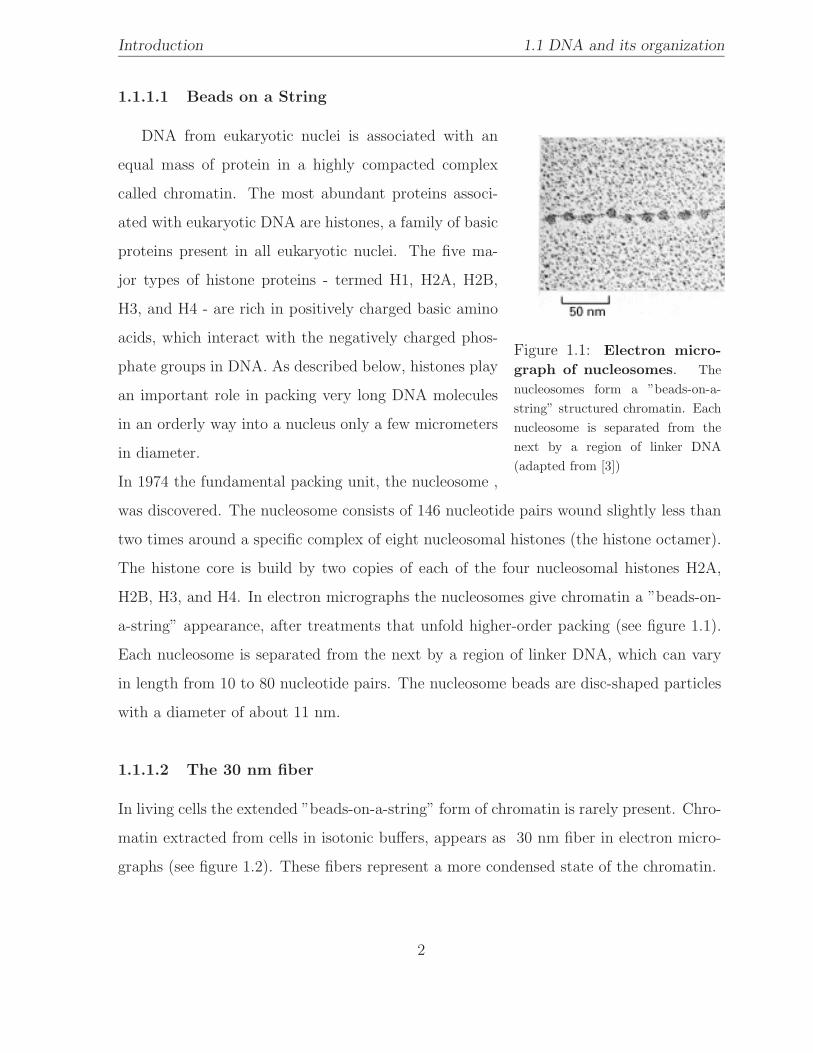
Figure 1.1: Electron micro-graph of nucleosomes. Thenucleosomes form a ”beads-on-a-string” structured chromatin. Eachnucleosome is separated from thenext by a region of linker DNA(adapted from [3])

equal mass of protein in a highly compacted complex

called chromatin. The most abundant proteins associ-

ated with eukaryotic DNA are histones, a family of basic

proteins present in all eukaryotic nuclei. The five ma-

jor types of histone proteins - termed H1, H2A, H2B,

H3, and H4 - are rich in positively charged basic amino

acids, which interact with the negatively charged phos-

phate groups in DNA. As described below, histones play

an important role in packing very long DNA molecules

in an orderly way into a nucleus only a few micrometers

in diameter.

In 1974 the fundamental packing unit, the nucleosome ,

was discovered. The nucleosome consists of 146 nucleotide pairs wound slightly less than

two times around a specific complex of eight nucleosomal histones (the histone octamer).

The histone core is build by two copies of each of the four nucleosomal histones H2A,

H2B, H3, and H4. In electron micrographs the nucleosomes give chromatin a ”beads-on-

a-string” appearance, after treatments that unfold higher-order packing (see figure 1.1).

Each nucleosome is separated from the next by a region of linker DNA, which can vary

in length from 10 to 80 nucleotide pairs. The nucleosome beads are disc-shaped particles

with a diameter of about 11 nm.

1.1.1.2 The 30 nm fiber

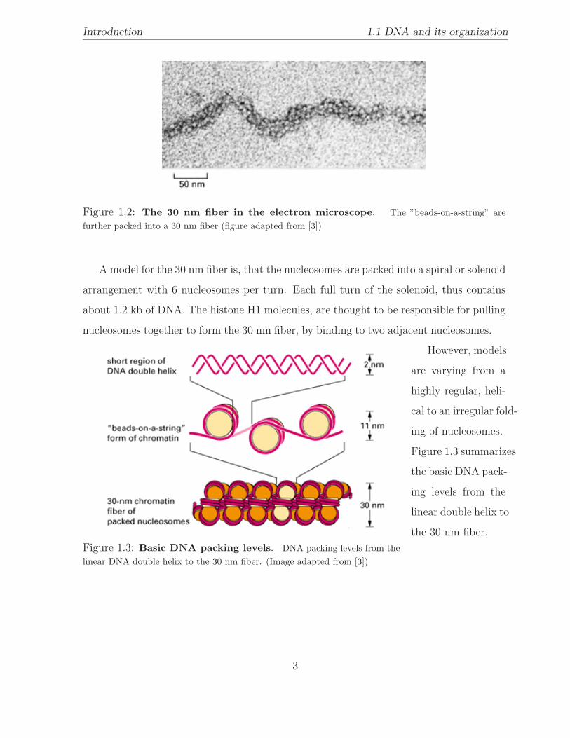
In living cells the extended ”beads-on-a-string” form of chromatin is rarely present. Chro-

matin extracted from cells in isotonic buffers, appears as 30 nm fiber in electron micro-

graphs (see figure 1.2). These fibers represent a more condensed state of the chromatin.

2

Introduction 1.1 DNA and its organization

Figure 1.2: The 30 nm fiber in the electron microscope. The ”beads-on-a-string” arefurther packed into a 30 nm fiber (figure adapted from [3])

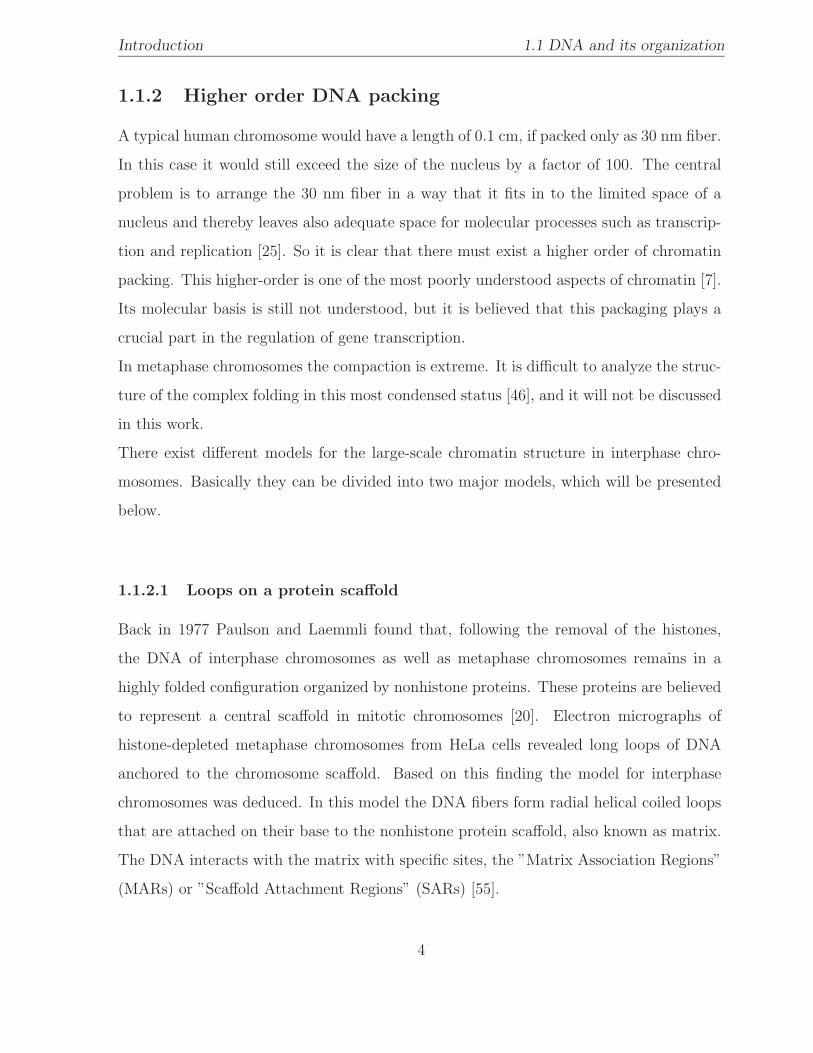
A model for the 30 nm fiber is, that the nucleosomes are packed into a spiral or solenoid

arrangement with 6 nucleosomes per turn. Each full turn of the solenoid, thus contains

about 1.2 kb of DNA. The histone H1 molecules, are thought to be responsible for pulling

nucleosomes together to form the 30 nm fiber, by binding to two adjacent nucleosomes.

However, models

Figure 1.3: Basic DNA packing levels. DNA packing levels from thelinear DNA double helix to the 30 nm fiber. (Image adapted from [3])

are varying from a

highly regular, heli-

cal to an irregular fold-

ing of nucleosomes.

Figure 1.3 summarizes

the basic DNA pack-

ing levels from the

linear double helix to

the 30 nm fiber.

3

Introduction 1.1 DNA and its organization

1.1.2 Higher order DNA packing

A typical human chromosome would have a length of 0.1 cm, if packed only as 30 nm fiber.

In this case it would still exceed the size of the nucleus by a factor of 100. The central

problem is to arrange the 30 nm fiber in a way that it fits in to the limited space of a

nucleus and thereby leaves also adequate space for molecular processes such as transcrip-

tion and replication [25]. So it is clear that there must exist a higher order of chromatin

packing. This higher-order is one of the most poorly understood aspects of chromatin [7].

Its molecular basis is still not understood, but it is believed that this packaging plays a

crucial part in the regulation of gene transcription.

In metaphase chromosomes the compaction is extreme. It is difficult to analyze the struc-

ture of the complex folding in this most condensed status [46], and it will not be discussed

in this work.

There exist different models for the large-scale chromatin structure in interphase chro-

mosomes. Basically they can be divided into two major models, which will be presented

below.

1.1.2.1 Loops on a protein scaffold

Back in 1977 Paulson and Laemmli found that, following the removal of the histones,

the DNA of interphase chromosomes as well as metaphase chromosomes remains in a

highly folded configuration organized by nonhistone proteins. These proteins are believed

to represent a central scaffold in mitotic chromosomes [20]. Electron micrographs of

histone-depleted metaphase chromosomes from HeLa cells revealed long loops of DNA

anchored to the chromosome scaffold. Based on this finding the model for interphase

chromosomes was deduced. In this model the DNA fibers form radial helical coiled loops

that are attached on their base to the nonhistone protein scaffold, also known as matrix.

The DNA interacts with the matrix with specific sites, the ”Matrix Association Regions”

(MARs) or ”Scaffold Attachment Regions” (SARs) [55].

4

Introduction 1.1 DNA and its organization

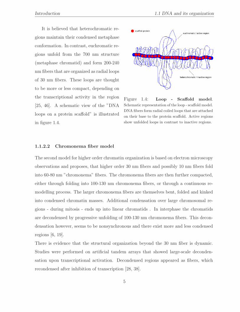
It is believed that heterochromatic re-

Figure 1.4: Loop - Scaffold model.Schematic representation of the loop - scaffold model.DNA fibers form radial coiled loops that are attachedon their base to the protein scaffold. Active regionsshow unfolded loops in contrast to inactive regions.

gions maintain their condensed metaphase

conformation. In contrast, euchromatic re-

gions unfold from the 700 nm structure

(metaphase chromatid) and form 200-240

nm fibers that are organized as radial loops

of 30 nm fibers. These loops are thought

to be more or less compact, depending on

the transcriptional activity in the region

[25, 46]. A schematic view of the ”DNA

loops on a protein scaffold” is illustrated

in figure 1.4.

1.1.2.2 Chromonema fiber model

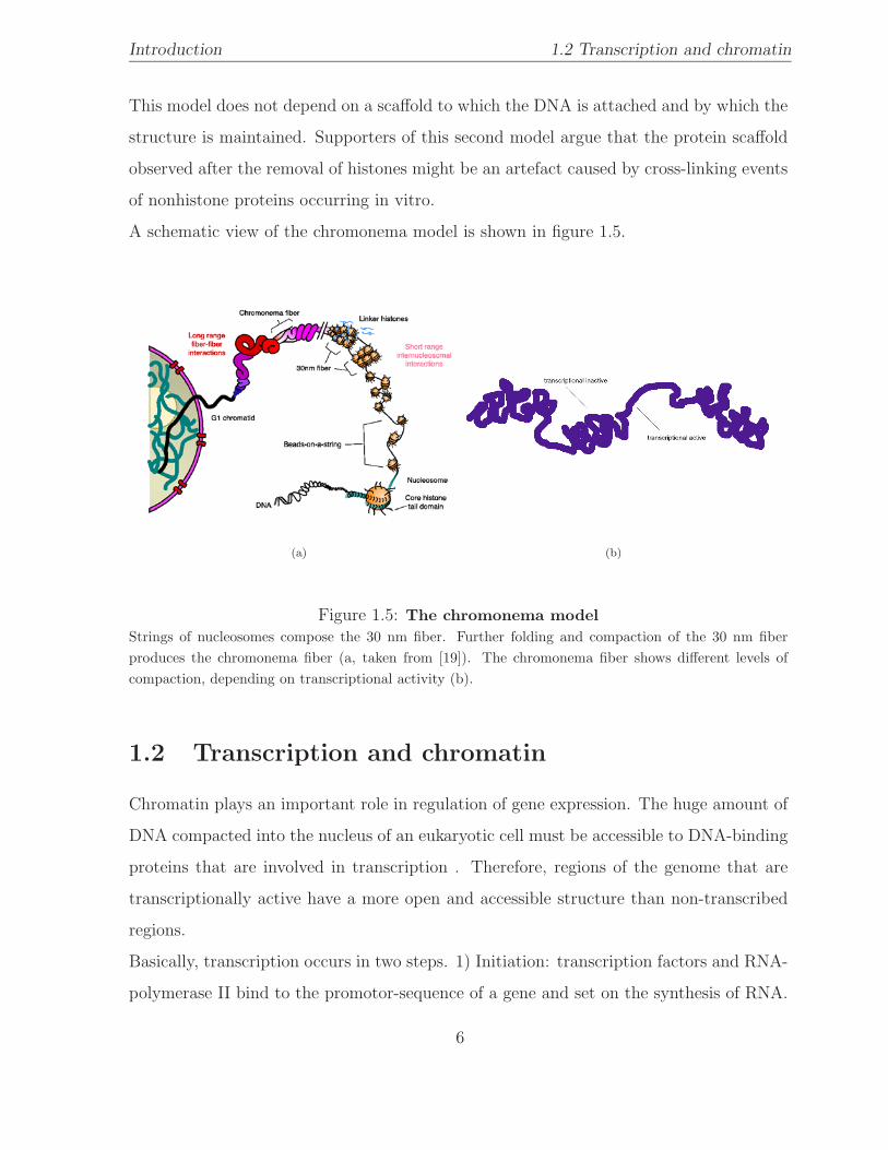
The second model for higher order chromatin organization is based on electron microscopy

observations and proposes, that higher order 30 nm fibers and possibly 10 nm fibers fold

into 60-80 nm ”chromonema” fibers. The chromonema fibers are then further compacted,

either through folding into 100-130 nm chromonema fibers, or through a continuous re-

modelling process. The larger chromonema fibers are themselves bent, folded and kinked

into condensed chromatin masses. Additional condensation over large chromosomal re-

gions - during mitosis - ends up into linear chromatids . In interphase the chromatids

are decondensed by progressive unfolding of 100-130 nm chromonema fibers. This decon-

densation however, seems to be nonsynchronous and there exist more and less condensed

regions [6, 19].

There is evidence that the structural organization beyond the 30 nm fiber is dynamic.

Studies were performed on artificial tandem arrays that showed large-scale deconden-

sation upon transcriptional activation. Decondensed regions appeared as fibers, which

recondensed after inhibition of transcription [28, 38].

5

Introduction 1.2 Transcription and chromatin

This model does not depend on a scaffold to which the DNA is attached and by which the

structure is maintained. Supporters of this second model argue that the protein scaffold

observed after the removal of histones might be an artefact caused by cross-linking events

of nonhistone proteins occurring in vitro.

A schematic view of the chromonema model is shown in figure 1.5.

(a) (b)

Figure 1.5: The chromonema modelStrings of nucleosomes compose the 30 nm fiber. Further folding and compaction of the 30 nm fiberproduces the chromonema fiber (a, taken from [19]). The chromonema fiber shows different levels ofcompaction, depending on transcriptional activity (b).

1.2 Transcription and chromatin

Chromatin plays an important role in regulation of gene expression. The huge amount of

DNA compacted into the nucleus of an eukaryotic cell must be accessible to DNA-binding

proteins that are involved in transcription . Therefore, regions of the genome that are

transcriptionally active have a more open and accessible structure than non-transcribed

regions.

Basically, transcription occurs in two steps. 1) Initiation: transcription factors and RNA-

polymerase II bind to the promotor-sequence of a gene and set on the synthesis of RNA.

6

Introduction 1.2 Transcription and chromatin

2) Elongation: the polymerase moves along the DNA and synthesizes an RNA transcript.

In the past a lot of studies focused on the accessibility of DNA on transcription initiation

sites. They revealed local changes in nucleosome structure and histone modifications. For

example, histone H1, is depleted at active sites, tails of other histones become actetylated

[30]. But not only local changes of chromatin structure occur in transcriptionally active

regions. Evidence for this provides the increased nuclease sensitivity of transcribed re-

gions, and microscopic observations of active regions [38, 37, 28], which show large-scale

unfoldings of actively transcribed chromatin, rather then localized decondensation.

7

Chapter 2

Objectives

The goal of this project was to predict and identify large scale chromatin decondensations

within interphase chromosomes in a natural system.

In previous work, several groups could already show large scale chromatin decondensation

[28, 37, 38]. However, these studies were based on artificial tandem arrays integrated into

chromosomes rather than on natural sequences. Thus, these systems could only serve as

models for large scale chromatin organization and suggest how it might look in a natural

system.

In order to find out what the large scale chromatin structure looks like in a natural system

an unbiased approach was considered. This approach was divided into two major tasks,

which will be described in this section.

2.1 Bioinformatics

It was described before [13] that genes with similar functions tend to occur in adjacent

positions along a chromosome and are co-expressed. Such groups of correlated adjacent

genes appear throughout the genome and show a statistical significant occurrence. More

recent studies [9, 33] confirm these findings. These results suggest that these gene clusters

may correspond to regions of active chromatin, because opening chromatin for one gene

can result in the opening of neighbouring chromatin [18, 36], transcriptional machinery

8

Objectives 2.2 Microscopy: FISH

may access two co-expressed genes more efficiently if they are neighbours than if they are

apart.

These results show that a large scale chromatin decondensation could be found in regions

of co-regulated and active genes. To identify such regions an analysis of microarray

data using bioinformatic methods was considered. The result of the analysis should give

predictions of different levels of chromatin compaction on a specific chromosomal region,

either in different cell lines or in one cell line under different conditions.

2.2 Microscopy: FISH

The second part of this work was the identification of large scale chromatin decon-

densations using the DNA FISH technique. Based on the results from the microarray

analysis, a chromosomal region which is predicted to show changes in chromatin struc-

ture/compaction caused by transcription, should be examined by fluorescence microscopy.

Fluorescence in situ hybridization makes it possible to visualize single sequences within

decondensed interphase chromosomes [21]. Thus it should be possible to use this tech-

nique to look at the predicted sequences/regions, and determine if there are differences

in chromatin structure between two cell lines.

9

Chapter 3

Methods

3.1 Bioinformatics

To discover regions on a chromosome that show differences in their gene expression level

in a large scale format, an analysis of public available microarray data was considered.

cDNA microarrays are capable of profiling gene expression patterns of tens of thousands

of genes in a single experiment [14]. Thus, it is also possible to monitor the expression

of all genes, even all exons along a whole chromosome with this technology. Data sets

originating from such experiments are usually hard to handle by conventional methods

(data reading, spread sheets), for they can contain the information of tens of thousand of

probes across multiple experiments or time points.

Bioinformatic methods can help to deal with the huge amount of data produced by DNA

microarray experiments.

In this work a relational database management system (RDBMS) MySQL [48] and the

programming language Perl [47] was used in order to handle, retrieve, store and manage

data derived from microarray experiments.

As further analysis tool, BLAST came in use to map and verify DNA sequences.

10

Methods 3.1 Bioinformatics

3.1.1 Perl

Perl is a programming language optimized for scanning arbitrary text files, extracting

information from those text files, and printing reports based on that information. The

language is intended to be practical (easy to use, efficient, complete). Perl can use sophis-

ticated pattern matching techniques to scan large amounts of data quickly. It combines

some of the best features of C, sed, awk, and sh, so people familiar with those languages

have little difficulty with it. Expression syntax corresponds closely to C expression syn-

tax. Unlike most Unix utilities, Perl does not arbitrarily limit the size of data [47]. Other

benefits of Perl are modularity and reusability of already existing code using modules.

Extension modules are written in C (or a mix of Perl and C). They are usually dynami-

cally loaded into Perl if and when they are needed, but may also be linked in statically.

C extension modules like DBI (3.1.1.1), GD (3.1.1.2) or Chart::Plot (3.1.1.3) which were

used for this work, can be found on CPAN [2].

Because of the features of Perl, it was chosen in this work as programming language to

develop programs, which deal with the large amount of data coming from the microarray

experiments.

3.1.1.1 The DBI module

The DBI (Database Interface) is a database access module for the Perl programming

language. It defines a set of methods, variables, and conventions that provide a consistent

database interface, independent of the actual database being used. It is a layer of ”glue”

between an application and one or more database driver modules. It is the driver modules

which do most of the real work. The DBI provides a standard interface and framework

for the drivers to operate within [8].

Architecture of a DBI Application: The API , or Application Programming Inter-

face, defines the call interface and variables for Perl scripts to use. The API is implemented

by the Perl DBI extension. The DBI ”dispatches” the method calls to the appropriate

driver for actual execution. The DBI is also responsible for the dynamic loading of drivers,

11

Methods 3.1 Bioinformatics

error checking and handling, providing default implementations for methods, and many

other non-database specific duties. Each driver contains implementations of the DBI

methods using the private interface functions of the corresponding database engine. Only

authors of sophisticated/multi-database applications or generic library functions need be

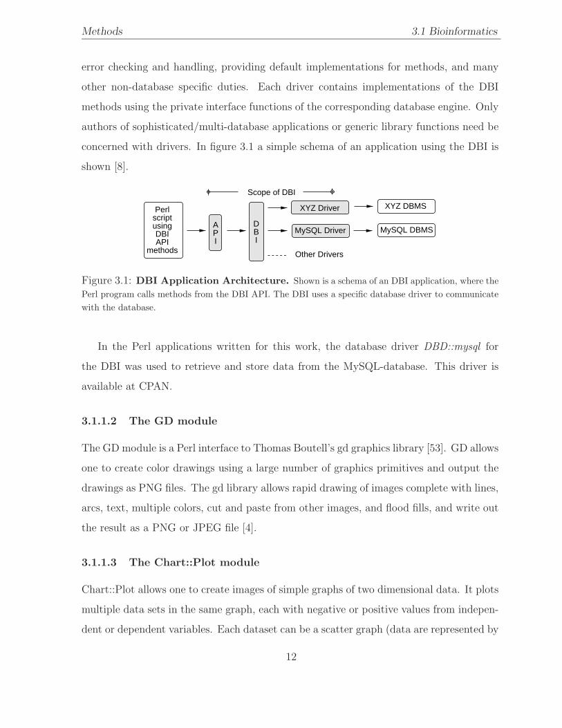
concerned with drivers. In figure 3.1 a simple schema of an application using the DBI is

shown [8].

PerlscriptusingDBIAPI

methods

API

DBI

XYZ Driver

MySQL Driver

Other Drivers

XYZ DBMS

MySQL DBMS

Scope of DBI

Figure 3.1: DBI Application Architecture. Shown is a schema of an DBI application, where thePerl program calls methods from the DBI API. The DBI uses a specific database driver to communicatewith the database.

In the Perl applications written for this work, the database driver DBD::mysql for

the DBI was used to retrieve and store data from the MySQL-database. This driver is

available at CPAN.

3.1.1.2 The GD module

The GD module is a Perl interface to Thomas Boutell’s gd graphics library [53]. GD allows

one to create color drawings using a large number of graphics primitives and output the

drawings as PNG files. The gd library allows rapid drawing of images complete with lines,

arcs, text, multiple colors, cut and paste from other images, and flood fills, and write out

the result as a PNG or JPEG file [4].

3.1.1.3 The Chart::Plot module

Chart::Plot allows one to create images of simple graphs of two dimensional data. It plots

multiple data sets in the same graph, each with negative or positive values from indepen-

dent or dependent variables. Each dataset can be a scatter graph (data are represented by

12

Methods 3.1 Bioinformatics

graph points only) or lines connecting successive data points, or both. Colors and dashed

lines are supported. Axes are scaled and positioned automatically, ticks are drawn and

labeled on each axis [49]. This Perl module requires the GD module.

3.1.1.4 The GFF module

GFF is a Perl Object base class/module for the General Feature Format (GFF) 3.1.2.

It allows one to read, parse and handle data in the GFF format. It provides also the

possibility to write GFF files, merging different GFF data sets and sorting GFF features

[54].

3.1.2 The General Feature Format - GFF

GFF is a format for describing genes and other features, like exons, introns, polyA-sites

etc. associated with DNA, RNA and protein sequences.

The GFF format is intended to be easy to parse and process by a variety of programs

in different languages. For example, Unix tools like grep, sort and simple Perl and awk

scripts can easily extract information out of a GFF file. For these reasons it has a record-

based structure, where each feature is described on a single line, and the line order is

not relevant [51]. A GFF record is an extension of a basic (name, start, end) tuple (or

”NSE”) that can be used to identify a substring of a biological sequence. For example,

the NSE (ChromosomeI, 2000, 3000) specifies the third kilobase of the sequence named

”ChromosomeI”.

The most common operations that one typically wants to perform on sets of NSEs and

NSE-pairs include intersection, exclusion, union, filtration, sorting, transformation (to a

new co-ordinate system) and dereferencing (access to the described sequence). With a

suitably flexible definition of NSE ”similarity”, these operations form a basis for more

sophisticated algorithms like clustering and joining-together by dynamic programming.

13

Methods 3.1 Bioinformatics

3.1.3 MySQL

MySQL , a popular Open Source SQL database, is developed, distributed and supported

by MySQL AB. A database is a structured collection of data. It may contain any infor-

mation from a simple shopping list to a picture gallery or vast amounts of information

like biological data. To add, access, and process data stored in a computer database, a

database management system (DBMS ) such as the MySQL Server is needed.

MySQL is a relational database management system (RDBMS ). A relational database

stores data in separate tables rather than putting all the data in one big storeroom. This

adds speed and flexibility. The tables are linked by defined relations making it possible

to combine data from several tables on request. The SQL part of ”MySQL” stands for

”Structured Query Language”, the most common standardized language used to access

databases [48].

3.1.4 BLAST

BLAST (Basic Local Alignment Search Tool) is a tool for sequence similarity searches.

It can be used to compare both, protein or DNA sequences. BLAST uses a heuristic

algorithm to seek local alignments and is therefore able to detect similarities among

sequences, even if they share only isolated regions of similarity [5].

The BLAST program set was downloaded from NCBI (ftp://ftp.ncbi.nih.gov/blast/). For

the sequence mapping (see 3.1.8) and verification (see 3.2.1.2) in this work the megablast

tool, which makes part of the BLAST tool set, was utilized, because it is optimized for

aligning sequences that differ slightly. It is also able to efficiently handle much lager DNA

sequences than the traditional blastn program.

3.1.5 Microarray data

For an accurate prediction of transcriptional mediated chromatin decondensation it was

necessary to have gene expression data that covers a whole chromosome. It was also im-

portant, that the genes (probes) on the microarray were annotated and their chromosomal

14

Methods 3.1 Bioinformatics

position was known. Therefore, public available gene expression data from microarray ex-

periments, that meets these requirements, were searched.

The search led to several sources. One of them was the whole-genome mRNA expression

data generated for the mitotic cell cycle of S. cerevisiae [11]. The disadvantage of the

yeast in terms of identifying large scale chromatin structures by fluorescence microscopy,

is that the yeast chromosomes are relatively small (largest 2.2 Mbp). In previous stud-

ies [28] large scale decondensation of the MMTV array (mouse mammary tumor virus),

where the most decondensed arrays had a 50-fold chromatin compaction, could be shown.

This construct has a length of ≥ 2 Mbp, which is about the size of the largest yeast

chromosome, and is build homogeneously by ≥ 200 repeats of a 9 Kbp sequence [27].

The detection limit of the light microscope is about 0.4 µm, that means that a detectable

decondensed structure would already require a size of ∼60 Kbp and would produce a dot

shaped image. It is unlikely that a natural chromosome is as homogeneous in its sequence

as the MMTV, thus one could expect a higher compaction rate in decondensed regions.

Therefore it may require a size of ∼0.5-1 Mbp to see large-scale chromatin decondensa-

tions on a natural chromosome and to be able to study its structure. It is unlikely that

a good part or even a whole chromosome is transcriptional active in yeast at the same

time. To be sure that the structure of an active gene cluster could also be identified and

studied by DNA FISH, the decision was made to use data of an organism with larger

chromosomes.

A data set which satisfied all the requirements (annotation, probes with known chro-

mosomal positions, whole coverage of a chromosome, large chromosomes) came from an

experimental annotation of the human chromosome 22q using microarrays [34]. In this

work the authors describe a high-throughput, microarray-based experimental method to

validate predicted exons , group the exons into genes by coregulated expression and define

full-length mRNA transcripts. Chromosome 22 was the first human chromosome to be

completely sequenced and annotated [15]. Shoemaker et. al. designed a single ink-jet

microarray to validate the 8,183 exons annotated [15] on chromosome 22q under different

experimental conditions. The mRNAs from human cell lines and tissues were fluorescently

15

Methods 3.1 Bioinformatics

labeled with two dyes (cy3 and cy5) and hybridized in pairs to 69 individual chromosome

22 exon arrays. The probes on the exon arrays based on 6,650 Genscan-predicted exon

sequences, and 3,381 validated exon sequences [34]. From this set of 10,031 exons 1,848

were identical and thus removed form the pool. For each of the resulting 8,183 exon se-

quences two 60-mers were selected as probes on the microarray. For exon sequences with

60 or less nucleotides, a single probe consisting of the entire sequence was used. This led

to an array with 15,511 60-mers, which covered the whole q-arm of chromosome 22.

3.1.5.1 Gene expression data extraction

The results of the microarray experiment from Rosetta Inpharmatics were downloaded

from the company’s website [42] as a 220Mb zip archive. It contained a directory for each

of the 69 experiments. These directories contained data files for the experiment and the

corresponding reversed flour experiments. The expression data in these files were stored

in the GEMLTM [43] format.

Gene Expression Markup Language (GEML) is an XML file specification for converting

DNA microarray and gene expression data into a common format. To extract the needed

data from these files a Perl program, which parsed the formatted text and produced tab

separated lists as output, was written. The extracted fields were the following: probename,

raw and normalized value for the cy3 and cy5 channel, log10cy5cy3

, error of log10cy5cy3

(=

σlog10cy5cy3

) and XDEV (= log10cy5cy3

/σlog10cy5cy3

).

The probename consisted of the sequence-contig name, followed by the index (exon count)

of the exon in that contig and followed by te for true exon or pe for predicted exon. The

probenames were not unique, because the microarray incorporated two probes (60-mers)

for each of the 8,183 exons. To identify a single probe, each probe was given a unique id

(P ID) additionally.

3.1.5.2 Error weighted exon expression

Since there were more than one probe (including replicates) per exon it was necessary to

calculate an error weighted mean value over all the probes belonging to the same exon,

16

Methods 3.1 Bioinformatics

so that an overall expression value could be obtained. In order to average the multiple

probes for one exon with appropriate relative weights, a model for the uncertainties in

individual probe measurements was required. Roberts et al. [32] have developed such a

model. It was applied to the microarray experiment data. To compute the mean log10cy5cy3

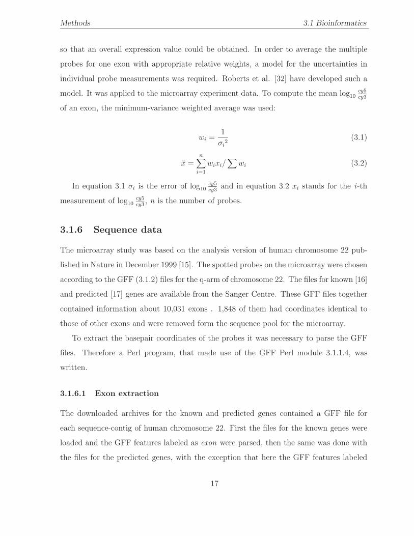
of an exon, the minimum-variance weighted average was used:

wi =1

σi2

(3.1)

x =n∑

i=1

wixi/∑

wi (3.2)

In equation 3.1 σi is the error of log10cy5cy3

and in equation 3.2 xi stands for the i -th

measurement of log10cy5cy3

, n is the number of probes.

3.1.6 Sequence data

The microarray study was based on the analysis version of human chromosome 22 pub-

lished in Nature in December 1999 [15]. The spotted probes on the microarray were chosen

according to the GFF (3.1.2) files for the q-arm of chromosome 22. The files for known [16]

and predicted [17] genes are available from the Sanger Centre. These GFF files together

contained information about 10,031 exons . 1,848 of them had coordinates identical to

those of other exons and were removed form the sequence pool for the microarray.

To extract the basepair coordinates of the probes it was necessary to parse the GFF

files. Therefore a Perl program, that made use of the GFF Perl module 3.1.1.4, was

written.

3.1.6.1 Exon extraction

The downloaded archives for the known and predicted genes contained a GFF file for

each sequence-contig of human chromosome 22. First the files for the known genes were

loaded and the GFF features labeled as exon were parsed, then the same was done with

the files for the predicted genes, with the exception that here the GFF features labeled

17

Methods 3.1 Bioinformatics

as CDS were extracted. The acquired features were then merged and sorted ascending

according to the start positions of the extracted exons. The obtained data included the

contig name, the start and end base position of the exon and the DNA-strand of the

coding sequences. Each exon found this way was given a unique id (E ID). Furthermore

the index number of the exon (Exon Nr) on a particular contig was determined simply by

counting the exons on it. The length of an exon was calculated by subtracting the start

position from the end position and adding 1. The Perl program produced a sorted and

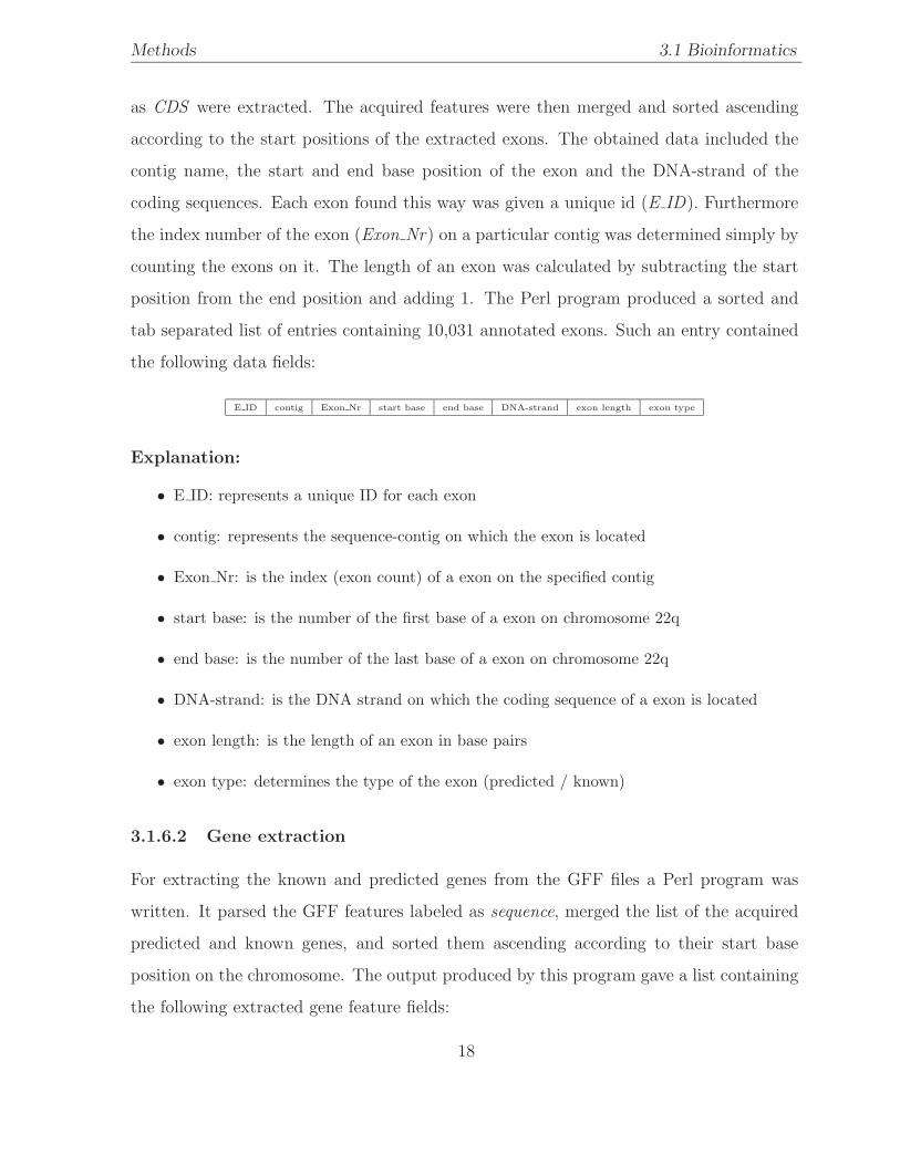
tab separated list of entries containing 10,031 annotated exons. Such an entry contained

the following data fields:

E ID contig Exon Nr start base end base DNA-strand exon length exon type

Explanation:

• E ID: represents a unique ID for each exon

• contig: represents the sequence-contig on which the exon is located

• Exon Nr: is the index (exon count) of a exon on the specified contig

• start base: is the number of the first base of a exon on chromosome 22q

• end base: is the number of the last base of a exon on chromosome 22q

• DNA-strand: is the DNA strand on which the coding sequence of a exon is located

• exon length: is the length of an exon in base pairs

• exon type: determines the type of the exon (predicted / known)

3.1.6.2 Gene extraction

For extracting the known and predicted genes from the GFF files a Perl program was

written. It parsed the GFF features labeled as sequence, merged the list of the acquired

predicted and known genes, and sorted them ascending according to their start base

position on the chromosome. The output produced by this program gave a list containing

the following extracted gene feature fields:

18

Methods 3.1 Bioinformatics

G ID contig Gene Nr start base end base DNA-strand gene length gene name description gene type

Explanation:

• G ID: represents a unique ID for each gene

• contig: represents the sequence-contig on which the gene is located

• Gene Nr: is the index (gene count) of a gene on the specified contig

• start base: is the number of the first base of a gene on chromosome 22q

• end base: is the number of the last base of a gene on chromosome 22q

• DNA-strand: is the DNA strand on which the coding sequence of a gene is located

• gene length: is the length of a gene in base pairs

• gene name: is the name of the coding sequence given in the GFF file

• description: is a short description of the coding sequence

• gene type: determines the type of the gene (predicted / known)

These lists could easily be imported into a relational database.

3.1.7 The database

To establish a connection between the expression data from the microarray and the posi-

tions of the single probes on the chromosome, a relational database model was developed.

3.1.7.1 Sequence data

The known and predicted exons of the q-arm of the chromosome (22q) were extracted

from the GFF files and led to the described lists.

A table for the sequence-contigs was created, where each of the contigs was entered with

a unique id C ID, the name of the contig Contig, the start and end base and its length.

A second table held the information about the exons extracted from the GFF files (see

19

Methods 3.1 Bioinformatics

3.1.6.1). The table was linked to the contig table over the contig id C ID, so that for

each exon the sequence-contig could be identified by following this link. The data fields

resulting from the gene extraction (see 3.1.6.2) were entered into their own table. This

table was also connected with the C ID to the contig table. The connection between

genes and exons was established by a ”map table”, where for each exon id (E ID) the

corresponding gene id (G ID) was entered.

3.1.7.2 Gene expression data

The descriptions of the 69 experiments were put into a table, where each experiment got

a unique id (X ID). The experiments were done with two differently designed slides, so

that the information about the used slide (Slide Set) was entered as well.

Each probe from the two different slides was extracted from the GEMLTM files and en-

tered into a table with a unique id (P ID), the slideset id (Slide Set) and the feature

number (F ID) on the microarray. The connection between exons and probes was real-

ized through the exon id E ID, which links a probe to an exon in the Exons table.

The expression data, which resulted from the microarray experiments, was entered in its

own table. It included the following fields for each probe: raw and normalized values

for both channels (cy3, cy5), log10cy5cy3

, σlog10cy5cy3

and XDEV. These values could be linked

through the probe id P ID to the corresponding probe in the Probes table and through

the X ID to the experiment from which the data originate. The same schema was used

for the reversed fluor experiments.

Since there were multiple probes for a single exon on the microarrays, the average (mean)

of the intensities of all probes on an exon were calculated and listed in the table Exon Expression.

Also an error weighted log cy5cy3

(see 3.1.5.2) of all probes belonging to an exon was entered

there.

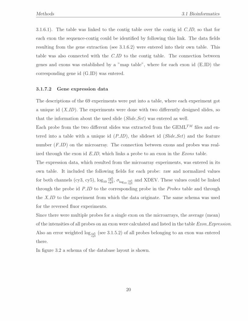
In figure 3.2 a schema of the database layout is shown.

20

Methods 3.1 Bioinformatics

Figure 3.2: Data model. shown are the tables of the database, connecting lines represent constrains

3.1.8 The scoring system

In order to find regions on the chromosome where there are significant differences in gene

expression between two different cell lines, a scoring system was developed.

The start and end (borders) of such regions were determined by a set of 22 bacterial

artificial chromosomes (BACs ), that have previously been mapped cytogenetically by

FISH to chromosome 22 (see 3.2). This BAC set is part of the FISH-mapped BACs

from the ”Cancer Chromosome Aberration Project” (Ccap) [52, 10]. In this project a

high-resolution fluorescence in situ hybridization (FISH) mapping of colony-purified BAC

clones, spaced at 1 to 2 Mbp intervals across the entire genome, was done.

The available sequences (BAC-end sequences, STS, entire sequences) of the BACs were

21

Methods 3.1 Bioinformatics

downloaded from GeneBank (http://www.ncbi.nlm.nih.gov) and mapped to the sequence

of the q-arm of human chromosome 22 [15] . The mapping was done with the megablast

program from NCBI (see 3.1.4).

With the scoring system the 21 resulting regions (each defined by the start- and end

position of two neighboring BACs) were scored with regard to the difference in the ex-

pression levels, the number and the length of the genes within such a region. The score

is influenced by the mean log10 of the expression ratio of the known and predicted exons

on a gene in the region, the mean log10 of the intensities of the spots of the exons on a

gene on the microarray, and the lengths of the different genes in the region. The first

two parameters take the difference in the expression level into account. The length of a

gene determines the size of the DNA piece over which the RNA-polymerase passes during

transcription, and thus the size of potential open chromatin.

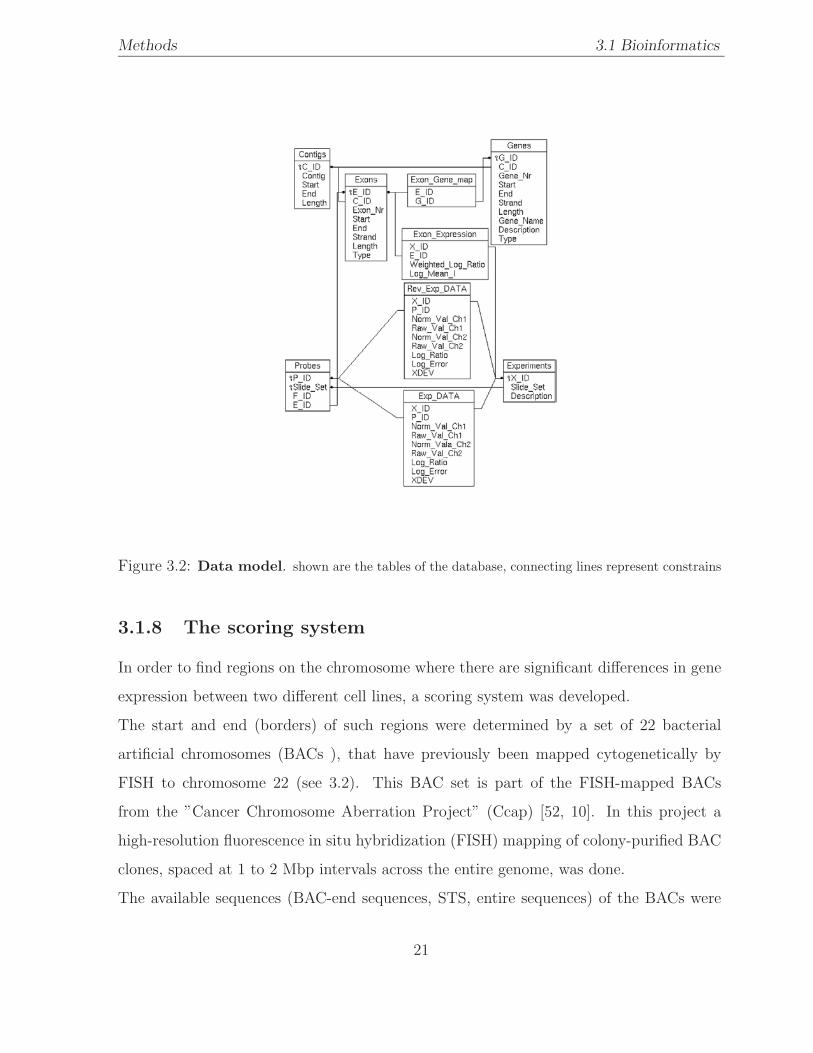
3.1.8.1 The algorithm

For the scoring a Perl-program was written. It fetched the expression data, using the

DBI (see 3.1.1.1), from the relational database system (MySQL) where the results of the

microarray experiments were stored. The program incorporated the following algorithm :

for all genes in region do

for all exons on currentgene do

if log10cy5cy3 ≥ ratio threshold AND log10 spot intensity ≥ intensity threshold then

upreg gene score = upreg gene score + ((log10 spot intensity + 2) ∗ log10cy5cy3 )

increaseupreg gen countby1

else if log10cy5cy3 ≤ −ratio threshold AND log10 spot intensity ≥ intensity threshold then

downreg gene score = downreg gene score + ((log10 spot intensity + 2) ∗ log10cy5cy3 )

increasedownreg gen countby1

end if

end for

upreg gene score = upreg gene score/upreg gen count

downreg gene score = downreg gene score/downreg gen count

if upreg gene score + downreg gene score ≥ (intensity threshold + 2) ∗ ratio threshold then

gene score = (upreg gene score + downreg gene score) ∗ gene length

end if

if upreg gene score + downreg gene score < (intensity threshold + 2) ∗ −(ratio threshold) then

gene score = (upreg gene score + downreg gene score) ∗ gene length

end if

score = score + gene score

end for

22

Methods 3.1 Bioinformatics

Explanation: Each exon on a gene which showed an expression ratio (log10cy5cy3

) and

a spot intensity on the microarray (log10 spot intensity) beyond certain thresholds was

considered as significantly up- or downregulated. For the expression ratio thresholds

(ratio threshold) 0.3 and -0.3 was used in this work - this represents a 2-fold up- or

downregulation of the exon in one cell line. The threshold for the spot intensity (inten-

sity threshold), which correlates to the amount of RNA, was -0.7. Below this threshold

errors tend to increase rapidly because spot intensities are not sufficiently above back-

ground intensity, therefore the values were not considered reliable [26].

For each of the up- or downregulated exons on a gene, an intermediate score (upreg gene score,

downreg gene score) was calculated. For doing this the values for the intensities were

first corrected by 2, to always get positive values. Then the corrected intensity value

was multiplied by the expression ratio value. These intermediate scores for the upregu-

lated exons were summed up and divided by the number of the exons on the gene. The

same was done for the downregulated exons. These two mean values (upreg gene score

and downreg gene score) were then summed up and multiplied by the length (in bases)

of the gene. This resulted in another intermediate score (=gene score) which repre-

sents a score for a single gene. The score for a gene was only considered as signifi-

cant if the sum upreg gene score + downreg gene score was bigger or smaller then the

threshold of (intensity threshold + 2) ∗ ratio threshold or (intensity threshold + 2) ∗−(ratio threshold) respectively. The significant gene scores of a region were then summed

up to come to the total score for the region.

3.1.9 Visualization of exon expression

To visualize the expression of the exons in the 21 different regions on human chromosome

22, a scatter plot for each region was created using the Chart::Plot, GD and DBI Perl

modules.

The log10 of the expression ratio for each exon in a particular region was plotted against

the log10 of the mean intensity of each exon. The resulting plots illustrate an expression

23

Methods 3.2 Microscopy: FISH

profile for each region. The study of these profiles in combination with the calculated

scores helped to find regions of interest.

3.2 Microscopy: FISH

With the above described methods it was possible to find transcriptional highly active,

and thus interesting regions on human chromosome 22. These regions should also show

a different structure in the chromatin, compared to a region with low transcriptional ac-

tivity [46, 19]. The structure of the chromatin in such a region should be visualized with

the help of fluorescence microscopy, using the DNA FISH method.

In situ hybridization (ISH ), is a method of localizing, either mRNA within the cy-

toplasm or DNA within the chromosomes of the nucleus, by hybridizing the sequence of

interest to a complementary strand of a nucleotide probe. Normal hybridization requires

the isolation of DNA or RNA, separating it on a gel, blotting it onto nitrocellulose and

probing it with a complementary sequence.

The basic principles for in situ hybridization are the same, except one is utilizing the

probe to detect specific nucleotide sequences within cells and tissues. It is presently used

by many laboratories for diagnosis of infectious diseases and cytogenetic analyses, as well

as for basic cell biology research to study structural and dynamic properties of tissues,

cells, and subcellular entities [23].

Probe sequences can be labeled with isotopes, but an increasing number of groups have

turned to nonisotopic in situ hybridization. It is faster, has a greater resolution, and

provides many options to simultaneously visualize different targets by combining various

detection methods [41]. The most popular ISH protocol utilizes fluorescence detection

and is therefore also known as FISH.

Nonisotopic labels include enzymes, haptens such as biotin or digoxigenin, and fluo-

rochromes. Usually, FISH is performed with biotinylated or digoxigenin-labeled probes

24

Methods 3.2 Microscopy: FISH

detected via fluorochrome-conjugated detection reagent, such as an antibody, or hapten-

specific reactive compounds, such as avidin or streptavidin when biotin is incorporated.

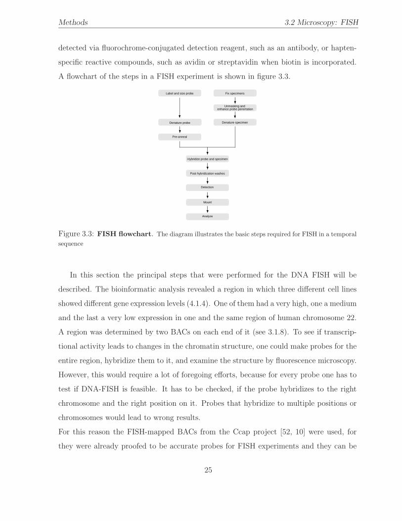
A flowchart of the steps in a FISH experiment is shown in figure 3.3.

Label and size probe Fix specimens

Unmasking and enhance probe penertation

Denature specimenDenature probe

Pre-anneal

Hybridize probe and specimen

Post-hybridization washes

Detection

Mount

Analyze

Figure 3.3: FISH flowchart. The diagram illustrates the basic steps required for FISH in a temporalsequence

In this section the principal steps that were performed for the DNA FISH will be

described. The bioinformatic analysis revealed a region in which three different cell lines

showed different gene expression levels (4.1.4). One of them had a very high, one a medium

and the last a very low expression in one and the same region of human chromosome 22.

A region was determined by two BACs on each end of it (see 3.1.8). To see if transcrip-

tional activity leads to changes in the chromatin structure, one could make probes for the

entire region, hybridize them to it, and examine the structure by fluorescence microscopy.

However, this would require a lot of foregoing efforts, because for every probe one has to

test if DNA-FISH is feasible. It has to be checked, if the probe hybridizes to the right

chromosome and the right position on it. Probes that hybridize to multiple positions or

chromosomes would lead to wrong results.

For this reason the FISH-mapped BACs from the Ccap project [52, 10] were used, for

they were already proofed to be accurate probes for FISH experiments and they can be

25

Methods 3.2 Microscopy: FISH

purchased from ResGen (Invitrogen Corporation). The BACs covered just the beginning

and the end of a region, so that for identifying changes in the chromatin structure, such

as decondensation and recondensation, the distance between the two has to be measured.

In case of a large scale decondensation of the chromatin, caused by transcription, one

would expect an increased distance between the two BACs. In the cell line for which

the microarray analysis revealed a low transcriptional activity, a condensed state of the

chromatin is predicted, thus the distance between the two BACs at the ends of the region

should be smaller.

Lawrence and colleges [22] could already show that it is possible to hybridize two probes,

spaced by ∼1Mbp, to an interphase chromosome and produce two distinct fluorescent

signals, of which the distance can be measured. This gave confidence that this approach

may have success in terms of identifying changes in large-scale chromatin structure.

To test if open structures are caused by transcriptional activity, the cells were treated

with 5,6-dichloro-1-β-D-ribofuranosylbenzimidazole (DRB ), a protein kinase inhibitor

that blocks the transition from polymerase II initiation to elongation [12]. The chromatin

structure of the DRB treated cells was then studied by DNA FISH.

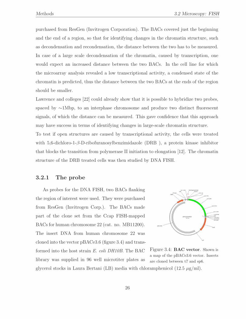
3.2.1 The probe

As probes for the DNA FISH, two BACs flanking

Figure 3.4: BAC vector. Shown isa map of the pBACe3.6 vector. Insertsare cloned between t7 and sp6.

the region of interest were used. They were purchased

from ResGen (Invitrogen Corp.). The BACs made

part of the clone set from the Ccap FISH-mapped

BACs for human chromosome 22 (cat. no. MB11200).

The insert DNA from human chromosome 22 was

cloned into the vector pBACe3.6 (figure 3.4) and trans-

formed into the host strain E. coli DH10B. The BAC

library was supplied in 96 well microtiter plates as

glycerol stocks in Laura Bertani (LB) media with chloramphenicol (12.5 µg/ml).

26

Methods 3.2 Microscopy: FISH

3.2.1.1 BAC isolation

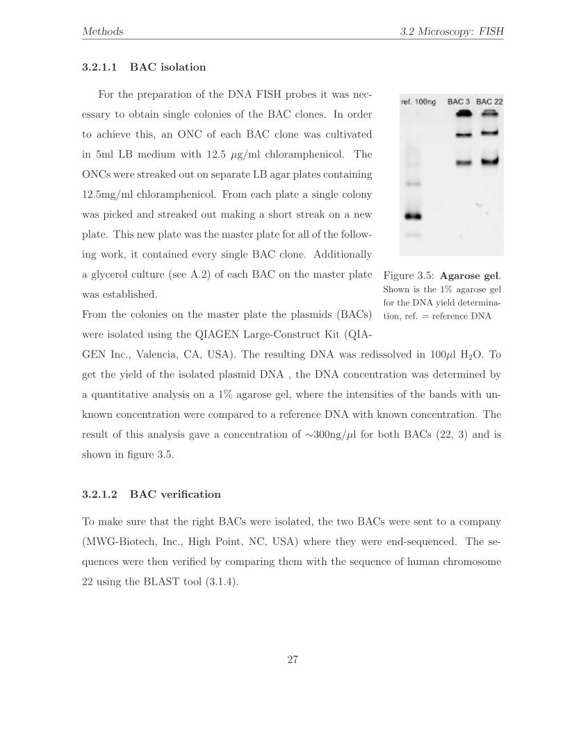
For the preparation of the DNA FISH probes it was nec-

Figure 3.5: Agarose gel.Shown is the 1% agarose gelfor the DNA yield determina-tion, ref. = reference DNA

essary to obtain single colonies of the BAC clones. In order

to achieve this, an ONC of each BAC clone was cultivated

in 5ml LB medium with 12.5 µg/ml chloramphenicol. The

ONCs were streaked out on separate LB agar plates containing

12.5mg/ml chloramphenicol. From each plate a single colony

was picked and streaked out making a short streak on a new

plate. This new plate was the master plate for all of the follow-

ing work, it contained every single BAC clone. Additionally

a glycerol culture (see A.2) of each BAC on the master plate

was established.

From the colonies on the master plate the plasmids (BACs)

were isolated using the QIAGEN Large-Construct Kit (QIA-

GEN Inc., Valencia, CA, USA). The resulting DNA was redissolved in 100µl H2O. To

get the yield of the isolated plasmid DNA , the DNA concentration was determined by

a quantitative analysis on a 1% agarose gel, where the intensities of the bands with un-

known concentration were compared to a reference DNA with known concentration. The

result of this analysis gave a concentration of ∼300ng/µl for both BACs (22, 3) and is

shown in figure 3.5.

3.2.1.2 BAC verification

To make sure that the right BACs were isolated, the two BACs were sent to a company

(MWG-Biotech, Inc., High Point, NC, USA) where they were end-sequenced. The se-

quences were then verified by comparing them with the sequence of human chromosome

22 using the BLAST tool (3.1.4).

27

Methods 3.2 Microscopy: FISH

3.2.1.3 Biotin-Nick translation

To generate biotin labeled probes a biotin nick translation [31]

was performed using the Biotin-Nick Translation Mix from

Boehringer Mannheim (cat. no. 17452824).

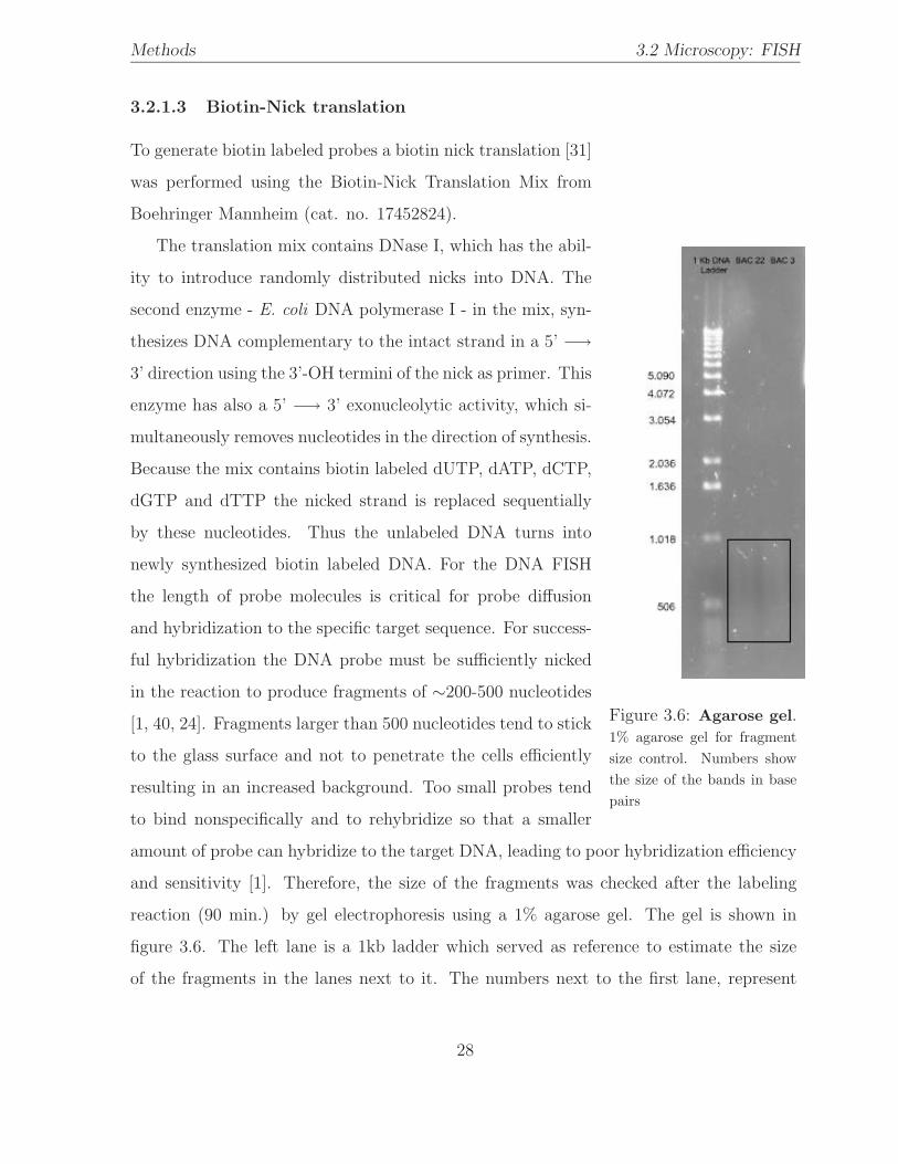
The translation mix contains DNase I, which has the abil-

Figure 3.6: Agarose gel.1% agarose gel for fragmentsize control. Numbers showthe size of the bands in basepairs

ity to introduce randomly distributed nicks into DNA. The

second enzyme - E. coli DNA polymerase I - in the mix, syn-

thesizes DNA complementary to the intact strand in a 5’ −→3’ direction using the 3’-OH termini of the nick as primer. This

enzyme has also a 5’ −→ 3’ exonucleolytic activity, which si-

multaneously removes nucleotides in the direction of synthesis.

Because the mix contains biotin labeled dUTP, dATP, dCTP,

dGTP and dTTP the nicked strand is replaced sequentially

by these nucleotides. Thus the unlabeled DNA turns into

newly synthesized biotin labeled DNA. For the DNA FISH

the length of probe molecules is critical for probe diffusion

and hybridization to the specific target sequence. For success-

ful hybridization the DNA probe must be sufficiently nicked

in the reaction to produce fragments of ∼200-500 nucleotides

[1, 40, 24]. Fragments larger than 500 nucleotides tend to stick

to the glass surface and not to penetrate the cells efficiently

resulting in an increased background. Too small probes tend

to bind nonspecifically and to rehybridize so that a smaller

amount of probe can hybridize to the target DNA, leading to poor hybridization efficiency

and sensitivity [1]. Therefore, the size of the fragments was checked after the labeling

reaction (90 min.) by gel electrophoresis using a 1% agarose gel. The gel is shown in

figure 3.6. The left lane is a 1kb ladder which served as reference to estimate the size

of the fragments in the lanes next to it. The numbers next to the first lane, represent

28

Methods 3.2 Microscopy: FISH

the size of the bands. The light smear in the box represents the fragment distribution.

As one can see, the size of the fragments ranges from ∼1000 to 300 bases, therefore the

nick translation was extended for 15 minutes in order to obtain fragments in the range of

∼200-500 nucleotides. After the labeling reaction the probe DNA was precipitated and

redissolved in 20µl H2O.

3.2.1.4 Probe preparation for in situ hybridization

After the biotin-nick translation further preparation steps are required.

Large probes often contain interspersed repetitive sequences (IRS ) that can cause back-

ground staining, because of the wide distribution of these sequences throughout the

genome. To prevent binding of labeled IRS within the probe to sequences other than

the targeted locus, chromosomal in situ suppression hybridization (CISS ) [24] was per-

formed. In this method competitor DNAs , COT-1 from Invitrogen (Invitrogen Corpora-

tion, Carlsbad, California 92008, cat. no. 15278-011) and salmon sperm DNA (Invitrogen,

cat. no. 15632-011), are used in a preannealing step. COT-1 DNA is obtained from hu-

man placental DNA and is rich in repetitive sequences, which can mask the IRS on the

probe. Salmon sperm DNA shares certain repetitive DNA elements in common with hu-

man DNA. It also prevents nonspecific binding of the hybridization-probe to the glass

surface of the coversilp used for FISH. Salmon sperm DNA acts also as carrier.

Briefly, biotinylated DNA (150 ng), COT-1 DNA (5 µg) and salmon sperm DNA (7 µg)

were combined in the hybridization solution and precipitated with 110

vol. 3M sodium

acetate pH 5.2 and 2 vol. abs. EtOH at −80◦C. After precipitating, the DNA was washed

with 70% EtOH, dried and redissolved in 2.5 µl formamide and 1 µl H2O at 37◦C for

20 minutes. 0.5 µl 20xSSC and 1 µl 25% dextran sulfate were added. The hybridization

cocktail with final concentrations of 50% formamide and 2xSSC determines the strin-

gency of denaturation and renaturation. Stringency can be increased by either raising

the temperature, increasing the concentration of formamide, or decreasing the number of

monovalent cations (lowering the SSC concentration).

The probe was denaturated for 10 minutes at 85◦C and prehybridized for 20 minutes at

29

Methods 3.2 Microscopy: FISH

37◦C before applying it to a separately denatured specimen (see 3.2.2.6).

3.2.2 The specimens

The bioinformatic analysis revealed a region on human chromosome 22, in which three cell

lines showed a significant difference in their gene expression (see 4.1.4). This region was

flanked by two BACs (22, 3), which were used as probes (see 3.2.1). The cell line K-562

had the highest expression level, Raji had the lowest and Jurkat was in between of K-562

and Raji. The region should therefore show different levels of chromatin compaction in

these cell lines.

3.2.2.1 Cell cultures

The three cell lines were ordered from ATCC (American Type Culture Collection, Man-

assas, VA, USA) and cultured according to the procedures described in the product in-

formation sheet that comes with the cell lines.

Briefly, for K-562 (cat. no. CCL-243) the Iscove’s modified Dulbecco’s medium with 4

mM L-glutamine that is modified by ATCC to contain 1.5g/L sodium bicarbonate (cat.

no. 30-2005) was used. For Raji (cat. no. CCl-86) and Jurkat (cat. no. TIB-152)

the growth-medium was RPMI 1640 with 2mM L-glutamine that is modified by ATCC

to contain 10mM HEPES, 1mM sodium pyruvate, 2.4 g/L glucose and 1.5 g/L sodium

bicarbonate (cat. no. 30-2001). The medium was supplemented with 10% fetal bovine

serum (FBS) and 1% Penicillin/Streptomycin. The cells were grown in 75 cm2 culture

flasks (containing 12 ml of medium) at 37◦C in a 5% CO2 in air atmosphere. The cultures

were maintained by removing 6 ml of the culture suspension and addition of fresh medium

of the same volume. This was done on a daily basis.

3.2.2.2 Preparation of coverslips

For in situ hybridization, the cells of 6 ml cell suspension were collected by centrifugation

(10 min. 800 rpm) and resuspended in 1 ml of fresh medium. 60 µl of this suspension were

30

Methods 3.2 Microscopy: FISH

applied onto poly-L-lysine coated coverslips (BD Biosciences, Bedford, MA, USA, cat. no.

354085) and incubated for 1 hour at 37◦C. During this incubation the cells attached to

the coated coverslip. For the DRB treatment, 100 µg/ml DRB (Calbiochem, San Diego,

CA, USA, cat. no. 287891) was added to the cell suspension before incubation.

3.2.2.3 Cell fixation

To study the structure of chromosomal regions within nuclei by in situ hybridization,

it is mandatory that cells retain as much as possible of their in vivo morphology [45,

44, 24]. For preservation of the three-dimensional structure a fixation was performed

with paraformaldehyde . It has been shown, that such a fixation has a high degree of

preservation of the spatial arrangement of ∼1 Mbp chromatin domains [35].

The coverslip with the attached cells was shortly rinsed with PBS (without Ca and Mg

= PBS−−) to wash away the medium. After this washing step the cells were fixed by

incubating them in 3.5% paraformaldehyde in PBS−− at room temperature for 15 minutes.

3.2.2.4 Cell permeabilization

To enable labeled probes to enter the cell nucleus, it is necessary to permeabilize the cells.

This was achieved by a treatment with 0.5% Triton X-100 in PBS−−. After the fixation

step, the cells were washed 2 x 5 minutes with PBS−− and incubated for 10 minutes

at room temperature in the Triton X-100 solution. At low concentrations the detergent

efficiently solvates cellular membranes without disturbing protein-protein interactions.

3.2.2.5 RNase treatment

After permeabilizing, the cells were washed 3 x 5 minutes with PBS−−. To prevent

hybridization of the probe with RNA in the cells, the RNA was digested with RNase.

The coverslip was incubated for 20 minutes in a 25 µg/ml RNase in PBS−− solution at

room temperature, and washed 3 x 5 minutes with PBS−−.

31

Methods 3.2 Microscopy: FISH

3.2.2.6 DNA denaturation

The DNA within paraformaldehyde-fixed cells is denatured by heat in formamide . This

procedure produces homogeneously distributed single-stranded DNA.

Before denaturing, the cells were incubated for 1 minute in a denaturation buffer (70%

formamide in 2xSSC). Then the coverslip was placed upside-down on a preheated (85◦C)

slide with a drop of the denaturation buffer on it, and denatured at 85◦C. The temperature

and duration of the denaturation for the three different cell lines was determined by

trying different combinations of time and temperature, and by checking the amount of

fluorescence signals after hybridization with the probe. With the optimal condition ≥90%

of the cells on the coverslip had signals. For Raji and Jurkat the best condition was a

temperature of 85◦C and a duration of 5 minutes. For K-562 a duration of 3.5 minutes

at 85◦C was sufficient for the denaturation.

The cells were dehydrated for 4 minutes in 70% EtOH, 4 minutes in 90% EtOH and 4

minutes in absolute EtOH. After that the coverslip with the cells was air-dried.

3.2.3 Hybridization

During the hybridization , the probe penetrates the cells and anneals to the comple-

mentary sequence on the denatured chromosome. The stringency of the annealing is

determined by the composition of the hybridization cocktail (see 3.2.1.4).

The prepared probe (see 3.2.1.4) was applied to a slide, the coverslip with the denatured

cells (see 3.2.2.6) was placed upside-down onto the probe and sealed with rubber cement.

The hybridization was performed at 37◦C in a moist chamber for ∼16 hours.

Posthybridization washes remove the nonspecifically bound probe and thus reduce the

background staining. Furthermore, the stringency of the FISH can be adjusted by posthy-

bridization washes. Therefore the coverslip was washed as follows after hybridization: 2

x 15 min. in 50% formamide in 2xSSC at 45◦C, 10 min. in 0.1xSSC, 10 min. in 2xSSC,

5 min. with 4xSSC.

32

Methods 3.2 Microscopy: FISH

3.2.4 Detection

To detect the hybridized labeled probe, the coverslip was incubated for 45 minutes with

5 µg/ml NeutrAvidin-Tetramethylrhodamine (Molecular Probes, Eugene, OR, USA, cat.

no. A-6373) in 4xSSC, 0.1% BSA and 0.01% Tween 20 (blocking solution).

Avidin has a high affinity for biotin and thus it binds to the hybridized biotinylated probe.

It is conjugated to tetramethylrhodamine, which absorbs light at a wavelength of 555 nm

and emits fluorescence at 580 nm. The blocking solution prevents nonspecific binding of

avidin [21].

The coverslip was washed once for 10 minutes in 4xSSC with 0.1% Tween 20, twice in

4xSSC for 10 minutes and once for 10 minutes in 2xSSC. After that it was placed into

PBS−−, where it could be stored at 4◦C for several days.

The samples were stained with the DNA fluorochrome DAPI (diamino phenylindole)

at a concentration of 0.2 µg/ml. The DNA FISH coverslips were examined on a Leica

DMRA upright microscope with a Leica 100x 1.3 NA oil immersion objective. Images were

collected with a Photometrics Sensys CCD camera with binning of one. This configuration

led to a resolution of 0.067 µm per pixel.

3.2.5 Measurements

To identify large scale chromatin decondensations, the distance between the two hy-

bridized probes was measured (see 3.2). The measurements were done with the Meta-

Morph Offline Version 4.6rs program package (Universal Imaging Corporation, Downing-

town, PA, USA).

For each hybridization experiment, images of ∼50 randomly selected cells were acquired

using an exposure time of 4 seconds. The background in the nuclei was subtracted and

the distance between the signals of the two BACs were measured by drawing a line from

the end of the first BAC to the end of the second. The number of the pixels of the result-

ing line was directly transformed into µm by multiplying them by 0.067. The data were

entered into a spreadsheet, for further analysis.

33

Methods 3.2 Microscopy: FISH

Individual BACs were measured, after background correction, by drawing a line that

follows the shape of the signal.

34

Chapter 4

Results

4.1 Bioinformatics

The first aim of this work was to find transcriptional highly active regions on a chromosome

in a natural system. In order to find such regions, an analysis of DNA microarrays

using bioinformatic methods was considered. In this section the results of this unbiased

approach are shown.

4.1.1 Microarray data

The search for public available microarray data, which covers an entire chromosome, re-

vealed a dataset that was produced by Shoemaker et. al. [34]. In this work the authors

used a microarray- based experimental method to validate predicted exons on human

chromosome 22. 8,183 annotated exons were monitored under different conditions. Specif-

ically, mRNAs from human cell lines and normal and diseased tissues were fluorescently

labeled with two different colors and hybridized in pairs to 69 individual chromosome 22

exon arrays.

The data was imported into a relational database and the expression data of each exon

was linked to a sequence position on the chromosome (see 3.1.7). The sequence positions

of the exons were extracted from GFF files, which contain the annotation of human chro-

35

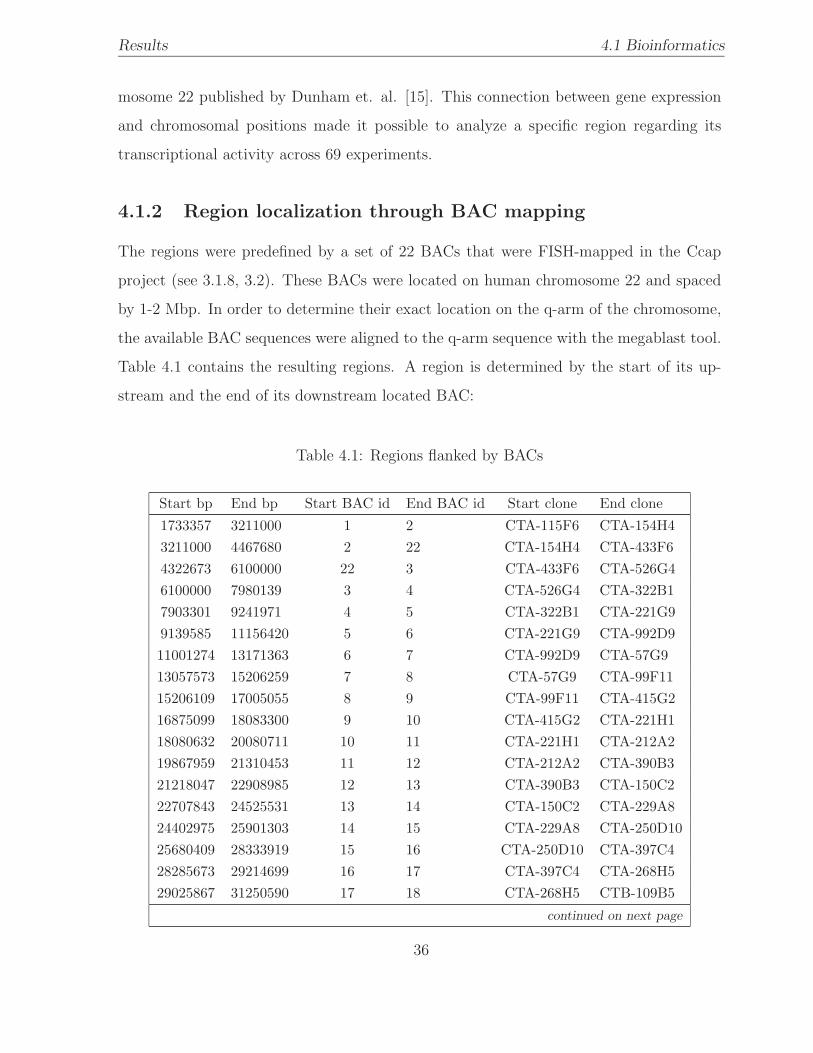
Results 4.1 Bioinformatics

mosome 22 published by Dunham et. al. [15]. This connection between gene expression

and chromosomal positions made it possible to analyze a specific region regarding its

transcriptional activity across 69 experiments.

4.1.2 Region localization through BAC mapping

The regions were predefined by a set of 22 BACs that were FISH-mapped in the Ccap

project (see 3.1.8, 3.2). These BACs were located on human chromosome 22 and spaced

by 1-2 Mbp. In order to determine their exact location on the q-arm of the chromosome,

the available BAC sequences were aligned to the q-arm sequence with the megablast tool.

Table 4.1 contains the resulting regions. A region is determined by the start of its up-

stream and the end of its downstream located BAC:

Table 4.1: Regions flanked by BACs

Start bp End bp Start BAC id End BAC id Start clone End clone

1733357 3211000 1 2 CTA-115F6 CTA-154H43211000 4467680 2 22 CTA-154H4 CTA-433F64322673 6100000 22 3 CTA-433F6 CTA-526G46100000 7980139 3 4 CTA-526G4 CTA-322B17903301 9241971 4 5 CTA-322B1 CTA-221G99139585 11156420 5 6 CTA-221G9 CTA-992D911001274 13171363 6 7 CTA-992D9 CTA-57G913057573 15206259 7 8 CTA-57G9 CTA-99F1115206109 17005055 8 9 CTA-99F11 CTA-415G216875099 18083300 9 10 CTA-415G2 CTA-221H118080632 20080711 10 11 CTA-221H1 CTA-212A219867959 21310453 11 12 CTA-212A2 CTA-390B321218047 22908985 12 13 CTA-390B3 CTA-150C222707843 24525531 13 14 CTA-150C2 CTA-229A824402975 25901303 14 15 CTA-229A8 CTA-250D1025680409 28333919 15 16 CTA-250D10 CTA-397C428285673 29214699 16 17 CTA-397C4 CTA-268H529025867 31250590 17 18 CTA-268H5 CTB-109B5

continued on next page

36

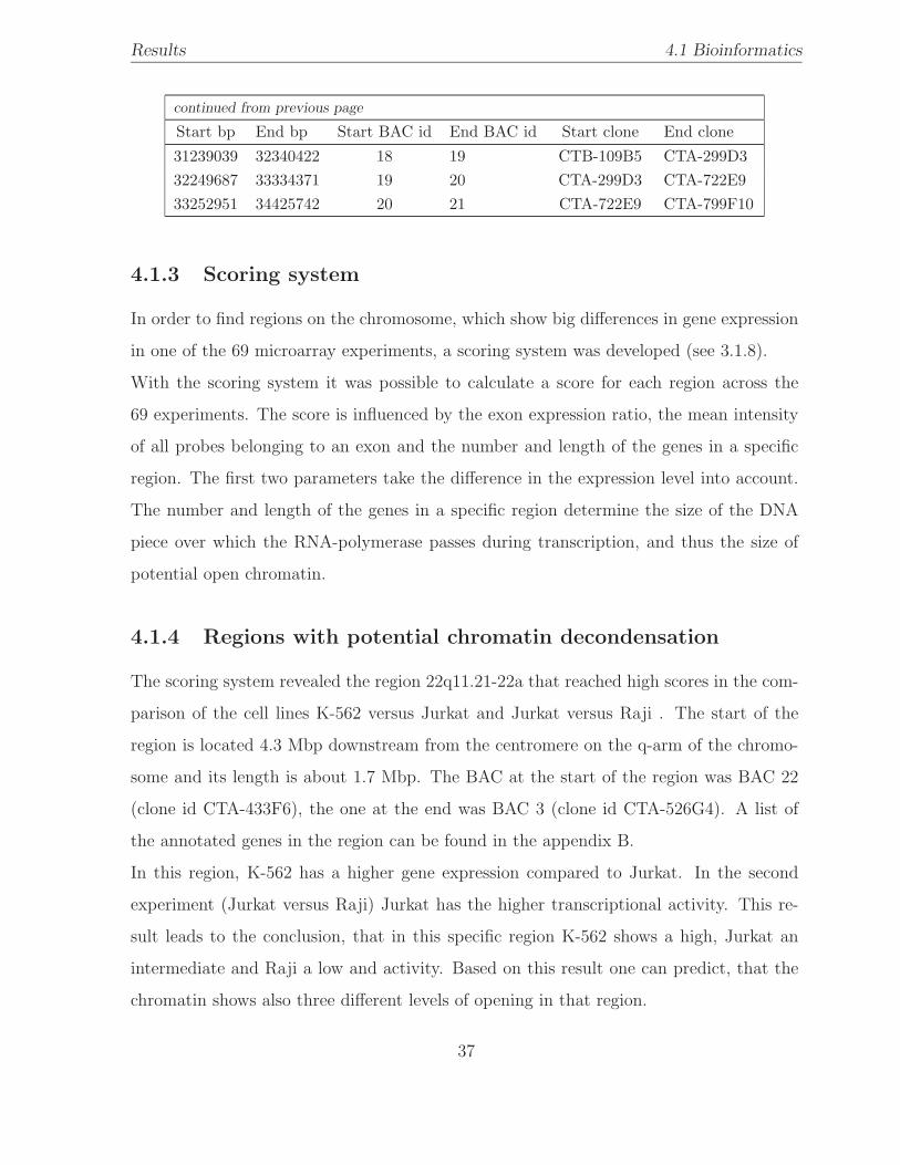
Results 4.1 Bioinformatics

continued from previous page

Start bp End bp Start BAC id End BAC id Start clone End clone

31239039 32340422 18 19 CTB-109B5 CTA-299D332249687 33334371 19 20 CTA-299D3 CTA-722E933252951 34425742 20 21 CTA-722E9 CTA-799F10

4.1.3 Scoring system

In order to find regions on the chromosome, which show big differences in gene expression

in one of the 69 microarray experiments, a scoring system was developed (see 3.1.8).

With the scoring system it was possible to calculate a score for each region across the

69 experiments. The score is influenced by the exon expression ratio, the mean intensity

of all probes belonging to an exon and the number and length of the genes in a specific

region. The first two parameters take the difference in the expression level into account.

The number and length of the genes in a specific region determine the size of the DNA

piece over which the RNA-polymerase passes during transcription, and thus the size of

potential open chromatin.

4.1.4 Regions with potential chromatin decondensation

The scoring system revealed the region 22q11.21-22a that reached high scores in the com-

parison of the cell lines K-562 versus Jurkat and Jurkat versus Raji . The start of the

region is located 4.3 Mbp downstream from the centromere on the q-arm of the chromo-

some and its length is about 1.7 Mbp. The BAC at the start of the region was BAC 22

(clone id CTA-433F6), the one at the end was BAC 3 (clone id CTA-526G4). A list of

the annotated genes in the region can be found in the appendix B.

In this region, K-562 has a higher gene expression compared to Jurkat. In the second

experiment (Jurkat versus Raji) Jurkat has the higher transcriptional activity. This re-

sult leads to the conclusion, that in this specific region K-562 shows a high, Jurkat an

intermediate and Raji a low and activity. Based on this result one can predict, that the

chromatin shows also three different levels of opening in that region.

37

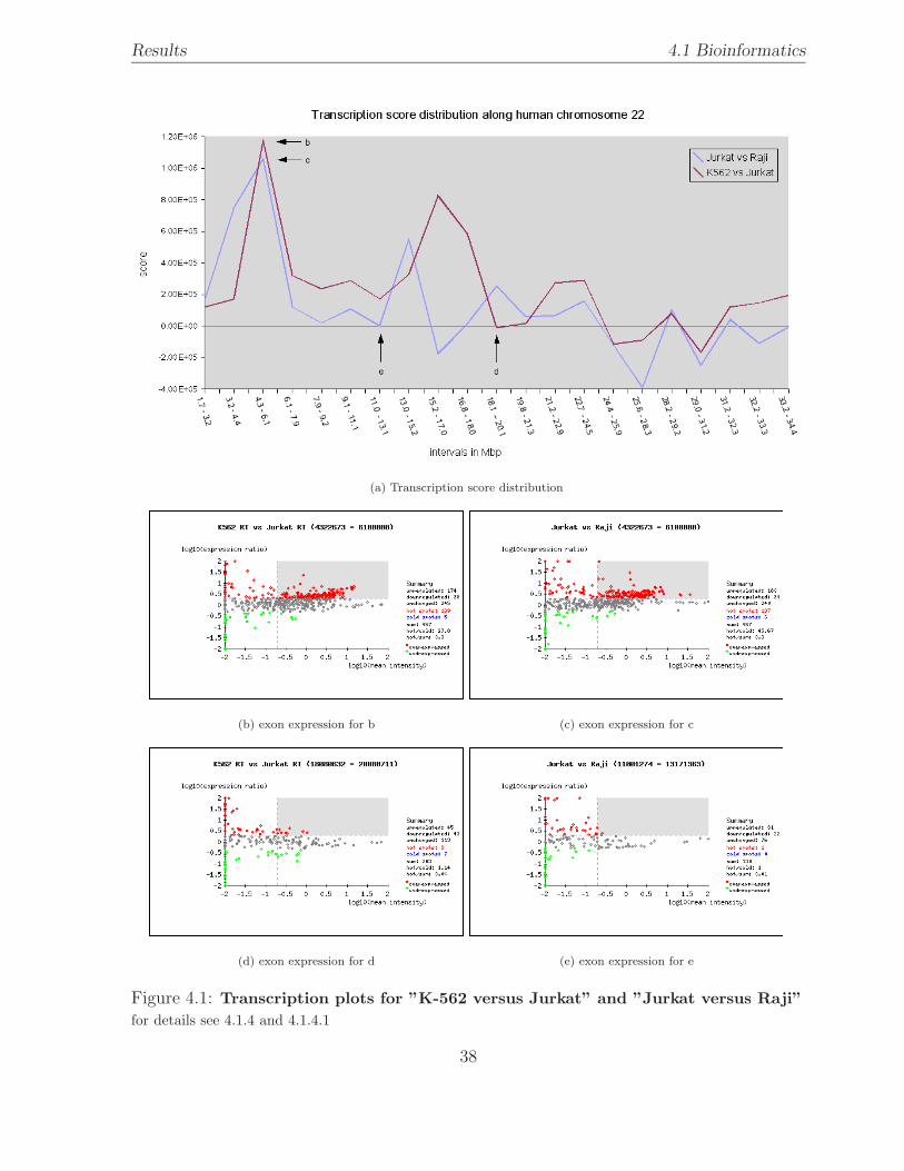
Results 4.1 Bioinformatics

(a) Transcription score distribution

(b) exon expression for b (c) exon expression for c

(d) exon expression for d (e) exon expression for e

Figure 4.1: Transcription plots for ”K-562 versus Jurkat” and ”Jurkat versus Raji”for details see 4.1.4 and 4.1.4.1

38

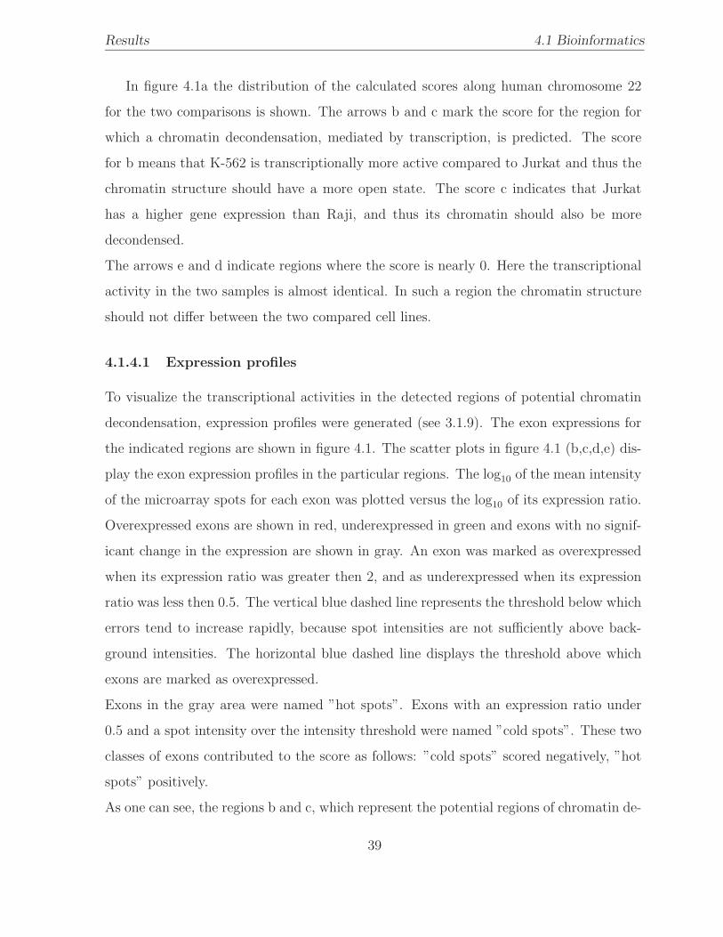
Results 4.1 Bioinformatics

In figure 4.1a the distribution of the calculated scores along human chromosome 22

for the two comparisons is shown. The arrows b and c mark the score for the region for

which a chromatin decondensation, mediated by transcription, is predicted. The score

for b means that K-562 is transcriptionally more active compared to Jurkat and thus the

chromatin structure should have a more open state. The score c indicates that Jurkat

has a higher gene expression than Raji, and thus its chromatin should also be more

decondensed.

The arrows e and d indicate regions where the score is nearly 0. Here the transcriptional

activity in the two samples is almost identical. In such a region the chromatin structure

should not differ between the two compared cell lines.

4.1.4.1 Expression profiles

To visualize the transcriptional activities in the detected regions of potential chromatin

decondensation, expression profiles were generated (see 3.1.9). The exon expressions for

the indicated regions are shown in figure 4.1. The scatter plots in figure 4.1 (b,c,d,e) dis-

play the exon expression profiles in the particular regions. The log10 of the mean intensity

of the microarray spots for each exon was plotted versus the log10 of its expression ratio.

Overexpressed exons are shown in red, underexpressed in green and exons with no signif-

icant change in the expression are shown in gray. An exon was marked as overexpressed

when its expression ratio was greater then 2, and as underexpressed when its expression

ratio was less then 0.5. The vertical blue dashed line represents the threshold below which

errors tend to increase rapidly, because spot intensities are not sufficiently above back-

ground intensities. The horizontal blue dashed line displays the threshold above which

exons are marked as overexpressed.

Exons in the gray area were named ”hot spots”. Exons with an expression ratio under

0.5 and a spot intensity over the intensity threshold were named ”cold spots”. These two

classes of exons contributed to the score as follows: ”cold spots” scored negatively, ”hot

spots” positively.

As one can see, the regions b and c, which represent the potential regions of chromatin de-

39

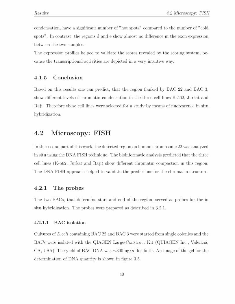
Results 4.2 Microscopy: FISH

condensation, have a significant number of ”hot spots” compared to the number of ”cold

spots”. In contrast, the regions d and e show almost no difference in the exon expression

between the two samples.

The expression profiles helped to validate the scores revealed by the scoring system, be-

cause the transcriptional activities are depicted in a very intuitive way.

4.1.5 Conclusion

Based on this results one can predict, that the region flanked by BAC 22 and BAC 3,

show different levels of chromatin condensation in the three cell lines K-562, Jurkat and

Raji. Therefore these cell lines were selected for a study by means of fluorescence in situ

hybridization.

4.2 Microscopy: FISH

In the second part of this work, the detected region on human chromosome 22 was analyzed

in situ using the DNA FISH technique. The bioinformatic analysis predicted that the three

cell lines (K-562, Jurkat and Raji) show different chromatin compaction in this region.

The DNA FISH approach helped to validate the predictions for the chromatin structure.

4.2.1 The probes

The two BACs, that determine start and end of the region, served as probes for the in

situ hybridization. The probes were prepared as described in 3.2.1.

4.2.1.1 BAC isolation

Cultures of E.coli containing BAC 22 and BAC 3 were started from single colonies and the

BACs were isolated with the QIAGEN Large-Construct Kit (QUIAGEN Inc., Valencia,

CA, USA). The yield of BAC DNA was ∼300 ng/µl for both. An image of the gel for the

determination of DNA quantity is shown in figure 3.5.

40

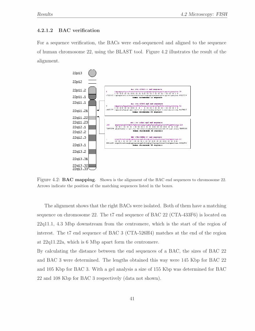
Results 4.2 Microscopy: FISH

4.2.1.2 BAC verification

For a sequence verification, the BACs were end-sequenced and aligned to the sequence

of human chromosome 22, using the BLAST tool. Figure 4.2 illustrates the result of the

alignment.

Figure 4.2: BAC mapping. Shown is the alignment of the BAC end sequences to chromosome 22.Arrows indicate the position of the matching sequences listed in the boxes.

The alignment shows that the right BACs were isolated. Both of them have a matching

sequence on chromosome 22. The t7 end sequence of BAC 22 (CTA-433F6) is located on

22q11.1, 4.3 Mbp downstream from the centromere, which is the start of the region of

interest. The t7 end sequence of BAC 3 (CTA-526H4) matches at the end of the region

at 22q11.22a, which is 6 Mbp apart form the centromere.

By calculating the distance between the end sequences of a BAC, the sizes of BAC 22

and BAC 3 were determined. The lengths obtained this way were 145 Kbp for BAC 22

and 105 Kbp for BAC 3. With a gel analysis a size of 155 Kbp was determined for BAC

22 and 108 Kbp for BAC 3 respectively (data not shown).

41

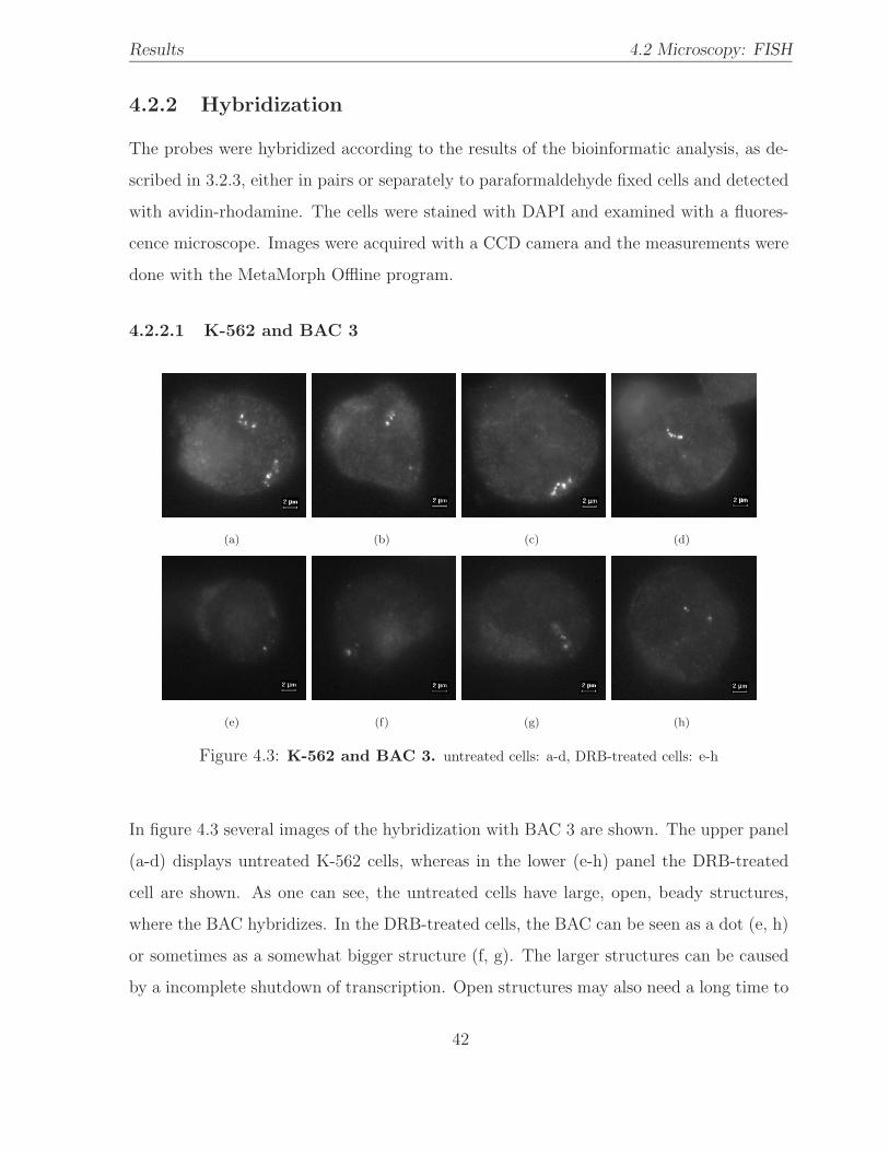
Results 4.2 Microscopy: FISH

4.2.2 Hybridization

The probes were hybridized according to the results of the bioinformatic analysis, as de-

scribed in 3.2.3, either in pairs or separately to paraformaldehyde fixed cells and detected

with avidin-rhodamine. The cells were stained with DAPI and examined with a fluores-

cence microscope. Images were acquired with a CCD camera and the measurements were

done with the MetaMorph Offline program.

4.2.2.1 K-562 and BAC 3

(a) (b) (c) (d)

(e) (f) (g) (h)

Figure 4.3: K-562 and BAC 3. untreated cells: a-d, DRB-treated cells: e-h

In figure 4.3 several images of the hybridization with BAC 3 are shown. The upper panel

(a-d) displays untreated K-562 cells, whereas in the lower (e-h) panel the DRB-treated

cell are shown. As one can see, the untreated cells have large, open, beady structures,

where the BAC hybridizes. In the DRB-treated cells, the BAC can be seen as a dot (e, h)

or sometimes as a somewhat bigger structure (f, g). The larger structures can be caused

by a incomplete shutdown of transcription. Open structures may also need a long time to

42

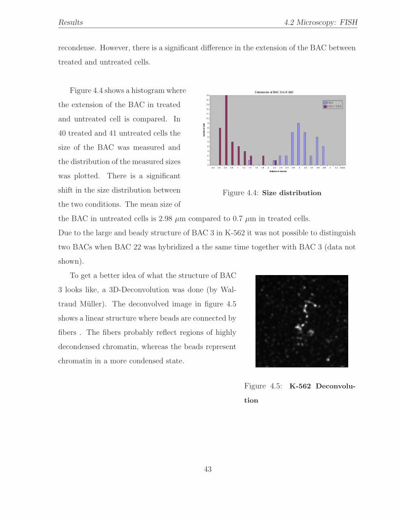
Results 4.2 Microscopy: FISH

recondense. However, there is a significant difference in the extension of the BAC between

treated and untreated cells.

Figure 4.4 shows a histogram where

Figure 4.4: Size distribution

the extension of the BAC in treated

and untreated cell is compared. In

40 treated and 41 untreated cells the

size of the BAC was measured and

the distribution of the measured sizes

was plotted. There is a significant

shift in the size distribution between

the two conditions. The mean size of

the BAC in untreated cells is 2.98 µm compared to 0.7 µm in treated cells.

Due to the large and beady structure of BAC 3 in K-562 it was not possible to distinguish

two BACs when BAC 22 was hybridized a the same time together with BAC 3 (data not

shown).

To get a better idea of what the structure of BAC

Figure 4.5: K-562 Deconvolu-

tion

3 looks like, a 3D-Deconvolution was done (by Wal-

traud Muller). The deconvolved image in figure 4.5

shows a linear structure where beads are connected by

fibers . The fibers probably reflect regions of highly

decondensed chromatin, whereas the beads represent

chromatin in a more condensed state.

43

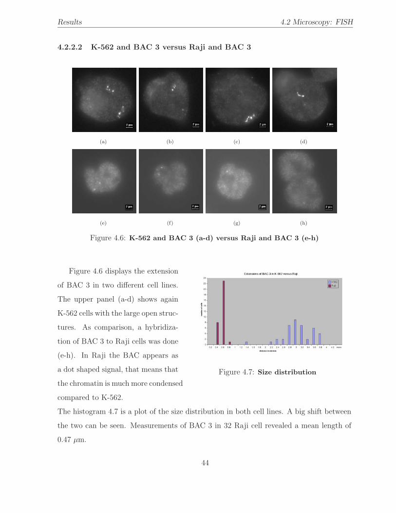
Results 4.2 Microscopy: FISH

4.2.2.2 K-562 and BAC 3 versus Raji and BAC 3

(a) (b) (c) (d)

(e) (f) (g) (h)

Figure 4.6: K-562 and BAC 3 (a-d) versus Raji and BAC 3 (e-h)

Figure 4.6 displays the extension

Figure 4.7: Size distribution

of BAC 3 in two different cell lines.

The upper panel (a-d) shows again

K-562 cells with the large open struc-

tures. As comparison, a hybridiza-

tion of BAC 3 to Raji cells was done

(e-h). In Raji the BAC appears as

a dot shaped signal, that means that

the chromatin is much more condensed

compared to K-562.

The histogram 4.7 is a plot of the size distribution in both cell lines. A big shift between

the two can be seen. Measurements of BAC 3 in 32 Raji cell revealed a mean length of

0.47 µm.

44

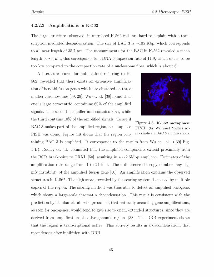
Results 4.2 Microscopy: FISH

4.2.2.3 Amplifications in K-562

The large structures observed, in untreated K-562 cells are hard to explain with a tran-

scription mediated decondensation. The size of BAC 3 is ∼105 Kbp, which corresponds

to a linear length of 35.7 µm. The measurements for the BAC in K-562 revealed a mean

length of ∼3 µm, this corresponds to a DNA compaction rate of 11.9, which seems to be

too low compared to the compaction rate of a nucleosome fiber, which is about 6.

A literature search for publications referring to K-

Figure 4.8: K-562 metaphaseFISH. (by Waltraud Muller) Ar-rows indicate BAC 3 amplifications.

562, revealed that there exists an extensive amplifica-

tion of bcr/abl fusion genes which are clustered on three

marker chromosomes [39, 29]. Wu et. al. [39] found that

one is large acrocentric, containing 60% of the amplified

signals. The second is smaller and contains 30%, while

the third contains 10% of the amplified signals. To see if

BAC 3 makes part of the amplified region, a metaphase

FISH was done. Figure 4.8 shows that the region con-

taining BAC 3 is amplified. It corresponds to the results from Wu et. al. ([39] Fig.

1 B). Rodley et. al. estimated that the amplified components extend proximally from

the BCR breakpoint to CRKL [50], resulting in a ∼2.5Mbp amplicon. Estimates of the

amplification rate range from 4 to 24 fold. These differences in copy number may sig-

nify instability of the amplified fusion gene [50]. An amplification explains the observed

structures in K-562. The high score, revealed by the scoring system, is caused by multiple

copies of the region. The scoring method was thus able to detect an amplified oncogene,

which shows a large-scale chromatin decondensation. This result is consistent with the

prediction by Tumbar et. al. who presumed, that naturally occurring gene amplifications,

as seen for oncogenes, would tend to give rise to open, extended structures, since they are

derived from amplification of active genomic regions [38]. The DRB experiment shows

that the region is transcriptional active. This activity results in a decondensation, that

recondenses after inhibition with DRB.

45

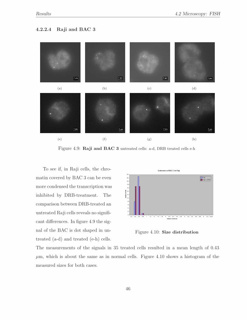
Results 4.2 Microscopy: FISH

4.2.2.4 Raji and BAC 3

(a) (b) (c) (d)

(e) (f) (g) (h)

Figure 4.9: Raji and BAC 3 untreated cells: a-d, DRB treated cells e-h

To see if, in Raji cells, the chro-

Figure 4.10: Size distribution

matin covered by BAC 3 can be even

more condensed the transcription was

inhibited by DRB-treatment. The

comparison between DRB-treated an

untreated Raji cells reveals no signifi-

cant differences. In figure 4.9 the sig-

nal of the BAC is dot shaped in un-

treated (a-d) and treated (e-h) cells.

The measurements of the signals in 35 treated cells resulted in a mean length of 0.43

µm, which is about the same as in normal cells. Figure 4.10 shows a histogram of the

measured sizes for both cases.

46

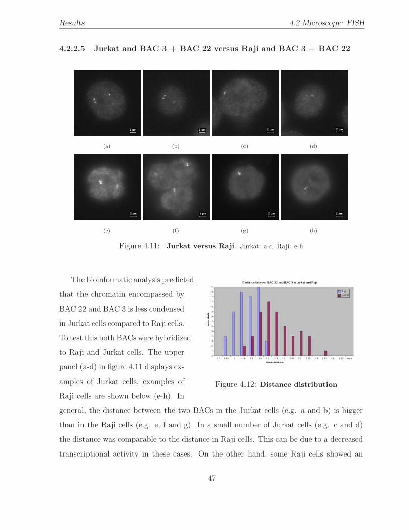
Results 4.2 Microscopy: FISH

4.2.2.5 Jurkat and BAC 3 + BAC 22 versus Raji and BAC 3 + BAC 22

(a) (b) (c) (d)

(e) (f) (g) (h)

Figure 4.11: Jurkat versus Raji. Jurkat: a-d, Raji: e-h

The bioinformatic analysis predicted

Figure 4.12: Distance distribution

that the chromatin encompassed by

BAC 22 and BAC 3 is less condensed

in Jurkat cells compared to Raji cells.

To test this both BACs were hybridized

to Raji and Jurkat cells. The upper

panel (a-d) in figure 4.11 displays ex-

amples of Jurkat cells, examples of

Raji cells are shown below (e-h). In

general, the distance between the two BACs in the Jurkat cells (e.g. a and b) is bigger

than in the Raji cells (e.g. e, f and g). In a small number of Jurkat cells (e.g. c and d)

the distance was comparable to the distance in Raji cells. This can be due to a decreased

transcriptional activity in these cases. On the other hand, some Raji cells showed an

47

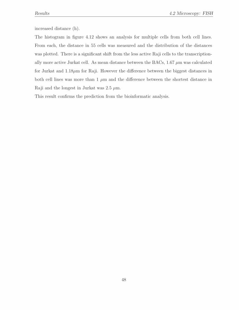
Results 4.2 Microscopy: FISH

increased distance (h).

The histogram in figure 4.12 shows an analysis for multiple cells from both cell lines.

From each, the distance in 55 cells was measured and the distribution of the distances

was plotted. There is a significant shift from the less active Raji cells to the transcription-

ally more active Jurkat cell. As mean distance between the BACs, 1.67 µm was calculated

for Jurkat and 1.18µm for Raji. However the difference between the biggest distances in

both cell lines was more than 1 µm and the difference between the shortest distance in

Raji and the longest in Jurkat was 2.5 µm.

This result confirms the prediction from the bioinformatic analysis.

48

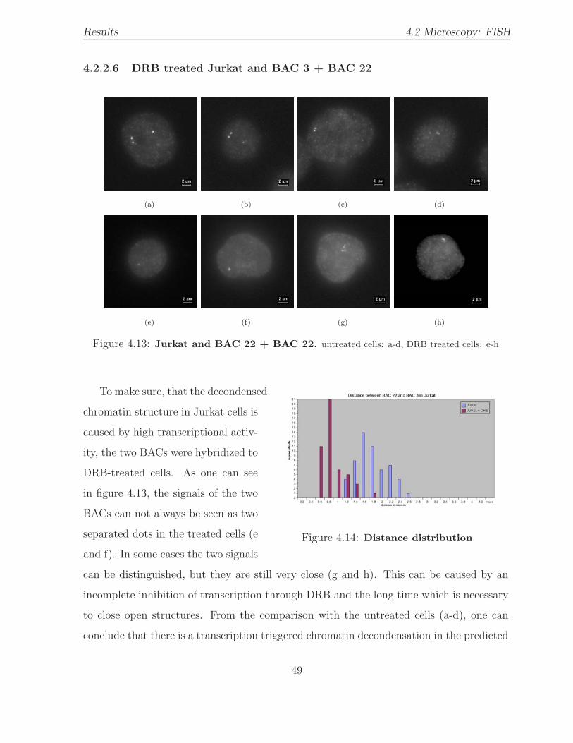
Results 4.2 Microscopy: FISH

4.2.2.6 DRB treated Jurkat and BAC 3 + BAC 22

(a) (b) (c) (d)

(e) (f) (g) (h)

Figure 4.13: Jurkat and BAC 22 + BAC 22. untreated cells: a-d, DRB treated cells: e-h

To make sure, that the decondensed

Figure 4.14: Distance distribution

chromatin structure in Jurkat cells is

caused by high transcriptional activ-

ity, the two BACs were hybridized to

DRB-treated cells. As one can see

in figure 4.13, the signals of the two

BACs can not always be seen as two

separated dots in the treated cells (e

and f). In some cases the two signals

can be distinguished, but they are still very close (g and h). This can be caused by an

incomplete inhibition of transcription through DRB and the long time which is necessary

to close open structures. From the comparison with the untreated cells (a-d), one can

conclude that there is a transcription triggered chromatin decondensation in the predicted

49

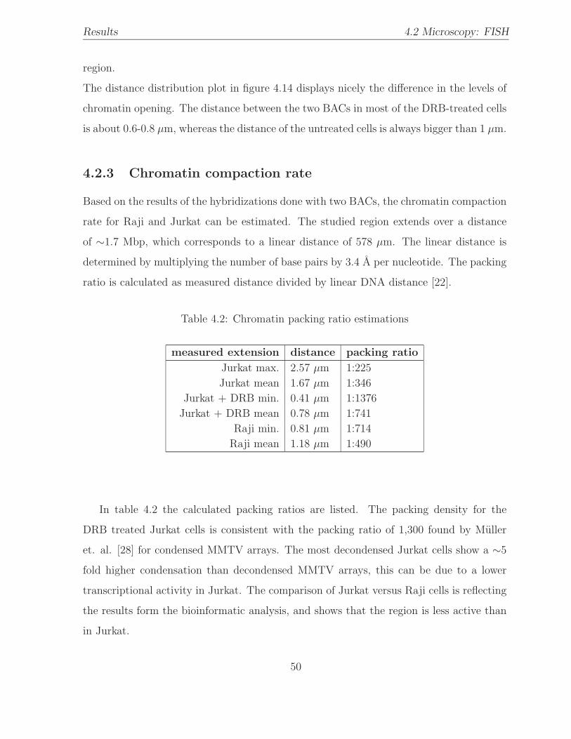
Results 4.2 Microscopy: FISH

region.

The distance distribution plot in figure 4.14 displays nicely the difference in the levels of

chromatin opening. The distance between the two BACs in most of the DRB-treated cells

is about 0.6-0.8 µm, whereas the distance of the untreated cells is always bigger than 1 µm.

4.2.3 Chromatin compaction rate

Based on the results of the hybridizations done with two BACs, the chromatin compaction

rate for Raji and Jurkat can be estimated. The studied region extends over a distance

of ∼1.7 Mbp, which corresponds to a linear distance of 578 µm. The linear distance is

determined by multiplying the number of base pairs by 3.4 A per nucleotide. The packing

ratio is calculated as measured distance divided by linear DNA distance [22].

Table 4.2: Chromatin packing ratio estimations

measured extension distance packing ratio

Jurkat max. 2.57 µm 1:225

Jurkat mean 1.67 µm 1:346

Jurkat + DRB min. 0.41 µm 1:1376

Jurkat + DRB mean 0.78 µm 1:741

Raji min. 0.81 µm 1:714

Raji mean 1.18 µm 1:490

In table 4.2 the calculated packing ratios are listed. The packing density for the

DRB treated Jurkat cells is consistent with the packing ratio of 1,300 found by Muller

et. al. [28] for condensed MMTV arrays. The most decondensed Jurkat cells show a ∼5

fold higher condensation than decondensed MMTV arrays, this can be due to a lower

transcriptional activity in Jurkat. The comparison of Jurkat versus Raji cells is reflecting

the results form the bioinformatic analysis, and shows that the region is less active than

in Jurkat.

50

Chapter 5

Discussion

The results of this work suggest that there exist active chromosomal regions which are

correlated with large-scale chromatin decondensations.

The bioinformatic analysis of human chromosome 22 microarray data [34], revealed a

region that shows different transcriptional activity in three different cell lines, namely K-

562, Jurkat and Raji. This region begins 4.3 Mbp apart from the centromere and extends

over 1.7 Mbp. In order to find out if this chromosomal region shows transcriptionally

mediated changes, such as decondensation, in its large-scale structure, it was investigated

by DNA-FISH. Two BAC probes (BAC 22 ∼ CTA-433F6, BAC 3 ∼ CTA-526G4) flanking

the region, were simultaneously hybridized to the interphase chromosomes of the three cell

lines. Changes in the large-scale structure were determined by measuring the distances

between the fluorescence signals of the two BACs. This approach was chosen, because of

the availability of already ”FISH-mapped” BACs [52, 10], that were proven to hybridize

to unambiguous positions on the chromosome and thus produce clear signals.

In K-562, the cell line that showed the highest transcriptional activity, it was not possible

to distinguish two signals, because BAC 3 produced very large linear and beady structures.

Thus this single BAC was examined further. Measurements of the extension of the BAC

in 40 cells revealed a mean length of ∼3 µm. A metaphase-FISH revealed, that the region

in which BAC 3 is located is amplified in K-562. This is consistent with previous studies

on this cell line [39, 29, 50], which revealed an extensive amplification of the bcr/abl

51

Discussion

oncogene. The long structures, that were observed, can be partially explained by this

amplification: The size of BAC 3 is 105 Kbp, that corresponds to a linear length of 35.7

µm. The measured extension of 3 µm means a chromatin compaction rate of ∼12, which is

too low compared to the compaction of the nucleosome fiber and compared to results from

previous work [28]. However, to see if also transcription was involved in the formation of

the observed structures the cells were treated with DRB, in order to inhibit transcription.

The images showed more compact fluorescent signals with a mean extension of ∼0.7 µm,

suggesting that a large-scale chromatin decondensation, caused by gene transcription,

occurs in the untreated cells. This result is consistent with a prediction by Tumbar et.

al., who presumed that large-scale openings in naturally occurring gene amplifications,

such as oncogenes, would tend to produce open structures [38].

In Jurkat and Raji it was possible to work with both BACs. The scoring system from the

bioinformatic analysis predicted that in Jurkat the distance between the two BACs would

be bigger than in Raji. This could be shown by DNA-FISH. The Jurkat cell line was

additionally, treated with DRB, in order to examine if the difference in the distances was

due to higher transcriptional activity. The treated cells again showed a recondensation of

the chromatin in the region, as indicated by the signals which consistently coincided or

overlapped.

The results of the FISH experiments lead to the conclusion, that it was possible to predict

and identify large-scale chromatin decondensations. Moreover the scoring system which

was developed for this work, found a region of an amplified oncogene. The overall results

are consistent with the ”chromonema fiber” model for higher order chromatin structure,

which implies the formation of decondensed fibers over a large range in active chromosomal

regions [6, 19]. The deconvolved images of the amplified BAC 3 give an additional clue

for the existence of such fibers.

As future aspect, a further investigation of the region with probes covering the entire

region would be of interest. The structure in between of the two BACs could then be

studied by 3D-deconvolution, which would help to get a better insight in the large-scale

chromatin organization.

52

Acknowledgments

I want to thank all my supporters, especially my supervisor Zlatko Trajanoski who gave

me the great opportunity to conduct the studies for my thesis at the National Institutes

of Health.

I want to express my honest gratitude to Waltraud Muller and James McNally who

conducted me through the work and from whom I learned a lot: ”It was a great honour

to work in your group!”

Special thanks go to my girlfriend Lisi for her love, patience and support during my

stay in the US.

Finally I want to thank my parents for their support and faith throughout my study.

53

Bibliography

[1] Boehringer Mannheim GMBH, Sandhofer Strasse 116, D-68305 Mannheim, Germany.

Biotin-Nick Translation Mix.

[2] CPAN: Comprehensive Perl Archive Network. WWW. http://www.cpan.org.

[3] Alberts Bruce; Bra Dennis; Lewis Julian; Raff Martin; Roberts Keith; Watson James

D.;. Molecular Biology of the Cell. Garland Publishing, 3rd edition, 1994.

[4] Stein L. D. GD.pm - Interface to Gd Graphics Library. WWW, 2000.

http://search.cpan.org/author/LDS/GD-2.01/GD.pm.

[5] Altschul S.F. et. al. Basic Local Alignment Search Tool. Journal of Molecular Biology,

215:403–410, October 1990.

[6] Belmont A. S. et. al. Visualization of G1 Chromosomes: A Folded, Twisted, Super-

coiled Chromonema Model of Interphase Chromatin Structure. The Journal of Cell

Biology, 127:287–302, October 1994.

[7] Belmont A. S. et. al. Large-scale chromatin sturcture and function. Current Opinion

in Cell Biology, 11:307–311, June 1999.

[8] Bunce T. et. al. DBI - Database independent interface for Perl. WWW, 2002.

http://search.cpan.org/author/TIMB/DBI-1.30/DBI.pm.

[9] Caron H. et al. The human transcriptome map: clustering of highly expressed genes

in chromosomal domains. Science, 291:1289–1292, February 2001.

54

BIBLIOGRAPHY BIBLIOGRAPHY

[10] Cheung V. G. et al. Integration of cytogenetic landmarks into the draft sequqnce of

the human genome. Nature, 409:953–958, February 2001.

[11] Cho R. J. et al. A genome-wide transcriptional analysis of the mitotic cell cycle.

Mol. Cell, 2:65–73, July 1998.

[12] Chodosh L.A. et. al. 5,6-dichloro-1-β-D-ribofuranosylbenzimidazole inhibits tran-

scription elongation by RNA polymerase II in vitro. Journal of Biological Chemistry,

264:2250–2257, February 1989.

[13] Cohen B. A. et. al. A computational analysis oh whole-genome expression data reveals

chromosomal domains of gene expression. Nature Gentetics, 26:183–186, October

2000.

[14] Duggan D. J. et al. Expression profiling using cDNA microarrays. Nature Genetics,

21:10–14, January 1999.

[15] Dunham I. et al. The DNA sequence of human chromosome 22. Nature, 402:489–495,

December 1999.

[16] Dunham I. et al. The DNA sequence of human chromosome 22. WWW,

December 1999. http://www.sanger.ac.uk/HGP/Chr22/cwa archive/Nature 02-12-

1999/Chr22Genes.tar.gz.

[17] Dunham I. et al. The DNA sequence of human chromosome 22. WWW,

December 1999. http://www.sanger.ac.uk/HGP/Chr22/cwa archive/Nature 02-12-

1999/Chr22Genes.tar.gz.

[18] Hebbes T. R. et al. Core histone hyperacetylation cmaps with generalized DNaseI

sensitivity in the chicken β − globin chromosomal domain. EMBO J, 13:1823–1830,

April 1994.

[19] Horn P. J. et. al. Chromatin Higher Order Folding: Wrapping up Transcription.

Science, 297:1824–1827, September 2002.

55

BIBLIOGRAPHY BIBLIOGRAPHY

[20] Laemmli U. K. et. al. Metaphase Chromosome Structure: The Role of Nonhistone

Proteins. Cold Spring Harb Symp Quant Biol, 42 Pt 1:351–360, 1978.

[21] Lawrence J. B. et al. Sensitive, High-resolution Chromatin and Chromosome Map-

ping In Situ: Presence and Orientation of Two Closely Integrated Copies of EBV In

a Lymphoma Line. Cell, 52:51–61, January 1988.

[22] Lawrence J. B. et al. Interphase and Metaphase Resolution of Different Distances

Within the Human Dystrophin Gene. Science, 249:928–932, August 1990.

[23] Lichter et al. Analysis of genes and chromosomes by nonisotopic in situ hybridization.

Genetic Analysis, Techniques and Applications, 8:24–35, February 1991.

[24] Lichter P. et al. Delineation of individual human chromosomes in metaphase and

interphase cells by in situ suppression hybridization using recombinant DNA libraries.

Human Genetics, 80:224–234, November 1988.

[25] Manuelidis L. et. al. A Unified Model of Eukaryotic Chromosomes. Cytometry,

11:8–25, 1990.

[26] Marton M. J. et. al. Drug target validation and identification of secondary drug target

effects using DNA microarrays. Nature Medicine, 4:1293–1301, November 1998.

[27] McNally J. G. et. al. The Glucocorticoid Receptor: Rapid Exchange with Regulatory

Sites in Living Cells. Science, 287:1262–1265, February 2000.

[28] Muller W. G. et al. Large-scale chromatin decondensation and recondensation regu-

lated by transcription from a natural promoter. The Journal of Cell Biology, 154:33–

48, July 2001.

[29] Naumann S. et. al. Complete karyotype characterization of the K562 cell line by com-

bined application of G-banding, multiplex-fluorescence in situ hybridization, floures-

cence in situ hybridization, and comparative genomic hybridization. Leukemia Re-

search, 25:313–322, April 2001.

56

BIBLIOGRAPHY BIBLIOGRAPHY

[30] Orphanides G. et. al. RNA polymerase II elongation through chromatin. Nature,

407:471–475, September 2000.

[31] Rigby P.W. et. al. Labeling deoxyribonucleic acid to high specific activity in vitro by

nick translation with DNA polymerase I. Journal of Molecular Biology, 113:237–251,

June 1977.

[32] Roberts C. J. et al. Signaling and Circuitry of Multiple MAPK Pathways Revealed

by a Matrix of Global Gene Expression Profiles. Science, 287:873–880, February

2000.

[33] Roy P. J. et al. Chromosomal clustering of muscle-expressed genes in Caenorhabditis

elegans. Nature, 418:975–979, August 2002.

[34] Shoemaker D. D. et al. Experimental Annotation of the Human Genome Using

Microarray Technology. Nature, 409:922–927, February 2001.

[35] Solovei I. et. al. Spatial Preservation of Nuclear Chromatin Architecture during

Three-Dimensional Fluorescence in Situ Hybridization (3D-FISH). Experimental Cell

Research, 276:10–23, May 2002.

[36] Stadler J. et al. Tissue-specific DNA cleavages in the globin chromatin domain

introduced by DNaseI. Cell, 20:451–460, June 1980.

[37] Tsukamoto T. et al. Visualization of gene activity in living cells. Nature Cell Biology,

2:871–878, December 2000.

[38] Tumbar T. et al. Large-Scale Chromatin Unfolding and Remodeling Induced by

VP16 Acidic Activation Domain. Journal of Cell Biology, 145:1341–1354, June 1999.

[39] Wu S-Q et. al. Extensive amplification of bcr/abl fusion genes clustered on three

marker chromosomes in human leukemic cell line K-562. Leukemia, 9:848–862, May

1995.

57

BIBLIOGRAPHY BIBLIOGRAPHY

[40] Albertson D. G. Mapping muscle protein genes by in situ hybridization using biotin

labeled probes. The EMBO Journal, 4:2493–2498, June 1985.

[41] Albertson D. G. In Situ Hybridization Using Biotin-Labeled Probes. Trends in

Genetics, 5:3, January 1989.

[42] Rosetta Inpharmatics. Experimental Annotation of the Human

Genome Using Microarray Technology. WWW, February 2000.

http://download.rii.com/tech/pubs/nature/chromo22.htm.

[43] Rosetta Inpharmatics. Gene Expression Markup Language (GEML). WWW, Novem-

ber 2000. http://www.rosettabio.com/products/conductor/geml/default.htm.

[44] Manuelidis L. Indications of Centromere Movement during Interphase and Differen-

tiation. Annals of the New York academy of science, 450:205–221, 1985.

[45] Manuelidis L. Individual interphase chromosome domains revealed by in situ hy-

bridization. Human Genetics, 71:288–293, 1985.

[46] Manuelidis L. A View of Interphase Chromosomes. Science, 250:1533–1540, Decem-

ber 1990.

[47] Wall L. Perl: Practical Extraction and Report Language. WWW.

http://www.perldoc.com/perl5.6/pod/perl.html.

[48] The MySQL AB Company (David Axmark, Allan Larsson and Michael Monty Wide-

nius). The MySQL database management system. WWW. http://www.mysql.com.

[49] Sanford Morton. Chart::Plot - Plot two dimensional data in an image. Version 0.10.

WWW, 2000. http://search.cpan.org/author/SMORTON/Chart-Plot-0.11/Plot.pm.

[50] Rodley P. Comparative Genomic Hybridization Reveals Previously Undescribed Am-

plifications and Deletions in the Chronic Myeloid Leukemia-Derived K-562 Cell Line.

Genes, Chromosomes & Cancer, 19:36–42, May 1997.

58

BIBLIOGRAPHY BIBLIOGRAPHY

[51] Durbin R. and Haussler D. GFF (General Feature Format) Specifications. WWW,

October 1997. http://www.sanger.ac.uk/Software/formats/GFF/GFF Spec.shtml.

[52] Kirsch I. R. and Ried T. Integration of Cytogenetic Data With Genome Maps and

Available Probes: Present Status and Future Promise. Seminars in Hematology,

37:420–428, October 2000.

[53] Boutell T. GD Graphics Library. WWW. http://www.boutell.com/gd/.

[54] Hubbard T. GFF Perl Object Modules. WWW, 1999.

http://www.sanger.ac.uk/Software/formats/GFF/GFF.shtml.

[55] Razin S. V. The nuclear matrix and chromosomal DNA loops: is their any correlation

between partitioning of the genome into loops and functional domains? Cellular

Molecular Biology Letters, 6:59–69, 2001.

59

Index

algorithm, 22

amplification, 45

API, 11

BACs, 21, 25, 36, 40

beads, 43

beads-on-a-string, 2

Bioinformatics, 10

biotin nick translation, 28

BLAST, 14, 27, 41

Chart::Plot, 12

chromatids, 5

chromatin, 2

chromonema, 5

Chromosome 22, 15

CISS, 29

compaction rate, 45, 50

competitor DNAs, 29

COT-1, 29

CPAN, 11

DAPI, 33

database, 19

DBI, 11

DBMS, 14

Deconvolution, 43

denaturation, 32

Detection, 33

DRB, 26

euchromatic, 5

exons, 15, 17, 23

expression profile, 24

expression profiles, 39

fibers, 43

FISH, 24

formamide, 32

GD module, 12

GEMLTM , 16

General Feature Format, 13

Genscan-predicted, 16

GFF, 13, 19

heterochromatic, 5

histones, 2

hybridization, 24, 32

hybridization cocktail, 29

in situ, 24

interphase, 4

60

INDEX INDEX

IRS, 29

ISH, 24

Jurkat, 30, 37, 47

K-562, 30, 37, 42

linear distance, 50

loops, 4

matrix, 4

Matrix Association Regions, 4

measurements, 33

megablast, 14, 22

metaphase, 4

metaphase FISH, 45

microarray, 10, 15

MySQL, 14

NeutrAvidin-Tetramethylrhodamine, 33

nucleosome, 2

oncogene, 45

paraformaldehyde, 31

Perl, 11

plasmid DNA, 27

poly-L-lysine, 31

Raji, 30, 37, 44

RDBMS, 14

RNase, 31

salmon sperm DNA, 29

scaffold, 4

Scaffold Attachment Regions, 4

score, 22

scoring system, 22, 37

sequence-contigs, 19

solenoid, 3

SQL, 14

stringency, 32

transcription, 6

Triton X-100, 31

61

Appendix A

Protocols

A.1 DNA FISH

A.1.1 Specimen preparation, hybridization and detection

Use a 14

of a 22x22 mm or a whole 12 mm round coverslip. Harvest cells by a 10 min.

centrifugation of 12 ml cell suspension (70 − 80 % confluent) and resuspend the pellet in

1 ml of fresh medium. Apply ∼60 µl of the suspension on a 22x22 mm or 30 µl on a 12

mm round polyslysine-coated coverslip and incubated for one hour at 37◦C 5% CO2.

• fix cells by 3.5% PFA for 15 min

• wash 2x5 min. with PBS−−

• 10 min. permeabilization in 0.5% Triton X 100/ PBS−−

• wash 3x5 min. with PBS−−

• treat 20 min. with RNAse 25µg/ml in PBS−− at room temp.

• wash 3x5 min. with PBS−−

• 10 min. 2xSSC treatment

• wash ∼1min. in 70% formamide/2xSSC

62

Protocols A.1 DNA FISH

• denature at 85◦C (Raji + Jurkat 5 min., K562 3.5 min.) in 70% formamide/2xSSC

• dehydrate on ice with 4 min. 70%, 4 min. 90%, 4 min. 100% EtOH

• dry coverslip for 5 min. at room temperature

• add 5µl probe on a microscope slide and apply the coverslip upside-down

• seal with rubber cement

• hybridize in moist chamber at 37◦C over night

Washes after hybridization:

• preheat 50% formamide/2xSSC to 45◦C and wash the coverslip at room temperature

2x15 min.

• wash 10 min. in 0.1xSSC

• wash 10 min. in 2xSSC

avidin/rhodamine treatment:

• prepare a fresh 1:200 avidin/rhodamin in 4xSSC/0.1% BSA/0.01% TWEEN20 so-

lution

• apply ∼20µl of the solution per 1/4 coverslip on a microscope slide.

• place the coverslip upside-down on the slide

• incubate for 45min. at 37◦C in moist chamber.

Washes after avidin/rhodamine treatment:

• 10 min. 4xSSC/0.1% TWEEN20

• 2x10 min. 4xSSC

• ∼10 min. 2xSSC

• coverslips can be stored in PBS−− at 4◦C.

63

Protocols A.1 DNA FISH

A.1.2 Probe preparation

BAC-DNA at −20◦C: ∼300 ng/µl

• Prepare the following mix:

∼150 ng of BAC DNA = 3 µl nicktranslation (Biotin)

0.7 µl salmon sperm DNA 10 mg/ml

5 µl human cot1 DNA 1 mg/ml

11.3 µl H2O

1/10 Vol. 3M sodium acetat pH 5.2

2 Vol. abs. EtOH

20 µl total volume

DNA precipitation:

• put mixture for 30min. on dry ice + EtOH

• spin down at 15000 rpm at room temperature for 15 min.

• rinse 1x with 70% EtOH

• dry for 20 min. at room temperature.

Hybridization cocktail:

• add 2.5 µl formamide and 1 µl H2O

• dissolve at 37◦C for 20 min. (vortex in between).

• add 0.5 µl 20xSSC and 1 µl 25% dextrane sulfate (mix well before use)

Denaturation:

• denature at 85◦C for 10 min.

64

Protocols A.2 Glycerol cultures

A.2 Glycerol cultures

• ONC in 2 ml LB 12.5 µg/ml chloramphenicol, 37◦C

• transfer 1.5 ml from each ONC into fresh eppendorf tubes

• spin the cells down for 30 sec.

• discard the supernatant medium

• add 200 µl LB 12.5 µg/ml chloramphenicol and resuspend the cell pellet

• add 500 µl steril glycerol and mix carefully

• store glycerol cultures at −80◦C

A.3 Freezing cells for conservation

• collect the cells by centrifugation

• resuspend the pellet in cold freezing medium (=grow medium containing 5-10%

DMSO Dimethyl Sulfoxide)

• aliquot cell suspension into labeled freezing vials (Nunc + labeled cap insert)

• cap and place in Nalgene Freezing Container (precooled on ice).

• place loaded freezing container over night in the minus −80◦C freezer

• place the frozen vials into a liquid nitrogen container

65

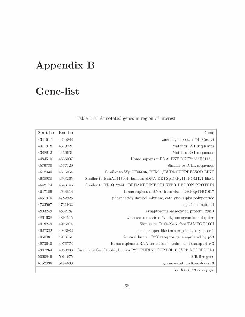
Appendix B

Gene-list

Table B.1: Annotated genes in region of interest

Start bp End bp Gene

4341617 4355088 zinc finger protein 74 (Cos52)

4371978 4379221 Matches EST sequences

4388912 4436631 Matches EST sequences

4484510 4535007 Homo sapiens mRNA; EST DKFZp586E2117r1

4576780 4577120 Similar to IGLL sequences

4612030 4615254 Similar to Wp:CE06096, BEM-1/BUD5 SUPPRESSOR-LIKE

4638988 4643265 Similar to Em:AL117401, humam cDNA DKFZp434P211, POM121-like 1

4642174 4643146 Similar to TR:Q12844 : BREAKPOINT CLUSTER REGION PROTEIN

4647189 4648818 Homo sapiens mRNA; from clone DKFZp434G1017

4651915 4782925 phosphatidylinositol 4-kinase, catalytic, alpha polypeptide

4723507 4731932 heparin cofactor II

4803249 4832187 synaptosomal-associated protein, 29kD

4861638 4894515 avian sarcoma virus (v-crk) oncogene homolog-like

4918249 4925974 Similar to Tr:O42346, frog TAMEGOLOH

4927322 4943982 leucine-zipper-like transcriptional regulator 1

4960081 4973751 A novel human P2X receptor gene regulated by p53

4973640 4976773 Homo sapiens mRNA for cationic amino acid transporter 3

4987264 4989938 Similar to Sw:O15547, human P2X PURINOCEPTOR 6 (ATP RECEPTOR)

5060849 5064675 BCR like gene

5152896 5154638 gamma-glutamyltransferase 3

continued on next page

66

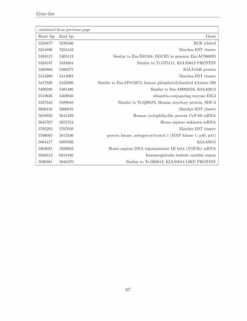
Gene-list

continued from previous page

Start bp End bp Gene

5235677 5239506 BCR related

5254896 5255442 Matches EST cluster

5304515 5305113 Similar to Em:X91348, DGCR5 in genomic Em:AC000095

5333187 5334084 Similar to Tr:O75111, KIAA0612 PROTEIN

5389868 5396377 KIAA1020 protein

5413200 5414994 Matches EST cluster

5417928 5433300 Similar to Em:AF012872, human phosphatidylinositol 4-kinase 230

5490598 5491486 Similar to Em:AB002316, KIAA0612

5512636 5568940 ubiquitin-conjugating enzyme E2L3

5587342 5589048 Similar to Tr:Q99470, Human secretory protein, SDF-2

5606416 5606845 Matches EST cluster

5610928 5641329 Human cyclophilin-like protein CyP-60 mRNA

5645767 5655734 Homo sapiens unknown mRNA

5705295 5707050 Matches EST cluster

5708005 5812536 protein kinase, mitogen-activated 1 (MAP kinase 1; p40, p41)

5864417 5897826 KIAA0015

5902021 5920802 Homo sapiens DNA topoisomerase III beta (TOP3b) mRNA

5930513 6814186 Immunoglobulin lambda variable region

5936381 5940470 Similar to Tr:O60813, KIAA0014 LIKE PROTEIN

67