Predicting Wide Receiver Trajectories in American Football

Namhoon Lee and Kris M. Kitani

The Robotics Institute, Carnegie Mellon University

namhoonl@andrew.cmu.edu, kkitani@cs.cmu.edu

Abstract

Predicting the trajectory of a wide receiver in the game

of American football requires prior knowledge about the

game (e.g., route trees, defensive formations) and an ac-

curate model of how the environment will change over

time (e.g., opponent reaction strategies, motion attributes

of players). Our aim is to build a computational model of

the wide receiver, which takes into account prior knowledge

about the game and short-term predictive models of how the

environment will change over time. While prior knowledge

of the game is readily accessible, it is quite challenging to

build predictive models of how the environment will change

over time. We propose several models for predicting short-

term motions of opponent players to generate dynamic input

features for our wide receiver forecasting model. In par-

ticular, we model the wide receiver with a Markov Deci-

sion Process (MDP), where the reward function is a linear

combination of static features (prior knowledge about the

game) and dynamic features (short-term prediction of oppo-

nent players). Since the dynamic features change over time,

we make recursive calls to an inference procedure over the

MDP while updating the dynamic features. We validate our

technique on a video dataset of American football plays.

Our results show that more informed models that accurately

predict the motions of the defensive players are better at

forecasting wide receiver plays.

1. Introduction

The task of analyzing human activity has received much

attention in the field of computer vision. Among the many

sub-fields dealing with human activities, we address the

problem of activity forecasting which refers to the task of

inferring the future actions of people from visual input [15].

Human activity forecasting is a different task from that of

recognition, detection or tracking. Vision-based activity

forecasting aims to predict how an agent will act in the fu-

ture given a single image of the world.

Forecasting human activity in dynamic environments

is extremely difficult because changes in the environment

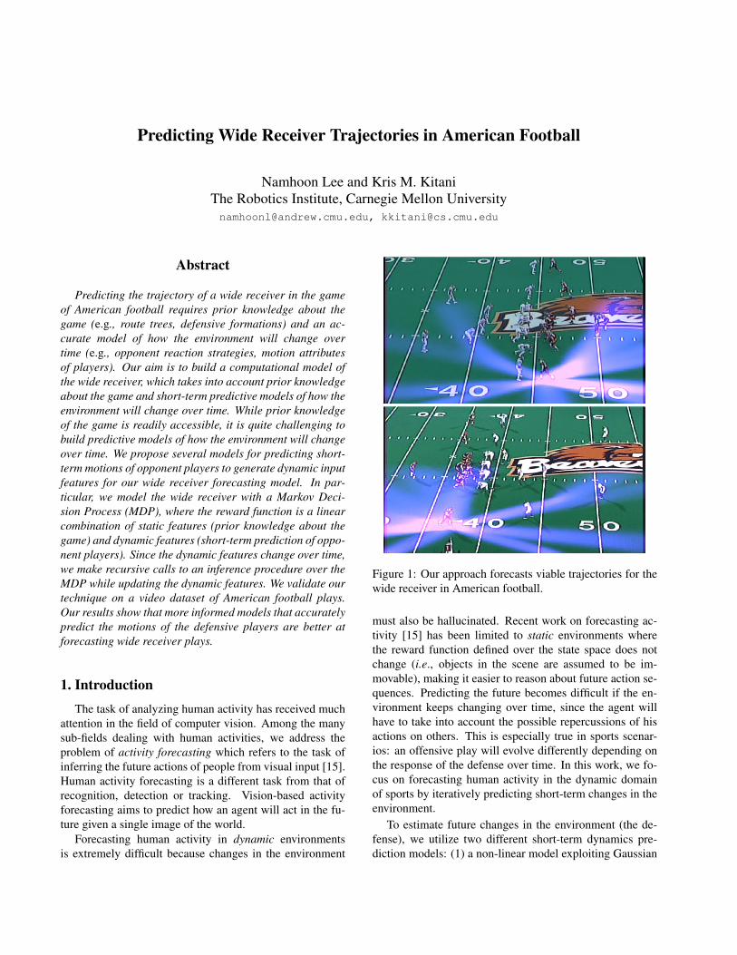
Figure 1: Our approach forecasts viable trajectories for the

wide receiver in American football.

must also be hallucinated. Recent work on forecasting ac-

tivity [15] has been limited to static environments where

the reward function defined over the state space does not

change (i.e., objects in the scene are assumed to be im-

movable), making it easier to reason about future action se-

quences. Predicting the future becomes difficult if the en-

vironment keeps changing over time, since the agent will

have to take into account the possible repercussions of his

actions on others. This is especially true in sports scenar-

ios: an offensive play will evolve differently depending on

the response of the defense over time. In this work, we fo-

cus on forecasting human activity in the dynamic domain

of sports by iteratively predicting short-term changes in the

environment.

To estimate future changes in the environment (the de-

fense), we utilize two different short-term dynamics pre-

diction models: (1) a non-linear model exploiting Gaussian

Trajectories of football playersAmerican football video t

WR

CB

(a) Registration of an American football video

WRCB

WRCB

goal goal

Static Environment Dynamic Environment

(b) Static Environment VS Dynamic Environment

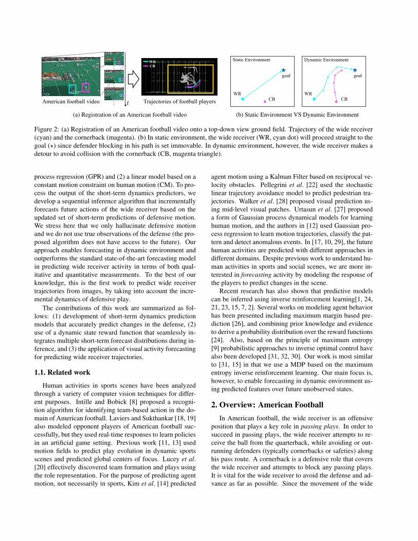
Figure 2: (a) Registration of an American football video onto a top-down view ground field. Trajectory of the wide receiver

(cyan) and the cornerback (magenta). (b) In static environment, the wide receiver (WR, cyan dot) will proceed straight to the

goal (⋆) since defender blocking in his path is set immovable. In dynamic environment, however, the wide receiver makes a

detour to avoid collision with the cornerback (CB, magenta triangle).

process regression (GPR) and (2) a linear model based on a

constant motion constraint on human motion (CM). To pro-

cess the output of the short-term dynamics predictors, we

develop a sequential inference algorithm that incrementally

forecasts future actions of the wide receiver based on the

updated set of short-term predictions of defensive motion.

We stress here that we only hallucinate defensive motion

and we do not use true observations of the defense (the pro-

posed algorithm does not have access to the future). Our

approach enables forecasting in dynamic environment and

outperforms the standard state-of-the-art forecasting model

in predicting wide receiver activity in terms of both qual-

itative and quantitative measurements. To the best of our

knowledge, this is the first work to predict wide receiver

trajectories from images, by taking into account the incre-

mental dynamics of defensive play.

The contributions of this work are summarized as fol-

lows: (1) development of short-term dynamics prediction

models that accurately predict changes in the defense, (2)

use of a dynamic state reward function that seamlessly in-

tegrates multiple short-term forecast distributions during in-

ference, and (3) the application of visual activity forecasting

for predicting wide receiver trajectories.

1.1. Related work

Human activities in sports scenes have been analyzed

through a variety of computer vision techniques for differ-

ent purposes. Intille and Bobick [8] proposed a recogni-

tion algorithm for identifying team-based action in the do-

main of American football. Laviers and Sukthankar [18, 19]

also modeled opponent players of American football suc-

cessfully, but they used real-time responses to learn policies

in an artificial game setting. Previous work [11, 13] used

motion fields to predict play evolution in dynamic sports

scenes and predicted global centers of focus. Lucey et al.

[20] effectively discovered team formation and plays using

the role representation. For the purpose of predicting agent

motion, not necessarily in sports, Kim et al. [14] predicted

agent motion using a Kalman Filter based on reciprocal ve-

locity obstacles. Pellegrini et al. [22] used the stochastic

linear trajectory avoidance model to predict pedestrian tra-

jectories. Walker et al. [28] proposed visual prediction us-

ing mid-level visual patches. Urtasun et al. [27] proposed

a form of Gaussian process dynamical models for learning

human motion, and the authors in [12] used Gaussian pro-

cess regression to learn motion trajectories, classify the pat-

tern and detect anomalous events. In [17, 10, 29], the future

human activities are predicted with different approaches in

different domains. Despite previous work to understand hu-

man activities in sports and social scenes, we are more in-

terested in forecasting activity by modeling the response of

the players to predict changes in the scene.

Recent research has also shown that predictive models

can be inferred using inverse reinforcement learning[1, 24,

21, 23, 15, 7, 2]. Several works on modeling agent behavior

has been presented including maximum margin based pre-

diction [26], and combining prior knowledge and evidence

to derive a probability distribution over the reward functions

[24]. Also, based on the principle of maximum entropy

[9] probabilistic approaches to inverse optimal control have

also been developed [31, 32, 30]. Our work is most similar

to [31, 15] in that we use a MDP based on the maximum

entropy inverse reinforcement learning. Our main focus is,

however, to enable forecasting in dynamic environment us-

ing predicted features over future unobserved states.

2. Overview: American Football

In American football, the wide receiver is an offensive

position that plays a key role in passing plays. In order to

succeed in passing plays, the wide receiver attempts to re-

ceive the ball from the quarterback, while avoiding or out-

running defenders (typically cornerbacks or safeties) along

his pass route. A cornerback is a defensive role that covers

the wide receiver and attempts to block any passing plays.

It is vital for the wide receiver to avoid the defense and ad-

vance as far as possible. Since the movement of the wide

receiver can be different depending on the defenders, pre-

dicting the wide receiver trajectories should take into ac-

count the possible changes to the environment (see Figure

2b). To simplify our problem, we build our proposed pre-

diction model based on an assumption that the cornerback

is the primary defender affecting the wide receiver’s future

activity and contributes to the changes in the environment

(i.e., generates dynamic features). In our scenario, the op-

ponent (CB) forms a negative force field which repells the

wide receiver.

We describe how dynamics of the environment is pre-

dicted in Section 3. Then, using the proposed methods to

predict the dynamic features (i.e., defensive motion) we per-

form sequential inference for predicting wide receiver tra-

jectories in Section 4. We present our comprehensive ex-

perimental results in Section 5 along with an application to

sports analytics in Section 6.

3. Prediction of the Dynamic Environment

3.1. Non­linear feature regressor

One approach of predicting opponent reaction is to use

a regressor trained in a supervised manner. Instead of as-

suming a simple parametric model which lacks expressive

power, we propose to use a finer approach, Gaussian pro-

cess regression (GPR), which gives more flexibility in rep-

resenting data [25] as well as variance estimates that we

use for generating dynamic features. Fully specified by its

mean function m(x) and covariance function k(x, x′), the

Gaussian process generates distribution over functions f as

follows,

f ∼ GP(m(x), k(x, x′)) (1)

where we used linear model for the mean function m(x) =wx + b, and an isotropic Gaussian with noise for the co-

variance function k(x, x′) = σ2yexp(−

(x−x′)2

2l2 ) + σ2nδii′ .

The hyperparameters {a, b, σy, σn, l} are obtained by a gra-

dient based numerical optimization routine. Given some

noisy observations, Gaussian process regression not only

fits the training examples but also computes the posterior

that yields predictions for unseen test cases,

y∗|y ∼ N (µ∗ +ΣT

∗Σ−1(y− µ),Σ∗∗ − ΣT

∗Σ−1Σ∗) (2)

where µ and µ∗ is the training mean and the test mean re-

spectively, and Σ is training set covariance, Σ∗ is training-

test set covariance and Σ∗∗ is test set covariance. For the

known function values of the training cases y, the predic-

tion y∗ corresponding to the test inputs x∗ is the predicted

position of the cornerback in our case.

Given the GPR model, we collect the training samples

x(i) and labels y(i) as follows. We constructed x of train-

ing examples firstly by concatenating all the relative dis-

tance vectors pointing from the centroid c0 of the trajec-

tory pair to the control points ci that are uniformly picked

centroid

WR

CB

control points

Transformation Normalization

opponent

reactionlt+1

lt+2

lt+k Training

examples

L

~c1~c2

~cn

C

ci

c0

y

x

{(x(i), y(i))}

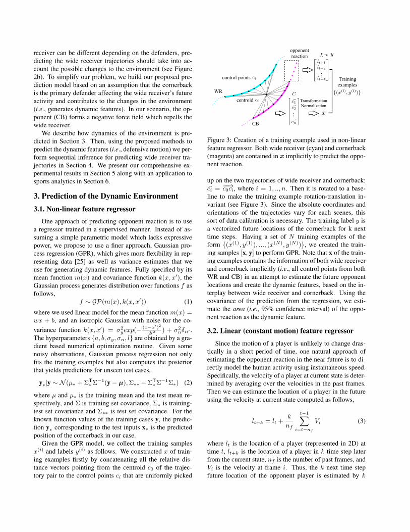
Figure 3: Creation of a training example used in non-linear

feature regressor. Both wide receiver (cyan) and cornerback

(magenta) are contained in x implicitly to predict the oppo-

nent reaction.

up on the two trajectories of wide receiver and cornerback:

~ci = −−→c0ci, where i = 1, .., n. Then it is rotated to a base-

line to make the training example rotation-translation in-

variant (see Figure 3). Since the absolute coordinates and

orientations of the trajectories vary for each scenes, this

sort of data calibration is necessary. The training label y is

a vectorized future locations of the cornerback for k next

time steps. Having a set of N training examples of the

form {(x(1), y(1)), ..., (x(N), y(N))}, we created the train-

ing samples [x, y] to perform GPR. Note that x of the train-

ing examples contains the information of both wide receiver

and cornerback implicitly (i.e., all control points from both

WR and CB) in an attempt to estimate the future opponent

locations and create the dynamic features, based on the in-

terplay between wide receiver and cornerback. Using the

covariance of the prediction from the regression, we esti-

mate the area (i.e., 95% confidence interval) of the oppo-

nent reaction as the dynamic feature.

3.2. Linear (constant motion) feature regressor

Since the motion of a player is unlikely to change dras-

tically in a short period of time, one natural approach of

estimating the opponent reaction in the near future is to di-

rectly model the human activity using instantaneous speed.

Specifically, the velocity of a player at current state is deter-

mined by averaging over the velocities in the past frames.

Then we can estimate the location of a player in the future

using the velocity at current state computed as follows,

lt+k = lt +k

nf

t−1∑

i=t−nf

Vi (3)

where lt is the location of a player (represented in 2D) at

time t, lt+k is the location of a player in k time step later

from the current state, nf is the number of past frames, and

Vi is the velocity at frame i. Thus, the k next time step

future location of the opponent player is estimated by k

multiple of the average velocity per frame plus the current

location. Depending on the number past frames used, the

average velocity will be different as well as the estimated

locations of a player. The estimated locations of a player

is then Gaussian filtered to form the area of the opponent

reaction as the dynamic feature.

4. Forecasting in Dynamic Environments

4.1. Maximum entropy inverse optimal control

A Markov decision process (MDP) is a mathematical

model for decision making process [3, 6] in a form of

Markov chains defined with state s, action a, transition

probability ps′

s,a and initial distribution p(s0). As a stochas-

tic process, an agent takes an action to move to another state

with the transition probability and accordingly takes reward

r(s) for that action. In our problem domain, the location of

an agent (i.e., wide receiver) from a top-down view in world

coordinate represents the state s = [x, y] and the movement

to an adjacent state near the current state is defined as action

a for the agent. The goal of MDP is to find a policy π for the

agent, which maximizes the function of cumulative rewards

for a sequence of actions. The reward of a path R(ζ) is the

sum of all state rewards r(s) which is the sum of weighted

feature responses F(s) ∈ ℜk along the path,

R(ζ;θ) =∑

s∈ζ

r(s;θ) =∑

s∈ζ

θ ·F(s) (4)

where the path ζ is a sequence of states, θ is a vector of

reward weights, and the reward of a state r(s;θ) represents

the immediate reward received at a state s. The feature re-

sponses F(s) =[

F1(s),F2(s), ...,Fk(s)]

are a series of

different types of features where each feature response is

represented as a 2D feature response map over the football

field. In this work, we not only model static features, but

also dynamic features to represent the high cost (e.g., low

reward) region which is attributed to the opponent reaction

that changes over time.

As the reward weights θ is typically unknown, in in-

verse reinforcement learning (IRL) or inverse optimal con-

trol (IOC) it is attempted to recover the reward weights from

demonstrated examples such that the agent model generates

action sequences similar to a set of demonstrated examples

[1]. In maximum entropy inverse reinforcement learning

[31], the distribution over a path ζ is defined as,

p(ζ;θ) =eR(ζ;θ)

Z(θ)=

e∑

s∈ζ θ·F(s)

Z(θ)(5)

where Z(θ) is the normalizing partition function, showing

that a path with higher rewards is exponentially more pre-

ferred. With the objective of recovering the optimal reward

function parameters θ∗, we perform an exponentiated gra-

dient descent to maximize the likelihood of the maximum

entropy of the observed data,

θ∗ = argmaxθ L(θ) = argmaxθ

∑

ζ

log p(ζ;θ) (6)

whereL(θ) is the log-likelihood of the observation which is

the trajectory of the wide receiver in our case. The gradient

of the log-likelihood is expressed by the difference between

the empirical mean feature counts f, which is the sum of the

feature counts over all demonstrated trajectories ζ and the

expected mean feature counts fθ over the sampled trajec-

tories ζ from forecast distribution, which is represented by

state visitation frequency D(s) as follows,

f =∑

ζ

∑

s∈ζ

F(s),

fθ =∑

ζ

p(ζs;θ)∑

s∈ζ

F(s) =∑

s

D(s)F(s).(7)

As the expected feature count matches to the empirical fea-

ture count, the learner aims to mimic the demonstrated be-

havior [1].

4.2. Sequential inference in dynamic environment

In dynamic environment where dynamic features come

from the opponent reaction, the state reward should change

over time as players move during the play. We thus define

the state reward as a linear combination of the static state

reward and the dynamic state reward as the following,

rt(s;θ) = r(s;θs) + rt(s;θd) (8)

where rt(s;θ) represents the time-varying state reward at

time t while θs and θd are the reward weights of the static

features and the dynamic features respectively.

Unlike the standard forecasting approaches in static en-

vironments where they performed a single long-term fore-

casting [15], we perform multiple short-term predictions se-

quentially while updating the dynamic feature. Note in this

process that we do not use any real-time observations to es-

timate the dynamic features. It is our interest to perform a

long sequenced short-term forecasts based on the predicted

dynamic features.

To be more precise, the forecast distribution is expressed

as a state visitation frequency D(s) which is computed by

propagating the initial distribution D(s0) using optimal pol-

icy. In our case we have a short-term forecast distribution

D(t)(s) at each time step t, which changes over time and

gradually produces the final forecast distribution. In this

process, we pass the previous short-term forecast distribu-

tion as input to the next inference cycle so that the fore-

casting proceeds without discontinuity. It is also necessary

to have the predicted short-term trajectories of the wide re-

ceiver and cornerback, ζWR and ζCB respectively, for the

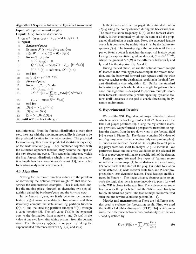
Algorithm 1 Sequential Inference in Dynamic Environment

Input: θ∗ (optimal reward weight)

Ouput: D(s): forecast distribution

1: ζWR ← ζWR, ζCB ← ζCB , and D(s0)← 12: repeat

3: Backward pass:

4: Estimate Ft(s) with ζWR and ζCB

5: rt(s;θ∗) = r(s;θ∗

s) + θ∗d · Ft(s)

6: for n=N,...,2,1 do

7: V (n)(sgoal)← 08: Q(n)(s, a) = rt(s;θ

∗) + Eps′s,a

[V (n)(s′)]

9: V (n−1)(s) = soft maxa Q(n)(s, a)10: end for

11: πθ(a|s)← eQ(s,a)−V (s)

12: Forward pass:

13: for n = 1, 2, ..., Ns do

14: D(n)(sgoal)← 015: D(n+1)(s) =

∑

s′,a

pss′,aπθ(a|s′)D(n)(s′)

16: ζWR ← max(D(n+1)(s))17: end for

18: D(s) =∑

n D(n)(s)

19: D(s0)← D(s)

20: fθ =∑

s F(s)D(s)21: until WR reaches to the goal

next inference. From the forecast distribution at each time

step, the state with the maximum probability is chosen to be

the predicted location for the wide receiver. The predicted

locations altogether form the predicted short-term trajectory

of the wide receiver ζWR. Then combined together with

the estimated opponent location, they become the input of

the next forecasting cycle. This sequential inference yields

the final forecast distribution which is no shorter in predic-

tion length than the current state-of-the-art [15], but enables

forecasting in dynamic environment.

4.3. Algorithm

Solving for the reward function reduces to the problem

of recovering the optimal reward weight θ∗ that best de-

scribes the demonstrated examples. This is achieved dur-

ing the training phase, through an alternating two-step al-

gorithm called the backward pass and the forward pass.

In the backward pass, we firstly generate the dynamic

feature Ft(s) using ground-truth observations, and then

iteratively compute the state-action log partition function

Q(s, a) and the state log partition function V (s) through

a value iteration [3]. The soft value V (s) is the expected

cost to the destination from a state s, and Q(s, a) is the

value at one step later after taking action a from the current

state. Then the policy πθ(a|s) is computed by taking the

exponentiated difference between Q(s, a) and V (s).

In the forward pass, we propagate the initial distribution

D(s0) using the policy obtained during the backward pass.

The state visitation frequency D(s), or the forecast distri-

bution, is then computed by taking the sum of all the prop-

agated distribution at each step. Next, the expected feature

count fθ is computed by multiplying D(s) by the feature re-

sponses f(s). The two-step algorithm repeats until the ex-

pected feature count fθ matches the empirical feature count

f using the exponentiated gradient descent, θ ← θeλ∇L(θ),

where the gradient ∇L(θ) is the difference between fθ and

fθ, and λ is the step size (Eq. 6 and 7).

During the test phase, we use the optimal reward weight

θ∗ learned in the training phase to compute the reward func-

tion, and the backward-forward pair repeats until the wide

receiver reaches to the destination resulting in the final fore-

cast distribution (see Algorithm 1). Unlike the standard

forecasting approach which takes a single long-term infer-

ence, our algorithm is designed to perform multiple short-

term forecasts incrementally while updating dynamic fea-

tures until it reaches to the goal to enable forecasting in dy-

namic environment.

5. Experimental Results

We used the OSU Digital Scout Project’s football dataset

which includes the tracking results of all 22 players with the

labels of player positions [5]. Using the registration matri-

ces provided, we performed a perspective transform to reg-

ister the players from the top-down view in the football field

[4] as seen in Figure 2a. The dataset contains 20 videos of

passing plays (each video contains only one passing play).

10 videos are selected based on its lengths (several pass-

ing plays were too short to analyze, e.g., 2 seconds). We

performed leave-one-out cross-validation on the selected 10

videos to prevent overfitting to a specific split of the dataset.

Feature maps: We used five types of features repre-

sented as a feature map: (1) linear distance to the end zone,

(2) cornerback at the start of the play, (3) initial formation

of the defense, (4) wide receiver route tree, and (5) our pro-

posed short-term dynamics feature. These features are illus-

trated in Figure 4. The linear distance features aims to en-

code the logic that there is more incentive to press forward

as the WR is closer to the goal line. The wide receiver route

tree encodes the prior belief that the WR is more likely to

follow standardized paths. The feature maps are normalized

such that the reward values range from [0,−1].Metrics and measurements: There are 4 different met-

rics used to evaluate the forecasting result. First, we used

the Kullback-Leibler divergence (KLD) [16] which mea-

sures the difference between two probability distributions

P and Q defined by

DKL(P ||Q) =∑

i

P (i)P (i)

Q(i)(9)

(a) Linear distance (b) Cornerback

(c) Defense (d) Route tree

(e) Dynamic feature (f) Reward map

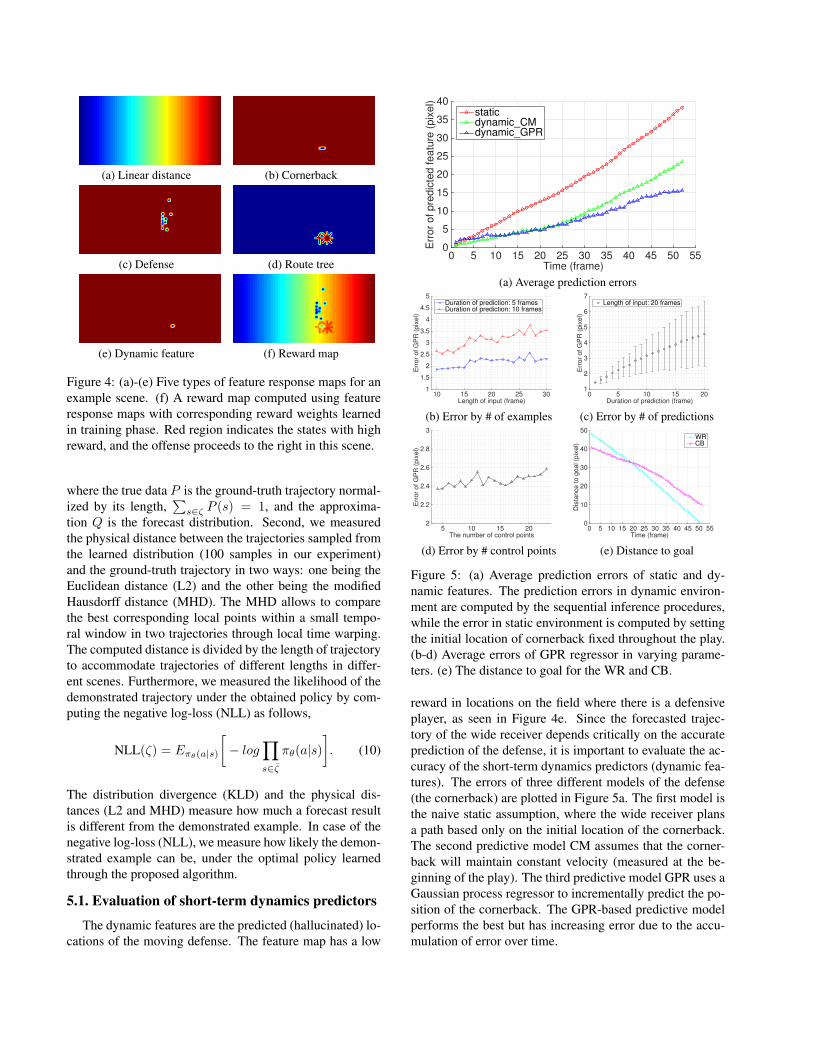
Figure 4: (a)-(e) Five types of feature response maps for an

example scene. (f) A reward map computed using feature

response maps with corresponding reward weights learned

in training phase. Red region indicates the states with high

reward, and the offense proceeds to the right in this scene.

where the true data P is the ground-truth trajectory normal-

ized by its length,∑

s∈ζ P (s) = 1, and the approxima-

tion Q is the forecast distribution. Second, we measured

the physical distance between the trajectories sampled from

the learned distribution (100 samples in our experiment)

and the ground-truth trajectory in two ways: one being the

Euclidean distance (L2) and the other being the modified

Hausdorff distance (MHD). The MHD allows to compare

the best corresponding local points within a small tempo-

ral window in two trajectories through local time warping.

The computed distance is divided by the length of trajectory

to accommodate trajectories of different lengths in differ-

ent scenes. Furthermore, we measured the likelihood of the

demonstrated trajectory under the obtained policy by com-

puting the negative log-loss (NLL) as follows,

NLL(ζ) = Eπθ(a|s)

[

− log∏

s∈ζ

πθ(a|s)

]

. (10)

The distribution divergence (KLD) and the physical dis-

tances (L2 and MHD) measure how much a forecast result

is different from the demonstrated example. In case of the

negative log-loss (NLL), we measure how likely the demon-

strated example can be, under the optimal policy learned

through the proposed algorithm.

5.1. Evaluation of short­term dynamics predictors

The dynamic features are the predicted (hallucinated) lo-

cations of the moving defense. The feature map has a low

Time (frame)0 5 10 15 20 25 30 35 40 45 50 55

Err

or

of pre

dic

ted featu

re (

pix

el)

0

5

10

15

20

25

30

35

40staticdynamic_CMdynamic_GPR

(a) Average prediction errors

Length of input (frame)10 15 20 25 30

Err

or

of G

PR

(pix

el)

1

1.5

2

2.5

3

3.5

4

4.5

5Duration of prediction: 5 framesDuration of prediction: 10 frames

(b) Error by # of examples

Duration of prediction (frame)0 5 10 15 20

Err

or

of G

PR

(pix

el)

1

2

3

4

5

6

7Length of input: 20 frames

(c) Error by # of predictions

The number of control points5 10 15 20

Err

or

of G

PR

(pix

el)

2

2.2

2.4

2.6

2.8

3

(d) Error by # control points

Time (frame)0 5 10 15 20 25 30 35 40 45 50 55

Dis

tance to g

oal (p

ixel)

0

10

20

30

40

50WRCB

(e) Distance to goal

Figure 5: (a) Average prediction errors of static and dy-

namic features. The prediction errors in dynamic environ-

ment are computed by the sequential inference procedures,

while the error in static environment is computed by setting

the initial location of cornerback fixed throughout the play.

(b-d) Average errors of GPR regressor in varying parame-

ters. (e) The distance to goal for the WR and CB.

reward in locations on the field where there is a defensive

player, as seen in Figure 4e. Since the forecasted trajec-

tory of the wide receiver depends critically on the accurate

prediction of the defense, it is important to evaluate the ac-

curacy of the short-term dynamics predictors (dynamic fea-

tures). The errors of three different models of the defense

(the cornerback) are plotted in Figure 5a. The first model is

the naive static assumption, where the wide receiver plans

a path based only on the initial location of the cornerback.

The second predictive model CM assumes that the corner-

back will maintain constant velocity (measured at the be-

ginning of the play). The third predictive model GPR uses a

Gaussian process regressor to incrementally predict the po-

sition of the cornerback. The GPR-based predictive model

performs the best but has increasing error due to the accu-

mulation of error over time.

PL

AY

1P

LA

Y2

PL

AY

3

(a) Regular (b) CM (c) GPR

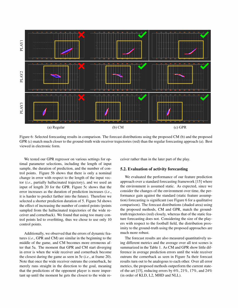
Figure 6: Selected forecasting results in comparison. The forecast distributions using the proposed CM (b) and the proposed

GPR (c) match much closer to the ground-truth wide receiver trajectories (red) than the regular forecasting approach (a). Best

viewed in electronic form.

We tested our GPR regressor on various settings for op-

timal parameter selections, including the length of input

sample, the duration of prediction, and the number of con-

trol points. Figure 5b shows that there is only a nominal

change in error with respect to the length of the input vec-

tor (i.e., partially hallucinated trajectory), and we used an

input of length 20 for the GPR. Figure 5c shows that the

error increases as the duration of prediction increases (i.e.,

it is harder to predict farther into the future). Therefore we

selected a shorter prediction duration of 5. Figure 5d shows

the effect of increasing the number of control points (points

sampled from the hallucinated trajectories of the wide re-

ceiver and cornerback). We found that using too many con-

trol points led to overfitting, thus we chose to use only 10

control points.

Additionally, we observed that the errors of dynamic fea-

tures (i.e., GPR and CM) are similar in the beginning to the

middle of the game, and CM becomes more erroneous af-

ter that 5a. The moment that GPR and CM start diverging

in error is when the wide receiver and cornerback become

the closest during the game as seen in 5e (i.e., at frame 20).

Note that once the wide receiver outruns the cornerback, he

merely runs straight in the direction to the goal, meaning

that the predictions of the opponent player is more impor-

tant up until the moment he gets the closest to the wide re-

ceiver rather than in the later part of the play.

5.2. Evaluation of activity forecasting

We evaluated the performance of our feature prediction

approach over a standard forecasting framework [15] where

the environment is assumed static. As expected, since we

consider the changes of the environment over time, the per-

formance gain against the standard (static feature assump-

tion) forecasting is significant (see Figure 6 for a qualitative

comparison). The forecast distributions (shaded area) using

the proposed methods, CM and GPR, match the ground-

truth trajectories (red) closely, whereas that of the static fea-

ture forecasting does not. Considering the size of the play-

ers with respect to the football field, the distribution prox-

imity to the ground-truth using the proposed approaches are

much more robust.

The forecast results are also measured quantitatively us-

ing different metrics and the average over all test scenes is

summarized in the Table 1. As CM and GPR show little dif-

ference in average prediction errors until the wide receiver

outruns the cornerback as seen in Figure 5a their forecast

results turn out to be analogous to each other. Over all error

metrics, the proposed methods outperform the current state-

of-the-art [15], reducing errors by 6%, 21%, 17%, and 24%

(in order of KLD, L2, MHD and NLL).

t = 0 t = 10 t = 20 t = 30 t = 40

t = 50 t = 60 t = 70 t = 80 t = 90

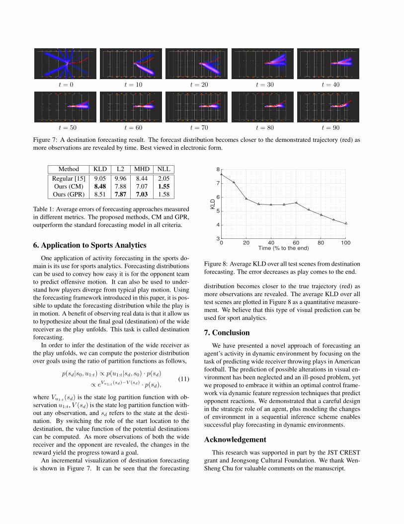
Figure 7: A destination forecasting result. The forecast distribution becomes closer to the demonstrated trajectory (red) as

more observations are revealed by time. Best viewed in electronic form.

Method KLD L2 MHD NLL

Regular [15] 9.05 9.96 8.44 2.05

Ours (CM) 8.48 7.88 7.07 1.55

Ours (GPR) 8.51 7.87 7.03 1.58

Table 1: Average errors of forecasting approaches measured

in different metrics. The proposed methods, CM and GPR,

outperform the standard forecasting model in all criteria.

6. Application to Sports Analytics

One application of activity forecasting in the sports do-

main is its use for sports analytics. Forecasting distributions

can be used to convey how easy it is for the opponent team

to predict offensive motion. It can also be used to under-

stand how players diverge from typical play motion. Using

the forecasting framework introduced in this paper, it is pos-

sible to update the forecasting distribution while the play is

in motion. A benefit of observing real data is that it allow us

to hypothesize about the final goal (destination) of the wide

receiver as the play unfolds. This task is called destination

forecasting.

In order to infer the destination of the wide receiver as

the play unfolds, we can compute the posterior distribution

over goals using the ratio of partition functions as follows,

p(sd|s0, u1:t) ∝ p(u1:t|sd, s0) · p(sd)

∝ eVu1:t(sd)−V (sd) · p(sd),

(11)

where Vu1:t(sd) is the state log partition function with ob-

servation u1:t, V (sd) is the state log partition function with-

out any observation, and sd refers to the state at the desti-

nation. By switching the role of the start location to the

destination, the value function of the potential destinations

can be computed. As more observations of both the wide

receiver and the opponent are revealed, the changes in the

reward yield the progress toward a goal.

An incremental visualization of destination forecasting

is shown in Figure 7. It can be seen that the forecasting

Time (% to the end)0 20 40 60 80 100

KLD

3

4

5

6

7

8

Figure 8: Average KLD over all test scenes from destination

forecasting. The error decreases as play comes to the end.

distribution becomes closer to the true trajectory (red) as

more observations are revealed. The average KLD over all

test scenes are plotted in Figure 8 as a quantitative measure-

ment. We believe that this type of visual prediction can be

used for sport analytics.

7. Conclusion

We have presented a novel approach of forecasting an

agent’s activity in dynamic environment by focusing on the

task of predicting wide receiver throwing plays in American

football. The prediction of possible alterations in visual en-

vironment has been neglected and an ill-posed problem, yet

we proposed to embrace it within an optimal control frame-

work via dynamic feature regression techniques that predict

opponent reactions. We demonstrated that a careful design

in the strategic role of an agent, plus modeling the changes

of environment in a sequential inference scheme enables

successful play forecasting in dynamic environments.

Acknowledgement

This research was supported in part by the JST CREST

grant and Jeongsong Cultural Foundation. We thank Wen-

Sheng Chu for valuable comments on the manuscript.

References

[1] P. Abbeel and A. Y. Ng. Apprenticeship learning via inverse

reinforcement learning. In Proceedings of the twenty-first in-

ternational conference on Machine learning, page 1. ACM,

2004.

[2] C. L. Baker, R. Saxe, and J. B. Tenenbaum. Action under-

standing as inverse planning. Cognition, 113(3):329–349,

2009.

[3] R. Bellman. Dynamic programming and lagrange multipli-

ers. Proceedings of the National Academy of Sciences of the

United States of America, 42(10):767, 1956.

[4] R. Hess and A. Fern. Improved video registration using non-

distinctive local image features. In Computer Vision and

Pattern Recognition, 2007. CVPR’07. IEEE Conference on,

pages 1–8. IEEE, 2007.

[5] R. Hess and A. Fern. Discriminatively trained particle filters

for complex multi-object tracking. In Computer Vision and

Pattern Recognition, 2009. CVPR 2009. IEEE Conference

on, pages 240–247. IEEE, 2009.

[6] R. A. Howard. Dynamic programming and markov pro-

cesses.. 1960.

[7] D.-A. Huang and K. M. Kitani. Action-reaction: Forecasting

the dynamics of human interaction. In Computer Vision–

ECCV 2014, pages 489–504. Springer, 2014.

[8] S. S. Intille and A. F. Bobick. Recognizing planned, multi-

person action. Computer Vision and Image Understanding,

81(3):414–445, 2001.

[9] E. T. Jaynes. Information theory and statistical mechanics.

Physical review, 106(4):620, 1957.

[10] Y. Jiang and A. Saxena. Modeling high-dimensional humans

for activity anticipation using gaussian process latent crfs. In

Robotics: Science and Systems, RSS, 2014.

[11] K. Kim, M. Grundmann, A. Shamir, I. Matthews, J. Hod-

gins, and I. Essa. Motion fields to predict play evolution

in dynamic sport scenes. In Computer Vision and Pattern

Recognition (CVPR), 2010 IEEE Conference on, pages 840–

847. IEEE, 2010.

[12] K. Kim, D. Lee, and I. Essa. Gaussian process regression

flow for analysis of motion trajectories. In Computer Vi-

sion (ICCV), 2011 IEEE International Conference on, pages

1164–1171. IEEE, 2011.

[13] K. Kim, D. Lee, and I. Essa. Detecting regions of interest

in dynamic scenes with camera motions. In Computer Vision

and Pattern Recognition (CVPR), 2012 IEEE Conference on,

pages 1258–1265. IEEE, 2012.

[14] S. Kim, S. J. Guy, W. Liu, R. W. Lau, M. C. Lin,

and D. Manocha. Predicting pedestrian trajectories using

velocity-space reasoning. In Algorithmic Foundations of

Robotics X, pages 609–623. Springer, 2013.

[15] K. M. Kitani, B. D. Ziebart, J. A. D. Bagnell, and M. Hebert.

Activity forecasting. In European Conference on Computer

Vision. Springer, October 2012.

[16] S. Kullback and R. A. Leibler. On information and suffi-

ciency. The annals of mathematical statistics, pages 79–86,

1951.

[17] T. Lan, T.-C. Chen, and S. Savarese. A hierarchical repre-

sentation for future action prediction. In Computer Vision–

ECCV 2014, pages 689–704. Springer, 2014.

[18] K. Laviers and G. Sukthankar. A real-time opponent mod-

eling system for rush football. In IJCAI Proceedings-

International Joint Conference on Artificial Intelligence, vol-

ume 22, page 2476. Citeseer, 2011.

[19] K. R. Laviersa and G. Sukthankarb. Using opponent model-

ing to adapt team play in american football. 2014.

[20] P. Lucey, A. Bialkowski, P. Carr, S. Morgan, I. Matthews,

and Y. Sheikh. Representing and discovering adversarial

team behaviors using player roles. In Computer Vision

and Pattern Recognition (CVPR), 2013 IEEE Conference on,

pages 2706–2713. IEEE, 2013.

[21] G. Neu and C. Szepesvari. Apprenticeship learning using

inverse reinforcement learning and gradient methods. arXiv

preprint arXiv:1206.5264, 2012.

[22] S. Pellegrini, A. Ess, and L. Van Gool. Predicting pedestrian

trajectories. In Visual Analysis of Humans, pages 473–491.

Springer, 2011.

[23] S. Petti and T. Fraichard. Safe motion planning in dy-

namic environments. In Intelligent Robots and Systems,

2005.(IROS 2005). 2005 IEEE/RSJ International Conference

on, pages 2210–2215. IEEE, 2005.

[24] D. Ramachandran and E. Amir. Bayesian inverse reinforce-

ment learning. Urbana, 51:61801.

[25] C. E. Rasmussen. Gaussian processes for machine learning.

2006.

[26] N. D. Ratliff, J. A. Bagnell, and M. A. Zinkevich. Max-

imum margin planning. In Proceedings of the 23rd inter-

national conference on Machine learning, pages 729–736.

ACM, 2006.

[27] R. Urtasun, D. J. Fleet, and P. Fua. 3d people tracking with

gaussian process dynamical models. In Computer Vision and

Pattern Recognition, 2006 IEEE Computer Society Confer-

ence on, volume 1, pages 238–245. IEEE, 2006.

[28] J. Walker, A. Gupta, and M. Hebert. Patch to the future: Un-

supervised visual prediction. In Computer Vision and Pat-

tern Recognition (CVPR), 2014 IEEE Conference on, pages

3302–3309. IEEE, 2014.

[29] D. Xie, S. Todorovic, and S.-C. Zhu. Inferring” dark matter”

and” dark energy” from videos. In Computer Vision (ICCV),

2013 IEEE International Conference on, pages 2224–2231.

IEEE, 2013.

[30] B. D. Ziebart, J. A. Bagnell, and A. K. Dey. The prin-

ciple of maximum causal entropy for estimating interact-

ing processes. Information Theory, IEEE Transactions on,

59(4):1966–1980, 2013.

[31] B. D. Ziebart, A. Maas, J. A. D. Bagnell, and A. Dey. Maxi-

mum entropy inverse reinforcement learning. In Proceeding

of AAAI 2008, July 2008.

[32] B. D. Ziebart, N. Ratliff, G. Gallagher, C. Mertz, K. Pe-

terson, J. A. Bagnell, M. Hebert, A. K. Dey, and S. Srini-

vasa. Planning-based prediction for pedestrians. In Intelli-

gent Robots and Systems, 2009. IROS 2009. IEEE/RSJ Inter-

national Conference on, pages 3931–3936. IEEE, 2009.