PREDICTING WATER CONSTRAINTS TO

PREDICTING WATER CONSTRAINTS TO

PRODUCTIVITY OF CORN

USING PLANT-ENVIRONMENTAL SIMULATION MODELS

A Dissertation

Presented to the Faculty of the Graduate School

of Cornell University

In Partial Fulfillment of the Requirements for the Degree of

Doctor of Philosophy

by

Imo Werner Buttler

January 1989

ACKNOWLEDGEMENTS

I would like to express my sincere appreciation to the

many people who have contributed to this research. It was

a privilege and a real pleasure to have worked under the

direction of Dr. Susan J. Riha. Her enthusiasm for

science and sincere commitment to teaching and learning

were a great source of inspiration for me. I am grateful

to Drs. Dave Pimentel, Gary w. Fick, and R. Jeff Wagenet

for serving as members of my Special Committee and for

providing support and encouragement throughout the course

of my studies at Cornell.

My appreciation is also expressed to Dr. John L.

Hutson, who provided invaluable advice at numerous

occasions and with whom I could always share the highs and

lows of modeling work. I wish to thank Dr. Armand van

Wambeke for giving me the opportunity to serve as a

teaching assistant in his course.

I am very thankful for the friendship and help

received from my fellow graduate students, whose support

was very much appreciated during the last couple of months

of writing the dissertation.

While conducting the field experiment in Brazil,

excellent support was provided by the CPAC scientists and

staff, to whom I will always be very grateful. Allert R.

Suhet and Dr. Elias de Freitas provided invaluable support

V

as collaborators on the project. Dr. Eric Stoner provided

help whenever needed and was an excellent interpreter of

Brazilian culture.

I feel very fortunate to have enjoyed the friendship

and collaboration of Gustavo c. Rodrigues, who became

interested in the experiment and opened up additional

dimensions to the research by conducting a large plant

sampling effort. Many other researchers at the CPAC

contributed greatly through discussions and support in

various form.

The experiment would have been impossible without the

experienced support of Carlao and the hard work of the

TropSoils field team under the direction of Afonso

Rodrigues Boaventura. I want to thank Jose Amauri de

Carvalho 'Zecao' for help in the field, Emival de Matos

Pereira 'Pesquisa' for help with nitrogen analyses, Jatoba

for support with the irrigation system, and the staff of

the meteorological station under the direction of Balbino

for their help with data collection and processing.

I am grateful to Oner Bicakci, who played an

instrumental role in designing the user interface of GAPS,

particularily the screen menus. James Altucher helped

trouble-shoot later version of the program and developed

much of the current version of the plotter.

This project was primarily funded by subgrant SM-CRSP-

012 of the TropSoils program funded by USAID.

vi

TABLE OF CONTENTS

BIOGRAPHICAL SKETCH.

DEDICATION.

ACKNOWLEDGEMENTS .

TABLE OF CONTENTS.

LIST OF TABLES

LIST OF FIGURES

I. INTRODUCTION

References .

. iii

iv

V

. vii

X

xi

1

4

II. GENERAL PURPOSE SIMULATION MODEL OF WATER FLOW IN THE SOIL-PLANT-ATMOSPHERE SYSTEM. 5

2.1

2.2

2.3

2.4

2.5

2.6

Introduction.

Approach.

Program Structure.

Applications.

Future Development.

Software and Hardware Requirements

References.

5

6

8

14

16

17

18

III. WATER FLUXES IN ACID SAVANNA SOILS: A COMPARISON OF APPROACHES. 19

3.1 Introduction.

3.2 Materials and Methods.

3.2.1 Line Source Irrigation Experiment.

3.2.2 Soil and Plant Sampling.

vii

19

24

24

27

3.2.3 Simulation Procedures.

3.2.4 Simulation Input Data.

3.2.4.1 Climate and Location Data . 3.2.4.2 Soil Parameter Estimation . 3.2.4.3 Plant Input Data . 3.2.5 Statistical Analysis . 3.3 Results and Discussion

3.3.1 Water Content Distribution in the Soil Profile over Time under Various Irrigation

28

30

30

31

36

40

42

Treatments 42

3.3.1.1 Fallow Treatments. 43 3.3.1.2 Cropped Treatments 43

3.3.2 Comparison of Predicted and Measured Soil water Contents and Potentials. 48

3.3.2.1 Fallow Treatments. 3.3.2.2 Cropped Treatments

3.3.3 Water Budget Components.

3.3.3.l Fallow Treatments. 3.3.3.2 Cropped Treatments

3.4 Summary and Conclusions.

References.

IV. PREDICTING CORN GROWTH AND YIELDS UNDER VARIABLE

48 56

71

71 76

85

88

WATER INPUTS 92

4.1 Introduction. 92

4.2 Materials and Methods. 94

4.3 Simulation of Crop Growth 95

4.4 Results and Discussion 99

4.4.1 Effect of amount of irrigation water on dry matter accumulation and leaf area development. 99

4.4.1.1 Sequential Harvests. 99

viii

4.4.1.2 Final Harvest. . 101

4.4.2 Comparison of measured and predicted crop growth and development . 105

4.4.3 Simulations of the dynamics of water stress 112

4.5 summary and Conclusions.

References .

. 126

• 128

v. SUMMARY AND CONCLUSIONS. . 130

Appendix A Gaps User's Manual . . 136

ix

LIST OF TABLES

TABLE 2.1 Example of GAPS Summary information table. 15

TABLE 3.1 Soil physical parameters (mean, standard deviation, maximum and minimum values for 50 soil cores from 9 depths (0.07 - 1.85 m) .. 33

TABLE 3.2 Soil input data.

TABLE 3.3 Plant input data ..

39

41

TABLE 4.1 Differences in processes modeled and parameter values between this simulation and the implementation of Stockle and Campbell (1985) . . . . . . . . . . . . 98

TABLE 4.2 Simulated effects of limiting potential maximum rooting depth (0.38 m, 0.53 m, 0.75 m, and 1.05 m) on actual (mm/day) /potential transpiration (mm/day) (TR), deep drainage (mm) (DR) and final above-ground dry matter (kg m-2) (Y) under different irrigation water treatments.125

TABLE 4.3 Harvest index estimated from experimental data (Him), and predicted (HIP) from accumulated stress during pollination (SIP) •..... 126

X

Figure 2.1

Figure 2.2

Figure 2.3

Figure 2.4

Figure 3.1

LIST OF FIGURES

GAPS structure ..... . 9

Currently included simulator modules .... 10

Example of Dependency Diagram (Priestley_Taylor_ETP procedure)

GAPS Screen Menu Format ...•••

12

13

Total amounts of irrigation water received for soil and plant sampling location. a) as a function of distance from the line source b) cumulative amounts as a function of time .. 26

Figure 3.2 Soil physical properties measured on 110 undisturbed soil cores. a) bulk densities b) laboratory measured saturated hydraulic conductivities ....•.•........ 34

Figure 3.3 Soil moisture release curve. Data points represent means of 60 samples± 1 u taken to a depth of 1.85 m .....••..••••. 35

Figure 3.4 Soil moisture release parameters for the Campbell equation. Fit to a) the whole range (-6 to -1500 J kg· 1 ) of water potentials b) to the wet range only (-6 to -100 J kg· 1 ) ••• 37

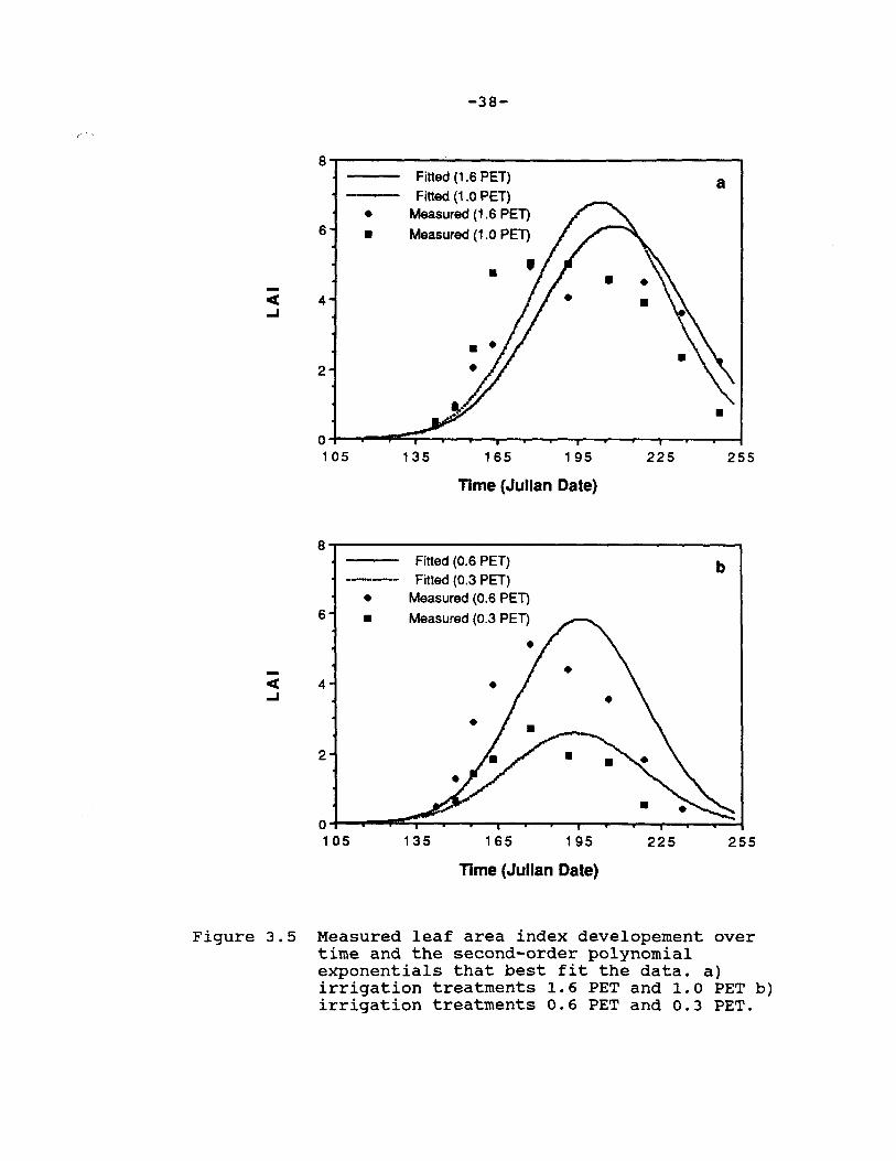
Figure 3.5 Measured leaf area index development over time and the second-order polynomial exponentials that best fit the data. a) irrigation treatments 1.6 PET and 1.0 PET b) irrigation treatments 0.6 PET and 0.3 PET. • . . 38

Figure 3.6 Measured soil water contents in fallow plots under four irrigation treatments on days a) 141 b) 169 c) 197 and d) 225 . . . • . • 44

Figure 3.7 Measured soil water content distributions in plots planted to corn under four irrigation treatments on days a) 141 b) 169 c) 197 and d) 225 .................. 46

Figure 3.8 Comparison of measured soil water contents in the fallow plots with predictions by the Richards equation (R) and the Tipping Bucket routine (T) for Day 141 under four irrigation treatments corresponding to a) 1.6 b) 1.0 c) 0.6 and d) 0.3 potential evapotranspiration (PET) . . . • . . . . • . . . . • . . . 51

xi

Figure 3.9 Comparison of measured soil water contents in the fallow plots with predictions by the Richards equation (R) and the Tipping Bucket (T) routine for Day 182 under four irrigation treatments corresponding to a) 1.6 b) 1.0 c) 0.6 and d) 0.3 potential evapotranspiration (PET) • • • • • • • • • • • • • • • • • • • 5 3

Figure 3.10 Soil water potentials in the fallow plot under irrigation treatment S-03. Comparison of predictions by the Richards equation and measurements by duplicate tensiometers at a) 0.30 m b) 0.45 m c) 0.75 m d) 1.05 m depth ...••.••. 57

Figure 3.11 Comparison of measured soil water contents in the plots planted to corn with predictions by the Richards equation (R) and the Tipping Bucket routine (T) for Day 182 under four irrigation treatments corresponding to a) 1.6 b) 1.0 c) 0.6 and d) 0.3 potential evapotranspiration (PET) .••.•••.. 59

Figure 3.12 Comparison of measured soil water contents in the plots planted to corn with predictions by the Richards equation and the Tipping Bucket routine for Day 225 under four irrigation treatments corresponding to a) 1.6 b) 1.0 c) 0.6 and d) 0.3 potential evapotranspiration (PET) . . . • . . . . . • • • • • 61

Figure 3.13 Effect of moisture release curve parameters on water content predictions fit to whole water potential range (b=l0.1) and fit to wet range only (b=7.8) a) for irrigation treatment 0.3 PET b) 1 . 6 PET • . . . • • . . . . • . . . 6 3

Figure 3.14 Soil water potentials in the cropped plot under irrigation treatment N-03. Comparison of predictions by the Richards equation and measurements by duplicate tensiometers at a) 0.30 m b) 0.45 m c) 0.75 m d) 1.05 m depth •.•••••••••.

Figure 3.15 Soil water potentials in the cropped plot under irrigation treatment N-08. Comparison of predictions by the Richards equation and measurements by duplicate tensiometers at a) 0.30 m b) 0.45 m c) 0.75 m d) 1.05 m

65

depth. . . . . . . . . . . . . . . . . . . 67

xii

Figure 3.16 Soil water potentials in the cropped plot under irrigation treatment N-13. Comparison of predictions by the Richards equation and measurements by duplicate tensiometers at a) 0.30 m b) 0.45 m c) 0.75 m d) 1.05 m depth. . . . . . . . . . . . . . . . . . . 69

Figure 3.17 Predicted total amounts of drainage below 1.20 m and predicted soil evaporation for fallow soil conditions over a range of irrigation water applications. a) predicted by the Richards equation (R) b) predicted by the Tipping Bucket routine (T) •.••.•.. 72

Figure 3.18 Water fluxes below 1.20 m for fallow soil conditions predicted by the Richards equation (R) and the Tipping Bucket routine (T). a) irrigation treatment 1.6 PET b) irrigation treatment 1.0 PET ...••.••..•.. 74

Figure 3.19 Soil evaporation predicted by the Richards equation (R) and the Tipping Bucket routine (T) for fallow soil conditions. a) for irrigation treatments 1.0 PET b) 0.3 PET. 75

Figure 3.20 Total amounts of water contained in the 1.80 m fallow soil profile as measured and as predicted by the Richards equation and the Tipping Bucket procedure. For irrigation treatments a) 1.6 PET b) 1.0 PET c) 0.6 PET and d) 0 . 3 PET . . . . . . • . . • • . . . 7 7

Figure 3.21 Predicted total amounts of drainage below 1.20 m (DR), predicted actual transpiration (TR) and predicted soil evaporation (EV) for cropped soil conditions over a range of irrigation water applications. a) predicted by the Richards equation (R) b) predicted by the Tipping Bucket routine (T) ...•.... 80

Figure 3.22 Partitioning of potential evapotranspiration as predicted by the Richards equation. a) under irrigation treatment 1.0 PET b) under irrigation treatment 0.3 PET ••••••• 81

Figure 3.23 Total amounts of water contained in the 1.80 m soil profile planted to corn as measured and as predicted by the Richards equation and the Tipping Bucket procedure. For irrigation treatments a) 1.6 PET b) 1.0 PET c) 0.6 PET and d) 0.3 PET .......•..•. 83

xiii

Figure 4.1 Crop growth under different irrigation treatments: N-01 (1.6 PET), N-11 (1.0 PET), N-16 (0.6 PET) and S-16 (0.3 PET). a) Leaf area index b) total above-ground dry matter. Error bars represent +1 u ............ 100

Figure 4.2 Leaf area ratios (leaf area/total above-ground dry weight) for different irrigation treatments: A4 (N-01, N-06, S-01), A3 (N-11, S-06), A2 (N-16, S-11), and Al (S-16) ... 102

Figure 4.3 Yield as a function of applied water (PET= 641 mm): a) final dry matter, b) grain yield and index ...•...••

irrigation above-ground c) harvest

103

Figure 4.4 Comparison of measured and predicted crop growth for irrigation treatment N-11 (1.0 PET): a) leaf area and b) accumulated dry matter. Means of leaf area for plants in group A3 (N-11, S-06) +1 u. Also, the measured value for N-11 is included •....... 106

Figure 4.5 Comparison of measured and predicted crop growth for irrigation treatment N-01 (1.6 PET): a) leaf area and b) accumulated dry matter. Means of leaf area for plants in group A4 (N-01, N-06, S-06) +1 u. Also, the measured value for N-01 is included. • 107

Figure 4.6 Comparison of measured and predicted crop growth for irrigation treatment N-16 (0.6 PET): a) leaf area and b) accumulated dry matter. . . . . . . . . . . . . . . . . . 109

Figure 4.7 Comparison of measured and predicted crop growth for irrigation treatment S-16 (0.3 PET): a) leaf area and b) accumulated dry matter . . . . . . . . . . . . . . . . 110

Figure 4.8 Comparison of measured and predicted final top dry matter for irrigation treatments less than PET. . . . . . . . . . . . . . . . . . . . 113

Figure 4.9 Final top dry matter as a function of the amount of irrigation water received. a) simulated and b) measured ••••..••. 114

Figure 4.10 Simulated plant water potential at 14:00 hrs. a) root and b) leaf ..•..•...... 115

xiv

Figure 4.11 Simulated water stress on a daily basis over the growing season for three irrigation treatments N-11 (1.0 PET), N-16 (0.6 PET) and S-16 (0.3 PET). a) ratio of actual to potential transpiration and b) photosynthesis. . • • . • • . • 117

Figure 4.12 Simulated water stress on an hourly basis between irrigation events for treatment N-11 (1.0 PET): a) plant water potential, b) actual and potential transpiration, and c) nonwaterstressed and stressed photosynthesis. 119

Figure 4.13 Simulated water stress on an hourly basis between irrigation events for treatment N-16 (0.6 PET): a) plant water potential, b) actual and potential transpiration, and c) nonwaterstressed and stressed photosynthesis. 122

Figure 4.14 Measured harvest index as a function of accumulated water stress during a) pollination and b) the whole growing season .•.... 124

xv

Chapter I

INTRODUCTION

The Cerrado (Savanna) region of Brazil is an area of

considerable agricultural potential (Abelson and Rowe,

1987; Goedert, 1983). The climate is tropical continental

with rainy summers and dry winters. Annual precipitation

varies with geographical location from 1300 to 1800 mm, of

which 95 % is concentrated in the wet season (September to

April). Climatic conditions are very conducive to the

production of almost any crop. Worldwide, savanna regions

occupy more than twice the surface area as the humid

tropics, and thus represent an enormous resource for

increasing agricultural production.

Initial limitations for agricultural development in

the Cerrado were due to the inherent low fertility and

acidity of the Oxisols and Ultisols, which together

constitute more than 70 percent of the 140 million ha

region. Soil research conducted primarily during the last

20 years has improved understanding of the chemistry and

fertility of these soils and resulted in the establishment

of recommended management practices to alleviate their

inherent soil fertility restrictions (Goedert, 1985).

According to recent estimates, only about five to ten

percent of the estimated 50 million ha of potentially

arable land in the Cerrado is under cultivation (Goedert,

1983) and further development of the region is one of the

-1-

-2-

highest national priorities of the Brazilian government.

With the major soil fertility limitations successfully

identified and correctable by soil amendments, increased

attention is being focussed on the management of other

limiting factors to agricultural production on these

soils, including water and nitrogen.

The foundation for sound management of soils and

development of successful agronomic systems is a thorough

understanding of the physical, chemical and biological

processes that occur in them. While the processes

themselves are not principally different from the

processes studied longer and more intensively in temperate

agriculture, environmental conditions, crops and specific

soil characteristics can differ. Thus empirical knowledge

gained from agricultural research in the temperate regions

can not always be successfully transferred to the

conditions of the Cerrado. However, knowledge of these

processes should, in theory, be applicable to and lead to

further understanding of agriculture in the Cerrado.

Mechanistic simulation models representing and

integrating knowledge about soil-plant-atmosphere

processes are a valuable tool for the transfer of this

knowledge. They can provide a rational framework in which

to design, analyze and evaluate field experiments and

increase our insight into system dynamics. Application of

these models, that have been developed primarily in the

temperate regions, provides the opportunity to discover if

-3-

there are inherent assumptions that do not fit tropical

conditions and thus limit their general applicability.

Such application could lead to improvement in the model

and to a more comprehensive understanding of the important

differences in the properties and dynamics of temperate

and tropical plant-environmental systems.

The specific objective of this research was the

quantitative description of water fluxes in Cerrado soils

in simulation model form. The model was applied to

Cerrado conditions in order to attempt identify the most

important factors determining water fluxes in acid savanna

soils. Furthermore, effects of water stress or surplus

on corn growth and yield were evaluated with the

simulation model. Chapter II describes the software

program GAPS that was developed during the course of this

research and that served to implement the simulation

models used in this work. GAPS was developed with

particular emphasis on flexibility, transparency and user

friendliness. It is intended to be usable for a variety

of purposes ranging from research applications to use in

supporting conceptually oriented teaching. The simulation

model components contained in GAPS are fully documented in

the GAPS User's Manual, version 1.1 of which is contained

in Appendix A.

In chapter III water fluxes in cropped and fallow

soils of the Cerrado are predicted. Two main

representations of soil water flow are compared. They are

-4-

tested against measured data of soil water status obtained

from a line-source sprinkler experiment. The sensitivity

of the model predictions to various important input

parameters is discussed, as well as the implications of

specific soil physical properties of tropical soils with

respect to modeling water flow.

Chapter IV deals with the response of corn growth and

yield to water stress. Predictions of dry matter

accumulation and leaf area development over a wide range

of irrigation water input are compared to data obtained

from a field experiment.

REFERENCES

Abelson, P.H., and J. w. Rowe. 1987. A new agricultural frontier. Science 235:1450-1451.

Goedert, W. J. 1983. Management of the Cerrado soils of Brazil: a review. Journal of Soil Sci. 34:405-428.

Goedert, W. J. 1985. (in portuguese) Solos dos Cerrados. Ministerio da Agricultura / EMBRAPA.

Chapter II

GENERAL PURPOSE SIMULATION MODEL OF WATER FLOW

IN THE SOIL-PLANT-ATMOSPHERE SYSTEM

2.1 INTRODUCTION

Understanding of water movement in the soil-plant

atmosphere continuum (SPAC) has been greatly advanced by

the ability to develop dynamic simulation models that use

numerical techniques to solve equations, based on a

mechanistic view of the system. Such models are essential

to reasonably evaluate how changes in any one component of

the system, such as root depth and density, soil hydraulic

properties, leaf area index, or frequency of rainfall or

irrigation, will affect the water budget of the soil-plant

system. Over the past 15 years many simulation models of

water movement in the soil-plant-atmosphere system have

been developed, as either independent models (Federer,

1978; Goldstein, et al., 1974; Nimah and Hanks, 1973;

Norman and Campbell, 1983). or sub components of larger

models (Davidson et al., 1978; Tillotson et al., 1980).

These models have most often been developed for fairly

specific purposes, such as predicting evapotranspiration

for a particular crop (Campbell et al., 1976; Childs et

al., 1977; Denmead et al., 1976; Running et al., 1975) or

for predicting leaching of solutes in a particular system

(Iskandar and Selim, 1981; Robbins et al., 1980; Wagenet

and Hutson, 1986).

-5-

-6-

Although a particular modeling effort should have a

well-defined purpose, the computer program supporting this

modeling effort need not be written explicitly for this

purpose. The high degree of specificity incorporated into

the code of simulation models is one major reason use of

simulation models by individuals other than those that

developed the model has been extremely limited (Addiscott

and Wagenet, 1985). It might be argued that simulation

models being developed are conceptually very different

from one another and the diversity of models represents

significant differences in the manner in which different

researchers conceive of water movement in SPAC. However,

we would suggest that important conceptual differences in

deterministic models of water movement in SPAC are

relatively few. We believe that development of more

general, flexible simulation models of SPAC will lead to

increased use of these models by those who are not

currently involved in developing them. This, in turn,

will increase the rate of progress in our understanding of

water movement in the soil-plant-atmosphere system.

2.2 APPROACH

The approach we used was to first consider major

reasons that simulation models are not more widely used.

Three reasons appeared most important: 1. most programs

are not flexible enough to accommodate relatively easily a

variety of objectives, 2. most programs are not well

-7-

documented, 3. most programs contain little, if any,

"user-friendly" interfacing. our objective, therefore,

was to develop a software package for simulating water

movement in SPAC that addresses these problems.

There are several aspects of existing simulation

models that make them inflexible. Some require a rigid

set of input data to run; these inputs may not be

available to the user. This, in turn, is due to a lack of

alternative representations of various components of the

model. For example, some SPAC simulation models require

pan evaporation rates as input for calculating

evapotranspiration. The user may not have these data, but

may have other data that could be used for predicting

evapotranspiration. In addition, most SPAC simulation

models do not give the user the option to simulate easily

only parts of the system, such as evapotranspiration or

water flow without evapotranspiration. Our approach was

to create a program that would supply the user with more

than one option to simulate a particular process, the

choice being dependent on available input data, desired

level of complexity, and objectives. GAPS (~enerbl

£urpose ~imulation Model of the Soil-Plant-Atmosphere

system) allows the user to construct a situation-specific

simulation model from existing components. Furthermore,

the program allows users with some programming experience

to add their own components, either to substitute for

existing components or in addition to them, and to link

-8-

them to the existing routines relatively easily.

Clear programming and documentation also support

flexibility and encourage use in several ways. These

features of GAPS allow users with some programming

experience to make changes and add procedures easily.

Good documentation helps the user make educated choices

regarding the selection of model components.

Additionally, such documentation is useful in quickly and

easily determining precisely how the model simulates

various components.

Providing a user-friendly interface between the

simulation model and the user is perhaps scientifically

the least necessary component of GAPS. User-friendly

interfaces can require large amounts of programming in

comparison to the simulation program itself. However,

lack of such an interface could be a major deterrent in

the use of simulation models by a wider group of people.

Our general purpose simulation model is interfaced with

user-friendly menus.

2.3 PROGRAM STRUCTURE

GAPS is divided into three major components: the

editor, simulator, and plotter (Fig. 2.1). The editor

allows the user to create or edit all files that are

necessary input to the simulator. The plotter can be used

to graph or print selected variables from output files

after completion of a simulation run, as well as to print

-9-

(_GA-PS J

START

QUIT MAIN MENU

EDIT SIMULATE PLOT

EDITOR SIMULATOR PLOTIER

QUIT (EXIT TO IBM SYSTEM LEVEL)

Fig. 2.1 GAPS Structure

input data files. Variables printed can be selected by

the user. The simulator contains the library of

procedures from which users can select and design their

own systems (Fig. 2.2).

The GAPS documentation is organized so that every

subroutine/procedure is documented in detail in a separate

chapter. Each chapter includes presentation and

explanation of all equations, using the same symbols as

Air Temperature Solar Angles Atmos Trans

PET Priestly Taylor

Penman Monteith Linacre

Pan

GAPS SIMULATOR LIBRARY

WATER FLOW Richards Eq

Tipping Bucket

WATER UPTAKE Potential Driven PAW Adsorption

PLANT GROWTH Max Photosynthesis

Critical LWP Dry Matter Ace Growth f(time) Growth Stages

f Soil Temperature

Fig. 2.2 currently included simulator modules

I ..... 0 I

-11-

those used in the code, definition of all symbols as they

are presented, explanation of numerical techniques used

where necessary, references to relevant publications, the

procedural code, a dependency diagram where necessary to

illustrate how the procedure is linked to other procedures

and internal flow (Fig. 2.3), and a summary list of all

symbols used in the procedure along with their definition.

In addition to documentation of the procedures currently

contained in the simulator, the GAPS User's Manual

includes instructions on how to change existing procedures

and how to add procedures to the simulator library.

GAPS contains several user-friendly features. First,

the simulator routines in GAPS (the simulator) are linked

to input (the editor) and output (the plotter) routines.

The editor, simulator, and plotter all interface with the

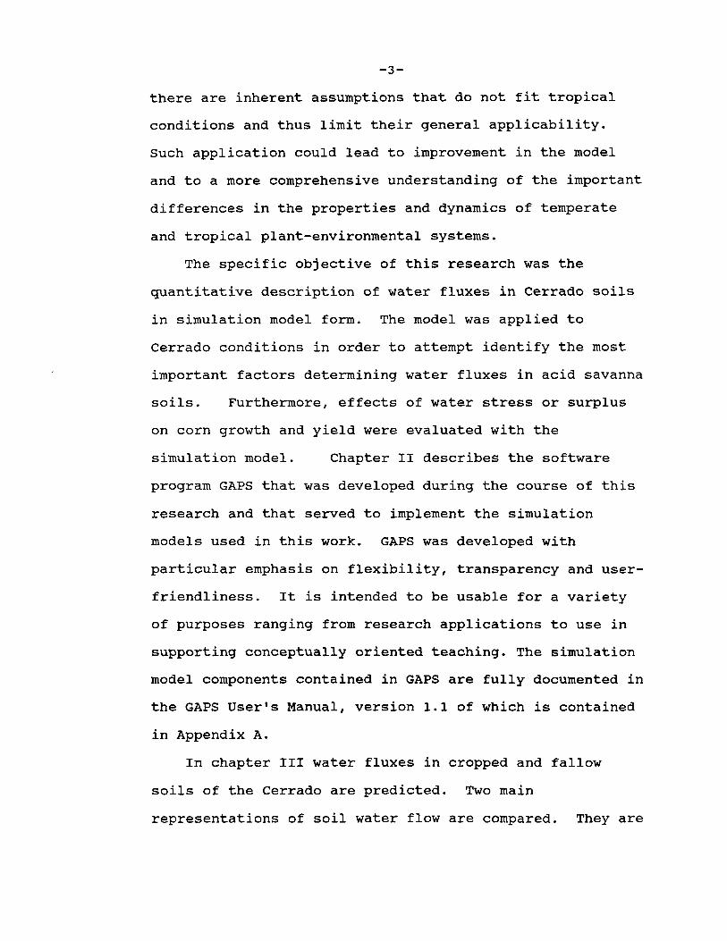
user through a series of menus. The menus have a similar

design (Fig. 2.4) which facilitates a clear presentation

of the options available to the user at any point within

the program. A title section in the upper left-hand

corner of the screen informs the user of the current

location in the program. A menu in the center displays

the options available to the user, for example, to load,

save, edit, or delete a data file while in the editor.

Function keys are utilized for user input. Abbreviated

versions of the options are repeated in the function keys

window. The user has the option to respond by hitting

either the appropriate function key or the first

-12-

Solarflngles

HOUR

24

~SP

HOUR=I

SPRCESUM

Fig. 2.3 Example of Dependency Diagram (Solar_Angles)

-13-

Fig. 2.4 GAPS Screen Menu Format

(highlighted) letter of the respective choice. If there

is user input of text or numbers, the user can enter those

into the user input window. Names of date files that are

currently in memory are displayed in the small window in

the lower right-hand corner of the screen. In addition,

strings used in the GAPS menus were defined in a manner

that involves only minor editing to change them from

English to another language or to change statements in the

menus.

The editor is structured to allow users to create and

edit quickly input files necessary to run the various

-14-

procedures in the GAPS simulator. There is a run-time

plotter associated with the simulator that the user can

use to view simulator results instantly. The user can

choose to view up to four graphs simultaneously.

The user can choose to save simulated output to a file

before running a simulation. The plotter can then be used

after the simulation to plot selected variables from

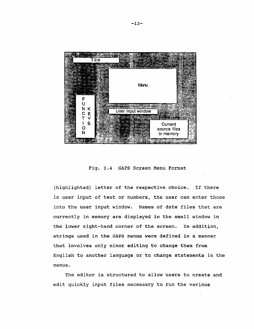
specified output or input files. If desired, GAPS

produces a summary output table containing the names of

input data files, simulation procedures used in the

particular simulation run, and summary water budget

information (Table 2.1). For examples of input data

files, please refer to the GAPS User's Manual (Appendix

A).

2.4 APPLICATIONS

GAPS can be used for a number of different purposes.

As a research tool, GAPS can be used most easily to build

a simulation model for interpreting and analyzing field

experiments. In addition, users can use GAPS as a water

flow shell to which they can add components, such as root

growth models or solute flow models, of major interest to

them. They can also compare different mathematical

representation of the same processes, such as ETP or water

flow, under a particular set of conditions. This can

produce insight into when it is or is not appropriate to

-15-

TABLE 2.1

Example of GAPS summary information table

Simulation started on

Site File Name Soil File Name Climate File Name Plant File Name

Output File Name

8/6/1988 at 11:41

CPAC Oxisol Brasilia 1987 Corn

Testrun

*** Procedures used in simulation ***

Soil Temperature Priestley Taylor ETP Max Photosynthesis Critical Leaf Water Potential Dry Matter Accumulation Growth Stages Water Uptake Richards_Equation

*** Summary data for simulation run ***

Starting day Last day

Total water input (mm) Total potential ET (mm) Total potential transpiration (mm) Total actual transpiration (mm) Total potential soil evaporation (mm) Total actual soil evaporation (mm) Total deep drainage (mm)

Initially in profile (mm) Finally in profile (mm) Change in Storage (mm)

Simulation stopped on 8/6/1988 at 12:52

96 252

327 641 353 250 288 171

4

492 394 -98

-16-

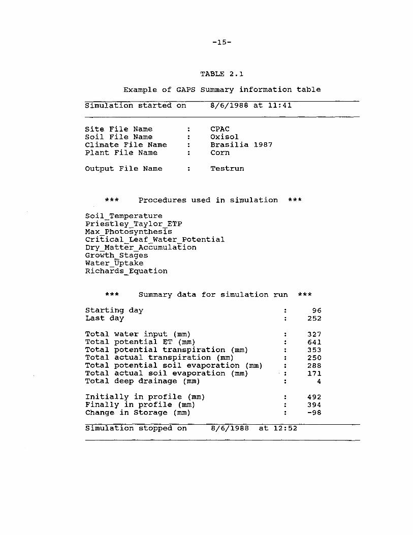
use certain representations of a process.

GAPS can be used as a teaching tool to introduce

students to simulation modeling. Students have the

opportunity to work with individual components of the

system as well as linking components together. They can

explore the effect of changing specific parameter values,

such as saturated hydraulic conductivity, or changing

input data, such as climate files, to see how various

aspects of the water budget, such as evaporation from the

soil surface and movement of water below the root zone,

are changed.

2.5 FUTURE DEVELOPMENT

The core of GAPS is the simulator, which contains the

library of procedures available to construct simulation

models. In this version only procedures relating to water

flow in the SPAC and crop growth procedures have been

included. Work is currently being conducted on simulation

models of nitrogen transformation and transport and

reaction routines that will be incorporated into GAPS. We

envision that those who use GAPS will add or modify

procedures and make these available to other GAPS users.

Some aspects of the current version have been

identified as needing improvement in the future. For

example, using a spreadsheet format in the editor that

will not scroll horizontally limits the number of

variables that can be included in one input data file.

-17-

The plotter is still in the early stage of development.

currently, the editor and plotter, and the global routines

they access, represent the bulk of the GAPS program. In

the future we may consider interfacing the simulator of

GAPS with commonly available database management software

and graphics software.

There appears to be an increasing demand for

simulation modeling of soil-plant-atmosphere systems.

Additionally, development of these models will become

increasingly a multi-disciplinary effort. Such effort

requires clear, fully documented programming and a

programming style as independent as possible to the

author's disciplinary affiliation. A modular structure to

simulation models, such as that represented by GAPS, will

also facilitate multi-disciplinary development and use.

2.6 SOFTWARE AND HARDWARE REQUIREMENTS

GAPS is entirely written in TURBO PASCAL 4.0 and can

be implemented on an IBM PC or PC compatible system with a

graphics adapter, DOS 3.0 or higher and 256K of memory.

REFERENCES

Addiscott, T.M. and R.J. Wagenet. 1985. Concepts of solute leaching in soils: A review of modeling approaches. J. Soil Sci. 36:411-424.

Campbell, M.D., Campbell, G.S., Kunkel, R., and R.I. Papendick. 1976. A model describing soil-plant-water relations for potatoes. Aro. Potato J. 53:431-441.

-18-

Childs, S.W., Gilley, F.R., and W.E. Splinter. 1977. A simplified model for corn growth under moisture stress. Trans. ASAE 20:858-865.

Davidson, J.M., Graetz, D.A., Rao, S.P.C., and H.M. Selim. 1978. Simulations of nitrogen movement, transformation, and uptake in plant root zone. EPA 600/3-78-029.

Denmead, O.T., and B.D. Miller. wheat plants in the field.

1978. Water transport in Agron. J. 68:297-303.

Federer, C.A. 1978. A soil-plant-atmosphere model for transpiration and availability of soil water. Water Resour. Res. 15:555-562.

Goldstein, R.A., Mankin, J.B., and R.J. Luxmoore. 1974. Documentation of PROSPER. A model of atmosphere-soilplant-water flow. EDFB-IBP-73-9, Oak Ridge National Laboratory, Oak Ridge, TN.

Iskandar, I, and H.M. Selim. 1981. Modeling nitrogen transport and transformation in soils. 1. Theoretical considerations. Soil Sci. 131:233-241.

Nimah, M.N., and R.J. Hanks. 1973. Model for estimating soil water, plant and atmosphere interrelations. Description and sensitivity. Soil Sci Soc. Am. Proc.37:522-527.

Norman, J.N., and G.S. Campbell. 1983. Application of a plant-environmental model to problems in irrigation. Adv. Irrig. 2:155-188.

Robbins, c.w., Wagenet, R.J., and J.J. Jurinak. combined salt transport-chemical equilibrium calcareous and gypsiferous soils. Soil Sci. J. 44:1191-1194.

1980. A model for Soc. Am.

Running, s.w., Waring, R.H., and R.A. Rydell. 1975. Physiological control of water flux in conifers: a computer simulation model. Oecologia 18:1-16.

Tillotson, W.R., Robbins, c.w., and R.J. Hanks. 1980. Soil water, solute, and plant growth simulation. Utah Agricultural Experiment Station Bull. 502.

Wagenet, R.J. and J.L. Hutson. 1986. Predicting the fate of nonvolatile pesticides in the unsaturated zone. J. Environ. Qual. 15:315-322.

Chapter III

WATER FLUXES IN ACID SAVANNA SOILS:

A COMPARISON OF APPROACHES

3.1 INTRODUCTION

The ability to quantitatively describe field soil

water fluxes is an important aspect of a wide range of

agricultural and environmental research. Soil water

simulation models have been used to estimate crop

irrigation water requirements (Norman and Campbell, 1983),

to assess the environmental fate of agricultural chemicals

(Wagenet and Hutson, 1986}, and for soil classification

(Van Wambeke, 1985), amongst other purposes. The extent

that simulation models correctly represent the most

important processes and interactions effecting soil water

fluxes in the soil-plant-atmosphere system will determine

their ability to be extrapolated to previously unstudied

locations and conditions.

The ability to extrapolate knowledge across a range of

environmental conditions is particularly important in the

transfer of agricultural technology. While empirical

knowledge is essential in that it provides a valuable body

of information, empirical relationships derived from it

are often site-specific and frequently do not apply across

a range of soils or climates. Mechanistic simulation

models such as the plant-environmental models used in this

research can fill an important role in providing the

-19-

-20-

conceptual framework in which to extrapolate research

results to broad regions as well as aide in the design and

interpretation of agronomic experiments.

The Cerrado region in Brazil is a good example of the

great need to extrapolate agricultural knowledge acquired

in a short time to a large region, in which climatic

conditions and soil properties vary considerably. Most of

the existing understanding of soil and crop management

under Cerrado conditions has been acquired within the last

15 years, when the large-scale agricultural development of

this region was first conceived. Only a few experimental

research sites exist in an area larger than the corn and

wheat belt of the United States.

Furthermore, there are several features of acid

savanna systems that make proper evaluation of water

fluxes critical to sound management. The most unusual

features of highly weathered acid savanna soils in terms

of water movement are their moisture release

characteristics. Although they often exhibit high clay

contents in the order of 50 to 70 % and even higher

(EMBRAPA, 1981) their high degree of aggregation due to

iron and aluminum oxides gives them the drainage

characteristics of sands in the wet range. They are often

referred to as 'pseudo-sands'. At 'permanent wilting

point' (-1500 J kg· 1 ), these soils typically hold between

18 and 22 vol% of water due to their high clay content.

Rapid initial drainage possibly via macropores resulting

-21-

in low water contents at field capacity and high water

contents at 'permanent wilting point' result in very low

amounts of plant available water stored in the soil

profile (Goedert, 1983; Wolf, 1975). Under these

conditions crop rooting depths determine the likelihood of

crop survival during the frequently occurring •veranicos'

or drought periods that occur in the wet season. When

crop rooting depths are restricted by 'chemical

boundaries' such as Al-toxicity or severe Ca deficiency

(Richtey, 1982), not only are the plants more likely to be

subjected to water stress in case of a drought, but

nutrients stored at greater depth are unavailable to the

crop. Yields of corn were shown to be positively related

to the depth of lime incorporation into the soil

(Gonzales-Erica, et al., 1979; Lobato and Ritchey, 1979).

Dry season survival of different legumes species that

might serve to protect the otherwise unused soil surface

against erosion and contribute symbiotically fixed

nitrogen to a succeeding crop appears to be related to

their rooting depths (Bowen, personal communication). If

the roots of acid-tolerant legume species could explore a

deep enough soil profile, chances for surviving the dry

season and resuming growth at the onset of the first rains

would be greatly increased.

Due to the high amounts of rainfall, low cation

exchange capacities and rapid drainage of these soils,

downward movement of Ca within a relatively short period

-22-

of time (several years) has been observed (EMBRAPA, 1978).

The application of gypsum is currently the recommended

method to amend the acid subsoils of the Cerrado. While

the leaching of Ca into the subsoil might well be a

desirable effect, leaching losses of nitrate, potassium

and other cations can be substantial under Cerrado

conditions (Grove, 1979; Richtey, 1979). A better

understanding of the water movement and the leaching

process in these soils is needed (Goedert, 1983) and a

resulting ability to better manage water fluxes will

provide the basis for improved management of soil

amendments and plant nutrients.

Estimates made for the Federal District on the basis

of available water resources predict a potential for

irrigation of five to ten percent of the total land area

(Pruntel, 1975). Quantification of water fluxes in

Cerrado soils is an essential prerequisite for irrigation

project planning and management. studies have been

conducted to quantify irrigation water requirements of

Cerrado crops (Luchiari, 1988). This information should

be in a form that can be extrapolated from research

station experiments to other acid savanna soils and

climatic conditions within the Cerrado or elsewhere

(Goedert, 1983). Simulation models will provide a valuable

tool to increase understanding of the interactions between

soil physical properties, water dynamics and crop growth

under Cerrado conditions.

-23-

This research had as it's major objective the

quantitative description of water fluxes in Cerrado soils

under cropped and fallow conditions. A field experiment

was conducted at the Centro de Pesquisa Agropecuaria dos

Cerrados (CPAC) near Planaltina, Brazil from April to

September 1987 to collect data on the water budget of acid

savanna soils under a wide range of irrigation water

inputs. Data obtained from this field experiment was

compared to simulated data using two soil water simulation

models. The General Purpose Simulation Model GAPS

(Buttler and Riha, 1987, 1988) was used to implement

alternative simulation model representations and to

compare the effect of their respective assumptions and

limitations on model performance. Two major alternative

approaches to model soil water flow, the Richards equation

(Campbell, 1985) and the Tipping Bucket method (Jones and

Kiniry, 1986; Ritchie et al., 1986}, were compared in

their ability to predict measured soil water contents and

soil water potentials (for Richards equation only).

Specific objectives were to test the hypotheses and

assumptions contained in two alternative representations

of water flow in the soil and their resulting ability to

predict within reasonable range of error soil water

contents in cropped and fallow soils subjected to a wide

range of water inputs.

-24-

3.2 MATERIALS AND METHODS

3.2.1 Line Source Irrigation Experiment

The experimental site was located on the EMBRAPA-CPAC

(Cerrado Agricultural Research Center) research station in

the Federal District of Brazil, latitude of 15.5 degrees

south and longitude of 27.5 degrees west, at an altitude

of 1000 m. The soil is classified as an Oxisol (Typic

Haplustox, isohyperthermic, fine, kaolinitic) or a Dark

red Latosol in the Brazilian classification system (Macedo

and Bryant, 1987). Corn (Zea mays L., 'Cargill 111 S')

was planted on 21 April 87 in 80 cm wide rows at a final

population density of 62,500 plants/ha. The crop was

grown during the dry season in order to have optimal

control of irrigation water treatments.

A line-source sprinkler irrigation system (Hanks et

al., 1976) was used to establish a gradient of irrigation

water application across a plot perpendicular to the

irrigation line. Irrigation water was applied at the same

frequency to all plots, but at rates ranging from

approximately 3 to 25 mm hour· 1 • Quantities of applied

water were measured after each irrigation event with catch

cans located between the corn rows just above the crop

canopy. Three rows of 40 catch cans each spaced

approximately 15 meters apart were used to collect the

irrigation water. Uniformity along the irrigation line

was relatively good, with coefficients of variation

generally around five percent. This allowed the mean of

-25-

the three sampling locations to be used to represent

amounts of irrigation water applied as a function of

distance from the line source. Wind conditions led to a

consistently different distribution of water between the

two halves of the experimental field, prohibiting treating

plots on opposite sides of the irrigation line as

replicates.

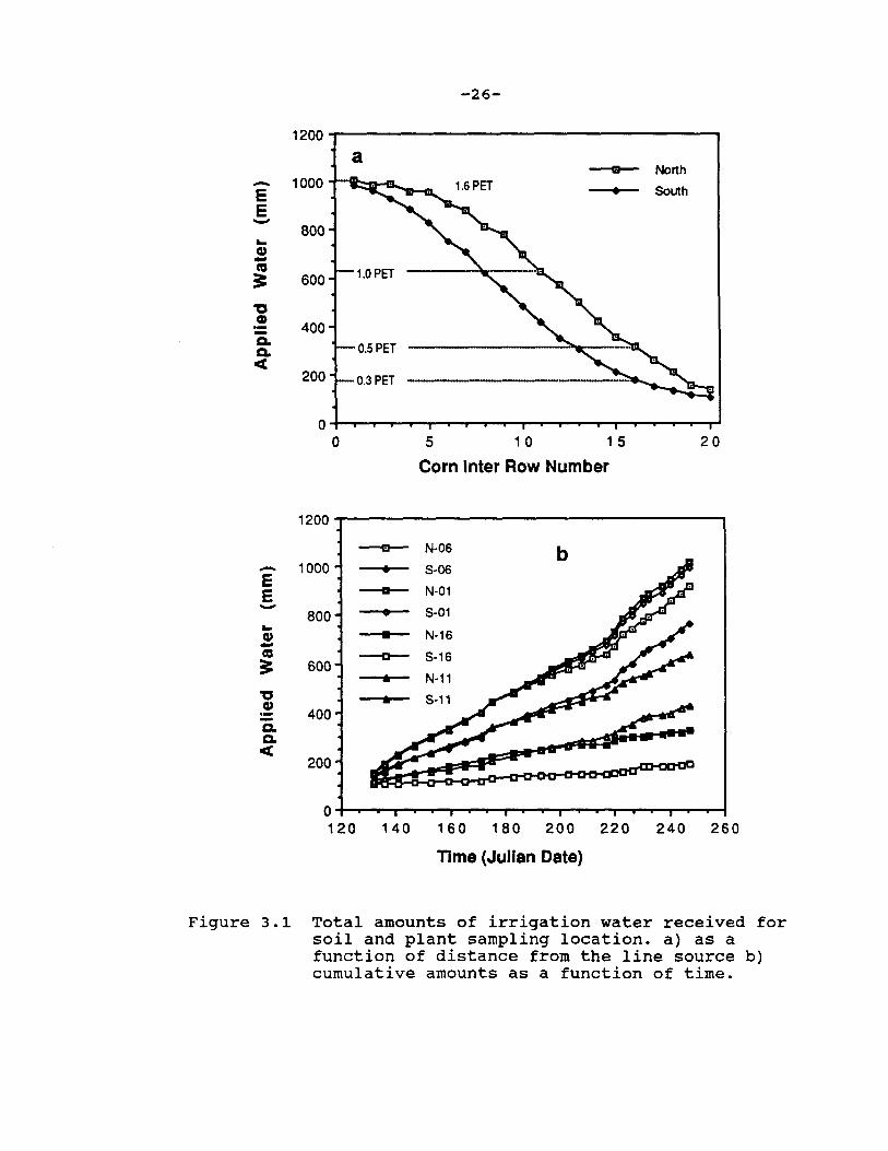
Irrigation water was applied every three to five days

for two to three hours after dusk, when wind speed was

low. Accumulated irrigation water application for all

eight soil sampling locations is presented in Fig. 3.la.

The total amount of irrigation water received at the two

extreme sampling locations during the experimental period

(including 104 mm natural precipitation) was 105 mm (S-16)

and 1020 mm (N-01) (Fig. 3.lb). Comparisons between

measured and predicted data will be discussed for four

irrigation treatments (N-01, N-11, N-16, and S-16),

representing approximately 1.6, 1.0, 0.6, and 0.3 of

potential evapotranspiration (PET), respectively, when

averaged over the whole growing season.

Treatments perpendicular to the irrigation line

consisted of three different nitrogen (N) fertilizer

application rates (O, 100, and 200 kg N/ha) planted to

corn and replicated twice on each side of the sprinkler

line and two non-replicated fallow plots. Only the

results from the cropped treatment receiving 200 kg N/ha

nitrogen fertilizer and the fallow treatments are reported

-26-

1200

a - North - 1000 1.6 PET E South

E - 800 ... Cl) -ta 1.0 PET 3: 600

,:, Cl)

400 a. 0.5 PET a. < 200 0.3 PET - .......... ··-·

0 0 5 1 0 1 5 20

Corn Inter Row Number

1200 - N-06 b - 1000 • S-06 E

N-01 E a - S-01 800 ... N-16 Cl) • -ta D--- S-16

3: 600 • N-11

,:, • S-11 Cl) ·- 400 -a. a. < 200

0 120 140 160 180 200 220 240 260

Time (Julian Date)

Figure 3.1 Total amounts of irrigation water received for soil and plant sampling location. a) as a function of distance from the line source b) cumulative amounts as a function of time.

-27-

in this chapter.

3.2.2 Soil and Plant sampling

Soil samples were collected every two weeks between

specified corn rows. Of the twenty rows of corn on each

side of the sprinkler line (numbered 1 to 20 starting at

the irrigation line) rows 1/2, 6/7, 11/12, and 16/17 were

designated as soil sampling locations to represent

different water regimes along the continuous gradient of

water application across the plot. The sampling locations

will be referred to as N-01, N-06, N-11, and N-16 for the

northern side of the experimental field and as s-01, S-06,

S-11, and S-16 for the southern side. Soils were sampled

a total of nine times during the experimental period and

the water content determined gravimetrically.

Additionally, a neutron probe was used during the later

part of the season to support the gravimetric sampling

scheme. 48 mercury tensiometers were installed in two

blocks (blocks 4 an~ 14) in three maize rows (rows 3, 8,

and 13) at depths of 0.30, 0.45, 0.75, and 1.05 min

replicates of two and were read daily to obtain

measurements of soil water potential.

Sequential harvests of the above-ground part of the

maize plants were made weekly for the first five weeks

starting 30 days after emergence and then biweekly on the

same days as the soil was sampled. Leaf area was measured

using a leaf area meter.

-28-

3.2.3 Simulation Procedures

Two different soil water transport models were used to

simulate soil water content distributions over time and as

a function of depth under the different irrigation

treatments. The ~enerAl ~rpose ~imulation Model (GAPS)

(Buttler and Riha, 1987, 1988) was used to compare two

main approaches to the simulation of soil water movement:

a numerical solution to the Richards equation (Campbell,

1985) and a capacity-type water budgeting routine adapted

from the CERES Maize model water flow routine (Jones and

Kiniry, 1986; Ritchie, et al., 1985) and incorporated into

GAPS as the 'Tipping Bucket' water flow procedure.

Detailed documentation of the two water flow procedures

with explanations of governing equations and their

solutions is contained in the GAPS User's Manual (Buttler

and Riha, 1988, Appendix A).

The Priestley-Taylor equation (alpha= 1.26) was used

to estimate potential evapotranspiration (Priestley and

Taylor, 1972), which was partitioned into potential soil

evaporation and potential transpiration using an equation

presented for corn by Stockle and Campbell (1985). For

simulating plant water uptake, two different water uptake

procedures compatible with the water flow simulation

procedures were used. In the case of the Richards

equation, which predicts hourly changes in soil water

potentials, a potential-driven plant water uptake

procedures was used to estimate root water uptake and

-29-

actual transpiration (Riha and Campbell, 1986). Actual

transpiration is determined by the response of stomatal

resistance to leaf water potential (Fisher et al., 1981),

assuming a critical leaf water potential of -1400 J kg· 1 •

Water flow into roots was assumed to be inversely

dependent on the resistance to water flow in the soil and

in the root (Gardner and Ehlig, 1962). Water flow from

the bulk soil to the root is directly dependent on the

gradient between roots and soil water potentials (Gardner,

1960). The root water potential was not allowed to drop

below -1500 J kg· 1 • Soil evaporation is incorporated into

the Richards equation as proposed by Campbell (1985), with

actual soil evaporation being controlled by the humidity

at the evaporating surface during first stage drying and

by the liquid flux to the evaporating surface during

second- and third-stage drying.

The Tipping Bucket procedure was combined with a plant

water uptake routine based on the concept of plant

available water. Plant water uptake from any layer in the

soil containing roots is allowed to proceed until a lower

limit of plant-extractable water (permanent wilting point)

is reached. The root density distribution in the soil

profile is used to partition the transpirational demand

between soil layers. Demand not met in any one layer is

transferred to other layers as an additional demand. Root

densities thus do not limit root water uptake in this

simple representation, but serve solely to partition

-30-

transpiration in the soil profile. Soil evaporation was

included in the Tipping Bucket water flow procedure as

simple first-stage evaporation, which was allowed to

proceed until the soil water content reached 50 % of its

value at permanent wilting point. Soil evaporation

occurred only from the surface soil node. No upward water

flow was simulated in the Tipping Bucket water flow

routine. An hourly time step was used for both water flow

models. Simulations were conducted from 06 April 87 (Day

96), starting with a measured water content distribution,

to 09 September 87 (Day 252).

3.2.4 Simulation Input Data

3.2.4.1 Climate and Location Data

Daily climatic data for the experimental site was

obtained from CPAC's main meteorological station located

approximately 50 m away from the experimental location.

Climatic data include daily precipitation (mm), Class 'A'

pan evaporation (mm), solar radiation (cal m· 2 day· 1 ),

daily average wind speed (m s· 1 ), maximum and minimum air

temperature (°C), maximum and minimum relative humidity.

The climate file for the experimental period containing

the above variables is included as Appendix B. Daily

minimum and maximum air temperatures and daily total solar

radiation were transformed into hourly values (see GAPS

Manual, Appendix A).

-31-

3.2.4.2 Soil Parameter Estimation

Soil physical properties were characterized to the

extent that they were needed as inputs to the water flow

routines. Soil particle density and texture was

determined on soil samples collected from three randomly

chosen locations in the experimental field in 0.15 m depth

intervals to a depth of 1.80 m (Gee and Bauder, 1985).

Mean soil clay, silt, and sand percentages were 58.7

(1.8), 6.0 (1.1), and 35.3 (1.3) percent, with the numbers

in parenthesis being the standard deviations. The mean

particle density was 2.66 Mg m· 3 (0.02 Mg m·3).

Differences in soil texture and particle density were not

significant between depths.

Dry bulk density and hydraulic parameters were

measured on undisturbed soil cores. A pit (2 m by 1.5 m)

was excavated in the border area of the experimental field

to a depth of 1.85 m. Twelve soil cores per depth (depth

increments corresponding to later soil sampling depths)

were collected along the 2 m face of the pit. A total of

110 core samples was collected. An additional 80 core

samples were collected to a depth of 0.65 mat four other

sites randomly chosen within the experimental field, to

test for within field variability. Bulk densities and

hydraulic conductivities measured on the latter 80 samples

did not differ from the samples collected in the deep pit,

and are not reported.

-32-

Soil saturated hydraulic conductivity was determined

on the cores using the constant head method (Klute and

Dirksen, 1985). The weight of the soil cores was

determined immediately after each conductivity measurement

to obtain an estimate of the relative saturation of the

sample during the determination of saturated hydraulic

conductivity. The degree of saturation during the

determination of saturated hydraulic conductivity on the

50 core samples, for which soil moisture release

parameters were later measured, ranged from 89% to 101% of

calculated total porosity (Table 3.1). Soil bulk

densities showed increased values at the 0.15 to 0.45 m

depths probably due to compaction. The higher soil bulk

densities were highly negatively correlated with measured

saturated conductivities (Fig. 3.2).

Saturated hydraulic conductivities measured in the

laboratory compare well with values reported by others for

the same soil under field conditions (EMBRAPA-CPAC, 1981).

A value of 125 cm day· 1 (0.00148 kg s m·3) was a field

measured value for satiated hydraulic conductivity

reported by Luchiari (1988) and is well in the range of

the conductivity measured in the soil layer with the

highest bulk density (0.0016 kg s m· 3 ). Bouldin (1979)

reported infiltration rates between 17 and 22 cm hour·1

(0.004 and 0.006 kg s m· 3 , respectively), which is also in

agreement with the laboratory measurements.

-33-

TABLE 3.1

Soil physical parameters (mean, standard deviation, maximum and minimum values for 50 soil cores from 9 depths (0.07 - 1.85 m).

Parameter

Bulk density (Mg m· 3 )

Total porosity (m3 m· 3 )

sat. hydr. conductivity

(kg s m· 3 )

Water content (m3 m· 3 )

Degree of saturation

(%)

1. 051

0.605

0.00424

0.567

0.938

u Min Max

0.084 0.932 1.295

0.032 0.513 0.649

0.00178 0.000369 0.00723

0.030 0.485 0.618

0.031 0.891 1. 01

Moisture characteristic curves were determined on 60

of the above 110 core samples using pressure plates

(Klute, 1985 c) (Fig. 3.3). Soil water potentials below

the air entry potential are described as a function of

soil water content using an equation proposed by Campbell

(1974,1985): WP= AE (WC/Ws)·b, where WP is the soil

water potential (J kg· 1 ), WC is the soil water content (m3

m· 3 ), WS is the saturation water content (m3 m· 3 ), AE is

the air entry potential (J kg· 1 ) and bis the soil-B

value. AE and B can be determined from moisture release

data by plotting log(WP) against log(WC/WS) and fitting a

best fit line to the data. One set of soil b-values and

air-entry potentials was calculated using only the

-20

-50 -E ()

-80 -.J:. -a. -110 Cl)

C

-140

-170

-200 0.90

-20

-50 -E () - -80

s:. -2° -110 C

-140

-170

-34-

Bulk Density (Mg/m3)

Iii

a

m

II

m

1---G>---t

1--G--1

m

0.95 1.00 1.05

6 • b

6 •

• arithmetic mean

A geometric mean

1.1 0

6 •

I 0

m

1. 15

Iii

1.20 1.25 1.30

-200 -+--~-~--.---.-------.----...... ---.--.....f 0.002 0.004 0.006 0.008 0.010

KS (kg s m-3)

Figure 3.2 Soil physical properties measured on 110 undisturbed soil cores. a) bulk densities b) laboratory measured saturated hydraulic conductivities.

-C) ~ --.., .....

-C II -0

Q. .. II -Ill

31:

0

-200

-400

-600.

-800

-1000

-1200 ·

-1400

-35-

Water Content (m3/m3)

•

•

1 I I Ii II I •

• •

-1600-+-..--...---,,.....,..-,.-....._. __ ,.._,,_..,_.._. _____ ..........,

0.22 0.27 0.32 0.37

Figure 3.3 Soil moisture release curve. Data points represent means of 60 sample± 1 u taken to a depth of 1. 85 m.

-36-

water content/water potential data for the wet range (-6

to -100 J kg· 1 ) (Fig. 3.4a), and a second set of

parameters was obtained from fitting the equation over the

whole range from -6 to -1500 J kg· 1 (Fig. 3.4b), using

mean water contents and potentials over all depths.

Input data for the Tipping Bucket water flow routine

were calculated from moisture release data. The

volumetric water content at -33 J kg· 1 (0.272 m3 m· 3 ) was

used as the Drained Upper Limit (DUL) or 'field capacity'

and the volumetric water content at -1500 J kg· 1 (0.20 m3

m· 3 ) as the Lower Limit (LL). The Profile Drainage

Constant and other parameters used in the Tipping Bucket

procedure were calculated according to the equations given

by Ritchie et al. (1986). The soil input data file used

for the simulations is presented in Table 3.2.

3.2.4.3 Plant Input Data

For the purpose of the water budget simulations

presented in this chapter, plant growth was treated as an

input to the model rather than being simulated. Second

order polynomial exponentials were fit to the measured

leaf area data obtained from the sequential harvests (Fig.

3.5). For this purpose the eight sampling points (N-01 to

S-16) were grouped into 4 classes according to the amounts

of irrigation water they received. Empirical equations

were then used in the model to estimate leaf area index as

-C) .lll: -.., -'ii ::. C G) -0

CL

... G) -ca 3: C) 0

-C) .lll: -.., --ca ::. C G) -0 CL

... G) -ca 3: C) 0

-37-

Moisture Release Curve 8

li1 a 7 Iii

6

5

li1 4

3 b = 10.31

2 AE = • 0.42 J/kg

-0.6 -0.5 -0.4 -0.3 -0.2

log (WC/WS)

5-,---------------------b

4

3

b = 1.n 2 AE = -0.30 J/kg

1T"---,.--"T"9-~--T"--"""'T'--~-"""'T'----I -0.6 -0.5 -0.4 -0.3 -0.2

log (WC/WS)

Figure 3.4 Soil moisture release parameters for the Campbell equation. Fit to a) the whole range (-6 to -1500 J/kg) of water potentials b) to the wet range only (-6 to -100 J/kg).

-38-

8 Fitted (1.6 PET) a Fitted (1.0 PET)

• Measured (1.6 PEn 6 • Measured (1.0 PEn

• ~ 4 • .J

• 2

0 +---t===:::;:.--T----,,--..,.....--,--,---,---,.-T--_ _, 1 05 135 165 195 225 255

Time (Julian Date)

8 Fitted (0.6 PET) b ---·--- Fitted (0.3 PET)

• Measured (0.6 PEn 6 • Measured (0.3 PEn

~ 4 • .J

• 2

• 0 105 135 165 195 225 255

Time (Julian Date)

Figure 3.5 Measured leaf area index developement over time and the second-order polynomial exponentials that best fit the data. a) irrigation treatments 1.6 PET and 1.0 PET b) irrigation treatments 0.6 PET and 0.3 PET.

-39-

TABLE 3. 2

Soil input data file

Soil File Name Oxisol Soil Name Dark Red Clay 60 % Particle Density 2.66 Mg Soil b-value 10.31 Air Entry Pot. -0.42 J

Drained Upper Limit 0.30 m3 Lower Limit 0.20 m3

Node Depth BD KS (m) (Mg m· 3 ) (kg s m· 3)

1 0.01 1. 07 0.0026 2 0.08 1. 07 0.0026 3 0.23 1. 22 0.0016 4 0.38 1.15 0.0031 5 0.53 1.07 0.0039 6 0.75 1. 00 0.0054 7 1. 05 1.00 0.0061 8 1. 35 1. 00 0.0061 9 1. 65 1. 00 0.0050

10 1.85 1. 00 0.0035

Latosol

m· 3

kg· 1

m· 3 m· 3

Initial WC (m3 m· 3)

0.32 0.32 0.31 0.31 0.28 0.27 0.27 0.27 0.27 0.27

the sample was used to determine relative root density

distributions in the soil profile. The maximum rooting

depth observed in the high water/high nitrogen treatments

was 1.20 m. More than half of the total root weight in

the 90 cm soil profile was concentrated in the uppermost

15 cm. Root densities reported by Gonzales-Erice (1979)

for the same location and corn variety were 4.6 to 5.1 cm

cm3 under limed conditions and consequently, a root length

value of 5.0 cm cm3 was assumed for the Oto 15 cm depth

increment. Root densities were than reduced with depth

using the measured relative root distribution. To

-40-

simulate root growth, the crop growth components included

in GAPS and based on a simulation model developed by

Stockle and Campbell (1985) were used. They are described

in greater detail in chapter IV and fully documented in

the GAPS user's manual (Appendix A). Rooting depth was

simulated on the basis of simulated daily dry matter

partitioned to roots (Foth, 1962). Instead of changing

root densities in each layer over time, a static root

density distribution was used and additional layers were

activated as the season progressed in accordance with the

simulated rooting depth. The plant input data used is

presented in Table 3.3.

3.2.5 Statistical Analysis

Statistical analysis of the experimental data was

performed using the Statistical Analysis System (SAS

User's Guide, 1985). The main objective of the

statistical analysis of the measured water content data

was to obtain a mean and standard deviation of soil water

content as functions of applied irrigation water and as a

function of time and depth. These measurements were than

compared to data obtained from the simulation model.

Multivariate analysis of the soil water content data

was performed using the REPEATED MEASURE OPTION in PROC

ANOVA, treating measurements over depth as repeated

measures and performing the analysis for each sampling

-41-

TABLE 3.3

Plant input data

Plant File Name Plant Name

Emergence date Initial LAI Minimum root water potential Root radius Root resistance Initial canopy height Aerodynamic resistance (RA) Short-wave absorptivity (AS) Critical leaf water potential

Soil profile node

1 2 3 4 5 6 7

. .

: . .

:

Root (m

1. 0 5.0 3.0 1. 0 0.6 0.4 0.2

Corn Cargill 111 s

117 (Julian date) 0.07 -1500 J kg" 1

0.002 m 2.5E+10 kg s m· 4

0.10 m 40.0 s m· 1

0.70 -1400 J kg· 1

Density m· 3)

E+04 E+04 E+04 E+04 E+04 E+04 E+04

date. IRRIGATION was treated as nested within SIDE due to

the differences in irrigation water application rate

between sides. To test for the effect of IRRIGATION

(SIDE), p-values were hand-calculated using the

appropriate mean square error for the overall model.

Expecting the water contents over depths of sampling

to be correlated, Wilk's criterion was used to test for

differences among treatments. The advantage of employing

a multivariate technique is that a statement can be made

about the correlation of a number of variables that are

-42-

studied simultaneously. The 'within subject effects' thus

relate to the changes in water contents with depth. The

'between subjects effects' test the hypothesis that the

between subject factors (e.g. irrigation treatment,

nitrogen treatment) have no effect on the dependent

variables ignoring the within subject effect in the

design. The test sums over the dependent variables, in

this case it sums the water contents over all sampling

depths and tests hypotheses relating to the effect of a

treatment for water content on the average.

3.3 RESULTS AND DISCUSSION

3.3.1 Water Content Distribution in the Soil Profile over

Time under Various Irrigation Treatments

The initial soil sampling on 06 April showed very

little variability in soil water content distribution in

the field with coefficients of variation ranging from one

to two percent. This sampling occurred 20 days after the

grass sod previously covering the experimental area had

been broken and 15 days before planting. By May 07, 16

days after planting, but before the first irrigation water

application, water contents still varied very little.

Rainfall and one uniform application of irrigation water

were sufficient to provide adequate moisture for

germination.

-43-

3.3.1.1 Fallow Treatments

Fig. 3.6 depicts the progression of measured soil

water contents and their profile distribution with time

under the four representative irrigation treatments,

corresponding to approximately 1.6 (N-01), 1.0 (N-11), 0.6

(N-16) and 0.3 (S-16) potential evapotranspiration. The

difference in amounts of irrigation water applied led to a

clear separation of water contents which became more

pronounced with time. Since the fallow plots were not

replicated, no statistics are presented.

3.3.1.2 Cropped Treatments

On Day 141, nine days after the first and four days

after the second irrigation water application, irrigation

water treatment (IRRIG) already showed a significant

effect on water contents in the profile. Throughout the

soil profile to a depth of 1.80 m, IRRIG (SIDE) was

significant at p=0.0001 and remained significant

throughout the soil profile for water contents throughout

the season (Fig. 3.7).

These results show that the experimental design and

data collection scheme was able to provide statistically

significant differences in measured soil water contents

between the sampling locations selected along the

continuous gradient of irrigation water application. This

is an important prerequisite for a meaningful comparison

of these measured data with simulation model output.

-44-

Figure 3.6 Measured soil water contents in fallow plots under four irrigation treatments on days a) 141 b) 169 c) 197 and d) 225.

-0.50

e -= -1.00 Q. • Q

-1.50

Soll Water Content (m3 m-3)

a

----- 1.6 PET

-- 1.0PET

-- 0.6PET

--- 0.3PET

DAY 141 21 May 87 Fallow

-2.00 +-....-....., ............ __,... ...... _..,....y--.,........,,.....,--.,-.,.._...__..,.......1

0.15 0.20 0.25

-0.50

e ......

= -1.00 Q. • Q

-1.50


C

-- 1.6PET

- 1.0PET

-- 0.6PET

--- 0.3PET

0.30

DAY 197 16 July 87 Fallow

0.35

-2.00 -t-...-..--...... --,.--.-............ ..,....T'"""...-,-..,--.-y--,-....--.........1 0.15 0.20 0.25 0.30 0.35

-0.50

...... E -= -1.00 Q. • Q

-1.50


b

-- 1.6PET

-- 1.0PET

-- 0.6PET

-- 0.3PET

DAY 169 18June87 Fallow

-2.00 +-.....-..-..-,,....,--.--.-.---r-...,.......,.... __ ...-..-.,........, ............ -J

0.15

-0.50

e = -1.00 Q. • Q

-1.50

0.20 0.25 0.30


d

DAY 225 13 August 87 Fallow

-- 1.6PET

-- 1.0PET

-- 0.6PET

-- 0.3PET

0.35

-2.00 -+--.-..-_.-.............. --.-.---r--.--.-....... --...------' 0.15 0.20 0.25 0.30 0.35

I

""' 01 I

-46-

Figure 3.7 Measured soil water content distributions in plots planted to corn under four irrigation treatments on days a) 141 b) 169 c) 197 and d) 225.

-0.50

e ......

= -1.00 a. GI C

-1.50


•

-------- 0.3PET DAY141 21 May 87

-2.00 -+-..-....-........................... ---............. -..-..--....... ,......,--f

e ...... :c IQ. w C

0.15 0.20 0.25


-+- 0.3PET

0.30

DAY 197 16July87

0.35

-2.00 +-...-..-....-............. - ............ -------....--....... ....-1 0.15 0.20 0.25 0.30 0.35

-0.50

e ...... = -1.00 a. GI C

-1.50


b

-------DAY 169 18June 87

-2.00-+-....... ..-....-......, .............. ___________ ......J

0.15 0.20 0.25 0.30 0.35


e ...... s:; -a. I)

C

DAY 225 13 August 87

-2.00 +--.--,--,.......,,.....,......,._ ...... _,--...--,.......,,...... ..... _ ...... _._.i

0.15 0.20 0.25 0.30 0.35

I ~ '1 I

-48-

3.2.2 Comparison of Predicted and Measured Soil Water

Contents and Potentials

3.2.2.1 Fallow Treatments

Initial model execution using the Richards equation

indicated that simulated soil water contents were

consistently higher then field-measured values. It was

concluded that the assumption that field saturated water

content is equal to total porosity was not valid for this

soil, which has bulk densities around 1.00 Mg m· 3 and

approximately 15% of total porosity is macroporosity

(Luchiari, 1988). Although saturation percentages of

about 95 % (85-100) were obtained during measurements of

saturated hydraulic conductivity on undisturbed soil cores

in the laboratory (see Table 3.1), the soil does not reach

these high values under field conditions. Luchiari (1988)

reported field saturated or 'satiated' water contents of

about 0.47 m3 m· 3 measured on the same soil in close

proximity to this experiment's location. This would

correspond to a saturation percentage of 75 % of total

porosity at a bulk density of 1.00 Mg m· 3 • The highest

volumetric water contents ever measured in the field

during this experiment were in the range of 0.35 to 0.37

m3 m· 3 •

Using 70 % of total porosity as a saturation water

content yielded satisfactory results for most of the

profile layers, except for those layers that exhibited

increased bulk densities due to compaction. Increasing

-49-

bulk density leads to lower predicted water contents at

the same soil water potential when all other soil

parameters are held constant. This is due to the decrease

in soil pore volume, calculated from measured bulk and

particle densities. In reality, measured soil water

contents at the 15-30 and 30-45 cm depth increments were

consistently higher during the entire season than water

contents below and above these layers (see Fig. 3.7). It

was hypothesized that the process of compaction leads

first to a loss of macroporosity. A loss of 10 to 20

percent of macroporosity might not lead to a proportional

decrease in saturation water content, which is implicit in

using a fraction of total porosity as the field saturation

water content. It was decided to use 70 % of total

porosity (0.43 m3 m· 3 ) throughout the soil profile, except

for the layers exhibiting higher bulk densities, for which

a fraction of total porosity equivalent to a field

saturated water content of 0.43 m3 m· 3 was calculated. It

was assumed that the loss of macroporosity reflected in

increased bulk densities did not result in an equivalent

decrease in field saturated water content. This

adjustment of the field saturation water content was

performed using a subset of the experimental data, namely

the highest irrigation treatment of the fallow plot. The

air entry potential was recalculated assuming the field

saturated water content ws in equation (1). The

relationship of the log of soil water potential to the log

-50-

of soil water contents is not linear over the whole range

of soil water potentials for this particular soil. When

the Campbell equation is fit to the range from -6 to -1500

J kg· 1 , water contents at the wet end of the moisture

release curve will be under predicted, while it provides a

reasonable fit at low water potentials. Soil water

content predictions can be improved in the high water

content range, when using parameters fit to moisture

release data to -100 J kg· 1 , only (see Fig. 3.4). The

choice of the range of water potentials to which to fit

the parameters has a strong effect on their values,

particularly on the value for B (in equation 1).

Results of the comparison between predicted and

observed soil water contents for the fallow plots under

the four irrigation treatments using the moisture release

parameters obtained from fitting equation 1 to the full

range of water potentials are shown in Fig. 3.8 (Day 141)

and Fig. 3.9 (Day 181) for the fallow soil. Comparisons

between the predictions made by the two water flow models

used and the measured data are presented for two sampling

dates. The two sampling dates on day 141 and 182 occurred

5 and 6 days after the last irrigation treatment,

respectively. Agreement between the Richards equation and

measured values is generally good with differences between

measured and predicted soil water contents generally

around 1-3 volume percents for all the sampling dates.

-51-

Figure 3.8 Comparison of measured soil water contents in the fallow plots with predictions by the Richards equation (R) and the Tipping Bucket routine (T) for Day 141 under four irrigation treatments corresponding to a) 1.6 b) 1.0 c) 0.6 and d) 0.3 potential evapotranspiration (PET).

Soll Water Content (m3 m-3) Soll Water Content (m3 m-3)

0.00 0.00

a b

Fa now ( 1.6 PEl) Fallow (1.0 PE1)

-0.50 Day 141 -0.50 Day 141

21 May 87 - 21 May87 - E E --.c -1.00

.c -1.00 -- Q. Q. • • C C

-1.50 - Measured -1.50 - Measured

--0-- Predicted (R) ---o-- Predicted (A) -- Predicted (1) --....-- Predicted (1)

-2.00 -2.00

0.15 0.20 0.25 0.30 0.35 0.40 0.15 0.20 0.25 0.30 0.35 0.40 I

U1 IIJ I

Soll Water Content (m3 m-3) Soll Water Content (m3 m-3) 0.00 0.00

C d

Fallow (0.6 PE1) Fallow (0.3 PE1) -0.50 Day 141 -0.50 Day 141 - 21 May87 - 21 May87

E E - -.c -1.00 .c -1.00 - -Q. Q. ., • C C

-1.50 -- Measured -1.50 -- Measured - Predicted ( R) - Predicted (R) - Predicted (1) -- Predicted (1)

-2.00 -2.00 0.15 0.20 0.25 0.30 0.35 0.40 0.15 0.20 0.25 0.30 0.35 0.40

-53-

Figure 3.9 Comparison of measured soil water contents in the fallow plots with predictions by the Richards equation (R) and the Tipping Bucket (T} routine for Day 182 under four irrigation treatments corresponding to a) 1.6 b) 1.0 c) 0.6 and d) 0.3 potential evapotranspiration (PET}.

Soll Water Content (m3 m-3) Soll Water Content (m3 m-3)

0.00 0.00

a b

Fallow (1.6 PET} Fallow ( 1.0 PET}

-0.50 Day 182 -0.50 Day 182

01 July87 - 01 July 87 - E E ..... ..... Jr::

Jr:: -1.00 -1.00 -- a. a. t> I) C C

t -1.50 - Measured -1.50 -- Measured

-0- Predicted (R) ---1:1-- Predicted (R)

-- Predicted (T} --...-- Predicted (T}

-2.00 -2.00

0.15 0.20 0.25 0.30 0.35 0.40 0.15 0.20 0.25 0.30 0.35 0.40 I

01 ~

I

Soll Water Content (m3 m-3) Soll Water Content (m3 m-3) 0.00 0.00

C d

Fallow (0.6 PET} Fallow (0.3 PET} -0.50 Day 182 -0.50 Day 182 - 01 July 87 - 01 July 87

E E ..... ..... Jr:: -1.00 Jr:: -1.00 - n. a. • • C C

-1.50 -- Measured -1.50 - Measured - Predicted ( R) - Predicted (R) - Predicted (T} - Predicted (T)

-2.00 -2.00 0.15 0.20 0.25 0.30 0.35 0.40 0.15 0.20 0.25 0.30 0.35 0.40

-55-

Note that the most shallow depth collected in the field

was an integrated value for the 0-15 cm depth, whereas

model predictions are for 1 and 8 cm nodes and should be

weighted when being compared to measured values.

Because of the lack of fit at the wet end of the moisture

release curve, when using parameters fit to the whole

range of water potentials, the Richards equation

overpredicts soil water contents, especially in the excess

irrigation treatment (1.6 PET). Predictions for the

deficit treatments are much better.

The Tipping Bucket routine is extremely sensitive to

the value chosen for field capacity, since it will (under

fallow conditions) not decrease water contents below this

value. The value used for field capacity was based on

the water content at - 33.0 J kg· 1 , although using - 33 J

kg· 1 is typically thought to underestimate the amount of

available water in these soils (Wolf, 1975). The Tipping

Bucket routine predicts soil water contents rather well,

although soil water content distribution in the soil

profile are not as well predicted, but could probably be

improved by using different values for LL and DUL for each

soil layer.

Evaporation in these simulations was restricted to the

upper soil node for the Tipping Bucket routine. The

Richards equation, on the other hand, can and does predict

a decrease in soil water content as the surface of the

soil profile is approached, as in fact was measured in

-56-

the field.

Comparisons between predicted and measured soil water

potentials are shown in Fig. 3.10 for the fallow plot (S-

03) for a period of 60 days (from day 190 to 250).

Agreements in absolute values are reasonable, and the

effect of the increase in irrigation rate after Day 220

(see Fig. 3.lb) is well reflected in the predictions.


For the purpose of predicting the soil water budget,

measured leaf area indices over time were used in the

model to partition potential evapotranspiration. The same

four representative sampling locations were used to

generate the simulated data. Simulated and predicted soil

water contents for two sampling dates are shown in Fig.

3.11 and 3.12. Day 182 (Fig. 3.11) corresponds

approximately to tasseling stage (65 days after

emergence). As in the fallow plots, the Richards equation

again predicts water contents and their distribution with

depth reasonably well, except in the wet treatments, where

the misfit of the moisture release curve causes predicted

water contents to be to high. The effect of the two sets

of soil moisture parameters on the soil water content

predictions is shown in Fig. 3.13 for Day 182. In the wet

treatment (1.6 PET), the set of parameters fit to the

range between -6 and -100 J kg· 1 predicts measured water

contents better than the set derived from the whole range

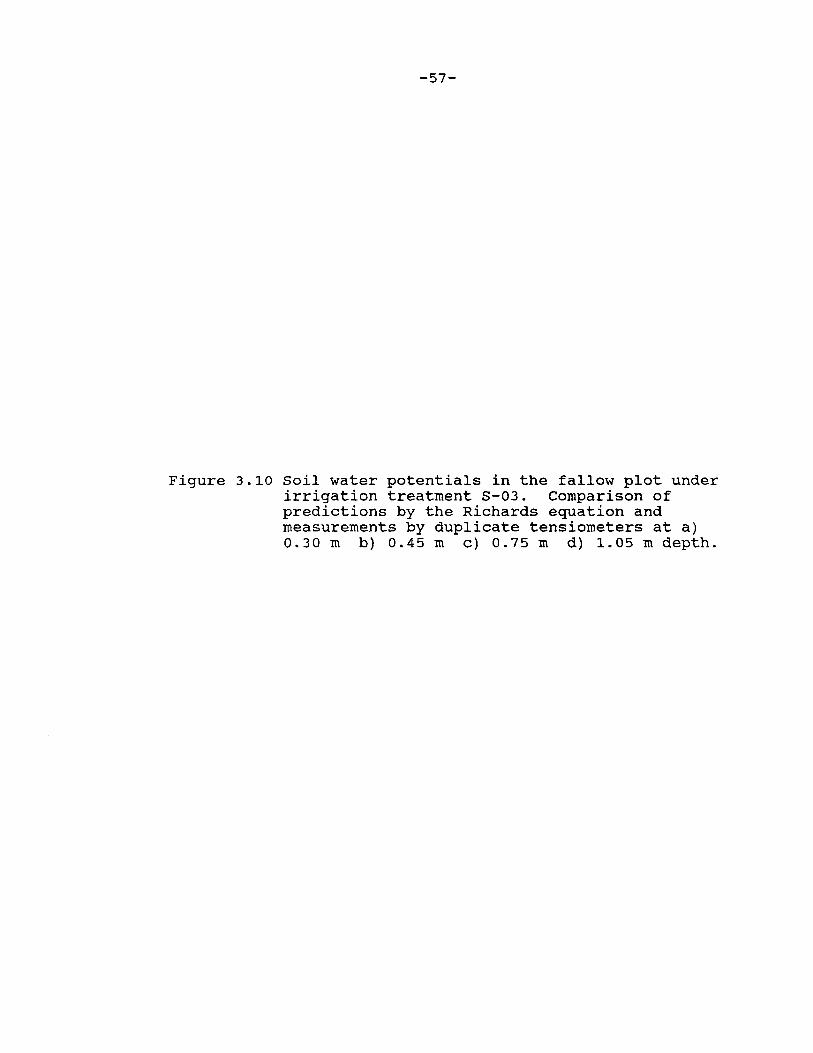
-57-

Figure 3.10 Soil water potentials in the fallow plot under irrigation treatment S-03. Comparison of predictions by the Richards equation and measurements by duplicate tensiometers at a) 0.30 m b) 0.45 m c) 0.75 m d) 1.05 m depth.

-C) .lil: --.., -.!! -C • -0 D. .. • -Cl 3=

0 (/J

-C) .lil: --.., -Cl -C • -0

D. .. • -Cl

3=

0 (/J

0-------------------, -5

-10

-15

-20

-25 Fallow Soll S-03,0.30 m

-o- Meas(0.30-1)

- Meas (0.30- 2)

- Pred (0.23) _30 ................. .....,rT'ft ........................................... ,.,.,., ....... 'TTTffT'rT'l"l ...... 'TTi

190 200 210 220 230 240

TIME (Julian Date)

Fallow Soll -25 S-03, 0.75 m

-o-- Meas(0.75-1)

- Meas (0.75 - 2)

- Pred (0.75)

250

-30 +.....-n ...... .....,rTY> ........................................... ,.,.,., ............ 'ffT' ............ -rrt

190 200 210 220 230 240 250

TIME (Julian Date)

.!! -C ., -0 D. .. ., -Cl

3=

= 0 (/J

-C, .lil: ..._ -, -.!! -C ., -0 D. .. ., -Cl 3=

= 0 (/J

-20

-25 Fallow Soll S-03, 0.45 m

-o-- Meas (0.45 - 1)

-+- Meas (0.45- 2)

- Pred (0.38)

- Pred (0.53)

-30 +-,,...... .................................... _... ............ __ ........... __ ...... _....,...,....-1

190

-5

-10

-15

-20

-25

200 210 220 230 240

TIME (Jullan Date)

Fallow Soll S-03, 1.05 m

Meas(l.05-1)

Meas (1.05 - 2)

- Pred (1.05)

250

-30 ;...,..,.......,..,.., ...... ,,..,, ......................................................................... ~ 190 200 210 220 230 240 250

TIME (Julian Date)

I Ul 0:,

I

-59-

Figure 3.11 comparison of measured soil water contents in the plots planted to corn with predictions by the Richards equation (R) and the Tipping Bucket routine (T) for Day 182 under four irrigation treatments corresponding to a) 1.6 b) 1.0 c) 0.6 and d) 0.3 potential evapotranspiration (PET).

-0.50

e ......

= -1.00 D. ., a

-1.50


a

Planted (1 .6 PET} Day 182 01 July 87

-- Predicted (R)

-- Predicted (T}

- Measured

t -2.oo-1-..------------..-.-.-............. ----...... .......1

-0.50

e ......

= -1.00 D. ., a

C

0.15 0.20 0.25 0.30 0.35


Planted (0.6 PET) Day 182 01 July87

-1.50 ---o-- Predicted (R)

-- Predicted (T)

-- Measured

0.40

-2.00 ......................................................... ,-r ....... -.-.............. -.-....... _.... ....... ~

0.15 0.20 0.25 0.30 0.35 0.40

-0.50

...... E ......

= -1.00 Q. ., a

-1.50

-0.50

e ......

= -1.00 D. ., a


b

Planted (1.0 PET) Day 182 01 July 87

-o- Predicted (R)

---.....- Predicted (T)

-- Measured

0.15 0.20 0.25 0.30 0.35


d

Planted (0.3 PET) Dey 182 01 July 87

-1.50 --o- Predicted (R)

- Predicted (T)

-- Measured

0.40

-2.00 ....... -.-........................................................................ -.-_.... ....... ,...,.....-1

0.15 0.20 0.25 0.30 0.35 0.40

I 0\ 0 I

-61-

Figure 3.12 Comparison of measured soil water contents in the plots planted to corn with predictions by the Richards equation and the Tipping Bucket routine for Day 225 under four irrigation treatments corresponding to a) 1.6 b) 1.0 c) 0.6 and d) 0.3 potential evapotranspiration (PET).

-0.50

'? .....


a

Planted (1.6 PET) Day225 13August87

= -1.00 a.

_i • C

'? ..... .r. -a. • C

-1.50 ·-- Predicted (R)

--.- Predicted (1)

- Measured

-2.00 -+-,..,...._,.......,,....._... ........................ _,. ........ ,.........._ ...... ,.._ ...... ._.....a

-0.50

-1.00

-1.50

0.15 0.20 0.25 0.30 0.35


C

Planted (0.6 PEl) Day 225 13August87

--o--· Predicted (R)

-- Predicted (1)

-- Measured

0.40

-2.00 -+-,..,.._,...,..,,...,....,_...,..,......__.. .................................................. ._.....a 0.15 0.20 0.25 0.30 0.35 0.40

-0.50 -E ..... = -1.00 a. • C

b


Planted (1.0 PEl) Day225 13August87

-1.50 --o- Predicted (R)

'? ..... .r. -a. • C

-0.50

-1.00

-1.50

--..-- Predicted (1)

-- Measured

0.15 0.20 0.25 0.30 0.35


d

Planted (0.3 PET) Day 225 13 August87

--0- Predicted (R)

- Predicted (1)

-- Measured

0.15 0.20 0.25 0.30 0.35

0.40

0.40

I CJ'\ I\J I

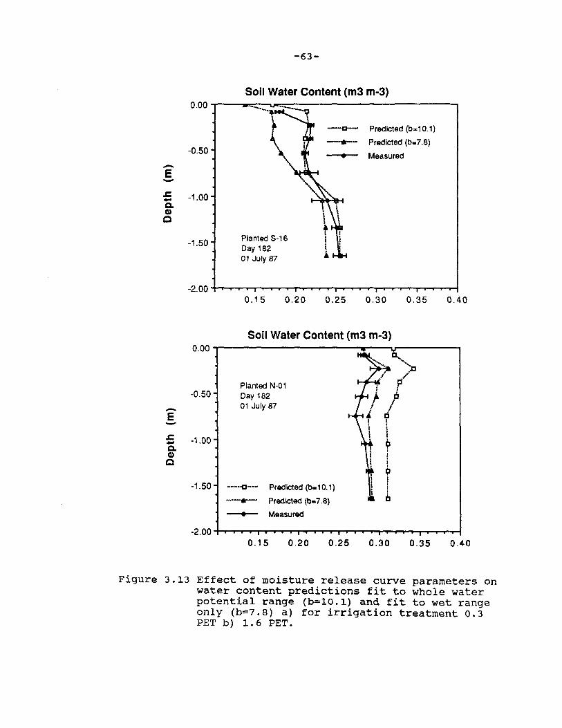
-0.50

-E -.J:. -1.00 -C. G)

C

-1.50

-2.00

0.00

-0.50

-E -.J:. -1.00 -C. G)

C

-1.50

-2.00

-63-


-o- Predicted (b .. 10.1)

-.- Predicted (b-7.8)

Planted S-16 Day 182 01 July 87

0.15 0.20

Measured

0.25 0.30 0.35

Soil Water Content (m3 m-3)

o......'i:i ...

Planted N-01 d/ i

Day 182 i 01 July 87

'?

\ ~ i

i ........ O···- Predicted (b-10.1) 1 ... -... - Predicted (b-7.8)

Measured

0.15 0.20 0.25 0.30 0.35

0.40

0.40

Figure 3.13 Effect of moisture release curve parameters on water content predictions fit to whole water potential range (b=lO.l) and fit to wet range only (b=7.8) a) for irrigation treatment 0.3 PET b) 1. 6 PET.

-64-

down to -1500 J kg· 1 • The reverse is true for the dry

treatment (0.3 PET), where using the wet range parameters

leads to a overprediction of plant water uptake and a

resulting underprediction of soil water contents. On day

182, predictions by the Richards equation are within 2 - 3

volume percent of the field measured values.

Predictions of soil water potentials coincide

reasonably well with the measurements. The drying and

rewetting in treatment N-03 (Fig. 3.14) between day 200

and 230 is again reflected in the predictions similar to

the fallow case, although measured water potentials drop

somewhat faster and to a lower potential than the

predictions indicate. In the N-08 treatment (Fig. 3.15),

the course of soil water potentials is predicted very well

for the 0.75 and 1.05 m depths, but the dry out of the

surface soil is not reflected in the predictions. For the

driest treatment modelled (N-13) (Fig. 3.16), soil water

potentials drop below the tensiometer range about the same

time in both the predictions and the measurements. Again,

the drying of the surface soil is not modelled well.

The discrepancies in simulated versus measured soil

water potentials can be explained by several possible

factors. First, predicted soil water potentials are

extremely sensitive to the choice of the value for air

entry potential (AE in equation 1). Lowering the air

entry potential only slightly will lower predicted soil

water potentials. Given the described problems about the

-65-

Figure 3.14 Soil water potentials in the cropped plot under irrigation treatment N-03. Comparison of predictions by the Richards equation and measurements by duplicate tensiometers at a) 0.30 m b} 0.45 m c} 0.75 m d) 1.05 m depth.

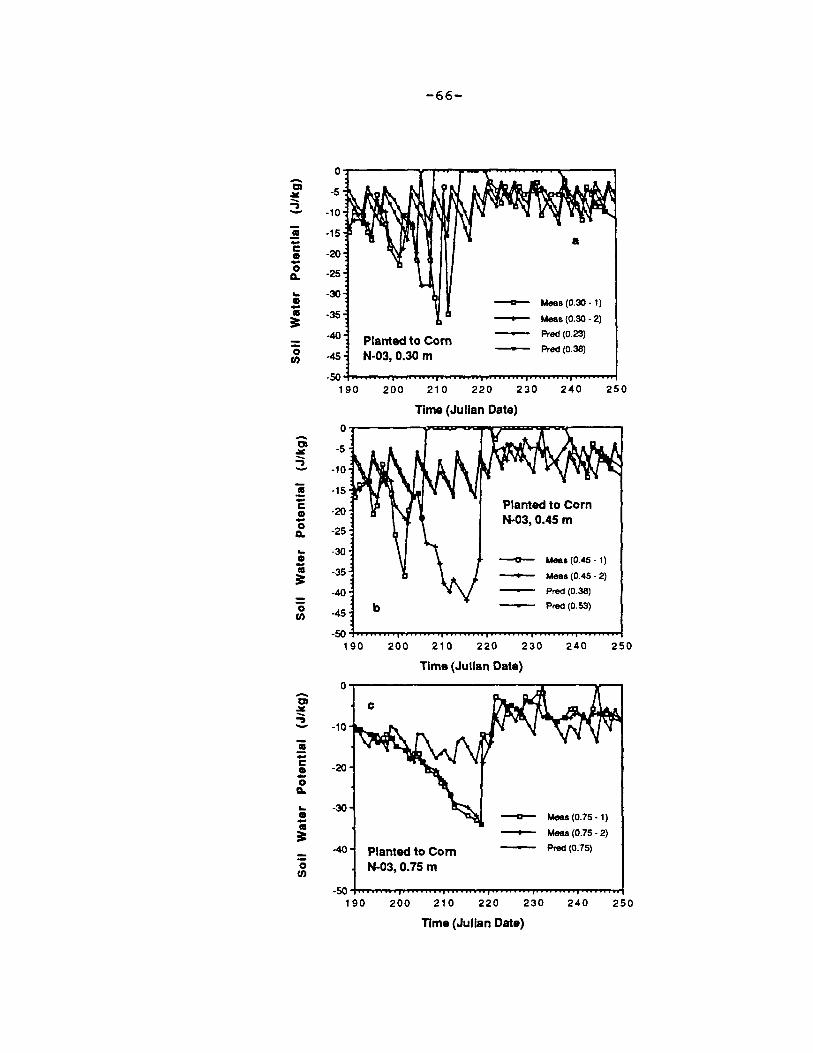
-~ -5 -., - -10

.!! -C • -0 Q. .. • -Ill 3

= 0 ti)

-15

-20

-25

-30

-35

-40

-45

-66-

Planted to Corn N-03, 0.30 m

a

--o- Meas (0.30 - 1)

- Meas (0.30 - 2}

- Pred (0.23)

- Pred (0.38)

.50,+.,...,.,.,..,.... ...................................................................................... ...i 190 200 210 220 230 240 250

-~ -5 ;:, - -10

.! -C • -0 Q. .. • -Ill 3

0 ti)

-15

-20

-25

-30

-35

-40

-45 b

Time (Julian Date)


--o- Meas (0.45 - 1}

- Meas (0.45 - 2)

Pred (0.38)

- Pred (0.53)

-so~ .............................................. ~""'"'"""' .................. _.. .......... ~ 190 200 210 220 230 240

Time (Julian Date)

-~ C -., - -10

~ -i -20 -0 Q. .. • -Ill 3

0 ti)

-30

-40 Planted to Com N-03, 0.75 m

--o- Meas (0.75 - 1)

- Meas(0.75-2)

- Pred (0.75)

250

-50*" ................................................................................ ~~~...a

190 200 210 220 230 240 250

Time (Julian Date)

-67-

Figure 3.15 Soil water potentials in the cropped plot under irrigation treatment N-08. Comparison of predictions by the Richards equation and measurements by duplicate tensiometers at a) 0.30 m b) 0.45 m c) 0.75 m d) 1.05 m depth.

..... Q .x -. .., .... .! -C • -0 G. .. • -al ~

= 0 U)

..... Q .x -. :?.

.! -C • -0 G. .. • -al ~

0 U)

-10

-20

-30

-40

-50

-60

-70

a

- Meas(0.30-1)

- Meas (0.30 - 2)

- Pred (0.23)

- Pred (0.38)


-80-t-r,,...,..,. ...... T"IT .............. ,.....,., .............................................................. ......1

160 170 180 190 200 210

Time (Julian Date)

o~-------------------. -10

-20

-30

-40

-50

-60

-70 Planted to Corn N-08,0.75 m

- Meas(0.75-1)

- Meas (0.75- 2)

Pred(0.75)

-so+., ............ T\"T .......................... ..-rr ....................................................... .......! 160 170 180 190 200 210

Time (Jullan Date)

..... Q .x -. .., .... al -C • -0

G. .. • -al ~

0 U)

..... Q .x .._ .., .... al -C • -0 G. .. • -al ~

0 U)

-10

-20

b -30

-40

-50

-60

-70

- Meas (0.45)

-..- Pred (0.38)

- Pred (0.53)


-so+., ...... ..-rrT\"T ............. ,.....'l"TT ...................................................... --1 160

-40

-50

-60

-70

170 180 190 200

Time (Julian Date)


- Meas(1.05-1) - Meas(1.05-2)

- Pred(1.05)

210

-80+-....... -r-......--.-......-..-................................................. ..-.............. --1 160 170 180 190 200 210 220 230 240 250

Time (Jullan Date)

I

°' co I

-69-

Figure 3.16 Soil water potentials in the cropped plot under irrigation treatment N-03. Comparison of predictions by the Richards equation and measurements by duplicate tensiometers at a) 0.30 m b) 0.45 m c) 0.75 m d) 1.05 m depth.

0 0 ..... .....

Planted to Com DI DI

.lil: a .lil: -20 N-13,0.45 m -- -20 ;; -, ----

.! -40 al -40 --C C

• -60 • -60 - -0 0

Q. Planted to Corn Q.

-80 N-13, 0.30 m .. -80 .. • • -- Meas (0.45 - 1) --al -100 - Pred(0.23) al -100 - Meas (0.45 - 2)

~ ~ - Pred (0.38) - Pred (0.38)

= -120 - MNs (O.~ - 1) -120 - Pred (0.53) 0 0 u, - MNs (O.~ - 1)

u,

-140 -140

160 170 180 190 200 210 160 170 180 190 200 210

Time (Julian Date) Time (Julian Date) I

0 0 ...J 0 ..... .....

DI C DI I .lil:

-20 .lil: d -- ;; -20 -, -- ......

.! -40 .! -40 - -C C

• -60 • -60 - -0 0 Q. -- Meas (0.75 - 1) Q.

-80 -80 Planted to Com .. - Meas (0.75 - 2) .. • • N-13, 1.05 m - - Pred (0.75) -al -100 al ~ ~ -100 -- Meas (1.05 - 1)

-120 Planted to Corn -120 - Mees (1.05 - 2) 0 N-13, 0.75 m

0 u, u, Pred (1.05)

-140 -140 160 170 180 190 200 210 160 170 180 190 200 210

Time (Julian Date) Time (Julian Date)

,

-71-

goodness of fit of the moisture release curve, predictions

compare well with the measurements. Second, assumptions

about rooting depth and densities will effect predicted

soil water potentials significantly. The fact, that

predictions do not coincide with the observed drying of

the soil surface could be the result of an underprediction

of roots in the surface soil compared to deeper layers.

This is supported by the faster predicted decrease in soil

water potentials at the 0.75 and 1.05 m depth, compared to

the measurements (Fig. 3.16). The lower than predicted

soil water contents in the soil surface could also be due

to an underprediction of available energy partitioned to

the soil surface for soil evaporation. The radiation

partitioning model used only partitions incoming solar

radiation. There is recent evidence that additional

energy can be available at the soil surface as a result of

heat convection within the canopy.

3.3.3 Water Budget Components

3.3.3.1 Fallow Soil

The predicted fluxes of applied water (soil

evaporation and drainage) is shown in Fig. 3.17 for the

fallow soil. Predictions of actual soil evaporation by

the Richards equation were consistently higher across all

irrigation treatments than the ones obtain from the

Tipping Bucket routine, probably due to the restriction of

-72-

Fallow Soil

500

-E 400

~ DR (R)

E - EV (R) )C :I LI. 300 a DR (T)

tV EV (T) -0 ~

200

100

0 -t-'T""""l'-,-,--~-..-.,....,,....... ....... ,....,._..,....'T""""I'._,..-,--~--~ 0 200 400 600 800 1 000 1200

Irrigation (mm)

Figure 3.17 Predicted total amounts of drainage below 1.20 m and predicted soil evaporation for fallow soil conditions over a range of irrigation water applications. a) predicted by the Richards equation (R) b) predicted by the Tipping Bucket routine (T).

-73-

evaporation to the uppermost layer in the Tipping Bucket

routine. Prediction by the Richards equation of soil

evaporation is very sensitive to the values chosen for the

soil hydraulic parameters affecting unsaturated hydraulic

conductivity.

Fig. 3.18 shows comparisons between predicted water

flux densities below a depth of 1.20 m, which was the

maximum crop rooting depth measured in the field. Because

the Tipping Bucket routine redistributes water in the soil

profile in discrete increments, predicted soil water

fluxes across the 1.20 m depth are not continuous, as are

fluxes predicted by the Richards equation. In the Tipping

Bucket routine, water movement only occurs when there is

water input at the top node, a result of the assumption

about field-capacity in conjunction with the normally used

daily time step.

Total amounts of predicted drainage are higher using

the Tipping Bucket routine, due mainly to the difference

in predicted soil evaporation. Predicted soil evaporation

was much higher using the Richards equation. Actual soil

evaporation is restricted to the uppermost soil layer in

the Tipping Bucket procedure with no upward flow of water

from lower depths being allowed. This will tend to

underpredict soil evaporation under wet conditions in

comparison to predictions made using the Richards

equation, as is evident from Fig. 3.19. Under dry

conditions differences in predicted values between the two

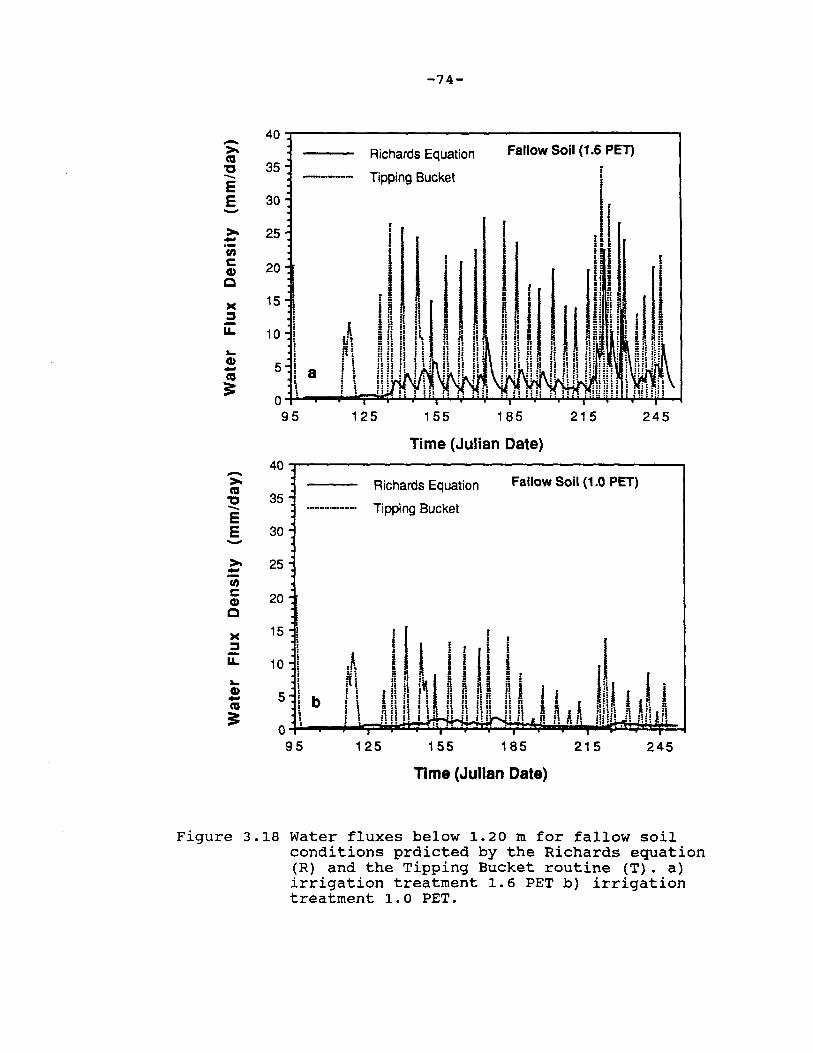
->, ca ,:, -E E ->, -en C G)

C

>< :::, -LL.

... G) -ca :=

->, ca ,:, -E E -

35

30

25

20

15

10

5

35

30

~ 25 en ; 20 C

>< :::, -LL.

... G) -ca :=

15

10

5 b

-74-

Richards Equation

Tipping Bucket

125 155

Fallow Soil (1.6 PET)

I

185 215

Time (Julian Date)

Richards Equation

Tipping Bucket

Fallow Soil (1.0 PET)

245

1 25 155 185 215 245

Time (Julian Date)

Figure 3.18 Water fluxes below 1.20 m for fallow soil conditions prdicted by the Richards equation (R) and the Tipping Bucket routine (T). a) irrigation treatment 1.6 PET b) irrigation treatment 1.0 PET.

->-"' "D -E E ->---,n C CD Q

,c :::, -u..

->-"' "D -E E ->--,n C Cl)

Q

,c :::, -u.. .. CD -"' ;:

-75-

6---------------------D

-+-5

• 4

3

2

Potential Soil Evaporation

Richards Equation

Tipping Bucket Fallow Soil (1.0 PEn

a

0 +..'-T-r ........ ~l'--T-r-T"" ............ 'T""l"......,. ...................... ,......,...,....T'"'l""T""l'"T""l'"......,. ............ -1

145 150 155 160 165 170 175 180 185

Time (Julian Date)

6----------------------D b

--.. + .. -

Potential Soil Evaporation

Richards Equation 5

• Tipping Bucket Fallow Soil (0.3 PEn

4

3 \ 2 \ 1 '.-+ 0 ..... "r-T" ....... l""'f'-l ....................... 'T"¥' .............. "T"'I'~ .............................. ,,,,.....,.~

145 150 155 160 165 170 175 180 185

Time (Julian Date)

Figure 3.19 Soil evaporation predicted by the Richards equation (R) and the Tipping Bucket routine (T) for fallow soil conditions. a) for irrigation treatments 1.0 PET b) 0.3 PET.

-76-

methods become smaller, due to the decrease in unsaturated

hydraulic conductivity upon drying and the concomitant

reduction of flow to the evaporating surface predicted by

the Richards equation. The predictions of actual soil

evaporation by the Richards equation are sensitive to

changes in air entry potential. A more negative air entry

potential will increase unsaturated hydraulic conductivity

at a given water potential, thus maintaining first-stage

soil evaporation for a longer time.

The predicted total amount of water present in the

upper 1.80 m of the soil profile is shown in Fig. 3.20 for

the four irrigation treatments in comparison with the

measured data. Good agreement is obtained between the

Richards equation and measured data for all but the excess

water (1.6 PET) treatment. A difference of 20 mm of total

water in the soil profile (1.80 m) corresponds to only

0.01 m3 m· 3 difference in average water content throughout

the profile. The predictions of total profile water by

the Tipping Bucket routine oscillate around the value

corresponding to field capacity, without reflecting well

changes in storage or continued drying as reflected in the

predictions by the Richards equation.


Total amounts of predicted actual transpiration over

the whole range of irrigation water treatments are very

similar as predicted by the potential-driven water uptake

-77-

Figure 3.20 Total amounts of water contained in the 1.80 m fallow soil profile as measured and as predicted by the Richards equation and the Tipping Bucket procedure. For irrigation treatments a) 1.6 PET b) 1.0 PET c) 0.6 PET and d) 0.3 PET.

.... 625 Richards Equation Fallow Soll (1.6 PET) - 625

Richards Equation Fallow Soll (1.0 PET)

E Tipping Bucket E Tipping Bucket

0 • 0 • Measured CIO

CIO ... 575 ... 575 - --

E E

E E --... 525 ... 525

• • - -• • ~ ~

• 475 • 475

- -0 0 b ... a ...

425 425

95 125 155 185 215 245 95 1 25 155 185 215 245

Time (Julian Date) Time (Julian Date) I ...., CX> I

- 625 Richards Equation Fallow Soll (0.6 PET) .... 625

Richards Equation Fallow Soll (0.3 PET)

E Tipping Buckel E Tipping Bucket

0 • Measured 0 • Measured

CIO CIO

... 575 .... 575 - --

E E

E E --... 525 ... 525

• • --• • ~ ~

475 475

• • --0 0 ... ...

425 425

95 125 155 185 215 245 95 125 155 185 215 245


-79-

procedure {in conjunction with the Richards equation) and

the Tipping Bucket procedure {Fig. 3.21). The Richards

equation predicts higher amounts of soil evaporation, most

likely for the reasons discussed above. The differences

in predicted drainage and soil evaporation are almost

constant across the range of irrigation water amounts,

which would suggest that both representations predict

about the same relative change in fluxes. Fig. 3.22 shows

the predictions {Richards equation) of the partitioning of

potential ET between soil evaporation and transpiration

and the degree to which this demand can be met under the

well-watered (1.0 PET) and a deficit treatments (0.3 PET).

Irrigation started on Day 132, after which actual rates of

both transpiration and evaporation proceed at potential

rates for the well-watered treatment. The much lower LAI

developed under irrigation treatment 0.3 PET is an

indication of the plant's ability to avoid severe water

stress through an early reduction in leaf area. However,

starting 45 days after emergence, water stress in terms of

transpiration deficit is indicated.

Under cropped conditions, predictions of actual

transpiration increase with increasing amounts of water

applied up to an amount equivalent to potential

transpiration, but predictions by either method are very

similar over a range of irrigation water treatments.

Predictions of drainage below 1.20 mare very similar to

the predictions for the fallow soil.

-ao-

Planted to Corn

500

~ DR (R) -E 400 EV(R)

E - a DR (T) >< ::::, - 300 • TR (R) u.

- ~ TR (T) as -0 • EV (T) I- 200

100

0 ~ ........ ~=:;:a;;:::;..........,_......,_......,_,... ........ _......,--.-1 0 200 400 600 800 1000 1200

Irrigation (mm)

Figure 3.21 Predicted total amounts of drainage below 1.20 m (DR), predicted actual transpiration (TR) and predicted soil evaporation (EV) for cropped soil conditions over a range of irrigation water applications. a) predicted by the Richards equation (R) b) predicted by the Tipping Bucket routine (T).

ct 7 ..J

- 6 >,, ca 't, -E 5 E ->,, 4 = Cl)

C 3 Cl>

C

)(

2 -= LL

... 1 Cl> -ca 3:

0 95

ct 6 ..J

->,, 5 ca 't, e E 4 ->,,

= U) 3 C Cl> C

... Cl> -ca

2

-81-

1.0PET(N-11)

125 155 185 215 245

Time (Julian Date)

0.3 PET (S-16)

3: o ~ .......... ~~L.ll~w....---==~~-..:uw1&.1 95 125 155 185 215 245

Time (Julian Date)

·-

D

---·-······ 0

D

Figure 3.22 Partitioning of potential evapotranspiration as predicted by the Richards equation. a) under irrigation treatment 1.0 PET b) under irrigation treatment 0.3 PET.

PET

PEV

PB/

PTA

A1R

LAI

PET

PEV

PB/

PTA

ATR LAI

-82-

Predictions of the total amount of water in the

profile using either method are in good agreement with the

measurements for the excess irrigation treatment (1.6 PET)

(Fig. 3.23). For the well-watered treatment (1.0 PET)

predictions by the Richards equation deviate after Day

180, after which water uptake is under-predicted. This is

also obvious from Fig. 3.11 and 3.12, where predicted soil

water contents are compared to the measured ones. In the

deficit (0.3 PET) treatments, water uptake as predicted by

both the Richards equation and the Tipping Bucket routine

is similar and fits observations well. The under

prediction of water uptake by the Richards equation in the

well-watered treatment could be the result of advection,

which has been identified as an important factor in the

energy budget under Cerrado conditions (Luchiari, 1988).

This is supported by the comparison of Priestley-Taylor

predicted ET rates with 'Class A' pan measurements. The

drastic increase in evaporative demand after day 180

reflected in the pan data is not represented by Priestley

Taylor predictions. A higher value for the Priestley

Taylor coefficient would have to be used under these

circumstances (Luchiari, 1988).

Interception of precipitation or irrigation water

could have an effect on the water budget of the soil-plant

system. A value of 2.5 mm was reported as the maximum

interception capacity of a corn canopy (Sudar et al,.

1981) and used in the simulations. Including canopy

-83-

Figure 3.23 Total amounts of water contained in the 1.80 m soil profile planted to corn as measured and as predicted by the Richards equation and the Tipping Bucket procedure. For irrigation treatments a) 1.6 PET b) 1.0 PET c) 0.6 PET and d) 0.3 PET.

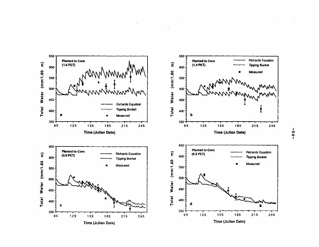
650 650

- Planted to Corn ..... Planted to Corn Richards Equation

E 600

(1.6 PET) E 600 (1.0 PET) Tipping Bucket

0 0 • Measured CC? CD .... 550 .... 550 -E e E E - 500 - 500 .. .. • • - -• 450 • ~ ~ 450

Richards Equation

• 400 Tipping Bucket iii - - 400 0 0 I- • • Measured I- b

350 350 95 125 155 185 215 245 95 125 155 185 215 245

I Time (Julian Date) Time (Julian Date) 0)

~

I

650 650

Planted to Corn - Planted to Corn Richards Equation - Richards Equation

E (0.6 PET) E (0.3 PET) 600 Tipping Bucket

600 Tipping Bucket 0 0 CD • Measured CC? • Measured .... 550 - 550 - e E E E - ......

500 500 .. .. • • - -• • 450 ~ 450 ~

111 • 400 - 400 -0 0 I- I- I

350 350

95 125 155 185 215 245 95 125 155 185 215 245


-85-

interception as a simulated process led to a reduction of

transpiration by the amount intercepted (60 mm) and

evaporated off the leaves, but did not affect predicted

drainage or soil evaporation significantly. Also, soil

water contents were barely affected by the inclusion of

interception.

3.4 SUMMARY AND CONCLUSIONS

Comparisons between the Richards equation and

capacity-type, water content based representations of soil

water flow have been limited (Da Silva and de Jong, 1986).

This is partly due to the difficulties encountered when

comparing two different simulation models that contain

other component processes besides the ones to be compared.

GAPS provides an e~vironment in which two alternative

representations can be compared without changing the other

component processes given that both modules provide the

needed output for the other procedures in use. Choosing

one of these two water flow models has clear effects on

the freedom of choice regarding other component parts,

e.g. a potential driven plant water uptake routine can not

be linked to the Tipping Bucket routine since the latter

does not provide needed estimates of soil water potentials

over time and space.

Both the Richards equation and the Tipping Bucket

water flow models were found to predict soil profile water

contents well, when compared to field measured data. Both

-86-

methods have their respective strengths and weaknesses.

The Richards equation performed better in predicting soil

water contents over the whole range of irrigation water

treatments and is better able to predict soil profile

water content distributions. Drainage fluxes predicted by

the Richards equation are continuous as opposed to the

more discrete flux events predicted by the Tipping Bucket

method. The soil evaporation component of the Tipping

Bucket routine would have to be made more complex,

possibly including upward flow, in order to simulate soil

evaporation better.

Capacity-type flow representations such as the Tipping

Bucket routine are used extensively in crop simulation

models due to their perceived conceptual simplicity and

computational efficiency. It is also often argued that

input parameters for the latter model are more easily

available than the parameters necessary to estimate water

content-water potential relationship needed for the

Richards equation. The Tipping Bucket water flow

procedure is sensitive to the value chosen for field

capacity water content. This was particularly obvious in

the simulations of fallow soil conditions. Given this

sensitivity, the choice of the appropriate soil water

potential for field capacity becomes crucial.

Clearly, the predictions of water contents and

potentials as well as predicted plant water uptake, using

the Richards equation and potential driven water uptake,

-87-

are highly sensitive to the parameters calculated for the

moisture release curve. This sensitivity does not always

become apparent, especially if only tested under a narrow

set of environmental conditions. The wide range of

irrigation water treatments used in this study made the

sensitivity of the predictions to moisture release

parameters under certain condition apparent.

Several soil properties specific for highly weathered

Oxisols have important implications for water flow

modeling. The soil moisture release curve of the Oxisol

studied in this research resembled a silt loam on the wet

end and a clay on the dry end. The power function used to

model the moisture release curve (Campbell, 1974, 1985)

does not appear to provide a good enough fit to moisture

release data for these Oxisols, when fitted over the whole

range of water potentials to -1500 J kg· 1 • If the

emphasis of the modeling effort is the prediction of water

flow and water contents under well irrigated conditions,

it is advisable to use parameters fitted to the wet range

(to -100 J kg· 1 ) only. Under irrigated conditions, the

soil would not reach water potentials of less than -100 J

k . 1 g . Ideally, a different function better describing he

unique behavior of this soil should be used.

Field saturated water contents never reach total

porosity in the field, and the percentage of total

porosity at field saturated water contents appears to be

much lower than the percentages assumed for temperate

-88-

soils. A knowledge of the soil water content at

saturation in the field is essential in order to predict

soil water contents correctly, using the Richards

equation. The effect of decreased total porosity due to

compaction and reflected in increased bulk densities does

not result in an equivalent decrease in saturated water

contents under field conditions.

Limited measurements on rooting depths and

distributions were available for this study. No

differences in rooting depth or density were assumed

between the different irrigation treatments. The

deviation of predicted from measured soil water potentials

in the dry treatments indicates that root water uptake was

underpredicted in the soil surface and overpredicted at

deeper soil depths. The occurrence of advective

conditions in the Cerrado was reported by Luchiari (1988)

and further evidence for the frequency of their occurrence

was evidenced in this experiment.

REFERENCES

Bouldin, D.R., s. Mughogho, D. J. Lathwell, and T. w. Scott. 1979. Nitrogen fixation by legumes in the tropics. Cornell Int. Agric. Mimeo 75. Cornell University, Ithaca NY.

Buttler, I. W. ands. J. Riha. 1987. General purpose simulation model of water flow in the soil-plantatmosphere continuum. Appl. Agr. Res. 2:230-234.

Buttler, I. w. ands. J. Riha. 1988. GAPS - A general purpose simulation model of the soil-plantatmosphere. User's manual (Draft). Cornell University, Ithaca, NY.

-89-

Campbell, G. s. 1974. A simple method for determining unsaturated conductivity from moisture retention data. Soil Sci. 117:311-314.

Campbell, G. s. 1985. Soil physics with BASIC: Transport models for soil-plant systems. NY Elsevier.

Da Silva, c. c. and E. de Jong. 1986. Comparison of two computer models for predicting soil water in a tropical monsoon climate. Agr. and Forest Meteorology 36:249-262.

EMBRAPA/CPAC. 1981. (in portuguese) Relatorio Tecnico Anual do Centro de Pesquisa Agropecuaria dos Cerrados 1979-1980. Planaltina-DF, Brazil.

EMBRAPA/CPAC. 1978. (in portuguese) Relatorio Tecnico Anual do Centro de Pesquisa Agropecuaria dos Cerrados 1976-1977. Planaltina-DF, Brazil.

Fisher, M. J., Charles-Edwards, D. A., and M. M. Ludlow. 1981. An analysis of the effects of repeated short term soil water deficits on stomatal conductance to carbon dioxide and leaf photosynthesis by the legume Macroptiliurn atropurpureurn cv. Siratro. Aust. J. Plant Physiol. 8:347-357.

Foth, H. D. 1962. Root and tap growth of corn. Agron J. 54:49-52.

Gardner, W.R. 1960. Dynamic aspects of water availability to plants. Soil Sci. 89:63-73.

Gardner, W.R. and C. F. Ehlig. 1962. Some observations on the movement of water to the plant. Agron.J. 54:453-456.

Garrido, W. c., Silva, E. M., and o. c. Souza. 1979. Water-use efficiency by wheat varieties in the cerrado soil of Brazil. In: Soil physical properties and crop production in the tropics (eds. R. Lal and D.G. Greenland), Wiley, New York.

Gee, G. w. and J. W. Bauder. 1985. Particle-size analysis. In: Methods of soil analysis. Part 1 -Physical and mineralogical methods. A. Klute (ed.). 2nd edition, ASA, MAdison, WI.

Gonzales-Erice, E., Karnprath, E. J., Naderman, G. c., and w. V. Soares. 1979. Effect of depth of lime incorporation on the growth of corn on an Oxisol of central Brazil. Soil Sci. Soc. Arn. J. 43:1155-1158.

-90-

Goodwin, J. B., Garacorry, F. L., Espinoza, W., Sans, L. M., and L. J. Youngdahl. 1982. Modelling soil-waterplant-relationships in the Cerrado soils of Brazil: The case of maize. Agric. Systems 8:115-127.

Grove, T. L., K. D. Ritchey, and G. c. Naderman, Jr. 1979. Nitrogen fertilization of maize on an oxisol of the Cerrado of Brazil. Agronomy J. 72:261-265.

Hanks, R. J., J. Keller, V. P. Rasmussen, and G. D. Wilson. 1976. Line source sprinkler for continuous variable irrigation-crop production studies. Soil Sci. Soc. Am. Proc. 40:426-429.

Jones, c. A. and J. R. Kiniry. (eds). 1986. CERES-Maize. A simulation model of maize growth and development. Texas A&M University Press, College Station. 194 pp.

Klute, A. and C. Dirksen. 1985. Hydraulic conductivity and diffusivity: Laboratory methods. In: Methods of soil analysis. Part 1 - Physical and mineralogical methods. A. Klute (ed.). 2nd edition, ASA, Madison, WI.

Lobato, E. and D. K. Ritchey. 1979. Improvement and fertilization of the savanna in Brazil. Tropical agriculture research series 15.

Luchiari, A. 1988. Measurements and predictions of evaporation rates from irrigated wheat in the Cerrados region of central Brazil. Ph.D. thesis, Cornell University, Ithaca, NY.

Macedo, J. and R. B. Bryant. 1987. Morphology, mineralogy, and genesis of a hydrosequence of Oxisols in Brazil. Soil Sci. Soc. Am. J. 51:690-698.

Norman, J. N., and G. s. Campbell. 1983. Application of a plant-environmental model to problems in irrigation. Adv. Irrig. 2:155-188.

Priestley, C.H. B. and B. J. Taylor. 1972. On the assessment of surface heat flux evaporation using large-scale parameters. Mon. Weather Rev. 100:81-92.

Pruntel, J. 1975. water availability and soil suitability for irrigation water impoundments in the Federal District of Brazil. M.S. thesis. Cornell University. Ithaca, NY.

-91-

Riha, S. J. and G. s. Campbell. 1985. fluxes in Douglas-fir plantations. 15:701-707.

Estimating water Can. J. For. Res.

Ritchey, K. D. 1979. Potassium fertility in oxisols and ultisols of the humid tropics. Cornell Intern. Agr. Bulletin 37. Cornell University, Ithaca, NY.

Ritchey, K. D. 1982. Calcium deficiency in clayey Bhorizons of savanna oxisols. Soil Sci. 133:378-382.

Ritchie, J. T. 1972. Model for predicting evaporation from a row crop with incomplete cover. Water Resources Res. 8:1204-1213.

Ritchie, J. T., J. R. Kining, C. A. Jones and P. T. Dyke. 1986. Model Inputs. In: CERES-Maize. A Simulation Model of Maize Growth and Development. c. A. Jones and J. R. Kiniry (Eds). Texas A&M University Press, College Station. 194 pp.

SAS Institute Inc., 1985. SAS user's guide: Basics. SAS Institute Inc., Cary, NC.

Stockle, c., and G. s. Campbell. 1985. A simulation model for predicting effect of water stress on yield: an example using corn. Adv. in Irrigation 3:283-323.

Sudar, R. A., K. E. Saxton, and R. G. Spomer. 1981. A predictive model of water stress in corn and soybeans. Transactions of the ASAE 24:97-102

Van Wambeke, A., Hastings, P., and M. Tolomeo. 1986. Newhall Simulation Model. Department of Agronomy, Cornell University, Ithaca, NY.

Wagenet, R. J. and J. L. Hutson. 1986. Predicting the fate of nonvolatile pesticides in the unsaturated zone. J. Environ. Qual. 15:315-322.

Wolf, J.M. 1975. Water constraints to corn production in Central Brazil. Unpublished Ph.D. Thesis, Cornell University.

Chapter IV

PREDICTING CORN GROWTH AND YIELDS

UNDER VARIABLE WATER INPUTS

4.1 INTRODUCTION

The specific soil and climatic conditions of the

Cerrado region in Brazil make an understanding of plant

water relations a prerequisite for a wide range of

agricultural research objectives. Extremely low water

holding capacities of the predominant soil orders (Oxisols

and Ultisols) in combination with frequently occurring

drought periods (veranicos} during the wet season

(September to March} can cause water stress and yield

reductions in crops (Wolf, 1975; Goodwin, et al. 1982).

During the occurrence of a one to two week drought, the

survival of the crop is largely determined by the amount

of stored water that is accessible to the root system.

The highly weathered acid soils restrict rooting depth to

the zone where Al-toxicity and Ca-deficiency have been

corrected by soil amendments (Ritchey, 1982). Deep

incorporation of lime was shown to effectively reduce

water stress and avoid concomitant reductions in yield in

this region (Bandy, 1976). When water stress equivalent

to a typical veranico was imposed on a corn crop, leaf

water potentials were shown to drop less and recover

earlier in the day in the deep lime treatment compared to

treatment receiving no lime amendment. Grain yields in

-92-

-93-

these experiments were reduced 42% in the no-lime

treatment compared to 8% in the limed treatment.

Increased rooting depth was suggested as the most likely

mechanism to account for the drought avoidance.

Components of a corn growth simulation model

previously implemented by Stockle and Campbell (1985) was

incorporated into the General Purpose Simulation Model

GAPS (Buttler and Riha, 1987) and its applicability to

Cerrado conditions tested. A crop growth component model

that can respond to climate and soil water status is

necessary for predicting crop response over a broad

region, as well as a precursor to analysis of other

production constraints, such as nitrogen. The objective

of this research was to determine the effect of limiting

water on corn growth and yield, in order to be able to

predict the effects of varying inputs on corn yield and

water fluxes under a range of soil fertility and climatic

conditions found in the savanna regions of the tropics.

In chapter III, water flow components of the GAPS

model were shown to satisfactorily simulate soil water

fluxes and budgets under Cerrado conditions under bare

soil as well as cropped conditions. For the simulations

of cropped conditions, functions fitted to measured

experimental data were used to provide leaf area index

over time for different irrigation treatments. In this

chapter, growth of the crop, including simulation of leaf

area index, is predicted through simulation of

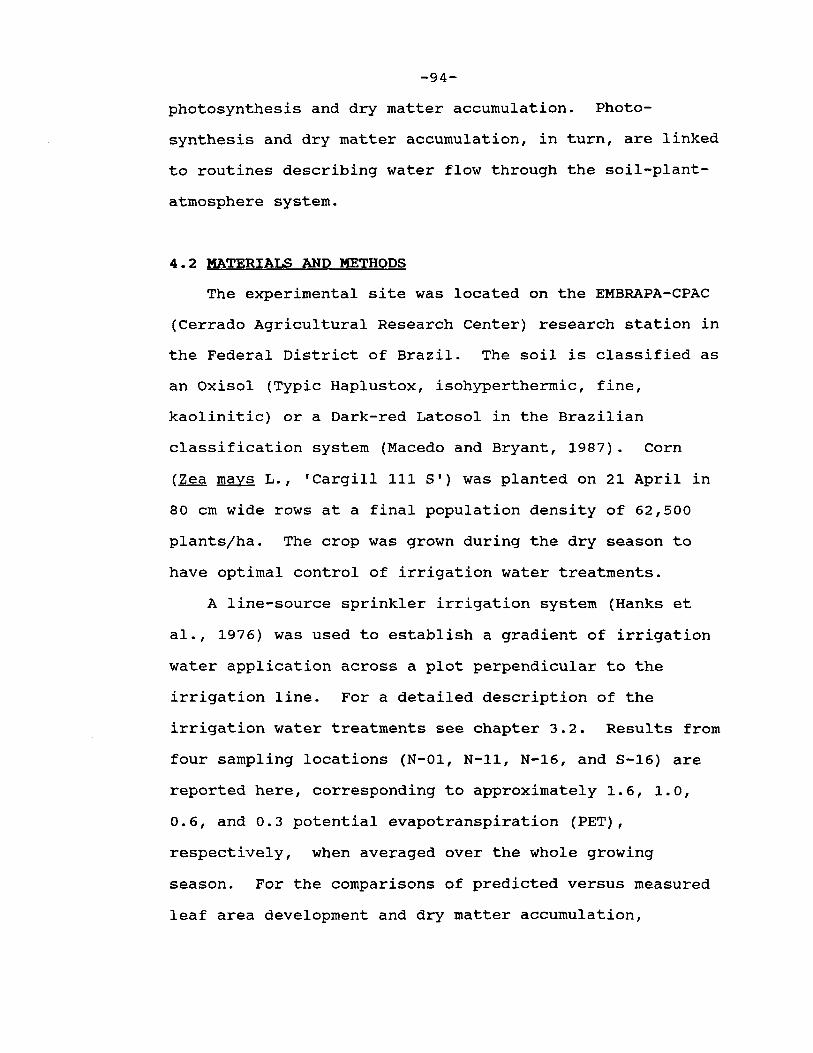
-94-

photosynthesis and dry matter accumulation. Photo

synthesis and dry matter accumulation, in turn, are linked

to routines describing water flow through the soil-plant

atmosphere system.

4.2 MATERIALS AND METHODS

The experimental site was located on the EMBRAPA-CPAC

(Cerrado Agricultural Research Center) research station in

the Federal District of Brazil. The soil is classified as

an Oxisol (Typic Haplustox, isohyperthermic, fine,

kaolinitic) or a Dark-red Latosol in the Brazilian

classification system (Macedo and Bryant, 1987). Corn

(Zea mays L., 'Cargill 111 S'} was planted on 21 April in

80 cm wide rows at a final population density of 62,500

plants/ha. The crop was grown during the dry season to

have optimal control of irrigation water treatments.

A line-source sprinkler irrigation system (Hanks et

al., 1976) was used to establish a gradient of irrigation

water application across a plot perpendicular to the

irrigation line. For a detailed description of the

irrigation water treatments see chapter 3.2. Results from

four sampling locations (N-01, N-11, N-16, and S-16) are

reported here, corresponding to approximately 1.6, 1.0,

0.6, and 0.3 potential evapotranspiration (PET),

respectively, when averaged over the whole growing

season. For the comparisons of predicted versus measured

leaf area development and dry matter accumulation,

-95-

measured data from several rows was pooled according to

amounts of irrigation water received, where appropriate.

'A4' refers to a pooling of irrigation treatments N-01, s-

01, and N-06, and 'A3' to a pooling of N-11 and S-06 (see

also Fig. 3.1 b).

Sequential harvests of the above-ground portion of the

corn plants were conducted weekly for the first five weeks

starting 31 days after emergence and then biweekly for a

total of 10 sampling dates. Five plants (one consecutive

meter) were sampled per row, corresponding to a specific

irrigation treatment. Green and dry leaf area were

determined with a leaf area meter. Dry weight of stalks,

green leaves, flag leaf, dry leaves, tassel, and spikes

was determined separately and are summed as total above

ground dry weight. For the final harvest on 22/23

September, all corn rows not previously used for

sequential harvests were used. The six central meters of

every row were harvested, and total dry matter and grain

yield were determined.

4.3 SIMULATION OF CROP GROWTH

Components of a corn growth simulation model (Stockle

and Campbell, 1985) were recoded and translated into

PASCAL, in some instances revised, and incorporated into

the General Purpose Simulation Model GAPS (Buttler and

Riha, 1987). Photosynthesis is calculated on the basis

of photosynthetically active radiation (PAR) intercepted

-96-

by the canopy using an equation proposed by Norman (1982)

to estimate PAR, an equation to estimate the canopy

extinction coefficient as given by Campbell (1977) and

equations proposed by Hesketh and Baker (1967) for

relating photosynthetic rate to intercepted PAR. The

estimate of photosynthetic rate incorporates the effects

of temperature assuming leaf temperature equal to air

temperature.

Growth is directly related to photosynthesis by using

an average conversion factor of 0.40 as suggested by

Monteith (1981). This conversion factor was not varied as

done by Stockle and Campbell (1985). The estimate of

photosynthetic rate is used to calculate a no-stress

canopy resistance for vapor transport. The concept of

critical leaf water potential (Fisher et al, 1981; Turner,

1974) is used to calculate actual transpiration. It is

assumed that canopy resistance responds little to a

lowering in leaf water potential until a critical value is

reached, at which resistance increases rapidly over a

relatively narrow range. A critical leaf water potential

of -1.4 MPa was used. Leaf water potential is calculated

from hourly simulation of root water potential.

Knowing the canopy resistance as a function of leaf

water potential, the reduction in potential transpiration

can be calculated. The photosynthetic rate previously

calculated for the non-stressed condition is reduced

proportionally to the decrease in transpiration rate.

-97-

Photosynthetic rates are calculated on an hourly time

step, summed for one day and converted into dry matter.

The daily accumulated dry matter is partitioned into top

and root dry matter using data presented by Foth (1962).

Rooting depth is empirically related to root dry matter

(Acevedo, 1975). No correction for water stress on

partitioning as included in Stoeckle and Campbell (1985)

was used for these simulations. Table 4.1 lists

differences in processes and parameter values between

Stockle and Campbell's model and this particular

implementation.

A function for accumulated thermal time (FT) was used

to separate corn phenological stages into vegetative (FT<

33), pollination (33<= FT <40), and grain filling (40 <=

FT< 49) stages (Coelho et al. 1980).

To convert above-ground dry matter into leaf area

during the vegetative phase the relationships originally

included in Stockle and Campbell's model, and based on

independent data sets of Acevedo (1975) were used. During

pollination, leaf area is reduced as a function of

attained leaf area index and thermal time (Dale et al.,

1980) with a correction for water stress as proposed by

Stockle and Campbell (1985). The more water stress has

been accumulated during the vegetative phase, the more

rapid will the decline of leaf area occur. After the end

of the pollination phase, leaf area declines as a function

of time (Dale et al., 1980).

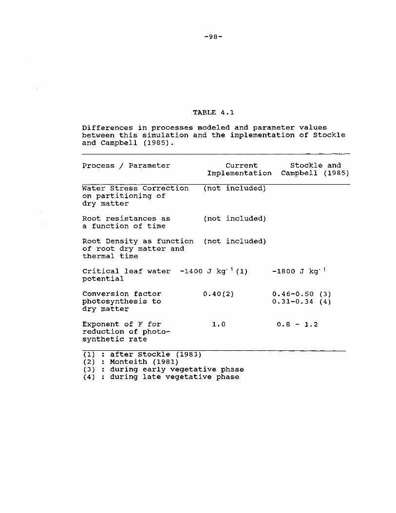
-98-

TABLE 4.1

Differences in processes modeled and parameter values between this simulation and the implementation of Stockle and Campbell (1985).

Process/ Parameter Current Implementation

Water Stress Correction (not included) on partitioning of dry matter

Root resistances as (not included) a function of time

Root Density as function (not included) of root dry matter and thermal time

critical leaf water -1400 J kg· 1 (1) potential

Conversion factor 0.40(2) photosynthesis to dry matter

Exponent of F for 1.0 reduction of photo-synthetic rate

( 1) : (2) (3) (4)

after stockle (1983) Monteith (1981) during early vegetative phase during late vegetative phase

Stockle and Campbell (1985)

-1800 J kg" 1

0.46-0.50 (3) 0.31-0.34 (4)

0.8 - 1.2

-99-

4.4 RESULTS AND DISCUSSION

4.4.1 Effect of Amount of Irrigation Water on Dry

Matter Accumulation And Leaf Area Development

4.4.1.1 Sequential Harvests

Leaf area for the 1.0 PET (100 % of potential

evapotranspiration) and the 0.6 PET (60 % of potential

evapotranspiration) irrigation treatments developed

similarly until day 180, when they reached a peak leaf

area index (LAI) of about 5.0 (Fig. 4.1 a). After day

180, which coincides with time of tasseling, leaf area in

treatment 0.6 PET decreased more rapidly than in the well

watered (1.0 PET) treatment, indicating the effect of

water stress. The 0.3 PET treatment exhibits a pronounced

reduction in leaf area development from the beginning.

Leaf area peaked around day 180 at a LAI of about 2.5,

before starting to decline. Interestingly, a decrease in

initial rate of leaf area development and dry matter

accumulation was observed in treatment 1.6 PET (Fig.4.1

a). Later in the season, treatment 1.6 PET was able to

maintain a higher leaf area for a longer time than

treatment 1.0 PET. This resulted in continued dry matter

accumulation after day 220, when dry matter accumulation

rates in the other treatments had already slowed (Fig. 4.1

b). Treatment 1.6 PET eventually reached the highest dry

matter and also the highest grain yield.

The leaf area ratio (LAR), the dry weight of leaves as

a fraction of total above-ground dry matter decreased with

-100-

6 a - N-01

5 N-11

• N-16

S-16 4

< 3 ..J

2

1

0 140 170 200 230 260

Time (Julian Date) 3000

b

- 2500 N ~ N-01

I

E N-11

2000 a N-16 C, - S-16 ... I Q) 1500 --as :E

1000 ! >-... C i

500

0 140 170 200 230 260

Time (Julian Date)

Figure 4.1 Crop growth under different irrigation treatments: N-01 (1.6 PET), N-11 (1.0 PET}, N-216 (0.6 PET) and S-16 (0.3 PET). a) Leaf area index b) total above-ground dry matter. Error bars represent +l u.

-101-

time (Fig. 4.2), and was not statistically different

between irrigation treatments.

4.4.1.2 Final Harvest

The increase in above-ground dry matter accumulation

was nearly linear with the amount of irrigation water

applied to an amount equivalent to potential

evapotranspiration (641 nun) (Fig. 4.3 a). After that,

final dry matter levelled off, although considerable

variability in final dry matter is exhibited at high water

levels. Final dry matter yields estimated using the

regression equation fit to the data in Fig 4.3 a are 26

Mg/ha at 1020 mm of water applied (1.6 PET) compared to 21

Mg/ha at an irrigation corresponding to 1.0 PET.

Increase in grain yields with increased amounts of

irrigation water applied were nearly linear over the whole

range. Grain yields reached 9.2 Mg/ha at 1020 mm of

irrigation water applied compared to 6.0 Mg/ha at an

irrigation amount corresponding to PET (Fig. 4.3 b).

Grain yield was clearly more severely effected by water

deficit than total above-ground dry matter as shown by a

rapid decrease in harvest index at irrigation amounts less

than PET (Fig. 4.3 c). At irrigation levels above PET the

harvest index leveled off around values of 0.33 to 0.34.

-102-

Leaf Area Ratio

30

Ill A1

25 - • A2 .

a A3

20 - I • • A4 - Ill C) a .:ii: -CN a E • - 15 - • cc • <C I ....J • Ill

10 - • a

• Iii

5- • a I

0 I I I

20 40 60 80 100

Days after emergence

Figure 4.2 Leaf area ratios (leaf area/total above-ground dry weight) for different irrigation treatments: A4 (N-01, N-06, S-01), A3 (N-11, S-06), A2 (N-16, S-11), and Al (S-16).

-103-

Figure 4.3 Yield as a function of applied irrigation water (PET= 641 mm): a) final above-ground dry matter, b) grain yield and c) harvest index.

-104-

40

a OM• - 1.527 + 0.049 IRR- 2.15ne-5 IRR·2 35 R•2.0.922

30 • • - •• • • s: 25 Q ::::& - 20

~ Q 15 • ...

10

5

0 0 200 400 600 800 1000 1200

Irrigation Water Applied (mm)

15 GY. - 1.457 + 0.0136 IRR - 3.098-6 IRR•2

R•2. 0.896 - b • Ill s: • Cl ::::& 10 -~ .! > C 5 Ill .. C,

0 0 200 400 600 800 1000 1200


0.5 HI. - O.D18 + 8.096&-4 IRR - 4.53e-7 IRR•2

R•2.o.686 C • 0.4 •

)C • mP • • "a •• a 1111 C 0.3 • •• • -• II • > 0.2 ... • :c •

0.1

0.0 0 200 400 600 800 1000 1200


4.4.2

-105-

Comparison of Measured and Predicted Crop

Growth and Development

Model predictions of dry matter accumulation and leaf

area for the 1.6 PET and 1.0 PET treatments are identical,

since neither treatment experienced any water stress that

would have resulted in a reduction of simulated growth

rates. Predictions of accumulated top dry matter for

treatment 1.0 PET correspond very well with measured data

(Fig 4.4). The course of dry matter accumulation until

day 205, which corresponds to about 15 days after

tasseling, is very well simulated (Fig. 4.4 b). The end

of further dry matter accumulation in the model is

triggered when maturity (FT> 49) is reached. Leaf area

after this date starts declining rapidly as a function of

time (Dale, et al., 1980) and accumulated stress (Stockle

and Campbell, 1985). Although the time course of leaf

area decline is simulated well, final dry matter is being

overpredicted.

The lower measured dry matter accumulation in

treatment 1.6 PET (Fig. 4.5 b) as compared to the

predictions as well as the measured dry matter

accumulation in 1.0 PET could be the result of early

leaching losses of applied fertilizer nitrogen below the

root zone of the young corn plant, which might have

delayed initial growth.

The time course of leaf area development corresponds

to measured data (Fig. 4.5 a), although the initial rate

-106-

6

a N-11 5

4

<( 3 ..J

I 2

Predicted 1 • Mean A3

II N-11

0 105 135 165 195 225 255

Time (Julian Date)

3

b N-11

-N I

E C, 2 Predicted Ill

.=.::: Ill Measured -... G) --cu

::E 1 >,. ... C

0 .J-...-...,m~cm::;_..--..--.,..--......-..---......----.........I 105 135 165 195 225 255

Time (Julian Date)

Figure 4.4 Comparison of measured and predicted crop growth for irrigation treatment N-11 (1.0 PET): a) leaf area and b) accumulated dry matter. Means of leaf area for plants in group A3 (N-11, S-06) +1 u. Also, the measured value for N-11 is included.

-107-

6 a N-01

5

4

ct 3 ..J

2

Predicted 1 II Measured

0 105 135 165 195 225 255

Time (Julian Date)

3

b N-01

-N I

E Predicted • 2 C') • Measured .lll:: -...

Cl) --cu :i:

>-... C

0 ~ ... -.~~~~--------....-----------l 105 135 165 195 225 255

Time (Julian Date)

Figure 4.5 Comparison of measured and predicted crop growth for irrigation treatment N-01 (1.6 PET): a) leaf area and b) accumulated dry matter. Means of leaf area for plants in group A4 (N-01, N-06, S-06) +1 U. Also, the measured value for N-01 is included.

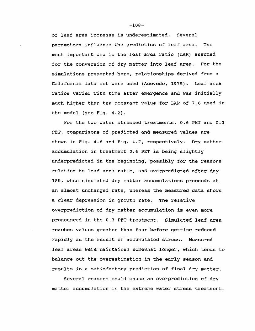
-108-

of leaf area increase is underestimated. Several

parameters influence the prediction of leaf area. The

most important one is the leaf area ratio (LAR) assumed

for the conversion of dry matter into leaf area. For the

simulations presented here, relationships derived from a

California data set were used (Acevedo, 1975). Leaf area

ratios varied with time after emergence and was initially

much higher than the constant value for LAR of 7.6 used in

the model (see Fig. 4.2).

For the two water stressed treatments, 0.6 PET and 0.3

PET, comparisons of predicted and measured values are

shown in Fig. 4.6 and Fig. 4.7, respectively. Dry matter

accumulation in treatment 0.6 PET is being slightly

underpredicted in the beginning, possibly for the reasons

relating to leaf area ratio, and overpredicted after day

185, when simulated dry matter accumulations proceeds at

an almost unchanged rate, whereas the measured data shows

a clear depression in growth rate. The relative

overprediction of dry matter accumulation is even more

pronounced in the 0.3 PET treatment. Simulated leaf area

reaches values greater than four before getting reduced

rapidly as the result of accumulated stress. Measured

leaf areas were maintained somewhat longer, which tends to

balance out the overestimation in the early season and

results in a satisfactory prediction of final dry matter.

Several reasons could cause an overprediction of dry

matter accumulation in the extreme water stress treatment.

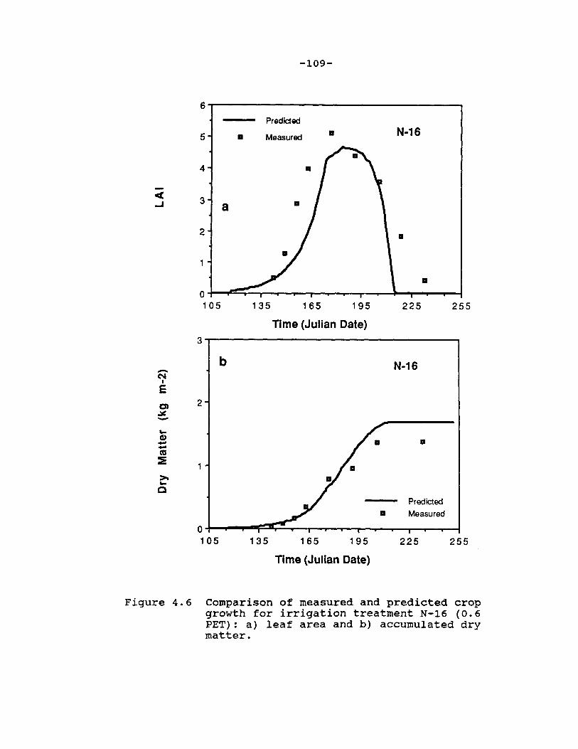
-109-

6

Predicted

5 • Measured • N-16

4

ct 3 ..J

2 • 1

• 0 105 135 165 195 225 255

Time (Julian Date)

3

b N-16 -N I

E C) 2

.::,f. -._ Cl) a --(1J

::E 1 >-._ C

Predicted

Measured

0 105 135 165 195 225 255

Time (Julian Date)

Figure 4.6 Comparison of measured and predicted crop growth for irrigation treatment N-16 (0.6 PET): a) leaf area and b) accumulated dry matter.

-110-

6

a S-16

5

Predicted

4 Ill Measured

c( 3 ..J

2 El

1 Iii

0 105 135 165 195 225 255

Time (Julian Date)

3

b S-16 -N

I

E C, 2

.:ac: -.. Predicted Q) - • Measured -as

:E 1 >, .. C

•

0 105 135 165 195 225 255

Time (Julian Date)

Figure 4.7 Comparison of measured and predicted crop growth for irrigation treatment S-16 (0.3 PET): a) leaf area and b) accumulated dry matter.

-111-

The equation modeling radiation partitioning between crop

and soil surface will effect potential transpiration and

therefore initial rate of use of soil water. More

radiation partitioned to the crop results in stress

occurring sooner. The choice of the value for critical

leaf water potential will effect the response of the

canopy resistance to leaf water potential. A less

negative value would result in earlier closure of stomates

and a concomitant reduction in photosynthetic rate,

leading in turn to lower dry matter accumulation and

reduced leaf area. Further, assumptions about root

distribution and density might not be valid for the

deficit irrigation treatments. Generally though, root

growth is assumed to be enhanced under water stress

conditions relative to shoot growth. If one assumes, that

the model is an accurate representation of the effects of

water stress on growth, the deviations observed in the

water deficit treatments could be attributed to factors

other than water, for example phosphate deficiency. While

the plant might be able to fulfill transpirational demand

by tapping water at lower depth, phosphate concentrated

mostly in the upper 15 to 20 cm of the soil profile might

be unavailable due to the extremely low water contents

there. This could also partially explain the slight

overprediction of dry matter accumulation in treatment 0.6

PET. In the field, the effect of water stress and

nutrient stress cannot be easily separated. A better

-112-

knowledge and understanding of root growing patterns and

distributions and at the same time an improved ability to

model growing root systems will enhance our understanding

of the interactions of water and nutrient stresses on

plant growth.

A comparison of final measured and predicted above

ground dry matter for seven irrigation treatments is shown

in Fig. 4.8. The slope of the linear regression of

measured on predicted total above-ground dry matter

indicates that, on the average, measured total dry matter

is being overpredicted by eleven percent. Measured field

top dry matter as a function of applied irrigation water

for amounts less than potential evapotranspiration are

shown in Fig. 4.9 b. When predicted values were plotted

for this same range of irrigation water treatments (Fig

4.9 a) it was found that the best fit regression had a

similar intercept and slope. However, the predicted

increase in dry matter with irrigation is slightly higher

than the measured one.

4.4.3 Simulation of the Dynamics of Water Stress

Leaf water potentials are one indication of plant

water stress. Simulated mid-day leaf water potentials at

14:00 hours for the four irrigation treatments are shown

in Fig. 4.10 a. As expected, the simulated leaf water

potentials of the well watered (1.0 PET) and the excess

watered (1.6 PET) treatments never attain water potentials

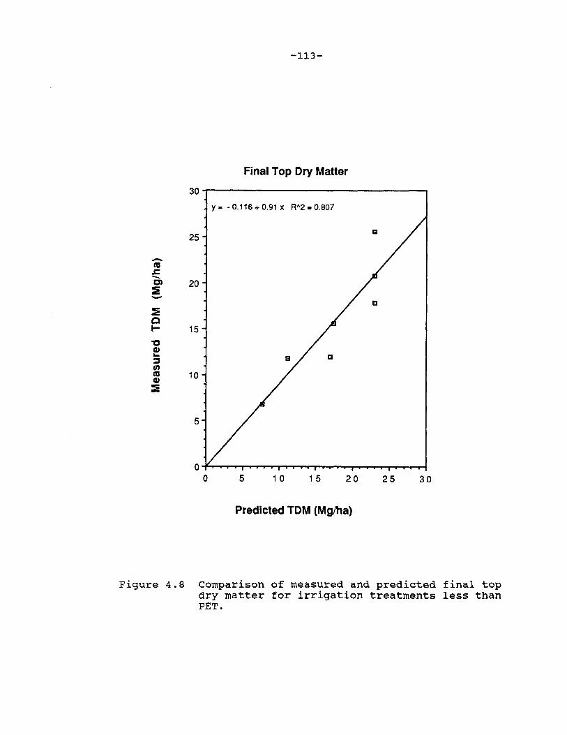
-113-

Final Top Dry Matter

30

Y• -0.116+0.91 x R"2•0.807

25

-ca .s::. --C) 20 :E - Ill

:E C t- 15 "C G) ... Ill ::, ,n ca 10 G)

:E

5

0 ..,.., ........ .,...,..-r-, ........ ,....,.."T""T .............. T""'l""T"""l ........ ,....,.. ................ T""T"' ........ --4

0 5 1 0 1 5 20 25 30

Predicted TDM (Mg/ha)

Figure 4.8 Comparison of measured and predicted final top dry matter for irrigation treatments less than PET.

-ta .t: -C,

:i -:i C t-i:, Cl) -u ·-,, Cl) a.. Q.

ci .t: -C,

:i -:i C

a 25

20

15

10

5

-114-

m

li1

TOM• - 1.0207 + 4.58788-2 IRA R"2'"' 0.885

o--------------------100 200 300 400 500 600


b Ill

25

20

t- 15 ,, Cl) a.. :, tn ta Cl)

:i

10 111

5

m

TOM • - 0.80985 + 3.93938-2 IRA R"2 .. 0.891

0-1---....---,---....--..---..---T"""""-.---...--.----1 100 200 300 400 500 600


Figure 4.9 Final top dry matter as a function of the amount of irrigation water received. a) simulated and b) measured.

-ca c.. .lll: -ca --C Q) -0 c.. ... CD -ca

== -0 0 cc

-ca c.. .lll: -·--C CD -0 c.. ... Cl) -ca

== -ca CD ...I

-115-

-100

-300 a

-500

-700

-900

-1100 -·-·--·- N-01

-1300 --·- N-11

-1500 ·····-··· N-16

S-16

\ '!, ~~ \'\ . .

' ~ ... , .... .. .. . ~, :t : .... ..... ti I U fl In f I II \ 'I I ... ...

\! •

t \ . . .. ~ ( -..:~

-1700 ........... ---....... ,_..------------....... --------------------i 11 0 130 150 170 190 210 230 250

Time (Julian Date)

-100

-300

-500

-700 ' ~ -900

-1100 -·-·-·-·- N-01

-1300 ......... _....... N-11

-1500 ·····-··· N-16

S-16 -1700 -4-....... - .............................. ,...,.. ................................. ._ ....... ________ .....

11 0 130 150 170 190 210 230 250

Time (Julian Date)

Figure 4.10 Simulated plant water potential at 14:00 hrs. a) root and b) leaf.

-116-

indicative of water stress. This is not the case for the

two water stress treatments 0.6 PET and 0.3 PET. In

treatment 0.3 PET, predicted leaf water potential drops

soon after the initiation of irrigation water treatments,

on day 132. After day 155 potentials become increasingly

negative. Treatment 0.6 PET was able to maintain higher

leaf water potentials for a longer time, but potentials

start to drop after day 180. This corresponds to the time

when observed leaf area indices start to deviate from the

well watered treatments (see Fig. 4.1 a). While

treatments 0.6 PET only deviates after day 180, the leaf

area development in 0.3 PET was delayed from the onset.

Corresponding root water potentials, which are always

slightly more positive, are shown in Fig. 4.10 a for the

same treatments. A lower limit of -1500 kPa was used and

the root water potential was not allowed to drop below

this value.

As leaf water potential become more negative, the

canopy resistance to vapor transport is affected, and

actual transpiration will be reduced from potential

transpiration (Fig. 4.11 a). The same relative reduction

as calculated for transpiration is applied to

photosynthetic rate, assuming that carbon dioxide

diffusion through the stomates is limiting photosynthetic

rate. Fig 4.11 b depicts daily totals of simulated

photosynthetic rates for the well-watered and the two

deficit treatments. The reduction in photosynthetic rate

C 0 -a, ... a. tn C a, ... I-

-C G> -0 c..

--

-,.. I

>-"' 'C

N I

E N 0 0

C') -tn ·u; G>

.J::. -C >tn 0 -0

.J::. c..

1.00

0.80

0.60

0.40

0.20

a

1.0 * PET

0.6 * PET

0.3 * PET

-117-

0.00 +-.--r __ ,_,.. __ .,....,,........,.........,.. __ ,....,. __ ,....,. __ .,....,,.......-,..-....,.. __ ...-t

110 130 150 170 190 210 230 250

Time (Julian Date)

b

~ 1.0* PET

• 0.6 * PET

100 0.3 • PET

50

0 ..J,...-=~---r-T-".......-..--..--...--.. .............. _.....1 110 130 150 170 190 210 230 250

Time (Julian Date)

Figure 4.11 Simulated water stress on a daily basis over the growing season for three irrigation treatments N-11 (1.0 PET), N-16 (0.6 PET) and S-16 (0.3 PET). a) ratio of actual to potential transpiration and b) photosynthesis.

-118-

parallels the time course of transpirational deficit (Fig.

4.11 a), although it is effected as well by the predicted

leaf area of the crop. The reduced rate of photosynthesis

will in turn translate into reduced dry matter and a

reduction in rate of leaf area expansion.

Simulated plant water potentials, actual and potential

transpiration rates, and rates of photosynthesis are shown

in Fig. 4.12 on an hourly scale for treatment 1.0 PET (1.0

PET). During the six days depicted, an irrigation event

occurred on day 203 after dusk. Leaf water potentials in

the well watered treatment drop to about - 700 kPa during

mid-day, and recover to values above - 100 kPa at night.

Actual transpiration proceeds at potential rates during

all days between the two irrigations, indicating the lack

of water stress. Simulated photosynthetic rates (Fig.

4.12 c) reach peak values of 16 g m· 2 hour· 1 around mid

day, which compares favorably with reported peak rates of

carbon dioxide fixation of 17.4 g m· 2 hour· 1 (37 mg dm·2

leaf area hour· 1 , at LAI of 4.7) reported for corn by

Stoskopf (1985), and are about 80 percent of the maximum

peak photosynthetic rate measured in corn in the Cerrado

of 22.6 g m· 2 hour· 1 (48 mg CO2 dm·2 leaf area hour·1, at

LAI of 4.7) (Luiz Carvalho, pers. communication).

In treatment 0.6 PET predicted leaf water potentials

drop rapidly between irrigations and reach values less

than -1200 kPa, below which canopy resistance increases

rapidly and leads to a reduction in potential

-119-

Figure 4.12 Simulated water stress on an hourly basis between irrigation events for treatment N-11 (1.0 PET): a) plant water potential, b) actual and potential transpiration, and c) nonwaterstressed and stressed photosynthesis.

-• A. ,¥

j -C II -0

A.

... II -ca ;:

-.,.. • • N • E Cl) ,¥ -C 0 -• .. ci. • C ca .. I-

-.,.. • ... :, 0

&.

N e N 0 C)

Q -• "ii II &. -C >,

• 0 -0 &. A.

-120-

-100

-300

-500

-700

-900 a -1100

-1300 ----- Root

-1500 - Leaf

-1700----------------------.---1 199

0.0002

0.0001

0.0000 199

b

I

~ l

' I

I I

200 201 202

Time (Julian Date)

-- Potential - Actual

~ Z' ~ I • I

I

I I

• • I I

• I ' I

200 201 202

Time (Julian Date)

203 204 205

:·

' I I

I

• • ' I

' • I

I • I I

203 204 205

20-----------------------, C -- Non-stressed

-- Actual

15

10

5

0 ~-__. .... - ........ ----...... -..-........ ----......... --.-..... "" 199 200 201 202 203 204 205

Time (Julian Date)

-121-

transpiration and concomitant reductions in photosyn

thetic rate (Fig. 4.13). Both recover rapidly the morning

after the irrigation on day 203, although water potentials

in 0.6 PET do not recover fully to non-stressed levels.

Predictions of root water uptake have been shown to be

more sensitive to rooting depth than to root density (Da

Silva and de Jong, 1986). Limiting the maximum rooting

depth obtainable had no effect on predictions of actual

transpiration in treatment 1.0 PET. In the water-stress

treatments predicted actual transpiration and dry matter

accumulation were reduced when rooting depth was not

allowed to exceed a maximum value in the simulation (Table

4.2).

Stoeckle and Campbell (1985) presented a correlation

between water stress accumulated during pollination (Sip)

and the harvest index (HI), which did not apply well to

the experimental results and simulations presented here.

Predicted harvest index using their regression equation on

accumulated stress index during pollination and measured

harvest index are compared in Table 4.3. Measured harvest

index in this experiment was poorly related to predicted

accumulated stress during pollination (Fig. 4.14 a), but

more closely related to total accumulated stress during

the whole growing season (Fig. 4.14b).

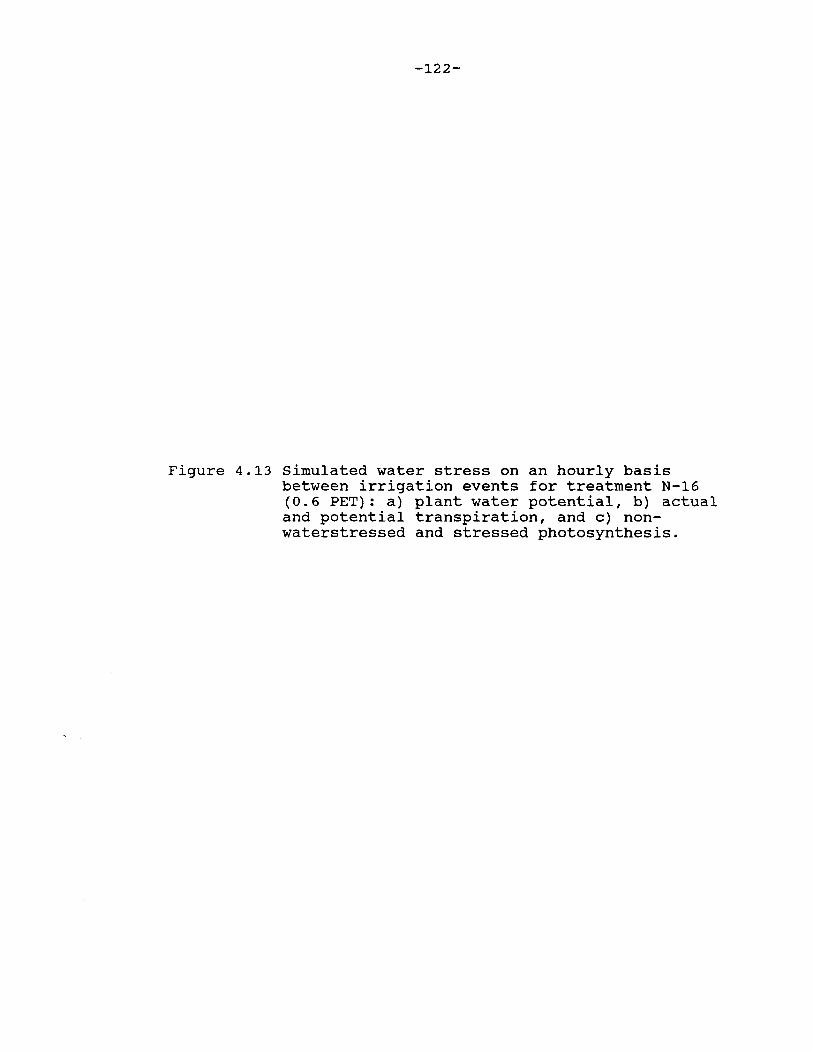
-122-

Figure 4.13 Simulated water stress on an hourly basis between irrigation events for treatment N-16 (0.6 PET): a) plant water potential, b) actual and potential transpiration, and c) nonwaterstressed and stressed photosynthesis.

• a. ~ -.!! -C • -0 a. .. • -• :it

..... .... . • N • E

Q ~ -C .2 -• .. Q. • C ca .. ....

..... .... • .. :I 0 .c. N

E N 0 (J

-123-

-100

-300

-500

-700

-900

-1100

-1300

-1500

-1700 199 200 201 202 203

Time (Jullan Date)

0.0002 ---- Potential - Actual

I

~ I

I I

0.0001 ' ' I

' I I

I I

I I • 0.0000

199 200

:· r • I I

n I r '

• ' I

I

201 202

Time (Jullan Date)

I

203

204 205

' I

I • I

I I

A I

I I I '

'

I , I

204 205

20------------------------. C - Non-stressed

- Actual

15

a, 10 -.!! • • .c. -C >,

• 0 -0 .c. a.

5

0 ..... ..._ ............. __ ,..._.,.....,...,_....,.. ... -.__,-.... .,._ ........ -I

199 200 201 202 203 204 205

Time (Jullan Date)

-124-

0.30

>< a HI • 0.246- 0.017 Sl(p) R112 • 0.679

Q) ,, C 0.25 -U) Q)

> ... as 0.20 :c ,, Q) ... :, ,n 0.15 as Q)

~

0.10 0 1 2 3 4 5 6

Stress Index (p)

0.30 b

>< HI• 0.28 - 0.015 SI Q) ,, R112"' 0.954

C 0.25 m -,n Cl) > ... as 0.20 :c ,, Cl) ... ::, ,n 0.15 as Cl)

·~

0.10 -+--...------...-~----...-----.------""I 0 2 4 6 8 1 0 1 2

Accumulated Stress Index

Figure 4.14 Measured harvest index as a function of accumulated water stress during a) pollination and b) the whole growing season.

-125-

TABLE 4.2

Simulated effects of limiting potential maximum rooting depth {0.38 m, 0.53 m, 0.75 m, and 1.05 m) on actual {mm/day) / potential transpiration {mm/day) {TR), deep drainage {mm) (DR) and final above-ground dry matter {kg/m2) {Y) under different irrigation water treatments.

Irrigation treatment

1. 0 PET 0.6 PET 0. 3 PET

TR DR y TR DR y TR DR

0.38 m :

y

363/364 70 2.30 164/201 13 1.32 75/145 11 0.56

O. 53 m :

364/364 69 2.30 177/211 11 1.45 87/154 9 0.65

0.75 m :

364/364 68 2.30 193/223 9 1.59 102/161 7 0.77

1. 05 m . . 364/364 67 2.30 208/232 5 1. 69 102/161 7 0.77

-126-

TABLE 4.3

Harvest index estimated from experimental data (Him), and predicted (HIP) from accumulated stress during pollination ( SIP ) •

Irrigation (mm)

509

430

327

316

188

SI 1 p

0.01

0.29

0.36

5.25

5.96

SI 2 t

0.04

3.68

4.70

6.88

10.86

0.479

0.463

0.458

0.165

0.122

1 - SIP predicted from regression from stockle and Campbell (1985)

0.277

0.246

0.198

0.193

0.118

2 - Sit is the total accumulated stress index for the whole season

4.4 SUMMARY AND CONCLUSIONS

The assumptions relating to the effect of water stress

on crop growth inherent in the crop simulation model

(Stockle and Campbell, 1985) used here, appear to be valid

when applied to Cerrado conditions. Temperature and light

effects on photosynthesis are considered in the

calculation of a non-stressed photosynthetic rate, which

is dependent on the amount of photosynthetically active

radiation intercepted by the canopy. Thus, model

predictions are sensitive to the predicted partitioning of

potential evapotranspiration. Photosynthetic rate in the

model is reduced when leaf water potentials drop below a

critical leaf water potential for stomatal closure. The

-127-

reduced photosynthetic rates translates directly into

reduced dry matter accumulation and a reduced leaf area.

Water stress is accumulated as a water stress index and

effects the reduction of leaf area index after the end of

the vegetative phase.

Predicted leaf area indices and dry matter

accumulation over time compared well with measured data.

Dry matter and leaf area were overpredicted in the most

extreme water stress treatment, possibly due to soil

fertility/water interactions not represented in the model.

Important parameters effecting predictions are leaf area

ratios, which vary with variety and were shown to decline

over time for the variety used here, while an average leaf

area ratio was used in the simulations. Model predictions

are sensitive to the time, when phenological stages of

pollination and maturity are reached. Simulated final dry

matter is very sensitive to the thermal time chosen for

maturity, since further dry matter accumulation is

discontinued after the crop reaches maturity.

Harvest index was related more to water stress

accumulated throughout the growing season, than to water

stress accumulated during pollination, as was suggested by

Stockle and Campbell (1985).

Hourly predicted leaf water potential changes and

corresponding changes in transpiration and photosynthetic

rate represented the dynamics of water stress

realistically and were consistent with expectations.

-128-

REFERENCES

Acevedo, E. 1975. The growth of maize (Zea mays L.) under field conditions as affected by its water relations. Ph.D. thesis, Univ. of California, Davis. 253 p.

Bandy, D. 1976. Soil-plant=water relationships as influenced by various soil and plant management practices on Campo Cerrado soil in the Central Plateau of Brazil. Ph.D. thesis, Cornell University, Ithaca. 236 p.

Buttler, I. W. and S. J. Riha. 1987. General purpose simulation model of water flow in the soil-plantatmosphere continuum. Appl. Agr. Res. 2:230-234.

Buttler, I. W. ands. J. Riha. purpose simulation model of atmosphere. User's manual. University, Ithaca, NY.

1988. GAPS - A general the soil-plant-Version 1.1. Cornell

Campbell, G. s. 1985. Soil physics with BASIC: Transport models for soil-plant systems. NY Elsevier.

Coelho, D. T. and R. F. Dale. 1980. An energy-crop growth variable and temperature function for predicting corn growth and development: planting to silking. Agron. J. 72:503-510.

Dale, R. F., Coelho, D. T., and K. P. Gallo. 1980. Prediction of daily green leaf area index for corn. Agron. J. 72:999-1005.

Fisher, M. J., Charles-Edwards, D. A., and M. M. Ludlow. 1981. An analysis of the effects of repeated short term soil water deficits on stomatal conductance to carbon dioxide and leaf photosynthesis by the legume Macroptilium atropurpureum cv. Siratro. Aust. J. Plant Physiol. 8:347-357.

Foth, H. D. 1962. Root and tap growth of corn. Agron J. 54:49-52.

Gonzales-Erice, E., Kamprath, E. J., Naderman, G. c., and W. V. Soares. 1979. Effect of depth of lime incorporation on the growth of corn on an Oxisol of central Brazil. Soil Sci. Soc. Am. J. 43:1155-1158.

Goodwin, J. B., Garacorry, F. L., Espinoza, w., Sans, L. M., and L. J. Youngdahl. 1982. Modelling soil-waterplant-relationships in the Cerrado soils of Brazil: The case of maize. Agric. Systems 8:115-127.

-129-

Hanks, R. J., Keller, J., Rasmussen, V. P., and G.D. Wilson. 1976. Line source sprinkler for continuous variable irrigation-crop production studies. Soil Sci. Soc. Am. J. 40:426-429.

Hesketh, J. and D. Baker. 1967. Light and carbon assimilation by plant communities. Crop Sci. 7:285-293.

Macedo, J. and R. B. Bryant. 1987. Morphology, mineralogy, and genesis of a hydrosequence of Oxisols in Brazil. Soil Sci. Soc. Am. J. 51:690-698.

Monteith, J. L. 1981. Climatic variation and the growth of crops. Q.J.R. Meteorol. Soc. 107:749-774.

Norman, J.M. 1982. Simulation of microclimates. "Biometeorology in integrated pest management". Academic Press, New York.

Norman, J.M., and G. S. Campbell. 1983. Application of a plant-environmental model to problems in irrigation. Adv. Irrig. 2:155-188.

Priestley, c. H.B. and B. J. Taylor. 1972. On the assessment of surface heat flux evaporation using large-scale parameters. Mon. Weather Rev. 100:81-92.

Riha, s. J. and G. s. Campbell. 1985. fluxes in Douglas-fir plantations. 15:701-707.

Estimating water Can. J. For. Res.

Ritchey, K. D. 1982. Calcium deficiency in clayey Bhorizons of savanna Oxisols. Soil Sci. 133:378-382.

Stockle, c., and G. s. Campbell. 1985. A simulation model for predicting effect of water stress on yield: an example using corn. Adv. in Irrigation 3:283-323.

Stoskopf, N. c. 1985. Cereal Grain Crops. Reston Publishing, Reston. Virginia. 516 p.

Turner, N. C. 1974. Stomatal behavior and water status of maize, sorghum and tobacco under field conditions at low water potential. Plant Physiol. 53:360-365.

Wolf, J.M. 1975. Water constraints to corn production in Central Brazil. Unpublished Ph.D. Thesis, Cornell University.

Chapter V

SUMMARY AND CONCLUSIONS

The objective of the research program of which this

project is a part is to determine crop water requirements

for the Cerrado region of Brazil. Knowledge of the

influence of evapotranspiration, soil hydraulic properties

and water management on crop growth is important for both

the agronomic and economic evaluation of irrigation

development and the extension of rainfed agriculture. In

the case of irrigation a knowledge of crop water

requirements in relation to yield will allow for better

irrigation planning and design, as well as more realistic

comparison of the relative benefit of using water for

irrigation rather than for other purposes. In the case of

rainfed agriculture, such knowledge will allow for more

realistic evaluation of the feasibility of extending

agriculture into areas where dry spells during the wet

season are likely to reduce yield potential, as well as

establish a basis for improving crop tolerance to short

droughts.

The relationship between evapotranspiration, soil

water properties and crop growth is complex. For this

reason, dynamic plant-environmental simulation models were

developed and used to predict water budgets and crop

growth under a range of irrigation water treatments.

Specifically, a microcomputer-based program (GAPS} was

-130-

-131-

designed to allow construction of several simulation

models from various mathematical representations of

processes in the soil-plant-atmosphere system. These

representations, for the most part, had been previously

published but not extensively tested, especially by

researchers other than the group responsible for their

development. The use, testing, and refinement of

previously published models was considered important in

this research program both to test their applicability to

regions of the world for which they were not originally

developed (and thus determine the generality of the

underlying assumptions) and to build on existing paradigms

that have shown to work reasonably well.

The structure of GAPS allows for direct comparison of

various representations of evapotranspiration, soil water

flow, crop water uptake and crop growth. Two different

representations of soil water flow and plant water uptake

were considered in this study: a) a capacity-type water

flow model (Tipping Bucket) combined with a plant water

uptake model based on the concept of plant-available

water, and b) a numerical solution to the Richards

equation combined with a potential driven water uptake

model. Both used the Priestley-Taylor method to estimate

potential evapotranspiration. To test the applicability

of these models to Cerrado conditions in the Cerrado of

Brazil, a line source sprinkler experiment which provided

a range of irrigation water application to corn from 0.3

-132-

to 1.6 potential evapotranspiration was established during

the dry season of 1987.

Both the Richards equation and the Tipping Bucket

routine simulated soil water contents well under a wide

range of irrigation water treatments. The advantages of

the Richards equation are that it better predicts the

water content distribution in the soil profile, gives more

continuous predictions of water fluxes, and provides

estimates of water potentials as a function of time and

space that can be linked to potential-driven root water

uptake and crop growth procedures. However, the water

content-potential relationship for this Oxisol was not

well described by the Campbell moisture release equation,

which assumes that the log-transformed moisture release

data is linear. Furthermore, field satiated water

contents, which are around 70% of total porosity, had to

be known in order to predict water contents correctly.

Soil compaction, as indicated by increased bulk densities,

did not change satiated water contents in proportion to

the decrease in total pore volume, presumably because the

portion of porosity lost due to compaction was not water

filled at satiated water contents under non-compacted

conditions. The Tipping Bucket routine was very sensitive

to the value chosen for field capacity. The capacity-type

water uptake procedure linked to the Tipping Bucket

routine compared well with the potential-driven root water

uptake procedure used together with the Richards equation,

-133-

especially under water-limiting conditions. The limited

available data on rooting depth and relative root

distributions together with the assumptions used in the

root growth simulations seemed to provide satisfactory

results, judged by the comparison of observed and

predicted soil water extraction patterns. Advection was

identified as a plausible factor in underpredicting

evapotranspiration during the later part of the dry

season.

The corn growth simulation model was developed and

tested previous to this study for another variety of corn

grown in California. Although this model was considered

crop-specific by its developers, only a few procedures are

based on empirical relationships derived from corn. These

include the photosynthetic rate as a function of PAR, leaf

area development and leaf area ratio. The model predicted

the effects of water stress on leaf area development very

well and also predicted the relative effect of water

stress on above-ground dry matter accumulation. Final

predicted above-ground dry matter production was

approximately 11% higher than measured. Measured values

ranged from 6 Mg/ha for an irrigation treatment equivalent

to 0.3 PET to 25 Mg/ha at 1.6 PET.

The assumptions relating the effect of water stress to

corn dry matter accumulation and leaf area development

used in the growth component models appear to apply to

Cerrado conditions. Predicted time courses of dry matter

-134-

accumulation and leaf area development compared well with

measured data under a range of irrigation water

treatments. The model predictions were sensitive to the

partitioning of potential evapotranspiration.

Partitioning more PET to transpirational demand in the

early season led to faster development of water stress

effects under the deficit irrigation treatments. The leaf

area ratio used to convert dry matter to leaf area

strongly effects early leaf area development and

predictions of dry matter production. The critical leaf

water potential used to increase canopy resistance as a

function of leaf water potential will determine how soon

potential transpiration (and thus photosynthesis) respond

to water stress. The date of maturity used to end further

dry matter production is critical in its effect of final

yields. Reduced growth under the extreme water stress

treatment appeared to be due to additional factors,

possibly nutrient deficiency caused by the extremely dry

topsoil.

We conclude that the linked water and crop growth

model can generally predict water movement in Cerrado

soils and can predict the water stress on corn yield. The

model could be applied for irrigation planning purposes

and prediction of the effects of dry spells on crop growth

in the rainy season.

This study has also demonstrated that developing

software that allows for multiple representations of

-135-

plant-environmental processes is a promising approach that

should result in more extensive and continued improvement

of plant-environmental simulation models.

-136-

APPENDIX A

GAPS User's Manual

-137-

G A P S

A ~eneril furpose ~imulation Model

of the

Soil-Plant-Atmosphere System

Version 1.1

User's Manual

(DRAFT)

by

Imo W. Buttler and Susan J. Riha

Cornell University

-138-

Acknowledgements

We would like to acknowledge several people who contributed, either

directly or indirectly, to this program.

Prof. Gaylon Campbell greatly influenced both authors' approach to

simulation modeling when they worked with him at Washington State

University and through his recently published "Soil Physics with BASIC"

(Elsevier).

Oner Bicakci played an instrumental role in designing the user

interface, particularily the screen menus. Jennifer Sanchez assisted in

the production of the dependency diagrams and proofread portions of the

documentation. James Altucher helped trouble-shooting later versions of

the program and developed much of the current version of the Plotter.

This program was developed as part of the doctoral research

conducted by the senior author and supported in part by subgrant SM

CRSP-012 of the TropSoils program funded by USAID.

-139-

Table of Contents

I . Introduction to GAPS 1.1 GAPS Menus

2.

1.2 Getting Started

Editor 2.1 Input

2 .1.1 2 .1.2 2.1.3 2.1.4 2.1.5

Data Files Climate Data File Soil Data File Plant Data File Location Data File Output Format File

3. Simulator 3.1 Introduction 3.2 Documentation of Modules

3.2.1 Solar_Angles 3.2.2 Atmos Trans 3.2.3 Air_Temperature

3.2.4 Priestley_Taylor_ETP 3.2.5 Penman ETP 3.2.6 Pan ETP 3.2.7 L inacre ETP

3.2.8 Max_Photosynthesis 3.2.9 Critical Leaf Water 3.2.10 Growth Stages

Potential

3.2.11 Dry_Matter_Accumulation

3.2.12 Richards_Equation 3.2 .13 Tipping_Bucket_Flow 3.2.14 Water_Budget

3 .2 .15 Water_Uptake 3.2.16 Simple_Water_Uptake

3.2.17 Soil Temperature 3.2.18 Const Soil Temp - -

3.3 Linking modules 3.4 Run Time Plotting 3.5 Saving Output to Files

-140-

1. Introduction to GAPS

GAPS is a general purpose simulation model of the soil-plant

atmosphere system. GAPS is programmed in TurboPascal 4.0 and can be

implemented on the IBM PC/AT or fully IBM PC compatible computers. The

program consists of three main parts: the Editor, the Simulator, and

the Plotter. The Editor allows the user to create or edit all files

that are necessary input to the simulator. The Simulator links and

implements the simulation procedures selected by the user. The Plotter

outputs results of a simulation run or input data files to a printer.

This manual is organized in three major sections. Chapter 2

describes the structure and function of the Editor and the structure of

input data files. Chapter 3 contains the documentation of the currently

existing procedures in the Simulator. Each procedure is documented in

detail in a separate chapter. Some information on how to make changes

to an existing procedure and on how to add additional procedures to the

Simulator is contained in Appendix B. Changing existing procedures or

adding new ones requires some programming experience. Chapter 4

introduces the user to the functions of the Plotter. The Plotter is the

part of the program responsible for accessing simulation model output or

input. Note that instantaneous output can be obtained during the

simulation run using the run time plotting option (see Chapter 3.4).

1.1 GAPS Menus

The intention of GAPS is to provide a user friendly environment in

which to use simulation models. All the interaction with the user is

through menus. The menus used in GAPS all follow the same general

-141-

layout. The screen is partitioned into several windows in which

different information is displayed. The main window contains the

different options available to the user at a particular level in the

program. The function keys on the left side of the screen are used to

facilitate user response. The function keys correspond to the options

displayed in the main window and their definition changes between

different windows. If no function keys are available the user can

respond with the first letter of the respective choice. In the lower

right hand window input data file currently residing in memory are

displayed after they have been loaded in by the user before running a

simulation.

1.2 Getting Started

To run GAPS insert the GAPS runtime diskette into one of your disk

drives and type 'RUNGAPS'. This will execute a batch file that will

automatically change the default directory to the already created

subdirectory \GAPS\DATA, where test versions of input data files reside

and where you will store your own data files. It will then invoke GAPS.

Before running a simulation program the input data files have to be

loaded into memory. Once all the necessary files are loaded and their

names are being displayed in the lower right hand corner of the screen,

you are ready to construct a simulation model from the component parts

currently existing in the simulator. Choose the option 'Procedures'

from the Simulator menu. A new menu will appear giving you the choice

between different component parts of the system such as 'Water Flow',

'Water Uptake', 'Potential Evapotranspiration', and 'Soil Temperature'.

-142-

Upon selecting one or more of these options, you will have to select

between different representations of the respective process. You can

also specify the first and last day of the simulation run and choose the

time step to be used (option 'Time'), and select up to four variables to

be plotted instantaneously on the screen during the simulation run

(option 'View'). If you want to save output to disk, option 'Out' needs

to be selected and filenames identified. Hourly and/or daily data can

be saved and the days and hours when to save data can be determined (see

Chp. 3.5) When you made all your selections you may choose 'Run' to

actually run the simulation. After the simulation stops you can hit any

key to return to the simulator menu. You can change any of your options

in terms of input data files or the constellation of the simulation

model and execute another run. If you want to have a hard copy of the

plots generated during the simulation run you can dump them to the

printer (shift-PrTSc).

After a run you can enter the Plotter via the GAPS main menu and

obtain further output from the simulation model. You can obtain tabular

output of the main variables that have been saved to a file during the

simulation run.

For detailed information about the procedures currently contained

in the Simulator please refer to Chapter 3, where each procedure is

documented in detail in a separate chapter.

-143-

2. The Editor

2.1 Editing Data Files

All the interaction between GAPS and the user is through menus.

The Editor can be entered from the GAPS main menu by selecting the

appropriate function key (Fl) or, if function keys are not available, by

hitting the corresponding first letter of the respective choice, in this

case by hitting an 'E' for 'Editor'. Upon choosing the Editor option,

the Editor menu will appear. The user is given the choice which

category of input data files to edit (Climate, Soil, Plant, or Location

Files). Upon choosing one of the categories the respective menu will

appear. The option 'Outp' lets the user specify on which days and at

which hours to save simulation output to disk. Since the internal data

structure of the input files is different in each case, the options

available for editing the data files are too.

The Editor searches the default directory for existing files of the

desired type (reckognized by a particular file extension) and displays

the file names in the window at the center of the screen. The user can

use the arrow keys to scroll up and down the list and select any of the

files for further editing (option 'Load'). To construct a new file, a

file name (without specifying a file extension) has to be given, and the

'Make' option selected. A blank spreadsheet in the format of the data

file will appear on the screen and the user can input data.

Selecting the 'Quit' option in any of the menus will bring the user

back to the next higher level menu and, if hit consecutively back to the

GAPS main menu and eventually back to DOS.

-144-

Existing input data files can be accessed from the GAPS Plotter and

printed (see Chp.4.2). A user does not have to provide all parameters

included in an input file. Only the parameters used in a specific

application have to be present. For example, to use the

Richards Equation procedure to simulate water flow, values for wilting

point or field capacity are not needed. The corresponding spaces in the

input file could be left blank.

2.1.1 Editing a Climate Data File

A Climate Data File can contain a maximum of one years' of data

{365 days). Row #1 in the file corresponds to January 1, row #365 to

December 31. If a climate data set starts for example on June 01, the

first row to input data would be #152. The user can jump to any row

(date) in the file by using the 'Jump' option. 'Insert' can be used to

input data for the first time or to insert additional days of data in an

existing file. 'Modify' allows changing data entries. Simply hit

return for the parameters you do not want to change. 'Save' will save

the file to the disk. Note that you can change the file name and thus

save an edited version of the file under a different name. 'Load' will

load an existing file into the Editor.

At this time the Editor only accepts daily climate data.

Parameters included in the current version of the climate input file are

listed below. The variable name, units, and procedures in which they

are used are also given. In the computer code, all climate data

variable names are preceded by the prefix 'clim.', e.g. clim.MaxTemp.

-145-

1. Maximum air temperature, MaxTemp, degrees C ( ... _Temperature-

... _ETP)

2. Minimum air temperature, MinTemp, degrees C ( " )

3. Solar radiation, SolRad, MJ m- 2 d- 1 (Atmos Trans, ... _ETP)

4. Precipitation, Precip, mm d- 1 ( ... _Flow)

5. Relative humidity, RelHumid ( ... ETP, Richards_Flow)

6. Wind speed, WindSpeed, m s-1

7. Pan evaporation, PanEV, mm d- 1 (Pan ETP)

2.1.2 Editing a Soil Data File

A soil data file contains information on soil parameters as a

function of depth. Any number of soil layers up to 20 can be specified

and different properties can be assigned to each soil layer. The depth

of each layer can be chosen by the user when setting up the soil data

file. When using the numerical solution to the water flow equations the

user should be aware of the effect of node spacing and time step size on

the results of the numerical solution. Close node spacings at the soil

surface are recommended. Parameters included in the current version of

the soil input file are listed below. In the code, all soil input

parameters carry the prefix 'soil.', as for example in soil.NodeDepth.

1. Node depth, NodeDepth, m ( ... _Flow, ... _Temperature, ... _Uptake)

2. Bulk density, BulkDens, Mg m- 3 ( ••• _Flow, Soil_Temperature,

... Uptake)

3. Particle density, PartDens, MG m- 3 ( ... Flow)

4. Saturated hydraulic conductivity, HydCond, kg s m- 3

(Richards_Flow)

-146-

5. Air Entry potential, AirEntryPot, J kg- 1 (Richards_Flow}

6. Soil B-value, BValue, (Richards Flow)

7. Initial node water content, InitWater, m3 m- 3 ( ••• _Flow}

8. Field capacity water content, DUL, m3 m- 3 (Tipping Flow}

9. Wilting point water content, LL, m3 m- 3 (Tipping_Flow,

Water_Budget)

10. Initial soil temperature, InitSoilTemp, degree C (Soil_Temp)

Empirical equations to estimate some of these parameters can be

found in Appendix C.

2.1.3 Editing a Plant Data File

At this point GAPS does not contain any crop growth components. A

static crop can be defined in terms of leaf area index and several root

parameters. The plant data file contains the following parameters. The

prefix for plant input variables is 'plant.', as for example in

plant.LAI.

1. Initial leaf area index, LAI, (Canopy)

2. Root radius, RootRad, m (Water Uptake)

3. Root density, RootDens, m m- 3 (Water Uptake)

4. First layer containing roots, FRoot (Water Uptake}

5. last layer containing roots, NRoot (Water_Uptake}

6. Root resistance, RootRes, (Water Uptake}

7. Emergence date, EmergenceDate

8. Initial canopy height, CanopyHeight, m

9. Initial dry matter, InitialDryMatter, kg m-2

10. Maximum water interception capacity, MaxCanopy, mm

-147-

11. Resistance of open stomates, RCopen, s m-1

12. Critical leaf water potential, Critical_LeafWP, J kg-1

13. S parameter, S, (Critical_LWP)

14. Aerodynamic resistance, RA, s m-1

The user can scroll through the list of variables and input values

for these parameters or change existing ones much in the same way as has

been explained above.

2.1.4 Editing a Location Data File

The Location information contains the following site specific

parameters. All location parameters carry the prefix 'loca.' in the

code, for example loca.LAT.

1. Latitude, LAT (Solar Angles)

2. Time of solar noon, TSN (Solar Angles)

3. Priestley-Taylor Alpha value, ALPHA (Priestley_Taylor_ETP)

4. Short-wave absorptivity of the surface, AS( ... ETP)

5. Long-wave emissivity of the soil or canopy surface, ES( ... ETP)

6. Resistance to heat transport, RT, s m-1 (Penman ETP)

7. Resistance to vapor transport, RV, s m-1 (Penman ETP)

8. Boundary layer conductance, Cond, W m- 2 K- 1 (Soil_Temperature)

9. Pan coefficient, Kp (Pan_ETP)

10. Crop coefficient, Kc (Pan ETP)

11. Finite difference weighing factor, F (Soil_Temp)

12. First hour of rain/ irrigation, RainFirst

13. Last hour of rain/ irrigation, RainLast

-148-

14. Elevation, elevation, m

15. Height of wind measurement, WindHeight, m

The menu is structured in a similar fashion as the plant editor menu.

2.1.5 Output Format File

If simulation output is to be saved to disk, the 'Out' option in

the simulator menu has to be activated and output file name have to be

specified (see Chpt. 3.5). The output format file can be used to

specify on which days and at which hours to save output data. If a

number greater than zero is specified for either 'Number of days' or

'Number of hours', the program will prompt you for the day or hour

numbers, respectively, when you modify the 'days' or 'hours' options.

This format file needs to be saved to be later called up from the

simulator in conjunction with output file names.

3. The Simulator

3.1 Introduction

The purpose of this part of the GAPS user's manual is to allow the

users of GAPS to understand all the equations, the solutions to the

equations, the variables and constants used in each procedure. The user

should understand these procedures for two reasons. First, the users

must select between certain procedures depending on their objective and

input data restrictions. Secondly, the user may wish to change certain

parts of the procedure or add a new procedure. Understanding the

-149-

material in this manual is the first step in enabling the user to

accomplish this.

This section documents all the procedures currently contained in

the Simulator. It will be appended as additional procedures become

available. To support the modular structure of the Simulator each

procedure is documented in a separate chapter. Each chapter contains an

explanation of the concepts and equations used in the procedure, a

dependency diagram for the procedure, where considered appropriate, the

computer code of the procedure, and a list of all variables used in the

procedure. Where appropriate, these concepts and equations are

referenced. All constants and variables used in an equation are given

the same symbol in the documentation as they have in the computer

program. All symbols are defined immediately after they are presented

in a chapter, at the end of the chapter, and again in alphabetical order

in the Dictionary (Chpt. 3.4). When a symbol is defined its dimensions

are also specified. If it is a constant, its value is also specified.

The dimensions of all variables and constants in the Simulator are in SI

(Systeme Internationale) units.

Dependency diagrams are used to illustrate the flow of information

from outside the procedure into the procedure, the main relations of

variables inside the procedure, and the output variables that leave the

procedure. The procedure presented in each chapter is represented by a

large white box in the dependency diagram. Other procedures which

produce variables that are needed as input for the main procedure are

represented as smaller shaded boxes to the left of the main procedure.

The variables produced by these other, shaded procedures are listed in

-150-

the shaded portion of the box. These variables are global variables

because they are used in more than one procedure. They are defined in

the chapter where they appear in equations and again at the end of each

chapter under the heading 'Global Variables'. Important local variables

appear in the main white box. Variables generated by the main procedure

which are subsequently used by other procedures are indicated by arrows

pointing to shaded boxes at the bottom of the diagram. These variables

are also global variables.

The dependency diagrams should not be confused with traditional

flow charts of computer programs. They merely intend to introduce users

graphically to the structure of the procedure and help them visualize

the general flow of information to, within, and from a procedure. The

dependency diagrams might be a helpful reference when making changes to

a particular procedure.

The procedure program (computer source code) is presented along

with the dependency diagram. The program begins with the procedure

title followed by a comment statement summarizing the objective of the

procedure. Then local variables and constants are defined. This is

followed by the solutions of the equations used to generate the

necessary output variables.

A list of variables and constants used in each procedure follows

the procedure program. Global variables that are output of the

procedure are starred. Finally each chapter contains a list of

references for the concepts, equations, numerical solutions and

constants used in the procedure. Specific instructions on how to add a

-151-

new procedure and how to change an existing one are contained in

Appendix D.

3.2 Documentation of modules

The first section of the GAPS Simulator uses various daily climate

data to calculate or estimate climate data needed for input to other

routines. Procedure Air_Temperature simulates hourly air temperatures

given daily maximum and minimum air temperatures Procedure Solar_Angles

uses latitude, day of the year and hour of the day to calculate the

maximum solar irradiance. The procedure Atmos_Trans uses daily measured

solar radiation to estimate an atmospheric transmission coefficient, for

use in ••• _ETP procedures that need net radiation as an input.

The second section of the GAPS Simulator currently contains four

routines to estimate evapotranspiration: Priestley_Taylor_ETP,

Penman_ETP, Pan_ETP, and Linacre ETP. The user can choose one of these

depending on the particular objective and input data available.

The procedure Max_Photosynthesis calculates photosynthetic rate on

the basis of photosynthetically active radiation intercepted by the

canopy. Photosynthesis is directly related to dry matter accumulation

in Dry_Matter_Accumulation. Growth is linked to water stress in

procedure Critical_Leaf_Water_Potential. Growth_Stages allows to define

different phenological stages using growing degree days.

Two alternate routines are available for simulating water flow

through soil. The Richards_Equation procedure uses a numerical solution

to the Richards equation to predict water flux and water potentials with

depth and time. Actual soil evaporation is also calculated. The

-152-

Tipping_Bucket_Flow procedure uses a procedure for water flow adapted

from the CERES maize model.

There are two different routines available for predicting water

uptake by plants. Water_Uptake is a potential driven resistance

approach, where water uptake is limited by a minimum root water

potential. Simple_Water_Uptake uses an adsorption approach, where water

uptake is limited by the volumetric water content at wilting point. The

former routine can only be used with the Richards_Flow procedure, since

it uses soil water potentials.

The user has the option to use the procedure Soil_Temperature which

numerically solves the heat transport equation predicting soil

temperature as a function of depth and time or to specify a constant

soil temperature profile.

List of currently available Procedures:

Solar Angles Atmos-Trans Air_Temperature

Priestley Taylor ETP Penman ETP -Pan ETP Linacre ETP

Max Photosynthesis Critical Leaf Water Potential Growth StagesDry_Matter_Accumulation

Richards Flow Tipping Bucket Flow Water_Budget -

Water Uptake Simple_Water_Uptake

Soil Temperature Const_Soil_Temp

-153-

3.2.1 Procedure Solar_Angles

This procedure calculates the solar elevation angle for any given

latitude, day of the year and hour of the day. First, the solar

declination angle (angle which the sun's rays make with the earth's

equatorial plane) is calculated knowing the day of the year. Then, the

solar elevation angle is calculated on an hourly basis from the solar

declination angle, latitude and time of day in relation to solar noon

(when the sun is directly north or south of the point of observation).

Knowing the solar elevation angle and the solar constant, i.e. the mean

annual radient flux density outside the earth's atmosphere and normal to

the solar beam (1360 W rn- 2), the theoretical irradiance above the

atmosphere can be estimated.

The irradiance above the atmosphere (SpaRad, W m- 2) at any time

during the day can be calculated according to Campbell (1977):

(1) SpaRad = SolElA * SolarConstant

where: SolarConstant is the solar constant (1360 W m-2) SolElA is the sine of the solar elevation angle (degrees) at the

time of the day

The sine of the solar elevation angle (SolElA) for any time of the

day can be calculated as (Campbell 1977, 1985):

(2) SolElA = SolDcA * sin(loca.Lat*0.01745) + cos(loca.Lat*0.01745)

* cos(0.2618*(Time-loca.Tsn)/3600)) * CSo1DcA

where: So1DcA is the sine of the solar declination angle CSo1DcA is the cosine of the solar declination angle loca.Lat is

the latitude (degrees) loca.Tsn is the time of solar noon (sec) Time is the time of the day (sec).

-154-

To determine solar noon accurately for a particular geographic location

see Gates (1980).

The sine of the solar declination angle (SolDcA) can be computed

according to Swift (1976):

(3) SolDcA = 0.39785 sin [4.869 + 0.0172 JulDay + 0.03345 sin(6.224 +

0.0172 JulDay)]

where: JulDay is the day-of-year number or Julian date, i.e. January 01 = 1,

December 31 = 365.

Solar elevation angles are calculated for every time step of the

day and, if the angles are positive, the theoretical solar radiation for

the hour is calculated. Before starting a daily loop the procedure is

executed once for the whole day to arrive at an estimate of total

theoretical solar radiation (SpaceSum). This value is needed to get an

estimate of fractional cloud cover, which is calculated in procedure

AtmosTrans.

List of References

Campbell, G.S. 1985. Soil physics with BASIC. Elsevier, Amsterdam. 150 pp.

Campbell, G.S. 1977. An introduction to environmental biophysics. Springer Verlag, New York. 159 pp.

Gates, D.M. 1980. Biophysical Ecology. Springer, New York. Appendix 4, p. 572.

Swift, L.W. 1976. Algorithm for solar radiation on mountain slopes. Water Res. Res. 12:108-112.

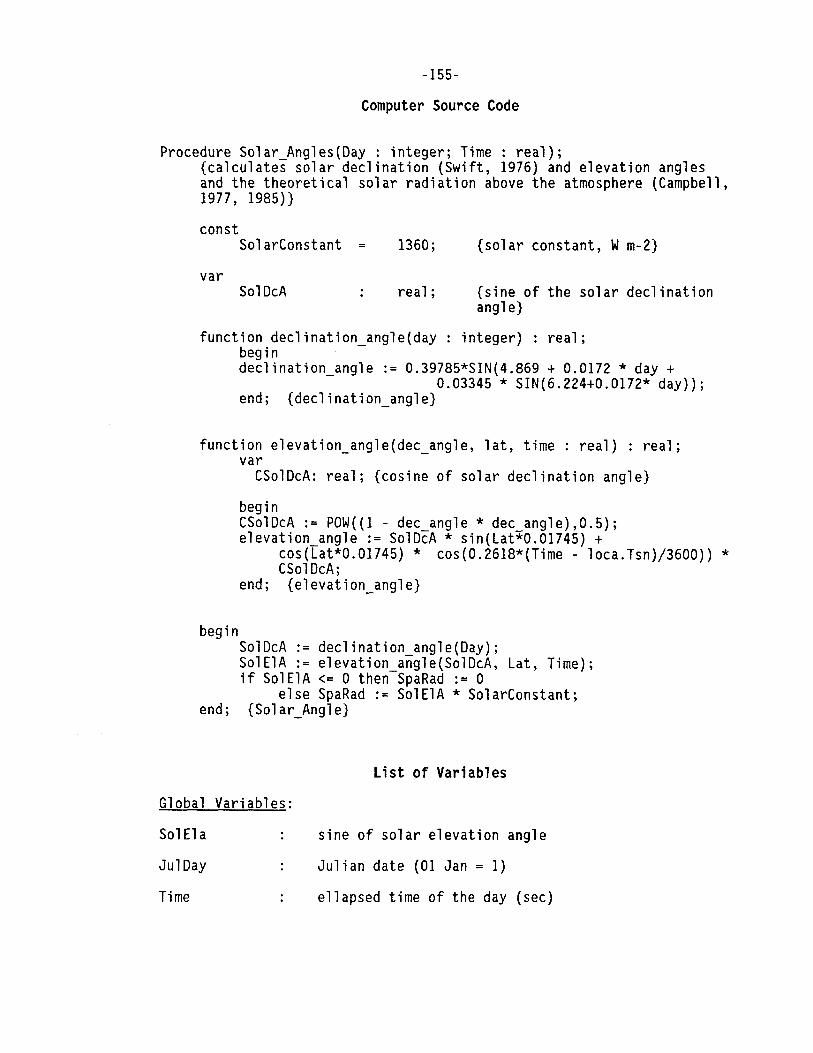
-155-

Computer Source Code

Procedure Solar_Angles(Day: integer; Time: real); {calculates solar declination (Swift, 1976) and elevation angles and the theoretical solar radiation above the atmosphere (Campbell, 1977, 1985))

canst SolarConstant =

var SolDcA

1360;

real;

{solar constant, W m-2)

{sine of the solar declination angle}

function declination angle(day integer) : real; begin -declination angle := 0.39785*SIN(4.869 + 0.0172 *day+

- 0.03345 * SIN(6.224+0.0172* day)); end; {declination angle}

function elevation_angle(dec_angle, lat, time : real) : real; var

begin

CSolDcA: real; {cosine of solar declination angle}

begin CSolDcA := POW((l - dee angle* dee angle),0.5); elevation_angle := SolDcA * sin(Lat*0.01745) +

cos(Lat*0.01745) * cos(0.2618*(Time - loca.Tsn)/3600)) * CSolDcA;

end; {elevation_angle}

SolDcA := declination_angle(Day); SolElA := elevation angle(SolDcA, Lat, Time); if SolElA <= O then-SpaRad := O

else SpaRad := SolElA * SolarConstant; end; {Solar_Angle}

Global Variables:

Sol Ela

JulDay

Time

List of Variables

sine of solar elevation angle

Julian date (01 Jan= 1)

ellapsed time of the day (sec)

Lat

Local Variables:

SolDcA

SpaRad

CSolDcA

Local Constants:

SolarConstant

-156-

latitude (degree)

sine of solar declination angle

hourly irradiance above the atmosphere (W m- 2 )

cosine of solar declination angle

solar constant (1360 w m- 2 )

3.2.2 Procedure Atmos Trans

The procedure Atmos Trans, called at the beginning of each day,

uses the daily theoretical solar radiation above the atmosphere

(SpaceSum), calculated once every day before entering the hourly loop

and the measured daily solar radiation (clim.SolRad) to arrive at an

estimate of fractional cloud cover and atmospheric transmission

coefficient. In other procedures (e.g. in Priestley_Taylor_ETP and

Penman ETP) these estimates are needed to calculate atmospheric

emissivity which will in turn be used to estimate longwave radiation.

The transmission coefficient {TTrans) of the atmosphere is simply

the ratio of measured to potential daily global solar radiation:

(1) TTrans = clim.SolRad / SolRad

where: clim.SolRad is the measured solar radiation

(MJ m- 2 d- 1 ) SolRad is the theoretical solar radiation (MJ m- 2 d- 1 )

-157-

Cloudiness or fractional cloud cover can be calculated as

(Campbell, 1985):

(2) Clouds= 2.33 - 3.33 * TTrans

and is valid only when Clouds has values between O and 1.

List of References

Campbell, G.S. 1985. Soil physics with BASIC. Elsevier, New York. 150 pp.


Procedure Atmos_Trans(day: integer);

var Sol Rad real; {theoretical solar radiation,MJ/m2/day}

begin SolRad := SpaceSum * 0.0864;

{converts W m-2 into MJ m-2 day-1} TTrans := climate.solar_rad[day].value / SolRad; Clouds:= 2.33-3.33*TTrans;

if Clouds< 0 then Clouds := O; if Clouds> l then Clouds := l;

end; {Atmos_Trans}

Global Variables:

Day

SpaceSum

clim.SolRad

Clouds

List of Variables

day number

theoretical solar radiation (W m-2)

measured solar radiation (MJ m-2 d-1)

fractional cloud cover

TTrans

atmosphere

Local Variables:

SolRad

-158-

total transmission coefficient for the

theoretical solar radiation (MJ m- 2 d- 1 )

Comment: multiplying by 0.0864 converts (W m- 2 ) into (MJ m- 2 d- 1 )

3.2.3 Procedure Air_Temperature

In the procedure Air_Temperature, daily values of minimum and

maximum measured air temperature are used to fit a sine function to

approximate values of air temperature at any hour during the day.

Maximum temperatures are assumed to occur at 1500 hours and minimum

temperatures at 300 hours. To assure smooth interpolation, the minimum

air temperature of the following day is used after 1500 hours, and the

maximum of the preceding day prior to 300 hours.

(1) AirTemp = 0.5 * (TempSum + TempDiff * COS(Angle))

where: TempSum is the sum of maximum and m1n1mum air temperature TempDiff is the difference between maximum and minimum air

temperature Angle is a function of time of day:

{2) Angle= 0.2618 * {Hour-15)

where Hour is the ellapsed hour of the day.

Minimum and maximum air temperatures are provided as input data in

the climate input file (Chp. 2.1.1). To obtain a constant air

temperature, simply set minimum temperature equal to maximum

temperature.

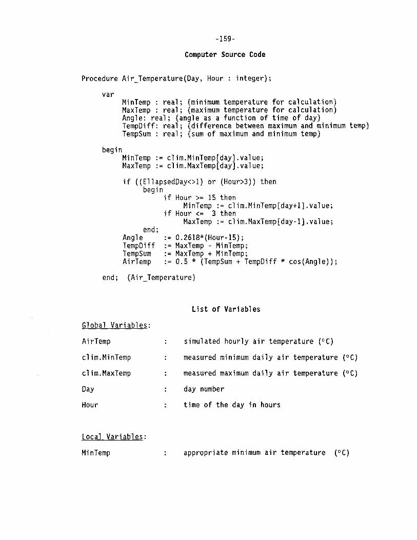
-159-


Procedure Air Temperature(Oay, Hour: integer);

var

begin

MinTemp : real; {minimum temperature for calculation} MaxTemp: real; {maximum temperature for calculation} Angle: real; {angle as a function of time of day} TempDiff: real; {difference between maximum and minimum temp} TempSum: real; {sum of maximum and minimum temp}

MinTemp := clim.MinTemp[day].value; MaxTemp := clim.MaxTemp[day].value;

if ((EllapsedOay<>l) or (Hour>3)) then begin

end; Angle TempDiff TempSum AirTemp

if Hour>= 15 then MinTemp := clim.MinTemp[day+l].value;

if Hour<= 3 then MaxTemp := clim.MaxTemp[day-1].value;

:= 0.2618*(Hour-15); := MaxTemp - MinTemp; := MaxTemp + MinTemp; := 0.5 * (TempSum + TempDiff * cos(Angle));

end; {Air Temperature}

Global Variables:

AirTemp

clim.MinTemp

clim.MaxTemp

Day

Hour

Local Variables:

MinTemp

List of Variables

simulated hourly air temperature (DC)

measured minimum daily air temperature (DC)

measured maximum daily air temperature (°C)

day number

time of the day in hours

appropriate minimum air temperature (DC)

MaxTemp

Angle

TempDiff

TempSum

-160-

appropriate maximum air temperature (°C)

angle as a function of time of day

difference between maximum and minimum air

temperature (°C)

sum of maximum and minimum air temperature (°C)

3.2.4 Procedure Priestley_Taylor_ETP

Priestley and Taylor (1972) developed an equation for calculating

potential evapotranspiration (ETP) for short vegetation, well-supplied

with water under nonadvective conditions. This equation incorporates a

proportionality factor known as the Priestley-Taylor factor (ALPHA) with

an expression for equilibrium evapotranspiration based on radiation.

The proportionality factor is supposed to compensate for the elimination

of the aerodynamic component from the Penman equation (see Penman_ETP,

3.2.5). Priestley and Taylor experimentally determined an average value

for ALPHA of 1.26, which is supported by the observation that the

radiation component is generally four to five times as large as the

aerodynamic component. An ALPHA very close to this value has since been

confirmed by several investigators (Stewart and Rouse, 1977; Davies and

Allen, 1973), when water supply to the evaporating surface is not a

limiting factor. To improve estimates under advective conditions

several attempts were made to estimate ALPHA from available climatic

data such as air temperature (Jury and Tanner, 1975) or air temperature

and net radiation (Nakayama and Nakamura, 1982). Others attempted to

correlate ALPHA with soil surface moisture (Davies and Allen, 1973).The

-161-

Priestley-Taylor equation has also been used to predict

evapotranspiration from forests (Shuttleworth and Calde, 1979).

Despite the empirical nature of the proportionality factor ALPHA,

the Priestley Taylor equation is based on reasonable physical grounds.

It reduces input data requirements and can be used in situations where

wind speed data and aerodynamic resistances are not available.

The Priestley-Taylor equation for potential evapotranspiration

(ETP) can be written as:

(1) sim.ETP = loca.ALPHA * (NetRad-G) * (SSVD/ (SSVD+PSYCON}} / LAMB

where: sim.ETP is the pot. evapotranspiration (kg m- 2 s- 1 ) loca.ALPHA is the Priestley-Taylor factor (1.08 - 1.34} NetRad is the net radiation (W m- 2) G is the soil heat flux (W m-2) SSVD is the slope of the saturation vapor density function (kg m- 3

k-1) PSYCON is the psychrometric constant (0.494 g m-3 K- 1 )

LAMB is the latent heat of vaporization of water (2450 J g-1, at 20 oc)

Net radiation (NetRad) is calculated as:

(2) NetRad = LWR + loca.AS * clim.SolRad * 11.574 * (SpaRad / SpaceSum)

where: LWR is net longwave radiation (W m- 2) loca.AS is the short wave absorptivity of the plant canopy or soil

surface (0.78) clim.SolRad is measured solar radiation (MJ m- 2 d- 1 ) being

converted to (W m- 2} by multiplication with 11.574 SpaRad is the theoretical solar radiation above the atmosphere for

a given time step (W m-2) SpaceSum is the theoretical solar radiation for a day (W/m2)

Net Lonqwave radiation (LWR) is calculated assuming the soil or plant surface is equal to air temperature:

(3) LWR = (EA - loca.ES) *ST* (AirTemp+273)A4

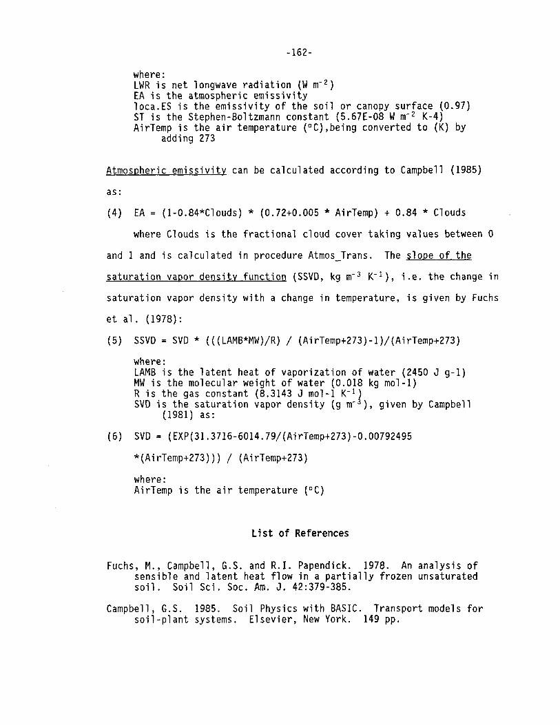
-162-

where: LWR is net longwave radiation (W m- 2 ) EA is the atmospheric emissivity loca.ES is the emissivity of the soil or canopy surface (0.97) ST is the Stephen-Boltzmann constant (5.67E-08 W m- 2 K-4) AirTemp is the air temperature (°C),being converted to (K) by

adding 273

Atmospheric emissivity can be calculated according to Campbell (1985)

as:

(4) EA= (l-0.84*Clouds) * (0.72+0.005 * AirTemp) + 0.84 * Clouds

where Clouds is the fractional cloud cover taking values between 0

and 1 and is calculated in procedure Atmos_Trans. The slope of the

saturation vapor density function (SSVD, kg m- 3 K- 1 ), i.e. the change in

saturation vapor density with a change in temperature, is given by Fuchs

et al. (1978):

(5) SSVD = SVD * (((LAMB*MW)/R) / (AirTemp+273)-1)/(AirTemp+273)

where: LAMB is the latent heat of vaporization of water (2450 J g-1) MW is the molecular weight of water (0.018 kg mol-1) R is the gas constant (8.3143 J mol-1 K- 1 ] SVD is the saturation vapor density (gm- ), given by Campbell

(1981) as:

(6) SVD = (EXP(31.3716-6014.79/(AirTemp+273)-0.00792495

*(AirTemp+273))) / (AirTemp+273)

where: AirTemp is the air temperature (°C)

List of References

Fuchs, M., Campbell, G.S. and R.I. Papendick. 1978. An analysis of sensible and latent heat flow in a partially frozen unsaturated soil. Soil Sci. Soc. Am. J. 42:379-385.

Campbell, G.S. 1985. Soil Physics with BASIC. Transport models for soil-plant systems. Elsevier, New York. 149 pp.

-163-

Davies, J.A. and C.D. Allen. 1973. Equilibrium, potential and actual evaporation from cropped surfaces in Southern Ontario. J. Appl. Meteorol. 12:649-657.

Jury, W.A. and C.B. Tanner. 1975. Advection modification of the Priestley-Taylor ET formula. Agron. J. 67:840-842.

Nakayama, K. and A. Nakamura. 1982. Estimating potential evapotranspiration by the Priestley-Taylor model. J. Agr. Met. 37:297-302.

Priestley, C.H.B. and B.J. Taylor. 1972. On the assessment of surface heat flux evaporation using large-scale parameters. Mon. Weather Rev. 100:81-92.

Sharma, M.L. 1985. Estimating Evapotranspiration. Advances in Irrigation 3:213-281.

Shuttleworth, W.J. and I.R. Calder. 1979. "Has the Priestley-Taylor equation any relevance to forest evaporation?" J. Appl. Meteorol. 18:639-646.

Stewart, R.B. and W.R. Rouse. 1977. Substantiation of the PriestleyTaylor parameter for potential evaporation in high latitude. J. Appl. Meteorol. 16:649-650.

Tanner, C.B. and W.A. Jury. 1976. Estimating evaporation and transpiration from a row crop during incomplete cover. Agron. J. 68:239-243.


-164-

Procedure Priestley_Taylor_ETP;

const PSYCON G

= 0.494; = 0.0;

{psychrometric constant, g m-3 K-1} {soil heat flux, W m-2}

var

begin

LAMB

ST MW R

EA LWR NetRad SSVD

SVD

= 2450.0; {latent heat of vaporization of water, J g-1}

= 5.67E-8;{Stephan-Boltzman constant, W m-2 K-4} = 0.018; {molecular weight of water, kg mol-1} = 8.3143; {gas constant, J mol-1 K-1)

rea 1; real; real; real;

real;

{atmospheric emissivity} {net longwave radiation, W m-2} {net radiation,W m-2} {slope of sat vapor density fct., kg m- 3

K- 1} {saturation vapor density, g m-3}

SVD := (EXP(31.3716-6014.79/(AirTemp+273) -0.00792495*(AirTemp+273))) /(AirTemp+273);

SSVD := SVD * (((LAMB*MW)/R)/(AirTemp+273)-1) / (AirTemp+273); EA := (1-0.84*Clouds) * (0.72 + 0.005*AirTemp) +

0.84*Clouds; LWR := (EA-loca.ES) *ST* POW((AirTemp+273.0),4.0); NetRad:= LWR + loca.AS * clim.SolRad[real day].value * 11.574

* (SpaRad/SpaceSum); -

sim.ETP:= loca.ALPHA * (NetRad-G) * (SSVD/(SSVD+PSYCON)) /(LAMB*lOOO);

if (clim.SolRad[real_day].value*(SpaRad/SpaceSum) = O) then sim.ETP := O;

if sim.ETP < 0 then sim.ETP := O;

end; {Priestley_Taylor_ETP}

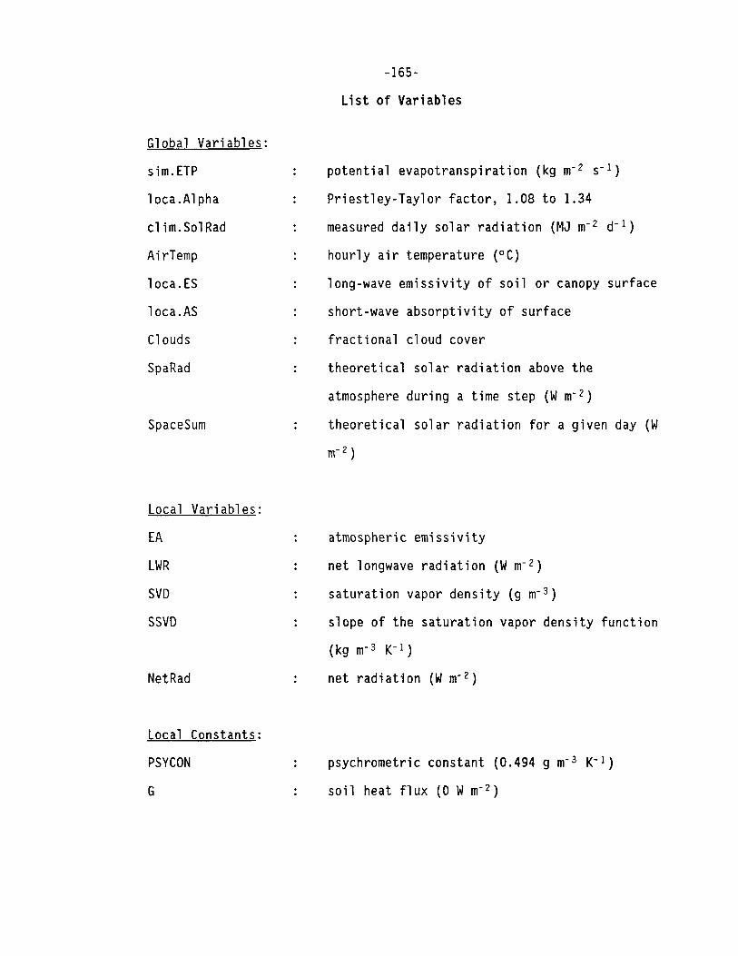
Global Variables:

sim. ETP

loca.Alpha

clim.SolRad

AirTemp

loca.ES

loca.AS

Clouds

SpaRad

SpaceSum

Local Variables:

EA

LWR

SVD

SSVD

NetRad

Local Constants:

PSYCON

G

-165-

List of Variables

potential evapotranspiration (kg m-2 s-1)

Priestley-Taylor factor, 1.08 to 1.34

measured daily solar radiation (MJ m- 2 d- 1 }

hourly air temperature (°C}

long-wave emissivity of soil or canopy surface

short-wave absorptivity of surface

fractional cloud cover

theoretical solar radiation above the

atmosphere during a time step (W m-2)

theoretical solar radiation for a given day (W

rn- 2 )

atmospheric emissivity

net longwave radiation (W m-2)

saturation vapor density (g m- 3}

slope of the saturation vapor density function

( kg m- 3 K- 1 }

net radiation (W m- 2}

psychrometric constant (0.494 g m-3 K-1)

soil heat flux (0 W m-2)

LAMB

ST

-166-

latent heat of vaporization of water (2450 Jg-

1, at 20 °C)

Stephan-Boltzman const. (5.67E-08 W m- 2 K-4)

3.2.5 Procedure Penman ETP

The Penman-Monteith equation combines a vapor diffusion and energy

budget approach to predict evapotranspiration from plant canopies.

Monteith (1964) applied the Penman equation (1948) to crop canopies,

arguing that the resistances to vapor diffusion from inside the leaves

through the stomates, leaf boundary layer and canopy, could be

incorporated into a single canopy resistance. Net radiation must be

known, change in soil heat storage either known or assumed to be

negligable, air temperature, relative humidity, and windspeed must be

known.

The procedure Penman ETP is divided into several smaller

procedures in order to apply the equation to both soil and cropped

surfaces. In the procedure Common, variables that are needed to predict

evapotranspiration from either soil surfaces or crop canopies are

calculated. First, the transmission coefficient of the canopy is

calculated as a function of the leaf area index of the crop from an

equation given by Stockle and Campbell (1985) and is subtracted from 1

in order to obtain the fraction of ETP allocated to transpiration.

TransFrac = 1 - ( exp( -0.823 *LAI+ 0.0286 * LAIA2))

where: LAI is the leaf area index (m2 m-2).

-167-

The saturation vapor density (SVD) is calculated as a function of air

temperature (Campbell 1985):

(1) SVD = (EXP(31.3716-6014.79 / (AirTemp+273)-0.00792495 * (AirTemp +

273))) / (AirTemp + 273)

where: SVD is the saturation vapor density (g m-3) AirTemp is air temperature (°C)

The slope of the saturation vapor density (SSVD) as a function of

temperature at a given temperature is calculated (Campbell 1985):

(2) SSVD = SVD * (((LAMB*MW)/R) /(AirTemp + 273} - 1/(AirTemp + 273)

where: SSVD is the slope of the saturation vapor density curve (g

m-3 K-1) LAMB is latent heat of vaporization (2430 J g-1) MW is molecular weight of water (18 g mole-I) R is the gasconstant (8.3143 J mole-1 K-1)

The actual vapor density (VD) is then calculated by multiplying the

relative humidity by the saturated vapor density.

(3) VD= clim.RelHumid[day] * SVD

where: VD is the vapor density of air (g m-3) SVD is the saturated vapor density of air (g m-3) clim.RelHumid is the relative humidity of the air

In the procedure Soil, variables in the Penman-Monteith equation

are determined assuming the surface of interest is a soil. First, the

aerodynamic resistance to vapor transfer (RA) for a soil surface is

calculated based on the theory of turbulent transport if a windspeed at

a specified height is known. For a soil surface, the zero plane

displacement (D) is assumend equal to Om. The momentum roughness

parameter (ZM) is assumed equal to 0.01 m. The vapor roughness

-168-

parameter (ZV) is assumed to be 20% of the height of the momentum

roughness parameter.

RA= (ln((loca.WindHeight - D + ZV) / ZV) * ln((loca.Windheight - D

+ ZM) / ZM )) / (KA2 * clim.Windspeed)

where: RA is the aerodynamic resistance to vapor transfer (s m-1) loca.Windheight is the height above soil surface at which

windspeed was measured (m) Dis the zero plane displacement (m) ZM is the momentum roughness parameter (0.01 m) ZV is the vapor roughness parameter (0.2 * ZM), K is the von Karman constant (0.4), clim.Windspeed is the measured windspeed (m s-1).

If windspeed is not known, the aerodynamic resistance to vapor

transport is assigned a constant value of 90 s m-1. Also in this

procedure, shortwave absorptivity (ABS) is assigned a value from the

soil input file.

In the next procedure, Crop, an areodynamic resistance for the

boundary layer abover the crop is calculated based on the same equation

used for calculating the aerodynamic resistance of the boundary layer

above a soil. However, in this case the height of zero plane

displacement is no longer zero but assumed to be 64% of the canopy

height (m). The momentum roughness parameter (ZM) is assumed to be 13%

of the canopy height and again the vapor roughness parameter (ZV) is

assumed to be 20% of ZM (Campbell 1977). If windspeed is not known,

then some assumed value for the aerodynamic resistance is called from

the plant input file. Within this procedure, the bulk canopy resistance

can either be assigned and held constant or can be made a function of

plant (leaf water potential), environmental (vapor density deficit) or

soil (soil water potential) factors, depending on the crop being

-169-

modelled. Shortwave absorptivity is assigned a value from the plant

input file.

The Penman-Monteith equation is applied in the procedure Penman.

First, net radiation (sim.NetRad) is calculated as the sum of absorbed

shortwave radiation and net longwave radiation.

sim.NetRad := LWR +ABS* clim.solrad[real_day].value *

11.574 * SpaRad/SpaceSum

where: LWR is net longwave radiation (W m-2) ABS is the shortwave absorptivity of the soil or crop clim.SolRad is solar radiation (MJ m-2 d-1) SpaRad is irradiance above the atmosphere (W m-2) SpaceSum is theoretical solar radiation for a day (W m-2) 11.574 converts MJ m-2 d-1 into W m-2

Next, latent heat of evapotranspiration (LE) is calculated:

LE=(SSVD*(sim.NetRadG)+(RO*(SVD-VD)/RA))/((PSYCON*(l+RC/RA))+SSVD)

where: LE is latent heat of evapotranspiration (J m-2 s-1) RO is the specific heat capacity of air (J m-3 K-1) RA is the canopy resistance to heat transport (s m-1) PSYCON is the psychrometric constant (g m-3 K-1) RC is the canopy resistance to vapor transport (s m-1) SSVD is the slope of the saturation vapor density curve (g m-3 K-1)

Latent heat of evapotranspiration is then converted into

evapotranspiration (sim.ETP) by dividing by the latent heat of

vaporization.

(5) sim.ETP =LE/ (LAMB* 1000}

where: LAMB is the latent heat of vaporization (2430 J kg-1) multiplication by 1000 converts g into kg

-170-

References

Campbell, G. S. 1985. Soil Physics with BASIC. New York: Elsevier.

Monteith, J. L. 1964. Evaportion and environment. In the State and Movement of Water in Living Organisms. 19th Symp. Soc. Exp. Biol.

Penman, H. L. 1948. Natural evaportion from open water bare soil and grass. Roy. Soc. London, Proc. Ser. A 193:120-146.


Procedure PenmanETP;

const

var

PSYCON= 0.494; RO = 1200.0; LAMB = 2430.0; R = 8.3243; MW = 18.0; ST = 5.67E-8; K = 0.4;

TransFrac: real; SVD real; SSVD real; VO real; EA real; LWR real; LE real;

RC RA D ZM zv ABS G

real; rea 1; real; real; real; real; real;

{psychometric constant, g m-3 K-1} {specific heat capacity of air,, J m-3 K-1} {latent heat of vaporization, J kg-1} {gas constant, J mole-1 K-1} {molecular weight of water, g mole-I} {Stephan-Boltzman constant, W m-2 K-4} {vonKarman constant}

{fraction of ETP allocated to transpiration} {saturation vapor density, g m-3} {slope of sat. vap. dens. curve, g m-3 K-1} {actual vapor density of air, g m-3) {atmospheric emissivity} {net longwave radiation, W m-2} {latent heat of evapotranspiration, J m-2 s-1}

{canopy resistance, s m-1) {aerodynamic resistance, s m-1} {zero plane displacement, m} {momentum roughness parameter, m} {vapor roughness parameter, m} {shortwave absorptivity} {soil heat flux, W m-2}

Procedure Common; {Calculates variables for P.M. equation common to soil and plant canopies}

begin TransFrac := 1 - exp(-0.823 *LAI+ 0.286 * LAIA2);

SVD ·.- (EXP(31.3716-6014.79/(AirTemp+273) -0.00792495*(AirTemp+273))) / (AirTemp+273);

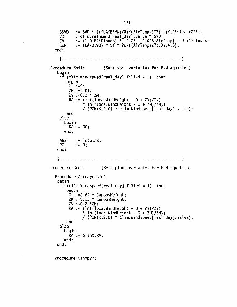
-171-

SSVD VD EA LWR

:= SVD * (((LAMB*MW)/R)/(AirTemp+273)-1}/(AirTemp+273}; :=clim.relhumid[real day].value * SVD; := (1-0.84*Clouds) *-(0.72 + O.OOS*AirTemp) + 0.84*Clouds; := {EA-0.98} *ST* POW((AirTemp+273.0},4.0};

end;

{----------------------------------------------------} Procedure Soil; {Sets soil variables for P-M equation}

begin if (clim.Windspeed[real day].filled = 1} then

begin -D : =0; ZM :=0.01; ZV :=0.2 * ZM; RA:= (ln((loca.WindHeight - D + ZV)/ZV)

* ln((loca.WindHeight - D + ZM}/ZM}} / (POW(K,2.0) * clim.Windspeed[real_day].value);

end else

begin RA:= 90;

end;

ABS := loca.AS; RC : = 0;

end;

{-----------------------------------------------------}

Procedure Crop; {Sets plant variables for P-M equation}

Procedure AerodynamicR; begin if (clim.Windspeed[real day].filled = 1) then

begin -D :=0.64 * CanopyHeight; ZM :=0.13 * CanopyHeight; ZV :=0.2 *ZM; RA:= (ln((loca.WindHeight - D + ZV)/ZV)

* ln((loca.WindHeight - D + ZM)/ZM)) / (POW(K,2.0) * clim.Windspeed[real day].value};

end else

begin RA:= plant.RA;

end; end;

Procedure CanopyR;

-172-

begi n RC := plant.Reopen; if RC< plant.Reopen then RC:=plant.RCopen;

end;

begin

ABS :=plant.AS; AerodynamicR; CanopyR;

end;

{-----------------------------------------------------) Procedure Penman; {Calculates Penman.ETP)

begin

if (clim.solrad[real_day].value*(SpaRad/SpaceSum)=O) then sim.ETP:=0

end;

else begin

sim.NetRad := (LWR +ABS* clim.solrad[real day].value * 11.574 * SpaRad/SpaceSum) --G;

G := 0.10 * sim.NetRad; LE := (SSVD*(sim.NetRad-G)+(RO*(SVD-VD)/RA)) /

((PSYCON*(l.O+RC/RA))+SSVD); sim.ETP:= LE/(LAMB*lOOO); if sim.ETP<O then sim.ETP:=0;

end;

{-----------------------------------------------------} begin

end;

CanopyHeight:=plant.CanopyHeight; RA := plant.RA; Common; Soi 1 ; Penman; sim.POTEVA := sim.ETP*(l.0-TransFrac); if there is a plant then Crop; if there-is-a-plant then Penman; sim.POTTRANS := sim.ETP*Transfrac; sim.ETP:=sim.POTTRANS + sim.POTEVA;

Global Variables:

sim.ETP

AirTemp

clim.RelHumid

clim.SolRad

SpaRad

SpaceSum

loca.AS

loca.RT

loca.RV

Local Variables:

SVD

SSVD

VD

LE

G

Local Constants:

PSYCON

RO

LAMB

-173-

List of Variables


air temperature (°C)

relative humidity

Measured daily solar radiation (MJ m-2 d-1)

irradiance above the atmosphere (W m-2)

theoretical solar radiation for a given day (W m-2)

short-wave absorptivity of the surface

resistance to heat transport (s m-1)

resistance to vapor transport (s m-1)

saturation vapor density (g m-3)

slope of sat. vap. dens. curve (g m-3 K-1)

actual vapor density of air (g m-3)

latent heat of evapotranspiration (J m-2 s-1)

soil heat flux (W m-2)

psychometric constant, 0.494 g m-3 K-1

specific heat capacity of air, 1200 J m-3 K-1

latent heat of vaporization, 2430 J kg-1

MW

R

-174-

molecular weight of water, 18 g mole-I

gas constant, 8.3143 J mole-I K-1

3.2.6 Procedure Pan ETP

The procedure Pan_ETP uses daily measured values for pan

evaporation provided in the climate input file (clim.PanEV) and

distributes the evaporative demand during the day using a sine wave

function. A pan coefficient (loca.Kp) and a crop coefficient (loca.Kc)

can be specified in the location input file.


Procedure Pan_ETP;

begin sim.ETP:= 2.3 * clim.PanEV[real day].value

* {0.05 + POW{SIN(0.0175*7.5 * ellapsed hour),4)) / 86400.0 * loca.Kc * loca.Kp; -

if SpaRad <= 0 then sim.ETP := O; end;

Global Variables:

sim.ETP

clim.PanEV

real_day

ellapsed hour

loca.Kc

List of Variables


measured pan evaporation (mm d-1)

day number

ellapsed hour

crop coefficient

loca.Kp

SpaRad

-175-

pan coefficient

theoretical solar radiation above the

atmosphere during a time step (W m- 2 )

3.2.7 Linacre ETP

The procedure Linacre ETP uses a simple empirical formula (Linacre,

1977) to estimate potential evapotranspiration from mean daily air

temperature, mean daily dew-point temperature, elevation and latitude.

If dew-point temperature is unavailable, minimum daily temperature can

be used as an approximation.

The daily mean air temperature (TMean) is calculated as:

TMean := (clim.MinTemp[real_day].value +

clim.MaxTemp[real day].value) / 2;

where: clim.MinTemp is the measured daily minimum air temperature clim.MaxTemp is the measured daily maximum temperature

Daily potential evaporation (ETPdaily) is calculated as:

ETPdaily:= (700 * Tm/(100 - loca.latitude) + 15*(TMean-Td)) /

(80-TMean);

where: Tm equals TMean + 0.006 * loca.elevation Td is the dew-point temperature loca.latitude is latitude TMean is mean temperature (°C)

The daily evaporative demand is then distributed over the day using a

sine function. The instantaneous rate of potential evapotranspiration

(sim.ETP) is:

sim.ETP := 2.3 * ETPdaily * (0.05 + POW(SIN(0.0175*7.5 *

ellapsed_hour),4)) / 86400.0;

-176-

where: ellapsed_hour is the ellapsed time in a day (hours)

If the sine of the solar elevation angle is less than 0, sim.ETP is

set equal to 0. The potential evapotranspiration (sim.ETP) is

partitioned into potential evaporation (sim.PotEva) and potential

transpiration (sim.PotTrans) according according to Stockle and Campbell

(1985):

TransFrac := 1 - exp(-0.823 *LAI+ 0.286 *LAI* LAI);

sim.PotTrans := sim.ETP*Transfrac;

sim.PotEva := sim.ETP*(l.0-TransFrac);

where: LAI is the leaf area index

References

Linacre, E.T. 1977. A simple formula for estimating evaporation rates in various climates, using temperature data alone. Agric. Meteorol. 18:409-424.

Procedure Linacre_ETP;

var Tm TMean Td ETPdai ly TransFrac

begin

real; real; real; real; real;


{empirical parameter} {mean daily air temperature} {mean dewpoint temperature} {potential evapotranspiration, mm day-1) {fraction of ETP allocated to transpiration}

TMean := (clim.MinTemp[real day].value + clim.MaxTemp[real day].value) / 2;

Tm:= TMean + 0.006 * loca.elevation; Td := clim.MinTemp[real day].value; ETPdaily:= (700 * Tm/(100 - loca.latitude) + 15*(TMean-Td)) /

(80-TMean);

-177-

s im. ETP := 2.3 * ETPdaily * (0.05 + POW(SIN(0.0175*7.5 * ellapsed_hour),4)) / 86400.0;

if SolElA <= 0 then sim.ETP := O;

TransFrac := 1 - exp(-0.823 *LAI+ 0.286 *LAI* LAI);

sim.POTTRANS .- sim.ETP*Transfrac; sim.POTEVA .- sim.ETP*(l.0-TransFrac);

end;

Global Variables:

sim.ETP

sim.PotTrans

sim.PotEva

clim.MinTemp

clim.MaxTemp

loca.elevation

l oca. latitude

Local Variables:

Tm

TMean

Td

ETPdaily

TransFrac

List of Variables


potential transpiration (kg m-2 s-1)

potential soil evaporation (kg m-2 s-1)

measured minimum air temperature (°C)

measured maximum air temperature (°C)

elevation (m)

latitude (degrees)

empirical parameter

mean daily air temperature (°C)

mean dewpoint temperature (°C)

potential evapotranspiration {mm day-1)

fraction of ETP allocated to

transpiration}

-178-

3.2.8 Procedure Max Photosynthesis

The procedure Max_PhotoSynthesis is from a simulation model

developed by Stockle and Campbell {1985} to predict the effects of water

stress on corn yield. It is called on an hourly basis and implemented

whenever there is daylight {sine of the Solar Elevation Angle is greater

than O}. At night, photosynthesis is assumed to equal O and the

stomatal resistance is set at a high value representative of closed

stomates (3200 s m-1). During the day, photosynthesis is calculated as

a function of photosynthetically active radiation and leaf temperature.

This procedure also calculates a non-stressed canopy resistance to water

vapor loss based on the maximum stomatal resistance required to achieve

the predicted photosynthesis rate, assuming that internal leaf CO2

concentration, ambient CO2 concentration and the boundary layer

resistance to CO2 are known or can be estimated. As written, this

procedure can only be applied to homogeneous plant canopies and not to

mixed plantings or isolated plants.

This procedure begins by determining the amount of leaf area that

is sunlit. An extinction coefficient (K} for a spherical (random) leaf

angle distribtion is calculated as a function of the sine of the solar

elevation angle.

(I) K = 0.5 / SolElA

where:

SolElA is the sine of the solar elevation angle

This equation, as well as others for calculating extinction coefficients

for different types of leaf inclination angles, is presented and

discussed in Campbell (1977). The sunlit leaf area index (LAISun) is

-179-

then calculated as a function of the total leaf area and extinction

coefficient.

(2) LAISun = (1 - EXP(-K *LAI))/ K

where:

LAI is the leaf area index (m2 leaves m-2 ground), K is the canopy extinction coefficient.

The shaded leaf area index (LAIShade) is the difference between the

total leaf and the sunlit leaf area (LAIShade = LAI - LAISun).

In the next section of the procedure direct and diffuse

photosynthetically active radiation (PAR) is calculated. First, PAR is

calculated from solar radiation assuming half of the short wave spectrum

is PAR.

(3) PAR= 0.5 * (clim.SolRad[real day].value * 11.574 SpaRad /

SpaceSum)

where: clim.SolRad is measured daily solar radiation (MJ m-2 d-1) SpaRad is the theoretical solar radiation above the atmosphere

during a time step (W m-2) SpaceSum is the theoretical solar radiation for a given day (W m-2)

PAR for sunlit leaves (PARSun) is assumed to be a function of the

proportion of the total transmission coefficient of the atmosphere

(TTrans) that is direct radiation (1-0Trans/TTrans) multiplied by the

canopy extinction coefficient (K) plus the proportion of the total

transmission coefficient of the atmosphere that is diffuse radiation

(DTrans/TTRans) (Norman 1982).

(4) PARSun = PAR (K * (1 - DTrans / TTrans) + DTrans / Trans)

where: PAR is photosynthetically active radiation (W m-2), K is the canopy extinction coefficient,

-180-

DTrans is the diffuse transmission coefficient of the atmosphere,

TTrans is the total transmission coefficient of the atmosphere.

PAR for shadelit leaves {PARShade) is calculated as a function of the

proportion of the total transmission coefficient of the atmosphere that

is the diffuse radiation coefficient multiplied by diffuse transmission

coefficient of the canopy {Kd) plus the scattered irradiance within the

canopy {Scirr) {Norman 1982).

{5) PARShade =PAR* Kd * DTrans / TTrans + Sclrr

where: PAR is the photosynthetically active radiation {W m-2) Kd is the diffuse transmission coefficient for the canopy DTrans is the diffuse transmission coefficient for the atmosphere TTrans is the total transmission coefficient for the atmosphere Sclrr is scattered radiation

Scattered irradiance is estimated as:

{6) Sclrr = {1-DTrans/TTrans) *PAR* 0.07 * {1.1-0.l*LAI) * EXP{-

SolElA)

where: DTrans is diffuse transmission coefficient of the atmosphere TTrans is total transmission coefficient of the atmosphere PAR is photosynthetically active radiation (W m-2) LAI is leaf area index SolElA is sine of solar elevation angle

Both sunlit (PSSun) and a shadelit {PSShade) rates of

photosynthesis are then calculated assuming that photosynthesis is

related to PAR according to an equation given for corn by Hesketh and

Baker {1969). This rate is then modified for canopy temperature

{assuming the leaf temperature equals air temperature) based on an

equation from Stockle and Campbell (1985) derived from data of Hofstra

and Hesketh (1969). To model photosynthesis for another crop, these

-181-

equations would have to be replaced by the appropriate functions for the

crop of interest.

(7) TempFac = -1.37893 + 0.184573*LeafTemp - 7.6341E-03 *

POW(LeafTemp,2) + l.98485E-04 * Pow(LeafTemp,3)

2.15152E-06 * POW(LeafTemp,4);

where: LeafTemp is the leaf temperature (°C)

(8) PSSun = 6.2527E-05 * POW(PARSun,0.507578) * TempFac / 0.7;

where: PARSun is photosynthetically active radiation for sunlit LAI (Wm-

2) TempFac is temperature function for photosynthesis

(9) PSShade = 6.2527E-05 * POW(PARShade,0.507578) * TempFac / 0.7;

where: PARShade is photosynthetically active radiation for shaded LAI (W m-2) TempFac is temperature function for photosynthesis

Crop photosynthesis for the hour (PS) is then obtained by multiplying

the photosynthetic rate for sunlit leaves (PSSun) by the sunlit leaf

area index (LAISun} and adding to this the photosynthetic rate for

shaded leaves (PSShade) multiplied by the shaded leaf area index

(LAIShade).

(10) PS= (PSSun*LAISun + PSShade*LAIShade) * time_step;

where: PSSun is photosynthetic rate of sunlit LAI (g m-2 s-1) LAISun is sunlit leaf area index PSShade is photosynthetic rate of shaded LAI (g m-2 s-1) LAIShade is shaded leaf area index time_step is the time step (s)

In the final section of the code, a "non-stressed" stomatal

resistance to vapor loss is calculated for both shaded and sunlit

leaves. This is accomplished by using Ohm's equation to model CO2

-182-

diffusion from the atmosphere into the leaves (PS= (COext-COint)/(RACO

+ RESCO)). This equation is rearranged to solve for RES and also

divided by 1.65 to convert from CO2 to water vapor resistance (Campbell

1977).

ResSun = ((COext - COint) / PSSun - RaCO) / 1.65

ResShade = ((COext - COint / PSShade - RaCO) / 1.65

where: ResSun is the sunlit stomatal resistance to water vapor

transfer (s m-1), ResShade is the shadelit stomatal resistance to water vapor

transfer (s m-1), COext is the atmospheric CO2 concentration (0.54 g m-3), COint is the CO2 concentration internal to the leaf (assumed

here to be 0.20 g m-3), RaCO is the leaf boundary layer resistance to CO2 transfer, PSSun is the photosynthesis rate of sunlit leaves (g m-2 s-1), PSShade is the photosynthesis rate of shadelit leaves (g m-2 s-1).

To then obtain the whole canopy non-stress resistance to water vapor

transfer the sun and shade lit resistances are weighted according to the

proportion of sun and shade lit leaf area and added in parallel (Stockle

and Campbell 1985).

NonStressRes =LAI/ (LAISun / ResSun + LAIShade / ResShade)

This an optimization approach to predicting water vapor loss from a

plant canopy since there is an implicit assumption that the plant only

opens its stomates the amount necessary to achieve maximum

photosynthesis and is never losing more water than required to achieve

this rate.

List of References


-183-

Hesketh, J. and D. Baker. 1967. Light and carbon assimilation by plant communities. Crop Sci. 7:285-293.

Hofstra, G. and J. D. Hesketh. 1969. Effect of temperature on the gas exchange of leaves in the light and dark. Planta 85:228-237.

Norman, J.M. 1982. Simulation of microclimates. "Biometeorology in integrated pest management". Academic Press, New York.

Stockle, C., and G. S. Campbell. 1985. A simulation model for predicting effect of water stress on yield: an example using corn. Adv. in Irrigation 3:283-323.


Procedure Max Photosynthesis; {Light and temperature limited}

canst COext COint RACO

var LAISun LAIShade PSSun

PSShade

K Kd

LeafTemp TempFac PAR

Scirr PARSun

PARShade

ResSun

ResShade

begin

= 0.54; 0.20; 100.0;

real; real; real;

rea 1;

real; real;

real; real; real;

real; real;

real;

real;

real;

if SolElA <= 0 then begin

{external CO2 concentration, g m-3) {internal CO2 concentration, g m-3) {boundary layer resistance for CO2 tranfer, s m-1)

{sunlit leaf area index} {shaded leaf area index} {photosynthetic rate of sumlit LAI, g m-2 s-1)

(photosynthetic rate of shaded LAI, g m-2 s-1)

{canopy extinction coefficient} {diffuse transmission coefficient for the canopy)

{leaf temperature, °C} {temperature fct for photosynthesis} {photosynthetically active radiation, W m-2)

{scattered irradiance, W m-2) {photosynthetically active radiation for sumlit LAI, W m-2)

{photosynthetically active radiation for shaded LAI, W m-2)

{non-stress stomatal resistance for sunlit leaves, s m-1)

{non-stress stomatal resistance for shaded leaves, s m-1)

-184-

PS:=0; NonStressRes:=3200; {stomates shut}

end

else begin K Kd

:= 0.5 / SolElA; := I - exp{-0.823 *LAI+ 0.0286 *LAI* LAI);

{calculate shaded and sunlit LAis} LAISun := {1-EXP{-K *LAI))/ K; LAIShade := LAI - LAISun; PAR := 0.5 * {clim.SolRad[real day].value * 11.574 *

SpaRad/SpaceSum); -PARSun :=PAR* {K*{l- DTrans/TTrans)+DTrans/TTRans); PARShade :=PAR* Kd * DTrans/TTrans + Scirr;

{calculate shade and sunlit PAR} Scirr := {1-DTrans/TTRans) *PAR* 0.07

* {1.1-0.l*LAI) * EXP{-SolElA); LeafTemp:= AirTemp; Tempfac := -1.37893 + 0.184573*LeafTemp - 7.6341E-03 *

POW(LeafTemp,2) + l.98485E-04 * Pow{LeafTemp,3) -2.15152E-06 * POW{LeafTemp,4);

{calculate shade and sunlit photosynthetic rates and stomatal resistances}

PSSun := 6.2527E-05 * POW{PARSun,0.507578) * Tempfac / 0.7; PSShade := 6.2527E-05 * POW(PARShade,0.507578) * Tempfac / 0.7; PS := {PSSun*LAISun + PSShade*LAIShade) * time step;

ResSun := {{COext - Coint) / PSSun - RACo)/1.65; ResShade := {(COext - Coint) / PSShade - RACo)/1.65;

NonStressRes:= LAI/ {LAISun / ResSun + LAIShade / ResShade); end;

end; {Max_Photosynthesis}

Global Variables:

SolElA

PS

List of Variables

sine of solar elevation angle

photosynthesis {g m-2 hour-I)

NonStressRes:

AirTemp

cl im. Sol Rad:

SpaRad

SpaceSum

LAI

DTrans

TTrans

Local Variables:

LAISun

LAIShade

PSSun

PSShade

K

LeafTemp

TempFac

PAR

Scirr

PARSun

PARShade

ResSun

-185-

non-water-stressed stomatal resistance (s m-1)

air temperature (DC)

measured solar radiation (MJ m-2 day-1)

theoretical solar radiation above the atmosphere

during a time step (W m-2)

theoretical solar radiation for a given day (W m-2)

Leaf area index

diffuse transmission coefficient of the atmosphere

total transmission coefficient of the atmosphere

sunlit leaf area index

shaded leaf area index

photosynthetic rate of sumlit LAI (g m-2 s-1)

photosynthetic rate of shaded LAI (g m-2 s-1)

canopy extinction coefficient

leaf temperature (DC)

temperature fct for photosynthesis

photosynthetically active radiation (W rn-2)

scattered irradiance (W m-2)

photosynthetically active radiation

for surnlit LAI (W m-2)

photosynthetically active radiation

for shaded LAI (W m-2)

non-stress stomatal resistance

for sunlit leaves (s m-1)

ResShade

Local Constants:

COext

COint

RACO

-186-

non-stress stomatal resistance

for shaded leaves (s m-1)

external CO2 concentration (0.54 g m-3)

internal CO2 concentration (0.20 g m-3)

boundary layer resistance for CO2 tranfer (100 s

m-1)

3.2.9 Procedure Critical Leaf Water Potential - - -The procedure Critical_Leaf_Water_Potential is from a simulation

model developed by Stockle and Campbell (1985} to predict the effects of

water stress on corn yield. It can be called on an hourly basis

whenever the simulated potential transpiration (sim.PotTrans} is greater

than 0. This procedure uses an empirically derived equation that

relates decreases in leaf water potentials to increases in stomatal

resistance. The increase in stomatal resistance contributes to a

simulated decrease in actual transpiration (ActTrans} below potential

transpiration. Using Ohm's Law to model water flow through plants

[ActTrans = (RootWP - LeafWP) / LeafRes] a new leaf water potential

(LeafWP) based on the simulated actual transpiration is calculated.

This leaf water potential, in turn, is used to calculate a new stomatal

resistance, which then results in a new simulated ActTrans and LeafWP.

This process is repeated until LeafWP changes less than 10 J kg-1 with

successive iterations.

-187-

Initially, the saturation vapor density (SVD, g m-3) is calculated

according to Campbell (1981) and the slope of the saturation vapor

density function (SSVD, g m-3 K-1) is calculated according to Fuchs et

al. (1978).

SVD = (EXP(31.3716-6014.79/(AirTemp+273)-

0.00792495*(AirTemp+273)))/(AirTemp+273)

where: AirTemp is the air temperature (°C) SSVD = SVD * (((LAMB*MW/R) / (AirTemp+273)-1)/(AirTemp+273) where: LAMB is the latent heat of water vaporization (2450 J g-1), MW is the molecular weight of water (2450 J g-1), R is the gas constant (8.3143 J mol-1 K-1)

The stressed stomatal resistance (StressRes) is calculated next

based on the work of Fisher et al. (1981) using values for corn given by

Stockle and Campbell (1985).

StressRes = NonStressRes * (1 + (LeafWP /

plant.CriticalleafWP)Aplant.S)

where: NonStressRes is the non-stressed stomatal resistance

calculated in the procedure Max_Photosynthesis (s m-1), LeafWP is the simulated LeafWP calculated in the procedure

Water Uptake (J kg-1), plant.CritTcalleafWP is a species dependent, empirically

derived value (J kg-1), plant.Sis a species dependent, empirically derived constant.

The reduction in transpiration that occurs due to an increase in

stomatal resistance is related to the contribution of stomatal

resistance to the total resistance to vapor transport given by Campbell

(1977). The ratio of non-stressed to stressed resistances (F) is

calculated and this term is then multipled by potential transpiration

(sim.PotTrans) to give actual transpiration (ActTrans).

-188-

F (SSVD + PSCON * (NonStressRes + plant.RA)/Re) / (SSVD +

PSYCON * {StressRes + plant.RA)/Re)

where: SSVD is the slope of the saturation vapor density function (g m-3

K-1), PSYCON is the psychrometric constant (0.494 g m-3 K-1), Plant.RA is the crop boundary layer resistance (s m-1), Re is the combined resistance for convection and longwave

radiation heat transfer (s m-1).

After calculating simulated actual transpiration (ActTrans = F *

sim.PotTrans) a new simulated leaf water potential (LeafWP) is

calculated.

LeafWP = RootWP - ActTrans * LeafRes

where: RootWP is the root water potential calculated in the

procedure Water Uptake (J kg-1), LeafRes is the leaf resistance to liquid water transport (m4 s-1

kg-1) assumed equal to 2 x JQA6 (Campbell 1985).

The hourly photosynthetic rate (PS) is also reduced as a function of the

stressed stomatal resistance (PS= F*PS).

In this last section of this procedure, a stress factor which

affects leaf area index development is calculated if actual

transpiration is less than 90% of potential transpiration.

LAIStressFact = LAIStressFact + sim.PotTrans/ActTrans*0.8

The transpiration deficit is accumulated on an hourly basis and

used outside this procedure to calculate a stress index.

Stress= 1 - ActTrans/sim.PotTrans

References


-189-

Campbell, G.S. 1981. Fundamentals of radiation and temperature relations. Physiological Plant Ecology I. Encyclop. Plant Physiol., New Ser. 12A.

Fisher, M. J., Charles-Edwards, D. A., and M. M. Ludlow. 1981. An analysis of the effects of repeated short term soil water deficits on stomatal conductance to carbon dioxide and leaf photosynthesis by the legume Macroptilium atropurpureum cv. Siratro. Aust. J. Plant Physiol. 8:347-357.

Fuchs, M., Campbell, G.S. and R.I. Papendick. 1978. An analysis of sensible and latent heat flow in a partially frozen unsaturated soil. Soil Sci. Soc. Am. J. 42:379-385.

Stockle, C., and G. S. Campbell. 1985. A simulation model for predicting effect of water stress on yield: an example using corn. Adv. in Irrigation 3:283-323.

-190-


Procedure Critical Leaf_Water_Potential;

const LAMB R

= 2430.0; = 8.3243; = 18.0;

{latent heat of vaporization, J kg-1}

MW Re 40;

PSYCON = 0.494; LeafRes 2E+06;

var SVD real; SSVD : real; StressRes: real ;

I LastLWP DeltaLWP

: integer; real; real;

{gas constant, J mole-I K-1} {molecular weight of water, g mole-I} {combined resistance for convective and LWR

heat transfer, s m-1}

{saturation vapor density, g m-3} {slope of sat. vap. dens. curve, g m-3 K-1} {stomatal response as a fct of leaf water

potential} {counter variable}

begin SVD ·.- (EXP(31.3716-6014.79/(AirTemp+273) - 0.00792495 *

(AirTemp+273))) / (AirTemp+273); SSVD := SVO * (((LAMB*MW)/R) /(AirTemp+273)-l)/(AirTemp+273);

Repeat StressRes:= NonStressRes * (l+ POW((LeafWP /

plant.CriticalleafWP),plant.S)); LastLWP:=LeafWP; F:= (SSVD + PSYCON * (NonStressRes + plant.RA)/Re) /

(SSVD + PSYCON * (StressRes + plant.RA)/Re); ActTrans := F * sim.PotTrans; LeafWP := RootWP - ActTrans * LeafRes; DeltaLWP:= ABS(LeafWP-LastLWP);

until DeltaLWP < 10;

PS:= PS* F;

if sim.PotTrans > 0 then begin

Stress:= (1 - ActTrans / sim.PotTrans); if (ActTrans/sim.PotTrans) < 0.9 then

LAIStressFact:= LAIStressFact + sim.PotTrans / ActTrans * 0.8; end;

end; {Critical_Leaf_Water_Potential}

Global Variables:

PS

F

AirTemp

NonStressRes

LeafWP

plant.CriticalleafWP:

plant.S

plant.RA

ActTrans

sim.PotTrans

RootWP

Stress

LAIStressFact

Local Variables:

-191-

List of Variables

photosynthesis (g CO2 m-2 hour-1)

ratio of nonstressed to stressed

resistances

air temperature {°C)

non-stressed stornatal resistance {s m-1)

leaf water potential (J kg-1)

crop dependent parameter (J kg-1)

crop dependent parameter

boundary layer resistance (s m-1)

actual transpiration (kg m-2 s-1)


root water potential (J kg-1)

hourly relative transpiration deficit

stress index for leaf area development

SVD saturation vapor density (g m-3)

SSVD slope of sat. vap. dens. curve (g m-3 K-1)

StressRes: stornatal response as a fct of leaf water potential

LastLWP leaf water potential of last time step (J kg-1)

DeltaLWP

I

Local Constants:

LAMB

R

MW

Re

PSYCON

LeafRes

plant.S

-192-

change in leaf water potential over one time step (J

kg-1)

counter variable

latent heat of vaporization (2430.0 J kg-1)

gas constant (8.3243 J mole-I K-1)

molecular weight of water (18.0 g mole-I)

combined resistance for convective and LWR

heat transfer (40 s m-1)

psychrometric constant (0.494 g m-3 K-1)

leaf mesophyll resistance to liquid flow (2E+06 m4

s-1 kg-I)

crop specific constant

-193-

3.2.10 Growth Stages


Procedure Growth_Stages;

var TMean DD Tl, T2

begin

real; real; real;

{mean daily air temperature} {degree days} {upper and lower limits of air temperature for growing degree day calculations}

TMean := (clim.MinTemp[real day].value + clim.MaxTemp[real_day].value) / 2.0;

If (TMean >= 6.0) and (TMean < 21.0) then DD:= 0.027 * TMean - 0.162;

If (TMean >= 21.0) and (TMean < 28.0) then DD:= 0.086 * TMean - 1.41;

If (TMean >= 28.0) and (TMean < 32.0) then DD := 1.0;

If (TMean >= 32.0) and (TMean < 44.0) then DD:= -0.083 * TMean +3.67;

If {TMean >= 44.0) or (TMean < 6.0) then DD:= O;

AccDD := AccDD + DD;

T2 := clim.MaxTemp[real day].value; Tl := clim.MinTemp[real-day].value; if T2 > 30 then T2 := 30; if Tl< 10 then Tl := 10; GDD := GDD + ((Tl+T2)/2) - 10;

end;

-194-

3.2.11 Dry_Matter_Accumulation


Procedure Dry_Matter_Accumulation;

var DAE : PartFactor: PartRatio DryMatter

LAR

integer; real; real; real;

real;

MaxRootingDepth: real;

procedure Root Growth; var I : integer; begin

{days after emergence} {factor for partitioning} {shoot/root partitioning} {dry matter accumulation rate, kg m-2 day-I}

{leaf area ratio, m2 leaf area kg-1 dry matter}

for I:= plant.FRoot to soil.Lastlayer do begin if (RootingDepth / 100) >= LowBound[I]

then plant.NRoot := I+l; end;

if plant.NRoot <= plant.FRoot then plant.NRoot:=Plant.FRoot; if plant.NRoot >= 8 then plant.NRoot:= 8;

end;

begin {calculate partitioning} MaxRootingDepth := plant.MaxRootDepth; DAE := Real day - Plant.EmergenceDate; If DAE< SO-then PartFactor := 0.125 * DAE; If DAE< 16 then PartFactor := 2; If DAE >=50 then PartFactor := 0.135 * DAE; PartRatio := PartFactor / (PartFactor+l);

{dry matter production} DryMatter:= 0.40 * (SumPS / 1000.0); if AccDD >= 33 then DryMatter:= 0.33 * (SumPS / 1000.0); {after

pollination if AccDD >= 49

then DryMatter:=0 {after maturation}

{dry matter accumulation} AccTotalDryMatter := AccTotalDryMatter + DryMatter; AccTopDryMatter := AccTopDryMatter + DryMatter * PartRatio; AccRootDryMatter := AccRootDryMatter + DryMatter * (1-PartRatio);

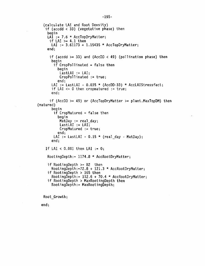
-195-

{calculate LAI and Root Density} if (accdd < 33) {vegetative phase} then begin LAI := 7.6 * AccTopDryMatter; if LAI>= 4.1 then

LAI := 3.61173 + 1.15435 * AccTopOryMatter; end;

if (accdd >= 33) and (AccOD < 49) {pollination phase} then begin if CropPollinated = false then

begin LastLAI := LAI; CropPollinated := true;

end; LAI := LastLAI - 0.035 * (AccDD-33) * AccLAIStressfact; if LAI<= 0 then cropmatured := true; end;

if (AccDD >= 49) or (AccTopDryMatter >= plant.MaxTopDM) then {matured}

begin if CropMatured = false then

begin MatDay := real day; LastLAI := LAI; CropMatured := true;

end; LAI := LastLAI - 0.15 * (real_day - MatDay);

end;

If LAI< 0.001 then LAI := O;

RootingDepth:= 1174.8 * AccRootDryMatter;

if RootingDepth >= 82 then RootingDepth:=72.8 + 121.3 * AccRootOryMatter;

if RootingDepth > 165 then RootingDepth:= 112.6 + 70.4 * AccRootDryMatter;

if RootingDepth > MaxRootingDepth then RootingDepth:= MaxRootingDepth;

Root_Growth;

end;

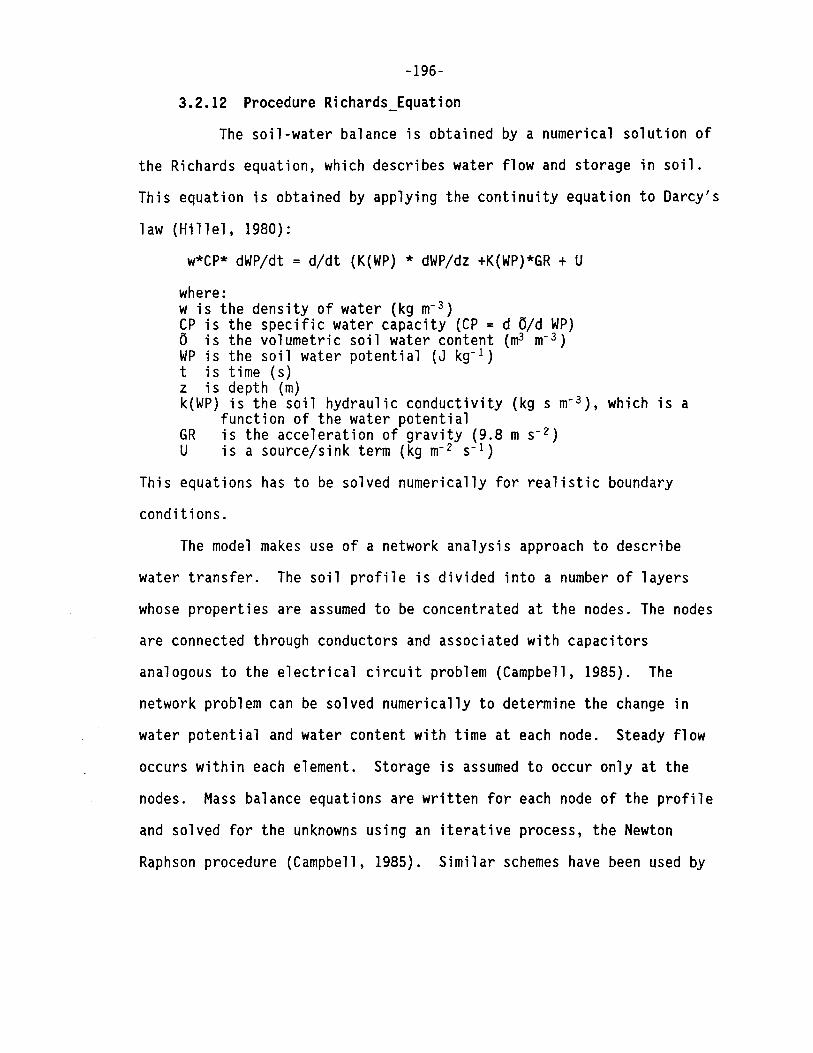
-196-

3.2.12 Procedure Richards_Equation

The soil-water balance is obtained by a numerical solution of

the Richards equation, which describes water flow and storage in soil.

This equation is obtained by applying the continuity equation to Darcy's

law (Hillel, 1980):

w*CP* dWP/dt = d/dt (K(WP) * dWP/dz +K(WP)*GR + U

where: w is the density of water (kg m- 3) CP is the specific water capacity (CP = d 0/d WP) 0 is the volumetric soil water content (m3 m-3) WP is the soil water potential (J kg- 1) t is time (s) z is depth (m) k(WP) is the soil hydraulic conductivity (kg s m- 3), which is a

function of the water potential GR is the acceleration of gravity (9.8 m s- 2) U is a source/sink term (kg m-2 s-1)

This equations has to be solved numerically for realistic boundary

conditions.

The model makes use of a network analysis approach to describe

water transfer. The soil profile is divided into a number of layers

whose properties are assumed to be concentrated at the nodes. The nodes

are connected through conductors and associated with capacitors

analogous to the electrical circuit problem (Campbell, 1985). The

network problem can be solved numerically to determine the change in

water potential and water content with time at each node. Steady flow

occurs within each element. Storage is assumed to occur only at the

nodes. Mass balance equations are written for each node of the profile

and solved for the unknowns using an iterative process, the Newton

Raphson procedure (Campbell, 1985). Similar schemes have been used by

-197-

Stoeckle (1985), Weaver (1984) and Bristow (1983) to describe different

aspects of the soil-plant-atmosphere continuum.

The procedure Richards Flow simulates infiltration,

redistribution, and soil evaporation. Input requirements for the

procedure Richards Flow include soil physical parameters such as bulk

density, partical density, saturated hydraulic conductivity, air entry

potential, and soil b-value. If these parameters have not been

measured, they can be estimated from soil textural data (Campbell,

1985). The procedure Richards_Flow is divided into separate procedures.

These procedures will be discussed in the sequence of their being called

in the procedure Richards_Flow.

The procedure Hydraulic_Conductivities calculates unsaturated

hydraulic conductivities for each layer using the soil water potentials

of the most recent time step (or the initial soil water potentials at

the beginning of a simulation). The unsaturated hydraulic conductivity

(K) for each soil profile layer is calculated according to Campbell

(1974):

(1) K(I) = soil.HydCond(I) * (soil.AirEntryPot(I) /

sim.WP(I))AN(I)

where: soil.HydCond is the saturated hydraulic conductivity (kg s m-3) soil.AirEntryPot is the air entry potential (J kg- 1 ) sim.WP is the soil water potential (J kg-1) N = 2+3/soil.BValue, where soil.BValue is the slope of the water release curve, when plotted

on log/ log scale.

The procedure Soil_Evaporation determines actual soil evaporation.

First, the relative humidity (HA) of the soil surface layer is

calculated from the soil water potential:

-198-

(2) HA= exp(MW*sim.WP[2]/(R*(sim.Soi1Temp[2]+273)))

where: MW is the molecular weight of water (0.018 kg mole- 1 ) sim.WP[2] is the soil surface node water potential (J kg- 1 ) R is the gas constant (8.3143 J mole- 1 K-l) sim.Soiltemp is the soil temperature (°C) (Addition of 273 converts °C into Kelvin).

The actual evaporative flux (EV) of water from the surface layer is then

calculated as:

(3) sim.EV[l] = sim.PotEva * (HA-clim.RelHumid[day])/(1-clim.RelHumid[-

day]))

where: sim.PotEva is the potential soil evaporation rate (kg m- 2 s- 1 )

clim.RelHumid is the relative humidity of the air HA is the relative humidity of the soil surface node

Evaporation during second and third stage drying is controlled by the

humidity of the evaporative surface and the liquid flux to the soil

surface from deeper soil layers. The derivative of the evaporative flux

is calculated for use later:

(4) DEV[l]=sim.PotEva*MW*HA/(R*(sim.SoilTemp[2]+273)*(1 -

clim.RelHumid[DAY]))

In the procedure Jacobian the components of the Jacobian matrix and

mass balance terms are calculated. The water flux (WFlux) (positive

downward) in element I is:

(5) sim.WFlux(I) = -(K[I+l]*sim.WP[I+l] - K[I]*sim.WP[I])

/((soil.NodeDepth[I+l]-soil.NodeDepth[I])*(l-N))

where: soil.NodeDepth is the depth of the soil node (m)

Combining this equation with the mass balance equation for a layer:

(6) FGauss[l]=WFlux[l-l]-WFlux[I]+U(l-1)-U(I)+ Volume[I]*(WN[I]-W[I]) *

time_step

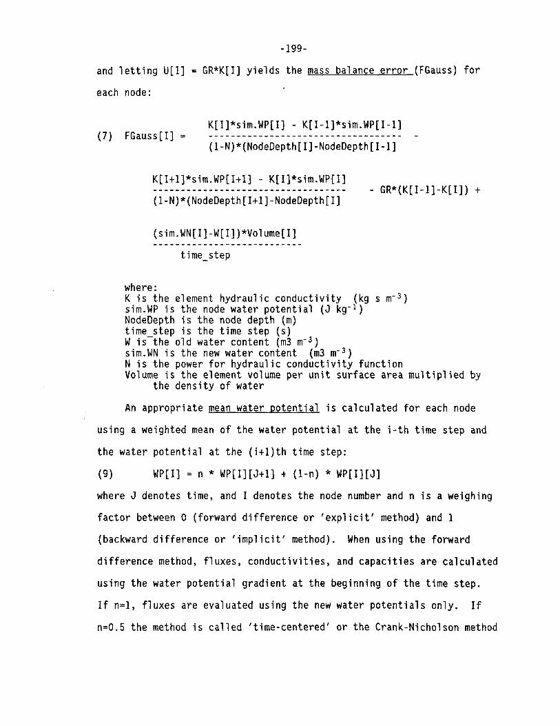
-199-

and letting U[I] = GR*K[I] yields the mass balance error (FGauss) for

each node:

(7) FGauss[I] = K[I]*sim.WP[I] - K[I-l]*sim.WP[I-1]

(l-N)*(NodeDepth[I]-NodeDepth[I-1]

K[I+l]*sim.WP[I+l] - K[I]*sim.WP[I]

(1-N)*(NodeDepth[I+l]-NodeDepth[I]

(sim.WN[I]-W[I])*Volume[I]

time_step

where:

- GR*{K[I-1]-K[I]) +

K is the element hydraulic conductivity (kg s m- 3 ) sim.WP is the node water potential (J kg- 1 ) NodeDepth is the node depth (m) time step is the time step (s) Wis-the old water content (m3 m- 3 )

sim.WN is the new water content (m3 m- 3 ) N is the power for hydraulic conductivity function Volume is the element volume per unit surface area multiplied by

the density of water

An appropriate mean water potential is calculated for each node

using a weighted mean of the water potential at the i-th time step and

the water potential at the (i+l)th time step:

(9) WP[I] = n * WP[I][J+l] + (1-n) * WP[I][J]

where J denotes time, and I denotes the node number and n is a weighing

factor between O (forward difference or 'explicit' method) and 1

(backward difference or 'implicit' method). When using the forward

difference method, fluxes, conductivities, and capacities are calculated

using the water potential gradient at the beginning of the time step.

If n=l, fluxes are evaluated using the new water potentials only. If

n=0.5 the method is called 'time-centered' or the Crank-Nicholson method

-200-

and the arithmetic average of the water potential at the beginning and

end of the time step is used to calculate fluxes of water. The choice

of n depends on the time constant of the system and strongly affects the

numerical stability and accuracy of the solution. When n=O the solution

can be unstable if the time steps chosen are too large or the fluxes of

water entering the profile are great. For water flow problems, n=l

almost always gives the best results and will be used hereafter.

Other sources/sinks not represented in Eq. 6, such as root

extraction, gravitational flux, precipitation, or irrigation, are added

explicetly to the mass balance term in equation 7 and such become part

of the solution.

Eq. 7 can be written for each node in the simulated soil profile

resulting in Lastlayer equations in Lastlayer+2 unknowns. Boundary

conditions are used to reduce the number of unknowns by two so that the

system of equations can be solved simultaneously. The three basic

choices for boundary conditions are measured values, assumed constant

flux and assumed constant potential. For the profile's upper boundary,

the soil water potential can be set to the air entry potential during

infiltration in order to simulate saturation, or to a specified flux

density in the case where the water input is less than the infiltration

rate. At the bottom of the profile, the potential is usually set to a

known value, for example zero for a water table. The potential could be

set at some value that can be considered constant for the duration of

the run. Or there could be some depth at which no water flux is assumed

to occur.

-201-

Writing Eq. 7 for each node and expressing the set of simultaneous

equations as a tridiagonal matrix results in the Jacobian matric:

BGauss(l) CGauss(l) AGauss(2) 8Gauss(2) 0 AGauss(3) 0 0

where:

0 CGauss(2) BGauss(3) AGauss(4)

0 0 CGauss(3) 8Gauss(4)

DP(l) DP(2) DP(3) DP(4)

FGauss[I] is the mass balance error for node I,

(10) CGauss[I] = d FGauss[I]/d sim.WP[I+l] = -K[I+l]/(NodeDepth[I+l)-NodeDepth[I])

FGauss(l) FGauss(2) FGauss(3) FGauss(4)

(11) BGauss[I] = d FGauss[I]/d sim.WP[I] = K[I]/(NodeDepth[I]NodeDepth[I-l])+K[I]/(NodeDepth[I+l] -NodeDepth[I])+CPcI]) - GR*N[I]*K[I]/sim.WP[I] + sim.DEV[I-1]-sim.DEV[I]

(12) AGauss[I] = d FGauss[I]/d WP[I-1] = -K[I-l]/(NodeDepth[I]NodeDepth[I-1]) + GR*N[I]*K[I-l]/sim.WP[I-1]

DP[I] is the change in water potential over one iteration·

The node soil water capacity term (CP) is calculated as:

(8) CP[I] =-Volume[!]* sim.WN[I]/(soil.BValue[I]*

sim.WP[I]*time step)

where: Volume is the volume per unit area of the soil time_step is the time step (sec) sim.WN is the water content (m3 m-3) soil.BValue is the soil b-value (slope of the water release curve)

The coefficient matrix consists of the partial derivatives

(AGauss,BGauss, and CGauss) of each FGauss[I] with respect to each node

water potential influencing it.

After each iteration, the total mass balance error (SE) for the

whole soil profile is evaluated by summing the mass balance errors from

all the nodes:

(13) SE=SE+ABS(FGauss[I])

-202-

Convergence is determined by checking whether the FGauss[I]'s are

sufficiently close to zero. When the total mass balance error is less

than the allowable mass balance error the procedure is completed.

In the procedure Thomas_Algorithm the set of equations is solved by

Gauss elimination and a new set of soil water potential changes (DP[I])

is found and once again substituted into the Jacobian matrix. The soil

water potential changes for each layer (DP[I]) are calculated and the

old water potential is updated for each node:

(14) DP[I] = FGauss[I] - CGauss * DP[I+l]

(15) sim.WP[I] = sim.WP[I] - DP[I]

When the DP[I]'s for all the nodes in the profile become zero,.the

correct values for the soil water potentials have been found.

Convergence is determined by checking whether the FGauss[I]'s are

sufficiently close to zero. When the total mass balance error (IM) is

less than the allowable mass balance error the procedure is completed.

These are also the values at which mass balance is assured. The water

potential is not allowed to exceed the air entry value and is set to the

air entry value if the calculated new water potential exceeds the air

entry potential.

In the procedure New_Water_Contents the new water contents (WN) for

each layer are calculated from the updated water potentials:

(16) sim.WN[I] = WS[I] * (soil.AirEntryPot[I] / sim.WP[I])AB1[IJ

where: WS is the saturated water content (m3 m- 3 ) soil.AirEntryPot is the air entry potential (J kg- 1) sim.WP is the water potential (J kg- 1) Bl is the inverse of the soil 8-value.

-203-

0nce the solution satisfies mass balance criteria, the procedure

Calculate_Fluxes calculates the changes in amount of water for each

layer and the whole profile. Fluxes between layers are also calculated

and the new water contents for the next time step are updated.

At each time step the water content change for each node in the

profile is calculated:

(20) Node_WC_Chg[I] = Volume[I]*(sim.WN[I]-W[I])

where: Volume is the volume of soil per unit area soil surface (m) sim.WN is the water content of the next time step (m3 m-3) Wis the old water content (m3 m-3)

The changes for each node are summed up to get the change in amount of

water for the whole profile, and the rate of change is calculated:

(21)

(22)

Profile WC Chg:= Profile WC Chg+ Node WC Chg[I] - - - - - -Profile_WC_Chg_Rate:= Profile_WC_Chg / time_step

where: Profile WC Chg is the change in amount of water in the profile over

one time step Profile_WC_Chg_Rate is the rate of change of water content for the

profile Time_step is the time step (sec)

The new water contents for the next time step are updated:

(23) sim.WN[I] = W[I]

and the drainage from the lower boundary of the soil profile

is calculated. Assuming no matric potential induced flux at the bottom

of the soil profile the drainage rate is:

(24) Drain_Rate =GR* K[Nlayer]

where: GR is the acceleration of gravity (9.8 m s-2) K[Nlayer] is the hydraulic conductivity of the bottom layer (kg s

m-3)

-204-

List of References

Bristow, K.L. 1983. Simulation of heat and moisture transfer through a surface residue-soil system. Ph.D. thesis. Washington State University, Pullman.

Campbell, G.S. 1985. Soil Physics with Basic. Transport Models for Soil-Plant Systems. Elsevier, New York. 149 pp.

Campbell, G.S. 1974. A simple method for determining unsaturated hydraulic conductivity from moisture retention data. Soil Sci. 117:311-314.

Hillel, D. 1980. Fundamentals of Soil Physics. Academic Press, New York.

Stoeckle, C.O. 1985. Simulation of the effect of water and nitrogen stress on growth and yield of spring wheat. Ph.D. thesis. Washington State University, Pullman.

Weaver, H.L. 1984. A mechanistic model of evapotranspiration from Saltcedar. Ph.D. thesis. Washington State University, Pullman.

Procedure const

GR


Richards_Equation;

IM

var SE K

AGauss, CGauss, BGauss FGauss I

= 9.8; = lE-6;

real; depth;

{accelleration of gravity, m s-2} {allowable mass balance error, kg m-2

s-1}

{mass balance error, kg m-2 s-1} {unsaturated hydr. conductivity, kg s

m-3}

depth; {partials in Jacobian matrix} depth; {mass balance term, kg m-2 s-1}

: integer; {counter variable} {---------------------------------------------------------}

Procedure Campbell Hydraulic Conductivities; var I : integer; -

begin For I := 2 to soil.Lastlayer+l do K[I] := soil.HydCond[I].value *

POW((soil.AirEntryPot[I].value/sim.WP[I]),N[I]); end; {Hydraulic_Conductivities}

{---------------------------------------------------------}

-205-

Procedure Soil Evaporation; canst -

MW= 0.018; R = 8.31;

{molecular weight of water} {gasconstant}

var HA: real; {soil surface relative humidity}

begin HA:= EXP( MW* sim.WP[2] / (R*(sim.Soi1Temp[2]+273))); sim.EV[l] := sim.PotEva*(HA-clim.RelHumid[real_day].value)/

(1-clim.RelHumid[real_day].value); DEV[l] := sim.PotEva*MW*HA/ (R*(sim.Soi1Temp[2]+273) *

(1-clim.RelHumid[real_day].value)); end; {Soil_Evaporation}

{---------------------------------------------------------} Procedure Jacobian;

var CP : depth; {soil node water capacity} I : integer;

begin K[l]:=0; SE := O; For l:=2 to soil.Lastlayer do

begin CP[I] := -Volume[I]*sim.WN[I]/(soil.BValue[I].value

*sim.WP[l]*time step); AGauss[l]:=-K[l-1]/(soil.NodeDepth[i].value -

soil.NodeDepth[i-1].value)+GR *N[I]*K[I-1]/sim.WP[I-1];

CGauss[l]:=-K[l+l]/{soil.NodeDepth[i+l].value -soil.NodeDepth[i].value);

BGauss[I]:=K[I]/(soil.NodeDepth[i].value -soil.NodeDepth[i-1].value)+K[I]/ (soil.NodeDepth[i+l].value -soil.NodeDepth[i].value) + CP[I] -GR*N[I]*K[I]/sim.WP[I]+DEV[l-l]+DEV[I];

FGauss[l]:=((sim.WP[l]*K[I]-sim.WP[I-l]*K[I-1])/ (soil.NodeDepth[i].value -soil.NodeDepth[i-1].value)-(sim.WP[I+l] * K[I+l] - sim.WP[I] * K[I])/ (soil.NodeDepth[i+l].value -soil.NodeDepth[i].value))/Nl[I]+Volume[I] *(sim.WN[I]-W[I])/time_step - GR*(K[l-l]-K[I])+sim.EV[l-1] -sim.EV[I]+sim.WUptake[I]-Winput[I];

SE := SE+ABS(FGauss[I]);

end; end; {Jacobian}

{---------------------------------------------------------}

-206-

Procedure Thomas Algorithm; var DP : depth; {change in water potential}

I : integer; begin {Gauss elimination}

for I:=2 to soil.Lastlayer-1 do begin

CGauss[I] FGauss[I] BGauss[I+l] FGauss[I+l]

end;

:= CGauss[I]/BGauss[I]; := FGauss[I]/BGauss[I]; := BGauss[I+l]-AGauss[I+l]*CGauss[I]; := FGauss[I+l]-AGauss[I+l]*FGauss[I];

DP[soil.Lastlayer]:=FGauss[soil.LastLayer]/BGauss[soil.Lastlayer];

sim.WP[soil.Lastlayer]:=sim.WP[soil.Lastlayer]-DP[soil.Lastlayer]; if sim.WP[soil .Lastlayer]>soil.AirEntryPot[soil.Lastlayer].value

then sim.WP[soil.Lastlayer] := soil.AirEntryPot[soil.Lastlayer].value;

{back substitution} for I:=soil.Lastlayer-1 downto 2 do

begin DP[I]:=FGauss[I]-CGauss[I]*DP[I+l]; sim.WP[I]:=sim.WP[I]-DP[I]; if sim.WP[I] > soil.AirEntryPot[I].value

then sim.WP[I] := soil.AirEntryPot[I].value; end;

end; {Thomas Algorithm}

{---------------------------------------------------------} Procedure New Water Contents; var I : Tnteger;

begin for I:=2 to soil.Lastlayer do

sim.WN[I]:=WS[I]*POW(soil.AirEntryPot[I].value/sim.WP[I], 1/soil.BValue[I].value);

sim.WP[soil.Lastlayer+l] := sim.WP[soil.Lastlayer]; sim.WN[soil.Lastlayer+l] := sim.WN[soil.Lastlayer];

end; {New_Water_Contents}

{---------------------------------------------------------} Procedure Calculate_Fluxes;

var Profile WC Chg Node WC-Chg I : Tnteger;

begin {calculate changes

real; depth;

in water contents}

-207-

Profile WC Chg:=0; For I:=2 to soil.Lastlayer do

begin Node WC Chg[!]:= Volume[!]* (sim.WN[I]-W[I]) ; ProfTle=WC_Chg:= Profile_WC_Chg + Node_WC_Chg[I]; WC Change:= Profile WC Chg/ time step; sim.WFlux[I]:=((K[IJ*sTm.WP[I] - K[I+l]*sim.WP[I+l])/

end;

( Nl[I] * (soil.NodeOepth[I+l].value -soil.NodeOepth[I].value)) +GR* K[I]);

{reset water contents for next time step} For I:= 2 to soil.Lastlayer do

W[I]:=sim.WN[I];

Drain_Rate:= GR* K[soil.Lastlayer];

end; {Calculate_Fluxes}

begin {Richards Equation} Repeat

Campbell Hydraulic Conductivities; Soil Evaporation; -Jacobian; Thomas_Algorithm; New Water Contents;

Until-(SE <-IM); Calculate Fluxes;

end; {Richards_Equation}

List of Variables

Global Variables:

sim.WP soil water potential (J kg-1)

soil water content (m3 m-3) w sim.WN

soil.HydCond

sim.EV

sim.WUptake

Wlnput

new soil water content (m3 m- 3 )

Saturated soil hydraulic conductivity (kg s m-3)

soil evaporative flux (kg m-2 s-1)

root water uptake (kg m-2 s-1)

Irrigation and/or precipitation (kg m-2 s-1)

sim.SoilTemp

sim.PotEva

Volume

DEV

Local Variables:

K

SE

I

HA

DP

CP

AGauss

BGauss

CGauss

FGauss

Local Constants:

MW

R

GR

IM

-208-

Soil temperature (°C)

potential soil evaporation (kg m-2 s- 1 )

Volume of soil layer per unit area multiplied by the

density of water

derivative of evaporative flux

soil hydraulic conductivity (kg s m-3)

mass balance error (kg m-2 s-1)

counter variable

relative humidity of the surface node

change in water potential over a time step

node water capacity (d 0/d WP)

partial derivative of FGauss with respect to WP[I-1]

(sub diagonal element in tridiagonal matrix)

partial derivative of FGauss with respect to WP[I]

(diagonal element in tridiagonal matrix)

partial derivative of FGauss with respect to WP[I+l]

(super diagonal element in tridiagonal matrix)

node mass balance error (kg m-2 s- 1)

Molecular weight of water (0.018 kg mole- 1)

gas constant (8.3143 J mole-1 K-1)

acceleration of gravity (9.8 m s-2)

maximum allowable mass balance error (lE-06 kg m- 2

s- 1 )

-209-

3.2.13 Procedure Tipping_Bucket_Flow

This procedure uses the soil water flow approach as contained in

the CERES Maize model (Jones and Kiniry, 1986). The code as contained

in CERES Maize was translated into Pascal with concommitant changes in

the programming but without altering the general computational method.

As the name of this procedure suggests the soil is conceptualized

as consisting of a series of tipping buckets each having a specified

capacity to hold water. Each 'bucket' corresponds to a soil layer the

dimensions and properties of which have to be specified in the soil

input data file. Basically, water is transferred from one layer to the

next downward in the soil profile if the amount entering the layer

exceeds the layer's water holding capacity. The capacity of each soil

layer to hold water is calculated as the difference between the

saturation water content (WS) and the current volumetric water content.

Input requirements for this procedure include values for bulk density

and particle density to calculate saturation water content, field

capacity or 'Drained Upper Limit' (DUL) and wilting point or 'Lower

Limit' volumetric water contents (LL). The values of DUL and LL can be

estimated from soil textural data and organic carbon content using

empirical equations contained in CERES Maize (Ritchie et al., 1986).

Ideally, values for DUL and LL should be obtained from field

measurements as described by ....... ( ). Empirical equations to

estimate these parameters can be found in Appendix A.

-210-

The Profile Drainage Coefficient (Profile_SWCON) used in

calculating the amounts of water drained from a layer is estimated in

the procedure Estimate Parameters by calculating a Drainage coefficient

for each layer (SWCON) and using the smallest one as the value for the

whole profile.

(1) SWCON[I]:=(PO[I]-soil .DUL[I])/PO[I]

where: PO is the soil total porosity soil.DUL is the field capacity water content

The procedure Clear sets the variables Drain Rate and Flux[!] to

zero before each time step calculation.

In the procedure Water_Application the flux into the first soil

layer (Flux[2]) is set equal to precipitation. The daily amount of

water is distributed evenly over the whole day by dividing the amount of

water added by the number of time steps in a day:

(2) Flux[2]:=(clim.Precip[real_day].value)/ num_of_time_steps;

where: clim.Precip is measured daily precipitation (mm/day) num_of_time_steps is the number of time steps per day

If the resulting flux is greater than zero the procedure Infiltration is

called. In this procedure the amount of water the layer can hold is

calculated as the amount of water between saturation water content and

the current water content:

(3) Hold:=(WS[I]-sim.WN[I]) * Volume[!]

where: Volume is the volume of the soil layer per unit surface area (m) WS is the saturation water content (m3 m- 3) sim.WN is the soil layer water content (m3 m-3)

If the flux into the layer is greater than Hold the procedure

Saturated Flow calculates the water draining to the next layer (Drain),

-211-

the new water content of the node (sim.WN) and updates the flux to be

passed on to the next downstream layer.

(4) Drain:=Profile SWCON*(WS[I]-DUL[I])*Volume[I]

(5) sim.WN[I]:=WS[I]-Drain/Volume[I];

(6) Flux[I]:=Flux[I]-Hold+Drain;

If the flux does not exceed Hold the old water content of the layer is

updated:

(7) sim.WN[I]:=sim.WN[I]+Flux[I]/Volume[I];

If this new water content exceeds the Drained upper limit water content

(field capacity) the procedure Unsaturated_Flow is called to calculate

fluxes, new water contents and update the flux passed to the downstream

layer similiar to procedure Saturated_Flow.

(8) Drain:=Profile SWCON*(sim.WN[I]-DUL[I])* Volume[!]

(9) sim.WN[I]:=sim.WN[I]-Drain/Volume[I]

(10) Flux[I]:=Drain

The amount of water returned in Flux[I] from the procedure Infiltration

is passed on to the next soil layer repeating the process until the

bottom layer of the soil profile has been reached. If there is a

residual flux left after satisfying the water holding capacity of all

layers in the soil profile the remaining flux is declared drainage from

the bottom of the profile (Drain Rate).

Soil evaporation is included in the Tipping Bucket water flow

procedure as simple first-stage evaporation, which is allowed to proceed

until the soil water content reaches 50 % of its value at permanent

wilting point. Soil evaporation occurs only from the surface soil node.

No upward water flow is simulated. First, the amount of water available

-212-

for soil evaporation is calculated as half the amount of water between

the permanent wilting point (LL) and the current soil water content

(WN):

AvailableWater := (Volume[!]* (sim.WN[I]-soil.DLL[I].value/2))

Actual soil evaporation is allowed to proceed at potential rates and is

limited only by the amount of water present in the uppermost soil layer.

Under non-limiting conditions:

sim.Ev[l] = sim.PotEva

When the amount of water present becomes limiting, soil evaporation is

limited to that amount:

sim.Ev[l]:= AvailableWater / time_step

Then the water contents are updated:

sim.WN[I]:=sim.WN[I] - ((sim.EV[l]*time_step)/volume[I])

At the end of the time step the procedure Calculate_Fluxes

calculates the changes in water contents for each node and the overall

profile, as well as fluxes of water between the layers. The old water

contents are updated:

(11) W[I]:=sim.WN[I];

At each time step the water content change for each node in the

profile is calculated:

(12) Node_WC_Chg[I] = Volume[I]*(sim.WN[I]-W[I])

where: Volume is the volume of soil per unit area soil surface (m) sim.WN is the water content of the next time step (m3 m-3) Wis the old water content (m3 m-3)

The changes for each node are summed up to get the change in amount of

water for the whole profile, and the rate of change is calculated:

(13) Profile WC Chg:= Profile WC Chg+ Node WC Chg[I] - - - - - -

-213-

(14) Profile_WC_Chg_Rate:= Profile_WC_Chg / time_step

where: Profile WC Chg is the change in amount of water in the profile over

one tTme step Profile WC Chg Rate is the rate of change of water content for the

profile -Time_step is the time step (sec)

List of References

Jones, C.A. and J.R. Kiniry. (eds). 1986. CERES-Maize. A simulation model of maize growth and developement. Texas A&M University Press, College Station. 194 pp.

Jones, C.A., J.T Ritchie, J.R. Kining and D.C. Godwin. 1986. Subroutine Structure. In: CERES-Maize. A Simulation Model of Maize Growth and Development. C.A. Jones and J.R. Kiniry (Eds). Texas A&M University Press, College Station. 194 pp.

Ritchie, J.T., J.R. Kining, C.A. Jones and P.T. Dyke. 1986. Model Inputs. In: CERES-Maize. A Simulation Model of Maize Growth and Development. C.A. Jones and J.R. Kiniry (Eds). Texas A&M University Press, College Station. 194 pp.


Procedure Tipping_Bucket_Flow;

{"tipping bucket" water balance approach as used in CERES MAIZE, Ritchie et al., 1986.}

var J I Hold

Flux SWCON Profile SWCON Drain PO

integer; integer; real;

depth; depth; real; real; depth;

Procedure Estimate_Parameters; var I : integer;

{counter variable} {counter variable} {amount of water soil can hold above

present level,cm} {flux of water into next layer, cm} {layer drainage coefficient} {profile drainage coefficient} {drainage= flux, cm} {soil porosity, cm3/cm3}

-214-

begin Profile SWCON:=1.00; For I:=-2 to soil.Lastlayer do begin PO[I]:= WS[I]; SWCON[I]:={PO[I]-soil.DUL[I].value)/PO[I]; If SWCON[I] < Profile SWCON

then Profile SWCON:=SWCON[I]; end; {for layers do .. }

end; {Estimate Parameters}

{------------------------------------------------} Procedure Null Setting;

var I : integer; begin for l:=2 to soil.Lastlayer do

Flux[!] := 0.0; Drain Rate := 0.0;

end; (Null_Setting}

{------------------------------------------------} Procedure Soil_Evaporation; var

I AdditionalDemand AvailableWater

integer; real; real;

begin AvailableWater:=0; AdditionalDemand:=0;

For I:= 2 to 2 do begin

AvailableWater := (Volume[I] * (sim.WN[I] -soil.DLL[I].value/2}};

if AvailableWAter <= 0 then AvailableWater := O; sim.Ev[l]:= sim.PotEva; if (sim.PotEva*time step)> AvailableWater then

begin -Additiona1Demand:= sim.PotEva*time step -

AvailableWater;sim.Ev[l]:= AvailableWater / time step;

end; -

sim.WN[l]:=sim.WN[I] - ((sim.EV[l]*time_step)/volume[I]); end;

end; {Soil_Evaporation}

{------------------------------------------------} procedure Infiltration;

-215-

procedure Saturated_Flow; begin

Drain:=Profile SWCON*(WS[I]-soil.DUL[I].value)* Volume[!]; sim.WN[I]:=WS[T]-Drain/ Volume[!] -

((sim.WUptake[I]*time_step)/volume[I]);; Flux[I]:=Flux[I]-Hold+Drain;

end; {Saturated_Flow}

procedure UnSaturated_Flow; begin

Drain:=Profile SWCON*(sim.WN[I]-soil.DUL[I].value)*volume[I]; sim.WN[I]:=sim~WN[l]-Drain/volume[I]; Flux[I]:=Drain;

end; {UnSaturatedFlow}

Begin {Infiltration} Hold:=(WS[I]-W[I])*volume[I]; IF Flux[I] > Hold then

Saturated Flow else -begin

sim.WN[I]:=W[I]+Flux[l]/volume[I] -((sim.WUptake[I]*time_step)/volume[I]);;

if (sim.WN[I] > soil.OUL[I].value+0.003) then Unsaturated Flow

else -Flux[I]:=0;

end; end; {Infiltration} {------------------------------------------------} Procedure Calculate_Fluxes;

var Profile WC Chg Node WC-Chg I : Tnteger;

begin

real; depth;

{calculate changes in water contents} Profile WC Chg:=0; For I:=2 to soil.Lastlayer do

begin Node_WC_Chg[I]:= Volume[!]* (sim.WN[I]-W[I]); Profile WC Chg:= Profile WC Chg+ Node WC Chg[I]; WC_Change:; (Profile_WC_Chg-- Orain_Rate)-/ time_step

end;

{reset water contents for next time step} For I:= 2 to soil.Lastlayer do

W[I]:=sim.WN[I];

-216-

end; {Calculate Fluxes} {------------------------------------------------}

Begin {tipping bucket} Estimate Parameters; Null Setting; Flux[2]:= Winput[2] * time step; for I:= 2 to soil .LastLayer do

begin if Flux[!]> 0 then Infiltration else sim.WN[I]:=W[I]+Flux[I]/volume[I] -

((sim.WUptake[I]*time step)/volume[I]);;

if I< soil.LastLayer then Flux[I+l]:=Flux[I] else Drain Rate:=Flux[I] / time step; {in mm}

end; {For.~ to soil.LastLayer} -Soil Evaporation; Calculate Fluxes;

end; {tipping_bucket}

Global Variables:

w sim.WN

Drain Rate

Volume

ws soil .bulk_density

soil.part_density

soil.DUL

soil.LL

Local Variables:

J

SWCON

List of Variables

soil water content (m3/m3)

new soil water content (m3/m3)

drainage from bottom of profile (mm)

volume per unit surface area

saturation water content

soil bulk density

soil particle density

drained upper limit (field capacity)

lower limit (wilting point)

counter variable

layer drainage coefficient

HOLD

present level (mm) Flux

Profile SWCON

Drain

PO

Profile_WC_Chg

Node_WC_Chg

-217-

amount of water soil can hold above

flux of water into next layer (mm)

profile drainage coefficient

drainage= flux (mm)

soil porosity (cm3/cm3)

change in water content in the soil

profile over one time step

change in water content of one layer over

one time step

3.2.14 Procedure Water_Budget

The procedure Water Budget adds up rates of several variables

related to the water budget of the soil-plant system during the day and

converts rates expressed in kg m- 2 s- 1 at the time step level into units

of mm/day. These variables are saved to the output file *.SUM if the

option 'Out' is chosen in the simulator menu before starting a

simulation.

The procedure Water_Budget is called automatically regardless of

the model implemented by the user.


Procedure Water_Budget;

var I : integer;

begin ProfileWater:=0; Profil eAva il : =0;

end;

-218-

{sums up and converts to mm/day) SumPotTrans:=SumPotTrans + sim.PotTrans * time step; SumPotEV:=SumPotEV + sim.PotEva * time step; -SumEV:=SumEv + sim.EV[l] * time step; -SumWCChange:=SumWCChange + WC_Change * time_step; SumDrain:=SumDrain + Drain Rate* time step; SumActTrans:=SumActTrans +-ActTrans * time step; SumWI:=SumWI+Winput[2] * time step; -sim.PotET:=sim.PotET + sim.ETP * time step; NetHeatFlux:=NetHeatFlux + sim.HeatFlux/num of time steps; - - -For I:= 2 to soil.Lastlayer do

begin LayerWater[I]:= Volume[!]* sim.WN[I]; LayerAvail[I]:= Volume[!]* (sim.WN[I] -

soil.LL[I].value); if LayerAvail[IJ < 0 then LayerAvail[I]:= O;

ProfileWater := ProfileWater + LayerWater[I]; ProfileAvail := ProfileAvail + LayerAvail[I];

end;

List of Variables

Global Variables:

SumPotTrans

SumPotEV

SumEV

SumWCChange

SumDrain

SumActTrans

SumWI

sim.PotET

NetHeatFlux

sim.HeatFlux

potential transpiration (mm/day)

potential soil evaporation (mm/day)

actual soil evaporation (mm/day)

soil profile water content change (mm/day)

drainage from bottom of soil profile (mm/day)

actual transpiration (mm/day)

total water input (irrigation plus

precipitation) (mm/day)

potential evapotranspiration (mm/day)

daily net heat flux accross soil surface

(positive downwards) (W m- 2)

soil heat flux accross soil surface (positive

downwards) (W m-2)

LayerWater

LayerAvail

Profi 1 eWater

ProfileAvail

Volume

soil . LL

sim.WN

-219-

amount of water contained in a layer (mm)

amount of plant available water in a layer (mm)

amount of water in profile (mm)

amount of plant available water in profile (mm)

Volume of soil per unit area (m)

wilting point soil water content (m3 /m- 3 )

current water content (m3 / m- 3 )

3.2.15 Procedure Water_Uptake

The amount of water flowing from soil to roots is directley

dependent on how much more negative the root water potential (RootWP} is

compared to the soil water potential (WP} (Gardner, 1960). Water flow

into roots has also been considered inversely dependent on the

resistance to water flow in the soil and in the root (Gardner and Ehlig,

1962). If we combine these two concepts with the assumption that there

is steady state water flow through the plant (i.e. there is no change in

the amount of water stored in the plant), then the following equation

can be written:

(1) sim.PotTrans = - (RootWP[I]-sim.WP[I]+soil.NodeDepth[I]*GR) /

Res[I]

where: sim.PotTrans is the water uptake by the plant {kg m-2 s-1) I is the soil layer and node number RootWP is the root water potential (J kg- 1 ) sim.WP[I] is the node soil water matric potential (J kg-1) soil.NodeDepth[I] is the depth of node I from the soil surface (m) GR is the acceleration of gravity (9.8 m s-2) Res[I] is the root and soil resistance of layer I (kg s m- 4 )

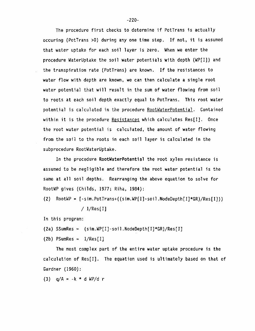
-220-

The procedure first checks to determine if PotTrans is actually

occuring (PotTrans >0) during any one time step. If not, it is assumed

that water uptake for each soil layer is zero. When we enter the

procedure WaterUptake the soil water potentials with depth (WP[I]) and

the transpiration rate (PotTrans) are known. If the resistances to

water flow with depth are known, we can then calculate a single root

water potential that will result in the sum of water flowing from soil

to roots at each soil depth exactly equal to PotTrans. This root water

potential is calculated in the procedure RootWaterPotential. Contained

within it is the procedure Resistances which calculates Res[I]. Once

the root water potential is calculated, the amount of water flowing

from the soil to the roots in each soil layer is calculated in the

subprocedure RootWaterUptake.

In the procedure RootWaterPotential the root xylem resistance is

assumed to be negligible and therefore the root water potential is the

same at all soil depths. Rearranging the above equation to solve for

RootWP gives (Childs, 1977; Riha, 1984):

(2) RootWP = [-sim.PotTrans+((sim.WP[I]-soil .NodeDepth[I]*GR)/Res[I]))

/ 1/Res[I]

In this program:

(2a) SSumRes = (sim.WP[I]-soil.NodeDepth[I]*GR)/Res[I]

(2b) PSumRes = 1/Res[I]

The most complex part of the entire water uptake procedure is the

calculation of Res[I]. The equation used is ultimately based on that of

Gardner (1960):

(3) q/A = -k * d WP/d r

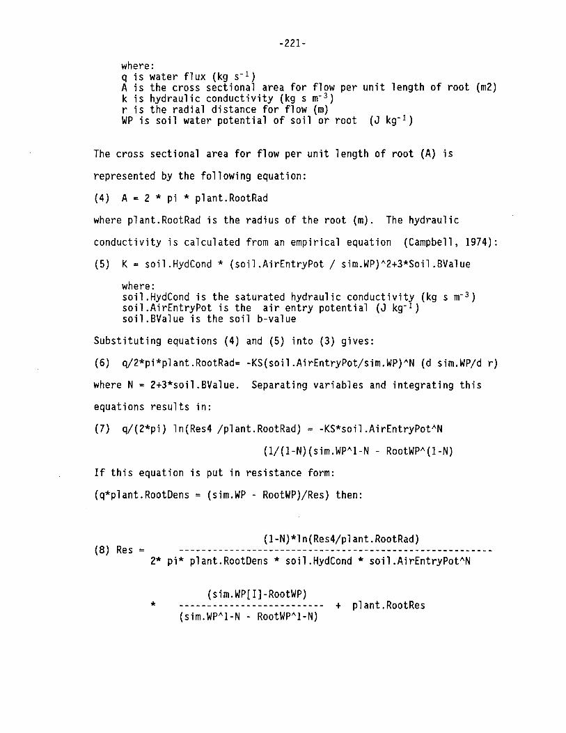
-221-

where: q is water flux (kg s- 1 ) A is the cross sectional area for flow per unit length of root (m2) k is hydraulic conductivity (kg s m- 3 ) r is the radial distance for flow (m) WP is soil water potential of soil or root (J kg- 1 )

The cross sectional area for flow per unit length of root (A) is

represented by the following equation:

(4) A= 2 *pi* plant.RootRad

where plant.RootRad is the radius of the root (m). The hydraulic

conductivity is calculated from an empirical equation (Campbell, 1974):

(5) K = soil.HydCond * (soil.AirEntryPot / sim.WP)A2+3*Soil .BValue

where: soil.HydCond is the saturated hydraulic conductivity (kg s m- 3 ) soil.AirEntryPot is the air entry potential (J kg- 1 ) soil.BValue is the soil b-value

Substituting equations (4) and (5) into (3) gives:

(6) q/2*pi*plant.RootRad= -KS(soil.AirEntryPot/sim.WP)AN (d sim.WP/d r)

where N = 2+3*soil.BValue. Separating variables and integrating this

equations results in:

(7) q/(2*pi) ln(Res4 /plant.RootRad) = -KS*soil.AirEntryPotAN

(1/(1-N)(sim.WPAl-N - RootWPA(l-N)

If this equation is put in resistance form:

(q*plant.RootDens = (sim.WP - RootWP)/Res) then:

(l-N)*ln(Res4/plant.RootRad) (8) Res=

2* pi* plant.RootDens * soil.HydCond * soil.AirEntryPotAN

(sim.WP[I]-RootWP) * -------------------------- + plant.RootRes

-222-

The distance from the center of the root to the point where sim.WP is

measured (RSoil) has been assumed to be (Gardner, 1960):

(9) Res4 =(pi* plant.RootDens)A -0.5

where plant.RootOens is the length of root per unit volume

of soil (m m-3).

Substituting eq. (9) into eq. (8) gives:

(1-N)*ln (1/RootRad*(pi*RootDens)AO.S)*(sim.WP[I]-RootWP) (10) Res=---------------------------------------------------------

-2*pi*RootDens*HydCond*AirEntryPotAN*(sim.WPA(l-NO)-RootWpA1-N)

The calculation of Res[I] is straightforward for the soil

resistance component of equation (10), when RootDens, RootRad, N,

sim.WP, KS, and PE are specified with depth. In procedure Resistances,

the calculation of RESI through RES4 solves the soil resistance

component of eq. (10) as a function of depth. Root resistance with

depth knowing the total root resistance is calculated as follows

(Campbell, 1986):

(11) RootRes[I] = RootRes/(RootDens[I]*LayThick[I])

where: LayThick[I] = length of the layer I (m), RootRes = Total plant root resistance (kg s m- 4 ).

Knowing the root water potential, RES[I] and sim.WP[I] the root

water uptake in each layer is easily calculated from the equation:

(12) sim.WUptake[I] = -(RootWP-sim.W~[I]+soil.NodeDepth[I]*GR)/Res[I]

-223-

List of References

Campbell, G.S. 1985. Soil Physics with BASIC: Transport models for soil-plant systems. NY Elsevier. 149 pp.

Campbell, G.S. 1974. A simple method for determining unsaturated hydraulic conductivity from moisture retention data. Soil Sci. 117:311-314.

Gardner, W. R. 1960. Dynamic aspects of water availability to plants. Soil Sci. 89:63-73.

Gardner, W. R. and C. F. Ehlig. 1962. Some observtions on the movement of water to the plant. Agron. J. 54:453-456.

Childs, S. W., J. R. Gilley and W. E. Splinter. 1977. A simplified model of corn growth under moisture stress. Trans. ASAE 20:858-865.

Riha, S. J. 1985. Estimating water fluxes in Douglas-fir plantations. Can. J. of For. Res. 5:701-707.


Procedure Water_Uptake(var RootWP:real);

const

var

GR AddP

i,j Res

Resl

Res2 Res3 Res4

PSumRes

SSumRes

= 9.8; =-200;

integer; depth;

depth;

depth; depth; depth;

real;

real;

{Acceleration of gravity,m s-2} {Constant to insure new root waterpotential is more negative than soil waterpotentials, J kg-1}

{counters} {Array ofroot and soil resistances as a function of depth} {Intermediate variable tocalculate Res}

{Array of soil resistances as a function of depth} {Summation of the root and soil conductances over all depths} {Summation of soil water potential divided by resistances over all depths}

-224-

procedure RootWaterPotential;

procedure Conductances; begin

Resl[j]:= -Nl[j]*ln(l/(RootRad*sqrt(pi*RootDens[j]))); Res2[j]:= Resl[j]/(2*pi*RootDens[j]*soil.conductivity[j].value

*POW(-soil.Air_entry_pot[j].value,N[j])); Res3[j]:=

Res2[j]*(sim.WP[j]-soil.node depth[j].value*GR-RootWP); Res4[j]:= -

Res3[j]/((POW((-sim.WP[j]+soil.node depth[j].value*GR), (-1-3/soil.B_value[j]~value))

-POW(-RootWP,(-1-3/soil.b value[j].value)))); Res[j] := Res4[j]+RootRes/(RootDens[j]*LayThick[j]); PSumRes:= 1/Res[j]+ PSumRes; SSumRes :=(sim.WP[j] - soil.node_depth[j].value*GR)/Res[j] +

SSumRes; end;

Begin RootWP:=RootWP+AddP; For I:=l to 3 do

Begin PSumRes:=O;SSumRes:=0;

For J:= FRoot to NRoot do Begin

If RootWP < (sim.WP[J]-soil.node_depth[J].value*GR) then

end; end;

Conductances else

Res[J]:=0;

RootWP := (-sim.PotTrans + SSumRes)/PSumRes; if RootWP < -1500 then RootWP:=-1500;

end; {RootWaterPotential)

procedure RootWaterUptake; var

i : integer; begin

ActTrans:= O; for i:= FRoot to NRoot do

if (Res[i] > 0) and (sim.WP[I] > -1500.0) then begin sim.WUptake[i] := -(RootWP-sim.WP[i]+

soil.node_depth[i].value*GR)/Res[i]; ActTrans:=sim.WUptake[i]+ActTrans;

end else

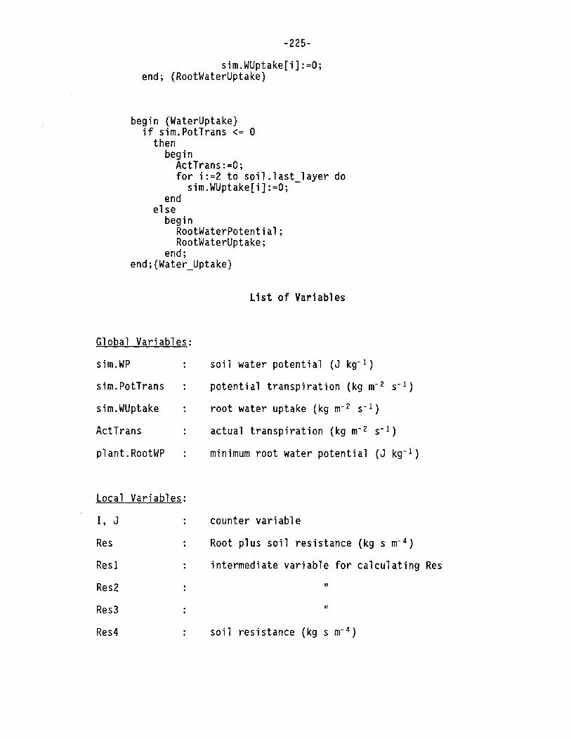
-225-

sim.WUptake[i]:=0; end; {RootWaterUptake}

begin {WaterUptake} if sim.PotTrans <= 0

then begin

ActTrans:=0; for i:=2 to soil.last layer do

sim.WUptake[i]:=0; -end

else begin

RootWaterPotential; RootWaterUptake;

end; end;{Water_Uptake}

List of Variables

Global Variables:

sim.WP

sim.PotTrans

sim.WUptake

ActTrans

plant.RootWP

soil water potential (J kg-1)


root water uptake (kg m-2 s-1)

actual transpiration (kg m-2 s-1)

minimum root water potential (J kg- 1)

Local Variables:

I, J

Res

Resl

Res2

Res3

Res4

counter variable

Root plus soil resistance (kg s m- 4 )

intermediate variable for calculating Res

II

II

soil resistance (kg s m- 4 )

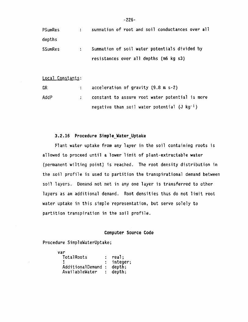
PSumRes

depths

SSumRes

-226-

summation of root and soil conductances over all

Summation of soil water potentials divided by

resistances over all depths (m6 kg s3}

Local Constants:

GR

AddP

acceleration of gravity (9.8 m s-2)

constant to assure root water potential is more

negative than soil water potential (J kg- 1 )

3.2.16 Procedure Simple_Water_Uptake

Plant water uptake from any layer in the soil containing roots is

allowed to proceed until a lower limit of plant-extractable water

(permanent wilting point} is reached. The root density distribution in

the soil profile is used to partition the transpirational demand between

soil layers. Demand not met in any one layer is transferred to other

layers as an additional demand. Root densities thus do not limit root

water uptake in this simple representation, but serve solely to

partition transpiration in the soil profile.


Procedure SimpleWaterUptake;

var Total Roots I AdditionalDemand AvailableWater

real; integer; depth; depth;

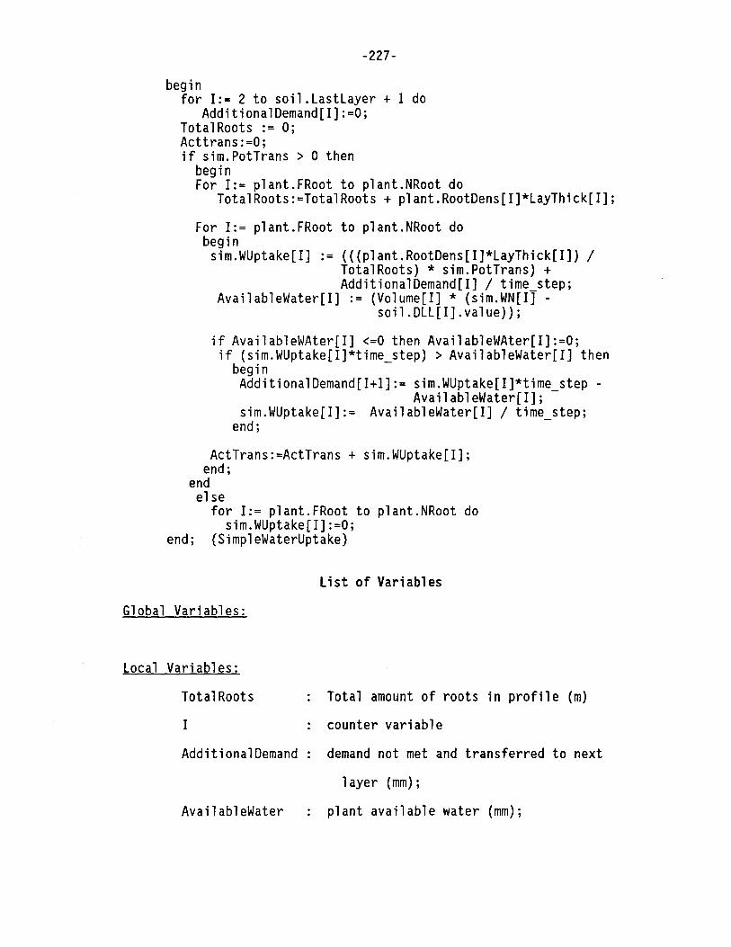
-227-

begin for I:= 2 to soil.Lastlayer + 1 do

AdditionalDemand[I]:=0; TotalRoots := O; Acttrans:=0; if sim.PotTrans > 0 then

begin For I:= plant.FRoot to plant.NRoot do

TotalRoots:=TotalRoots + plant.RootDens[I]*LayThick[I];

For I:= plant.FRoot to plant.NRoot do begin sim.WUptake[I] := (((plant.RootDens[I]*LayThick[I]) /

TotalRoots) * sim.PotTrans) + AdditionalDemand[I] / time step;

AvailableWater[I] :=(Volume[!]* (sim.WN[IJ -soil.DLL[I].value));

if AvailableWAter[I] <=0 then AvailableWAter[I]:=0; if (sim.WUptake[I]*time step) > AvailableWater[I] then

begin -AdditionalDemand[I+l]:= sim.WUptake[I]*time step -

AvailableWater[I]; -sim.WUptake[I]:= AvailableWater[I] / time step;

end; -

ActTrans:=ActTrans + sim.WUptake[I]; end;

end else

for I:= plant.FRoot to plant.NRoot do sim.WUptake[I]:=0;

end; {SimpleWaterUptake)

Global Variables:

Local Variables:

Total Roots

I

Additional Demand

AvailableWater

List of Variables

Total amount of roots in profile (m)

counter variable

demand not met and transferred to next

layer (mm);

plant available water (mm);

-228-

3.2.17 Procedure Soil_Temperature

The change in soil temperature over time will depend on the ability

of the soil to conduct heat and on the heat capacity of the soil. The

thermal conductivity of the soil is to a large degree a function of its

water content and bulk density.

In the procedure Estimate_Parameters four empirical coefficients

used to estimate the thermal properties are estimated. Coeff4 is the

thermal conductivity when soil.WN is zero and can be approximated by

(Campbell, 1985):

(1) Coeff4[I]:=0.3+0.1 * soil.BulkDensity[I] * soil.BulkDensity[I];

where: soil.BulkDensity is the bulk density (Mg m- 3 )

Coeff2 in part determines the differences in the thermal conductivity of

saturated soils and is dependent on the total volume fraction of soils

(Campbell, 1985):

(2) Coeff2[I]:=1.06 * soil.BulkDensity[I];

where 1.06 includes a correction for particle density, assuming a

particle density of 2.65 Mg m- 3 • Coeffl also in pert determines the

differences in thermal conductivity of saturated soils and is based on

work by DeVries (1963). The volume fraction of quartz is assumed to be

zero and the value for particle density is assumed as above:

(3) Coeffl[I]:=0.65-0.78*soil.BulkDensity[I] + 0.6* soil.BulkDensity[I]

* soil.BulkDensity[I]; I

Coeff3 determines the water content at which thermal conductivity

rapidly increases. This appears to be highly dependent on the clay

content of the soil:

(4) Coeff3[I]:= 1.0+2.6 / (SQRT(soil.clayPercent / 100));

-229-

where: soil.ClayPercent is percent clay of the soil

Once the coefficients are calculated in the procedure

Estimate_Parameters, thermal conductance and heat capacitance is

calculated for each layer in procedure Capacitance Conductance. The

heat capacitance (CP) is calculated multiplying the vulumetric specific

heats of soil and water with the volume fraction of mineral soil and

water, respectively:

(5) CP[I]:= (SpecHeatSoil * soil.BulkDensity[I] / soil.PartDensity[I]

+ SpecHeatWater * sim.WN[I]) * (LayThick[I]/time step);

where: SpecHeatSoil is the volumetric specific heat of soil {2.4 MJ m- 3 K-

1 )

SpecHeatWater is the volumetric specific heat of water (4.18 MJ m- 3 K-1)

soil.BulkDensity is the bulk density (Mg m- 3) soil.PartDensity is the particle density (Mg m- 3) LayThick is the layer thickness (m) time step is the time step (sec) sim.WN is the water content (rn3 m- 3)

The equation used to estimate the soil thermal conductance (K) for

any soil layer is taken from Mcinnes (1981):

(6) K[I] :=

where:

(Coeffl[I]+Coeff2[I]*sim.WN[I]-(Coeffl[I]-Coeff4[I]) *

EXP(-(POW((Coeff3[I]*sim.WN[I]),4)))) /

(soil.NodeDepth[I+l]-soil.NodeDepth[I]);

Coeffl - 4 are empirical coefficients related to soil water content and bulk density

sim.WN is the soil water content {m3 m-3) soil.NodeDepth is the soil node depth (m)

Since this equation is divided by the length of the soil layer to which

it applies, the conductivity becomes the conductance in this one

dimensional flow problem.

-230-

The procedure Boundary_Conditions specifies the upper and lower

boundary conditions used in the soolution to the heat flow problem.

Heat transfer from the surface of the soil to the air is assumed to be

directly dependent on the difference between air temperature and surface

soil temperature times a surface boundary conductance provided as input

(loca.BLC). The temperature at the bottom of the profile is kept

constant at the initial soil temperature for the last soil layer

(soil.InitSoilTemp[Lastlayer]) specified in the soil input file.

Heat fluxes are calculated by applying the equation of continuity

to the Fourier law:

d SoilTemp (7) CP * -------------- =

d time

d SoilTemp d ( K -----------------) / d NodeDepth

d NodeDepth

The numerical solution to this equation is similiar to the solution

of the water flow problem. First a Jacobian matric is formed in the

procedure Jacobian and then the procedure Thomas Algorithm uses the

Thomas Algorithm to solve a series of equations using Gauss elimination.

Since the conductances and capacitances are not a function of the

driving force as is the case in the water flow problem, no itterations

are needed to find the correct solution for the new soil temperatures.

After a new set of soil temperatures is calculated, procedure

Cale Fluxes calculates the heat flux (sim.HeatFlux) accross the soil

surface (positive downwards):

(8): sim.HeatFlux:=loca.BLC*(G*(sim.SoilTemp[l]-sim.SoilTemp[2]) +

loca.F*(TN[l]-TN[2]));

where: sim.SoilTemp[l] is the air temperature (°C) at last timestep

-231-

sim.Soi1Temp[2] is the surface node soil temperature (°C) at the last timestep

TN[l] is the air temperature (°C) at the next timestep TN[2] is the surface node soil temperature (°C) at the next

timestep loca.F is the weighing factor for the finite difference solution G is (1-loca.F) loca.BLC is the boundary layer conductance

List of References

Campbell, G.S. 1985. Soil Physics with BASIC. Elsevier, New York. 149 pp.

DeVries, D.A. 1963. Thermal properties of soils. p.210-235. In: vanWijk, W.R.(ed) Physics of Plant Environment. North-Holland Publishing Co., Amsterdam.

Mcinnes, K.J. 1981. Thermal conductivities of soils from dryland wheat regions of Eastern Washington. M.S. thesis, Washington State University, Pullman.


Procedure Soil Temperature; canst -

var

SpecHeatSoil = SpecHeatWater =

I G Coeffl

Coeff2 Coeff3 Coeff4 K CP TN

BGauss,CGauss, AGauss,DGauss:

2400000.0; 4180000.0;

integer; real; depth;

depth; depth; depth; depth; depth; depth;

depth;

procedure Capacitance Conductance; begin -

for I:= 2 to soil.Lastlayer do begin

{1-F} {coefficients to estimate thermal Cond}

{soil thermal conductance} {soil thermal capacity} {soil temperatures at new time step}

{partials in Jacobian matric}

CP[I]:= (SpecHeatSoil * soil.BulkDensity[I].value/

-232-

soil.PartDensity[I].value + SpecHeatWater * sim.WN[I]) * (LayThick[l]/time step);

K[I] := (Coeffl[I]+Coeff2[1]*sim.WN[I]-(Coeffl[I]-Coeff4[I]) *EXP(-(POW((Coeff3[I]*sim.WN[l]),4))))/ (soil.NodeDepth[I+l].value-soil.NodeDepth[l].value);

end; end; {Capacitance_Conductance}

procedure Boundary_Conditions;

begin G:=1-loca.F; K[l]:=loca.BLC; sim.SoilTemp[l]:=AirTemp; sim.SoilTemp[soil.Lastlayer+l]:=

soil.InitSoilTemp[soil.Lastlayer].value; TN[soil.Lastlayer+l]:=sim.SoilTemp[soil.LastLayer+l];

end;

procedure Estimate Parameters; begin -

for I:=2 to soil.Lastlayer do begin Coeffl[I]:=0.65-0.78*soil.BulkDensity[I].value+0.6 *

soil.BulkDensity[I].value*soil.BulkDensity[I].value; Coeff2[I]:=1.06*soil.BulkDensity[I].value; Coeff3[I]:=1.0+2.6/(SQRT(soil.clayPercent)); Coeff4[I]:=0.3+0.l*soil.BulkDensity[I].value *

soil.BulkOensity[I].value end;

end;

procedure Jacobian; begin

TN[l]:=AirTemp; For l:=2 to soil.Lastlayer do

begin CGauss[I]:=-K[I]*loca.F; AGauss[I+l]:=CGauss[I]; BGauss[I]:=loca.F*(K[I]+k[I-l])+CP[I];

DGauss[I]:=G*K[l-l]*sim.SoilTemp[l-l]+(CP[l]-G*{K[I]+k[I-1])) *sim.SoilTemp[I]+ G*K[I]*sim.SoilTemp[I+l];

end; DGauss[2]:=DGauss[2]+K[l]*TN[l]*loca.F;

DGauss[soil .Lastlayer]:=DGauss[soil.Lastlayer]+K[soil.Lastlayer]* loca.F*TN[soil.Lastlayer+I];

end;

procedure Thomas Algorithm; begin -

-233-

For I:=2 to soil.Lastlayer-1 do begin

CGauss[I]:=CGauss[I]/BGauss[I]; DGauss[I]:=DGauss[I]/BGauss[I]; BGauss[I+l]:=BGauss[I+l]-AGauss[I+l]*CGauss[I]; DGauss[I+l]:=DGauss[I+l]-AGauss[I+l]*DGauss[I];

end;

TN[soil.Lastlayer]:=DGauss[soil .Lastlayer]/BGauss[soil.Lastlayer]; {Back substitution} For I:=soil.Lastlayer-1 downto 2 do

TN[I]:=DGauss[I]-CGauss[I]*TN[I+I]; end; {Thomas_Algorithm}

procedure Cale Fluxes; begin -

sim.HeatFlux:=K[l]*(G*(sim.SoilTemp[l]-sim.SoilTemp[2]) +loca.F*(TN[l]-TN[2]));

For I:=2 to soil.Lastlayer+l do sim.SoilTemp[I]:=TN[I];

sim.SoilTemp[l]:=TN[l]; end;

begin {SoilTemperature} Boundary Conditions; Estimate-Parameters; Capacitance Conductance; Jacobian; -Thomas_Algorithm; Cale Fluxes;

end; {SoilTemperature}

Global Variables:

sim.SoilTemp

sim.HeatFlux

soil .BulkDensity

soil .PartDensity

soil.Lastlayer

soil.NodeDepth

soil.ClayPercent

List of Variables

soil temperature (°C)

surface heat flux (W m-2)

soil bulk density (Mg m-3)

soil particle density (Mg m-3)

last soil layer number

depth of soil layers (m)

percent clay fraction (%)

soil.InitSoilTemp

loca.BLC

loca.F

AirTemp

sim.WN

LayThick

Local Variables:

I

G

Coeffl

soil

Coeff2

Coeff3

Coeff4

K

CP

TN

BGauss,CGauss,

AGauss,OGauss:

Local Constants:

SpecHeatSoil

-234-

initial soil temperature (°C)

boundary layer conductance (20)

weighing factor, finite difference method (0 -

I)

air temperature (°C)

soil water content ( m3 m-3)

layer thickness (m)

counter variable

(1-loca.F)

coefficients to estimate thermal properties of

II

II

II

soil thermal conductance

soil thermal capacity

soil temperatures at new time step (°C)

coefficients in Jacobian matric

volumetric specific heat of soil (2.4 MJ m- 3 K

I)

SpecHeatWater

-235-

volumetric specific heat of water (4.18 MJ m- 3

K-1 ).

3.2.18. Const_Soil_Temperature

This procedure maintains the soil temperatures of each layer at the

initial value specified in the soil input file (soilinitSoilTemp[I]).

3.3 Linking modules

The attempt was made to design the procedures in a modular fashion

in order to exchange them as freely as possible and to keep them

compatible. Nevertheless, it is important to be aware of the input and

output requirements of the different procedures. Some require input

that necessitates implementing another procedure. To use the potential

driven Water_Uptake procedure to calculate plant water uptake, for

example, the Richards_Flow water flow procedure has to be selected,

since Tipping_Bucket_Flow does not produce soil water potentials as

output.

3.4 Run Time Plotting

A selected number of variables (up to four at a time) can be

plotted during the execution of a simulation run. To choose the

variables to be plotted, select option 'Procedures' from the GAPS

Simulator menu, then select 'View'. A list of variable names will

appear from which either one, two, or four can be selected to be plotted

-236-

on the screen. Simply scroll up and down the list and select by hitting

the 'Activate' key. 'Deactivate' disables a particular variable. After

a simulation comes to an end, the program will pause to give you a

chance to look at the finished plot or to screen dump it to the printer.

Hit <enter> to return to the GAPS Simulator menu.

3.5 Saving Output to Files

If desired, output data can be send to files on disk for later use.

At this time, GAPS does not allow you to specify which variables to

save. It will optionally create a summary output file, that will write

daily summary variables to disk, and also save information on the

particular implementation of a simulation run, such as input and output

file names and simulation procedures used. This file always carries the

extension *.SUM. Two other files will be created when data is to be

saved at the time step level. One file (*.EXl) contains the values of

variables that are a function of time and depth in the soil profile,

such as water content and water potential, water uptake from each soil

layer, soil water fluxes between each of the layers and soil

temperatures. Another file (*.EX2) contains only time dependent

information, such as current rates of evapotranspiration, drainage (from

the bottom of the profile), soil heat flux, and others. All three files

will be placed in the directory \GAPS\DATA. All three files will have

the same file name, but different extensions. These files can be used

in conjunction with plotting routines to obtain further output from the

model or they can be read into spreadsheets for further manipulation.

-237-

To save output data, select option 'Out' from the GAPS Simulator

menu. This will take you through a series of three menus. In the

first menu ('Hourly') you can select an already existing file from the

displayed list and overwrite it ('Load')or create a new file by

specifying a name (without file extension) and choosing 'Make'. Choose

'quit' if you don't want to save hourly data. The next window lets you

do the same for a daily output file, which will also contain information

on the simulation run configuration. The third window will allow you to

select a format for saving output, that you must have created previously

with the GAPS Editor (see Chp. 2.1.5). Output can be saved on selected

days and at selected hours during the day.

To get hard copies of the output files, access them via the GAPS

Plotter (Chpt. 4.3) or simply print them from DOS.

Documents

PREDICTING WATER CONSTRAINTS TO