PREDICTING U.S. STATE ADOPTION OF ENERGY EFFICIENCY RESOURCE STANDARDS

A Thesis submitted to the Faculty of the

Graduate School of Arts and Sciences of Georgetown University

in partial fulfillment of the requirements for the degree of

Master of Public Policy in Public Policy

By

Benjamin King, B.A.

Washington, DC April 18, 2014

ii

Copyright 2014 by Benjamin King. All Rights Reserved

iii

PREDICTING U.S. STATE ADOPTION OF ENERGY EFFICIENCY RESOURCE STANDARDS

Benjamin King, B.A.

Thesis Advisor: Micah K. Jensen, Ph.D.

ABSTRACT

In the absence of meaningful federal action, many states have adopted clean energy policies

aimed at reducing carbon emissions. Among these policies is the energy efficiency resource

standard (EERS), adopted by 33 states mostly in the last decade, which sets an energy

consumption reduction target for some or all regulated utilities within a state. My paper

examines what factors affect a state’s likelihood of adopting an EERS, and whether those factors

are different for EERS policies compared with other clean energy policies. The energy policy

literature features many studies of clean energy policy adoption, but none have focused

specifically on EERS adoption. I theorized that energy efficiency potential being relatively

homogeneously distributed across states (compared to renewable energy potential) and

efficiency’s relative inexpensiveness as a resource would result in a unique set of factors being

associated with the likelihood of EERS adoption. Specifically, I expected that three internal

determinants—the presence of utility rate decoupling in a state, a state’s political ideology, and

the state’s average retail price of residential electricity—affect a state’s likelihood of adopting an

EERS. To test these hypotheses, I estimated several multiple regression models using an event

history analysis approach and found that citizen liberalism, level of electricity consumption, and

a time counter variable were all statistically significant and positive predictors of state adoption

iv

of an EERS, all else equal. I found no association between decoupling or electricity price and

EERS adoption, though in the case of the former that may be a result of insufficient data.

v

ACKNOWLEDGEMENTS

Many thanks to the faculty and students of the McCourt School of Public Policy for creating an environment so conducive to learning. Thanks in particular to my thesis advisor, Micah Jensen,

who provided a wealth of critical guidance along the way while always emphasizing that it is my name on the final product.

I also want to express my sincere gratitude to my friends and family, who have been so

encouraging throughout the thesis process and my graduate school career more broadly. Thank you to Sean, who talked me into grad school in the first place. Thank you to Nicole, who endured

endless hours of discussions about energy policy and without whom I would not have made it through these last few years. Finally, thank you to my parents, who not only provided massive

amounts of support but who also serve as examples toward which I strive every day.

I am deeply grateful to each of you.

vi

TABLE OF CONTENTS

 INTRODUCTION ........................................................................................................................... 1  LITERATURE REVIEW ................................................................................................................ 3  

ENERGY EFFICIENCY RESOURCE STANDARDS .......................................................................................... 4  STATE CLEAN ENERGY POLICY ADOPTION .............................................................................................. 6  EXPLAINING POLICY ADOPTION ............................................................................................................. 10  

CONCEPTUAL MODEL AND HYPOTHESES ......................................................................... 14  METHODS .................................................................................................................................... 16  

DATA ............................................................................................................................................ 19  BIVARIATE CORRELATIONS ..................................................................................................................... 24  

RESULTS ...................................................................................................................................... 26  DISCUSSION ................................................................................................................................ 32  

CONCLUSION ............................................................................................................................. 37  APPENDIX ................................................................................................................................... 39  

REFERENCES .............................................................................................................................. 44  

1

INTRODUCTION

In an oft-cited quote from New State Ice Co. v. Liebmann (1932, p. 23), Justice Louis

Brandeis posited that states may “serve as a laboratory; and try novel social and economic

experiments.” This certainly appears to be the case within the realm of clean energy policy. With

the inability of Congress to pass meaningful clean energy legislation at the federal level in recent

years, many states have taken up the cause and adopted a variety of policies seeking to reduce

carbon emissions produced by their electric power generation sectors and increase the

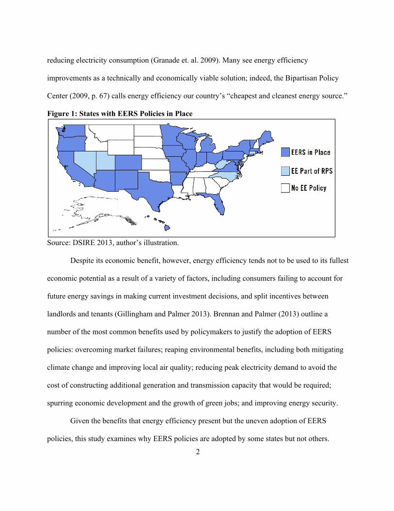
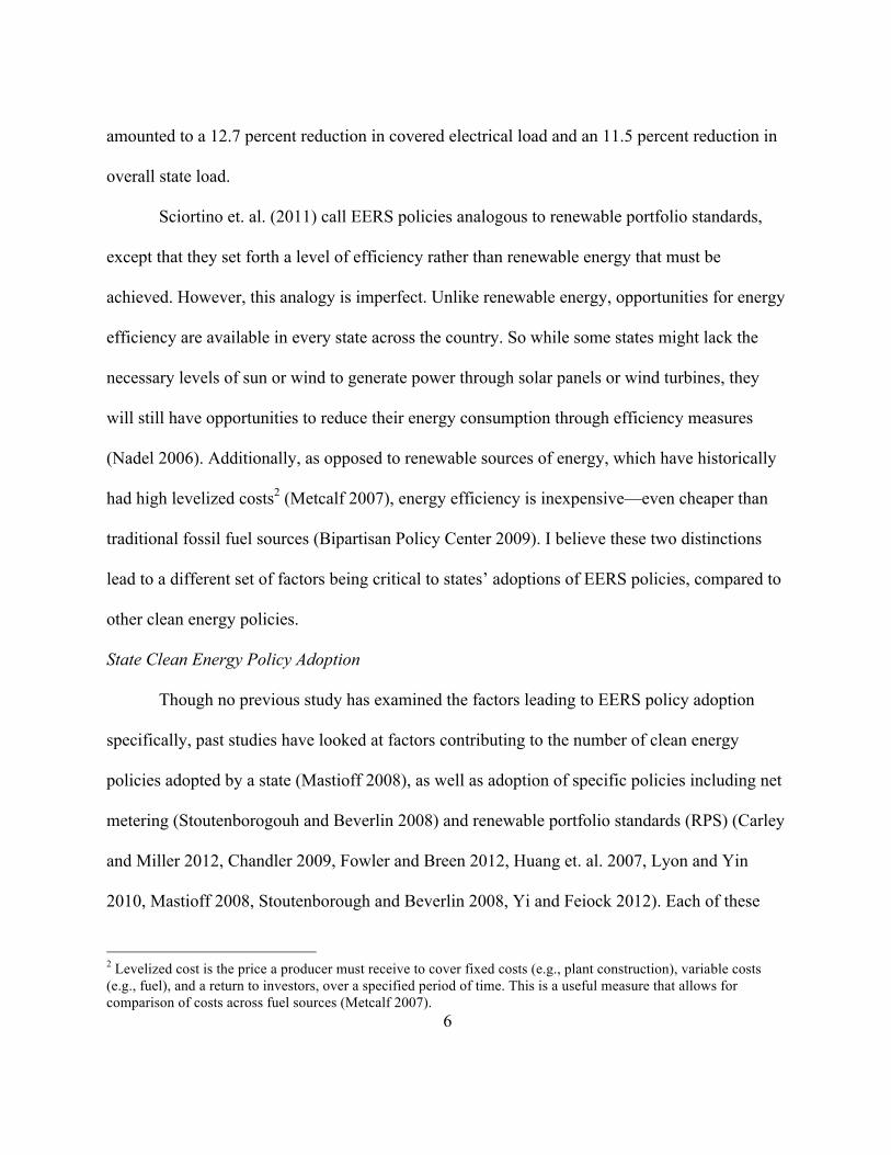
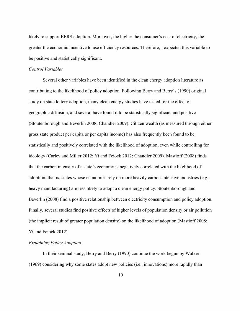
deployment of renewable energy (Carley 2011). One such policy is the energy efficiency

resource standard (EERS), which sets an energy savings target for regulated utilities and has

been adopted in some form in 33 states, as demonstrated in Figure 1 (Nadel 2006; Database of

State Incentives for Renewables and Efficiency (DSIRE) 2013). For example, Arizona’s Energy

Efficiency Standard calls for the state’s regulated electric utilities to achieve a 22-percent

reduction in retail sales over their 2010 level by 2020 (DSIRE 2013). This paper examines what

factors lead states to adopt EERS policies for electric utilities1 and considers whether distinctions

in energy efficiency provisions, compared with clean energy policy writ large, lead to different

factors being significant.

Policies to promote reductions in energy consumption came into vogue in the 1970s, but

tended to focus on specifying a level of funding for energy efficiency programs rather than

setting a specific and measurable percentage or quantity reduction in electricity demand (Nadel

2006). Recently, rising concerns about energy prices, energy security, and climate change have

led to an increasing consideration of energy efficiency as a way to address these problems by

1 Many of these states have EERS policies in place for their natural gas utilities as well, but those policies are outside the scope of this paper.

2

reducing electricity consumption (Granade et. al. 2009). Many see energy efficiency

improvements as a technically and economically viable solution; indeed, the Bipartisan Policy

Center (2009, p. 67) calls energy efficiency our country’s “cheapest and cleanest energy source.”

Figure 1: States with EERS Policies in Place

Source: DSIRE 2013, author’s illustration.

Despite its economic benefit, however, energy efficiency tends not to be used to its fullest

economic potential as a result of a variety of factors, including consumers failing to account for

future energy savings in making current investment decisions, and split incentives between

landlords and tenants (Gillingham and Palmer 2013). Brennan and Palmer (2013) outline a

number of the most common benefits used by policymakers to justify the adoption of EERS

policies: overcoming market failures; reaping environmental benefits, including both mitigating

climate change and improving local air quality; reducing peak electricity demand to avoid the

cost of constructing additional generation and transmission capacity that would be required;

spurring economic development and the growth of green jobs; and improving energy security.

Given the benefits that energy efficiency present but the uneven adoption of EERS

policies, this study examines why EERS policies are adopted by some states but not others.

3

There is a growing body of literature that provides potential answers to this question for a variety

of other clean energy policies, but no study has considered EERS policies specifically. Though

EERS policies have been called analogous to renewable portfolio standards (Sciortino et. al

2011) and aim to achieve similar goals as other clean energy policies, I believe there are several

key distinctions between policies that promote energy efficiency and those that promote

renewable energy or clean energy more broadly. These distinctions lead to a different set of

factors being critical to states’ adoption of EERS policies.

EERS policies (or an equivalent policy) have been adopted in 33 states, but 17 states and

the District of Columbia have not yet adopted such a policy. By understanding what factors lead

states to adopt EERS policies, energy efficiency policy advocates might adjust the design of

these policies so that they can be adopted in other states, helping continue to shrink our national

carbon emissions. Especially since the opportunities for energy efficiency gains are distributed

widely across the states, adopting EERS policies in these 18 remaining states could be helpful in

reducing our country’s overall electricity consumption, as EERS policies have generally been

seen as effective in doing so (Sciortino et. al. 2011; Carley and Browne 2013). Additionally,

such an understanding might illuminate a path toward successful adoption of energy efficiency

policies at the national level.

LITERATURE REVIEW

Though the existing literature has not specifically examined the factors leading to state

adoption of EERS policies, a fair amount of writing exists on both the structure of and

justifications for EERS adoption. Moreover, there is a growing body of literature that examines

4

state adoption of a variety of other clean energy policies, finding chiefly that liberalism and

renewable energy potential are the main factors leading to such events.

Energy Efficiency Resource Standards

At the most basic level, an EERS policy sets a target reduction in energy use for utilities

within a given state (i.e., a set percent or quantity reduction in retail sales over a specified base

year by a given year in the future.) These utilities then use a variety of financial incentives and

regulations to motivate lower levels of energy consumption by their customers, thus achieving

these reductions (Nadel 2006). Though the first EERS was adopted in Florida in 1980, the

remaining 32 states that have adopted an EERS or EERS-like policy have done so since 1997,

with 23 adoptions happening since 2007 (DSIRE 2013).

Though improving energy efficiency often makes economic sense for electricity end

users, many times consumers fail to adjust behavior or purchase technologies to capture this

benefit. This tendency is referred to as the energy efficiency gap. Gillingham and Palmer (2013)

conducted a comprehensive review of the literature and identified a variety of market failures as

causes of this gap. Consumers may have imperfect information regarding the level of savings

that could result from efficiency improvements, they may not properly value future energy

savings in making present investments, they may not have access to the necessary credit to

finance these investments, or they may face a distorted price of electricity that understates its true

cost. Particularly for renters (both residential and commercial), split incentives may also play a

role, wherein landlords would typically be the party to pay for efficiency improvements to the

homes or buildings they own but, since tenants tend to pay the utility bills, landlords have no

incentive to make these investments.

5

The result, as in many cases of market failure, is that government policy is needed to

drive energy efficiency. EERS policies are adopted for a variety of reasons: environmental

benefits, including both mitigating climate change and improving local air quality; reducing peak

electricity demand to avoid the cost of constructing additional generation and transmission

capacity that would be required; addressing the broader market barriers that lead consumers

generally to underinvest in efficiency; spurring economic development and the growth of green

jobs; and improving energy security (Brennan and Palmer 2013). Regulatory frameworks, which

include EERS policies, have helped elevate energy efficiency in utility business models and, as a

result, utilities in this country spent $5.9 billion on efficiency programs in 2012 (York et. al.

2013).

Despite being grouped under the EERS policy label, there is a great deal of variation in

the way these policies are designed and implemented across states. Palmer et. al. (2013) detail

these differences across 19 EERS policies. States vary in which of their regulated utilities are

included in the policy (e.g., investor-owned utilities only versus all utilities including municipal

utilities and rural co-ops.) States also vary in their reduction targets: some have annual

percentage reduction goals (e.g., 3 percent per year in Pennsylvania); others have cumulative

percentage goals (e.g., Arizona aims to reduce their energy use by 22 percent by 2020); still

others set annual or cumulative quantity reduction goals (e.g., a 189 gigawatt-hour reduction in

demand by 2014 in Rhode Island). Palmer et. al. (2013) collect these targets across the 19 states

they examine, standardize them all into a cumulative quantity reduction, and determine the

percent of each state that is covered under the EERS. All told, the 19 policies they examined

6

amounted to a 12.7 percent reduction in covered electrical load and an 11.5 percent reduction in

overall state load.

Sciortino et. al. (2011) call EERS policies analogous to renewable portfolio standards,

except that they set forth a level of efficiency rather than renewable energy that must be

achieved. However, this analogy is imperfect. Unlike renewable energy, opportunities for energy

efficiency are available in every state across the country. So while some states might lack the

necessary levels of sun or wind to generate power through solar panels or wind turbines, they

will still have opportunities to reduce their energy consumption through efficiency measures

(Nadel 2006). Additionally, as opposed to renewable sources of energy, which have historically

had high levelized costs2 (Metcalf 2007), energy efficiency is inexpensive—even cheaper than

traditional fossil fuel sources (Bipartisan Policy Center 2009). I believe these two distinctions

lead to a different set of factors being critical to states’ adoptions of EERS policies, compared to

other clean energy policies.

State Clean Energy Policy Adoption

Though no previous study has examined the factors leading to EERS policy adoption

specifically, past studies have looked at factors contributing to the number of clean energy

policies adopted by a state (Mastioff 2008), as well as adoption of specific policies including net

metering (Stoutenborogouh and Beverlin 2008) and renewable portfolio standards (RPS) (Carley

and Miller 2012, Chandler 2009, Fowler and Breen 2012, Huang et. al. 2007, Lyon and Yin

2010, Mastioff 2008, Stoutenborough and Beverlin 2008, Yi and Feiock 2012). Each of these

2 Levelized cost is the price a producer must receive to cover fixed costs (e.g., plant construction), variable costs (e.g., fuel), and a return to investors, over a specified period of time. This is a useful measure that allows for comparison of costs across fuel sources (Metcalf 2007).

7

papers has considered at least state internal determinants or geographic diffusion as relevant

factors in clean energy policy adoption.

One of the most consistent findings to come out of these studies is that some form of

renewable energy potential is often a factor that increases the likelihood of clean energy policy

adoption (Lyon and Yin 2010, Mastioff 2008, Stoutenborough and Beverlin 2008, Yi and Feiock

2012). This result makes sense, as those states with more potential face less of an economic

obstacle in increasing renewable deployment and, thus, should be more likely to embrace

policies that make this a goal. Compared with renewable energy potential, energy efficiency

potential is much more homogenous across states, especially when controlling for the size of the

state’s economy. There is also no widely acknowledged and systematic operationalization of

efficiency potential. Thus, understanding what factors contribute to policy adoption in the

absence of a meaningful measure of potential is a partial motivation for my paper.

Electricity Rate Decoupling3

Under the traditional electric utility model, utility customers pay a set rate, negotiated

between the utility and the state’s public utility commission (or the equivalent). This rate consists

of a fixed customer cost plus a variable cost that depends on the amount of electricity the

customer consumes. To earn the reasonable returns (i.e., profit) they have been guaranteed under

their existing rate structure, the utility must sell a certain amount of electricity. This business

model provides a disincentive for the utility to pursue energy efficiency, as selling less electricity

hurts their bottom line.

3 I am grateful to David Gardiner for suggesting the role that decoupling could play in utility acceptance of EERS policies.

8

A decrease in sales is not the only way that efficiency impacts utilities financially.

Energy efficiency programs also cost utilities money to design and implement, though these

costs tend to be easily recovered through subsequent rate cases. More challenging, increasing

energy efficiency decreases the need to invest in more power plants or other utility assets, but

utilities are often granted increased returns in rate cases as a result of making these large capital

expenditures.

Decoupling breaks this link between level of sales and profit and allows electricity rates

to adjust between rate cases so that utilities are ensured their reasonable returns regardless of

their kilowatt-hour sales (Sullivan et. al. 2011). While in a traditional model utilities are expected

to be hostile to EERS adoption, Croucher (2011) asserts that decoupled utilities are likely to not

oppose—and may even embrace—EERS policies. Croucher cites the fact that a majority of states

that allow decoupling also have an EERS as proof of this notion. I tested this by examining the

effect of decoupling while controlling for other relevant variables, expecting his assertion to

hold. Perhaps decoupling can be thought of as a sort of EERS potential, since a lack of utility

opposition makes it easier for states to adopt an EERS policy.

Liberalism

Even more frequently than renewable energy potential, past studies on clean energy

policies have highlighted some measure of liberalism as a factor contributing to policy adoption,

as more liberal states tend to support greener policies. In their studies examining state RPS

adoption, both Carley and Miller (2012) and Yi and Feiock (2012) control for both the ideology

of a state’s citizens and its government officials (using the Berry et. al. (1998, 2010) measures I

detail below) and find that citizen ideology is positively associated with adoption, meaning the

9

more liberal a state’s citizenry, the more likely they are to adopt an RPS policy. Carley and

Miller also find the government ideology statistically significant in the adoption of the most

stringent forms of RPS policies. Mastioff (2008) likewise (and using the same measure) finds

citizen ideology statistically significant in his study on RPS adoption, though he does not control

for government ideology. Stoutenborough and Beverlin (2008) find that government ideology is

statistically significantly associated with net metering adoption (again using the Berry et. al.

measure), even when controlling for a state’s green conditions, which they use as a proxy for the

level of environmentalism in a state. In other studies, Fowler and Breen (2012) find that the

number of Democratic members of a state’s lower house and upper house are statistically

significantly associated with RPS adoption; Lyon and Yin (2010) similarly find percentage of

Democrats in the state legislature is associated with RPS adoption. Finally, Huang et. al. (2007)

find that states where Republicans dominate the legislature are less likely to adopt an RPS.

Though the lower cost of implementing energy efficiency measures could mean that marginally

less liberal states become more likely to adopt an EERS policy, I believed that liberalism would

still be an important factor in these policy adoptions.

Retail Price of Electricity

One factor that has been controlled for in previous clean energy adoption studies, but not

found to be statistically significant, is the retail price of electricity (Carley and Miller 2012, Lyon

and Yin 2010). Given that renewable energy tends to be more expensive than the fossil fuel

sources clean energy policies seek to replace, this result makes intuitive sense. Since energy

efficiency is a less expensive resource than traditional fossil fuel sources, I expected that

consumers would want to increase their use of energy efficiency and, therefore, would be more

10

likely to support EERS adoption. Moreover, the higher the consumer’s cost of electricity, the

greater the economic incentive to use efficiency resources. Therefore, I expected this variable to

be positive and statistically significant.

Control Variables

Several other variables have been identified in the clean energy adoption literature as

contributing to the likelihood of policy adoption. Following Berry and Berry’s (1990) original

study on state lottery adoption, many clean energy studies have tested for the effect of

geographic diffusion, and several have found it to be statistically significant and positive

(Stoutenborough and Beverlin 2008; Chandler 2009). Citizen wealth (as measured through either

gross state product per capita or per capita income) has also frequently been found to be

statistically and positively correlated with the likelihood of adoption, even while controlling for

ideology (Carley and Miller 2012; Yi and Feiock 2012; Chandler 2009). Mastioff (2008) finds

that the carbon intensity of a state’s economy is negatively correlated with the likelihood of

adoption; that is, states whose economies rely on more heavily carbon-intensive industries (e.g.,

heavy manufacturing) are less likely to adopt a clean energy policy. Stoutenborough and

Beverlin (2008) find a positive relationship between electricity consumption and policy adoption.

Finally, several studies find positive effects of higher levels of population density or air pollution

(the implicit result of greater population density) on the likelihood of adoption (Mastioff 2008;

Yi and Feiock 2012).

Explaining Policy Adoption

In their seminal study, Berry and Berry (1990) continue the work begun by Walker

(1969) considering why some states adopt new policies (i.e., innovations) more rapidly than

11

others. Berry and Berry seek to combine two distinct methods of policy research into one model.

In examining why some states adopt state lotteries, they consider both internal determinants

(e.g., economic, social, and political characteristics unique to each state) and regional diffusion

(e.g., states being influenced by what their neighbors are doing), using event history analysis.

The authors unite these two trends of study under Mohr’s (1969) theory of organizational

innovation, in which he posits that the propensity to innovate is a function of motivation, how

strong the forces pushing against innovation are, and what resources are available to counteract

such forces.

Berry and Berry (1990) consider a variety of factors that could motivate states to adopt a

lottery within this framework: the state’s fiscal health and election calendar (Mohr’s motivations

to innovate); personal income and the percentage of a state’s residents that subscribe to a

fundamentalist religion (Mohr’s strength of obstacles to innovation); and whether there is unified

control of government and how many neighboring states had previously adopted a lottery

(Mohr’s availability of resources to overcome obstacles). The authors use a binary dependent

variable indicating whether a state adopted a lottery in a given year and find that all their

explanatory variables are statistically significant at varying levels except the state’s fiscal health,

providing proof of concept for a unified model that simultaneously considers internal

determinants and regional diffusion.

In a later article, Berry and Berry (2007) provide additional theoretical justification for

the influence of geographic diffusion on policy adoption. The authors outline three basic reasons

that policies may diffuse in a neighborwise fashion: states may learn from watching one another

and implement policies that have been successful in other states; they may compete with each

12

other to attract jobs or firms or otherwise gain an economic advantage; or they may feel the need

to conform to a nationally or regionally accepted standard. Under a regional diffusion model

(such as the one used in their 1990 article), states are assumed to be influenced by their

neighbors more readily than states more geographically further afield because learning is easier

to analogize in proximate states and because economic competition with states is fiercer among

neighbors because of constraints on the mobility of most individuals and firms.

Mooney (2001) delves deeper into the mechanics of geographic diffusion, as he believes

the process behind such diffusion has not been theoretically supported. Mooney highlights two

important sources of bias on the regional effect variables. First, he asserts the slope estimates on

the neighbor variable are biased toward the coefficient because the hazard rate is not constant

across time; to fix this, he proposes including a time trend variable or annual dummies. Second,

he further allows the effect of diffusion to vary over time through several alternate specifications

of Berry and Berry’s (1990) model on state lottery adoption. Rather than simply using the

number of the state’s neighbors as an explanatory variable, he calculates the average proportion

of adjacent adopters, which accounts for what percentage of a state’s neighbors had adopted the

policy weighted by the overall percentage of states nationally that had adopted the policy. Using

this variable, he finds the point at which neighbor adoption seems to start having diminishing

returns on the likelihood of adoption, and includes a dummy variable that is set to one for all

adoptions after this point. He interacts this new dummy with the number of adoptee neighbors to

allow for an intercept shift. He also includes a quadratic term on the number of neighbors (and

the new interacted term) to further allow for the effect of neighbor adoption to vary over time.

The result of these specification adjustments to Berry and Berry’s original model confirms their

13

finding of a positive coefficient on neighbor adoption, but only to a point, with diminishing

returns on successive adoptions afterwards. Mooney explains this result by suggesting that early

adoptions by states of untested policies have a greater impact on neighbors but that, as policy

diffuses and there is less uncertainty surrounding the policy’s effects, the value of seeing a

neighbor adopt the policy is diminished and might even be negative (if the effects of the policy

are seen as undesirable.)

Also using Berry and Berry (1990) as a starting point, Buckley and Westmoreland (2004)

tackle several important modeling issues in discrete event history analysis that were unaccounted

for in the original state lottery model. Berry and Berry’s original model assumes no change in the

hazard rate over time once the other variables in the model are controlled for (i.e., no durational

dependence). Like Mooney, the authors propose two potential solutions to solve this problem

with the model: either include a set of time dummy variables for t-1 time periods or include time

itself as a regressor (in the form of a time counter variable). Second, most studies that have used

event history analysis do not fully consider the impact of the choice in functional form. Changing

the Berry and Berry model from a probit to a logit has an effect on both the statistical

significances and coefficient estimates of several variables, since the logit function is more

heavily distributed as it approaches its limits (i.e., has fatter tails) compared to the probit

function. These tails matter because adoption is a very rare event in most datasets. Instead of

either of these more common forms of binary dependent variable models, Buckley and

Westmoreland suggest that the complementary log-log (cloglog) form is more appropriate for

rare events like policy adoption since it is asymmetrical, with more of its distribution shifted

leftward, allowing for rare adoptions to be captured in its thinner right tail.

14

Based on the foregoing review of the literature, I concluded that using an event history

analysis approach for my model to examine which factors lead to states adopting EERS policies

is appropriate. Moreover, studies on EERS and other clean energy policies suggest a set of

factors that are likely to be relevant to EERS adoption, including state liberalism, whether

electricity rate decoupling exists in a state, and the state’s retail price of electricity.

CONCEPTUAL MODEL AND HYPOTHESES

As outlined in my literature review, previous studies have examined the adoption of a

wide variety of clean energy policies, both individually and as a class of policies within a state;

however, none has examined state-level adoption of EERS policies specifically. I believe this is a

relevant research question because certain characteristics of energy efficiency policies (i.e.,

efficiency’s relative cheapness compared to renewables and the lack of a measure of efficiency

potential across states) are likely to lead to different factors being significant to policy adoption.

My conceptual framework predicts state EERS adoption as a vector of my three

explanatory variables of interest, namely electric rate decoupling, state liberalism, and retail rate

of residential electricity, and relevant control variables based on the preceding literature review,

as follows:

Pr(EERS Policy Adoption=1)k,t= β0 + β1(Decouplingk,t) + β2(Ideologyk,t) +

β3(Retail Price of Electricityk,t) + β4(Neighbor State Adoptionk,t-1) + β5(Carbon

Intensityk,t) + β6(Citizen Wealthk,t) + β7(Electricity Consumptionk,t) +

β8(Population Densityk,t) + β9(Time Countert) + uk,t

My dependent variable was an indicator identifying whether state k adopts an EERS

policy in year t. I proposed that three internal determinants would be statistically significant

15

contributors to state adoption of EERS policies, while controlling for several other factors that

have previously been identified to contribute to clean energy policy adoption.

First, I expected to find that states that allow for utility rate decoupling would be more

likely to adopt an EERS policy, all else equal. Since this decoupling allows utilities to continue

to be profitable while also promoting energy efficiency, they would be less likely to oppose the

state’s adoption of an EERS policy, and may even embrace such a policy. Therefore, my first

hypothesis was:

H1: Utility rate decoupling in a state is a useful predictor of whether a state

adopts an EERS policy.

H0: Utility rate decoupling is not a useful predictor of EERS adoption.

Second, previous studies have consistently found a statistically significant and positive

relationship between a state’s political ideology and its likelihood of clean energy policy

adoption. Though I expected that the lower cost of implementing energy efficiency compared

with renewable energy could lessen the strength of this relationship, I also expected that ideology

would still be an important factor in these policy adoptions, all else equal. Therefore, my second

hypothesis was:

H2: A state’s ideology is a useful predictor of whether it adopts an EERS policy.

H0: State ideology is not a useful predictor of EERS adoption.

Third, I expected that higher retail prices of residential electricity would make a state

more likely to adopt an EERS policy, all else equal. Here again I expected that the relative lower

cost of energy efficiency would have an impact: previous studies have not found a statistically

significant relationship between electricity price and policy adoption, but the high cost of

16

renewable energy could explain that result. Conversely, energy efficiency is relatively

inexpensive, and embracing efficiency has the potential to lower a consumer’s electricity bill.

Thus, the higher the consumer’s current bill, the greater the incentive to use efficiency resources

to save money. I therefore expected a different outcome than previous studies that have

examined this relationship. Thus, my third hypothesis was:

H3: State average retail rate of residential electricity is a useful predictor of

whether a state adopts an EERS policy.

H0: Average retail rate of residential electricity is not a useful predictor of EERS

adoption.

METHODS

The main analytic tool that has been used in studies of state policy adoption is event

history analysis (EHA) (Boehmke and Skinner 2012; Box-Steffensmeier and Jones 2004). As

Allison (1984) outlines in his excellent primer on the subject, EHA is concerned with some

relatively sudden change of states (an event) by an individual or group that occurs in a given time

period. Chiefly, EHA seeks to understand an individual or group’s hazard rate (i.e., the

probability of an event for a given individual). Though the hazard rate is unobserved, Allison

(1984, p. 16) calls it “the fundamental dependent variable in an event history model.”

To estimate a discrete-time hazard rate EHA model (such as is required for understanding

state policy adoption), data is collected for each individual or group in the risk set (i.e., the

collection of individuals or groups who are at risk of an event) for each discrete time period (e.g.,

year, month, day, etc.) over a given time period. The dependent variable is binary, coded as 1 if

the observation changes states in the specific discrete time period and 0 otherwise. Both time-

17

variant and time-invariant explanatory variables can be added to the model. The data is then

pooled across all years of interest and a regression (typically using the logit or probit form) is

estimated (Allison 1984).

As a statistical method, EHA seeks to address the difficulties of censored data, for

example cases where the individual or group does not change states within the arbitrary time

period of the study, and time-variant explanatory variables, which create problems for regression

and other typical statistical tools. Allison (1984, p. 19) argues EHA addresses the problem of

censoring by letting any individual or group contribute “exactly what is known about them,

namely that they did not change [states]” over the period of study. Moreover, the issue of time-

variant explanatory variables is moot, as each observation is for a separate year. Non-normal

distribution of events in a sample also violates a key assumption of standard regression analysis,

which can be addressed by substituting an alternate functional form, discussed in greater detail

below (UCLA: Statistical Consulting Group 2014).

To test my hypotheses, I estimated regression models using this discrete-time hazard rate

event history analysis approach, regressing my dependent variable, whether a state adopts an

EERS policy in a given year, on the explanatory and control variables I have outlined above.

Since my dependent variable was binary, a logit or probit model would have been appropriate.

However, as discussed above, Buckley and Westmoreland (2004) suggest that the

complementary log-log (cloglog) functional form could also be appropriate. Its associated

probability distribution is asymmetrically distributed, with relatively more area under the curve

as it approaches its lower bound than its upper bound. Policy adoption is a rare event, especially

since states are dropped from the dataset once they adopt a policy (only 26 observations out of

18

my full sample of 661 have a value of 1 in the dependent variable), so this distribution has the

potential to be a better fit. Buckley and Westmoreland also argue that the difference in the

distribution of the probit and logit curves can also have a significant impact on the outcome.

Therefore, I tested my model across all three functional forms to see if my results were

substantively consistent.

Stoutenborough and Beverlin (2008) review the relevant literature and deem fixed effects

inappropriate for time series models with binary dependent variables. Following their

recommendation, I instead used random effects to allow for varying intercepts for each panel

member. I also included a time trend variable to allow the hazard rate to vary across my sample.

Finally, as suggested in Mooney (2001), I included a variable that is the square of the number of

neighbors who adopted an EERS policy to allow for the potential of diminishing returns of

geographic diffusion.

Because my model’s dependent variable is binary, it was also critical to run a set of

postestimation tests. I was chiefly concerned with examining the effects of changes in my three

main explanatory variables at theoretically interesting sets of covariate values. For example,

what is the effect of increasing levels of liberalism at low retail rates of electricity versus high

retail rates of electricity, or what is the impact of decoupling electric rates at various levels of

ideology? To examine these questions, I estimated the average marginal effect of the variable of

interest while specifying values for some covariates and holding the other covariates as observed

in the sample.

19

DATA

I assembled data from several sources (outlined below) for all fifty states4 for the years

1996 through 2010,5 unless otherwise noted. Accounting for variables with missing data, my

overall valid sample size was 661 state-year observations.

Dependent Variable: EERS Adoption

My dependent variable was an indicator, set to 1 if a state adopted an EERS policy in the

specified year and 0 otherwise. Dates of adoption are drawn from the Database of State

Incentives for Renewables and Efficiency (DSIRE 2013) page for each state’s EERS policy. As

outlined above, both Sciortino et. al. (2011) and Palmer et. al. (2013) point out that there are key

distinctions between the EERS policies adopted across the states. Sciortino et. al. (2011)

differentiate states’ policies in terms of whether they are tailored to individual utilities or are

uniform statewide and whether efficiency contributes as part of a state’s renewable portfolio

standard rather than meeting a standalone target. In their study comparing EERS policies, Palmer

et. al. (2013) differentiate between states whose EERS targets are legally binding and not; they

also separate those states whose efficiency targets are part of their renewable portfolio standard

(RPS).

Since a central tenant of my theory is that EERS adoption has fundamentally different

characteristics than other clean energy policy adoption, particularly RPS adoption, I initially

wanted to consider only states that have standalone EERS targets (i.e., efficiency targets that are

not part of an RPS policy) as having adopted an EERS policy; thus states with efficiency only as

4 I excluded the District of Columbia because data regarding its ideology is not available from the source I used. 5 Oklahoma adopted an EERS policy in 2012 (DSIRE 2013), but much of the data I utilize is not yet available for that year; therefore, I end my analysis in 2010, the year of the next most recent adoption.

20

part of their RPS are excluded from my dataset.6 I also excluded Florida from my dataset as their

EERS was adopted during a previous generation of efficiency efforts (in 1980) and therefore is

likely to have been influenced by different factors than the current generation of efficiency

efforts. Finally, there was the question of those states that adopted a distinct EERS policy but did

so concurrently with either a separate RPS or some other energy policy (e.g., electric sector

restructuring, net metering, interconnection standards, etc.)7 I tested my model two ways:

considering these states as having adopted an EERS or dropping these five states from the

dataset entirely. I compared the results of these two regressions to determine the impact of this

specification decision. Of the 33 states that have EERS policies or similar efficiency targets, this

approach examined adoption in 26 states and 21 states, respectively.

Independent Variables: Decoupling

Morgan (2012) presents a state-by-state review of decoupling policies, indicating both

which states have adopted decoupling policies for one or more of their electric utilities and in

what year each decoupling took place. Based on her through review, I coded decoupling as an

indicator, set to 1 if a state either adopted electric rate decoupling for at least one utility in a

given year or had adopted decoupling in any previous year, and 0 otherwise.

Liberalism

Several clean energy adoption studies measure liberalism by making use of the Berry,

Ringquist, Fording, and Hanson (1998) measure of citizen ideology and the Berry, Ringquist,

Fording, Hanson, and Klarner (2010) measure of government ideology. I followed this example 6 The states that fall into this category are Connecticut, North Carolina, Nevada, Utah, and West Virginia. 7 These states are Michigan, Ohio, Texas, Virginia, and Washington.

21

in my study, as it appears to be a valid operationalization of this concept. Citizen ideology is a

score based on interest group ideological scores for members of Congress and their challenger

(or hypothetical challenger), weighted by biennial Congressional election results, which is then

aggregated at the state level to compute an unweighted average for the state as a whole.

Government ideology is generated through a similar process based on ideological scores, but

these scores are derived from a member or challenger’s NOMINATE common space coordinates

rather than interest group ratings and are further weighted by partisan balance in the state

legislature. Fording (2012) provides regularly updated scores on his website, which I used in this

paper.

Average Retail Price of Residential Electricity

The Energy Information Administration (2013) conducts an annual survey of electric

utilities, which includes a variety of data on consumption, generation, and price. Among these

data is the retail rate of electricity for residential consumers, which EIA subsequently aggregates

at the state level and reports in cents. EIA provides the responses to this survey question dating

back to 1990 on their website.

Adoption by Neighbors

Using the same DSIRE (2013) data referenced above, I generated the number of each

state’s neighbors that adopted an EERS policy in the prior year or earlier. In my

operationalization of the variable, Alaska is considered a neighbor of Washington and Hawaii is

considered a neighbor of California. For this variable, I considered all 26 states discussed above

as having a policy in place, plus I considered Florida as having a policy in place for the entire

22

year range. I did not consider those five states that have efficiency targets only as part of their

RPS as having an EERS policy in place for the purposes of this variable.

Other Control Variables

I collected state population data from the U.S. Census Bureau’s (2012) Intercensal

Population Estimates and gross domestic product by state (reported in chained 2005 dollars)

from the Bureau of Economic Analysis (n.d.). Using these two variables, I generated gross state

product per capita by dividing gross state product by the state population. To generate a state’s

population density, I divided state population by the state area (in square miles) as reported in the

Census Bureau’s (n.d.) State and County QuickFacts, generating a measure of people per square

mile. From the Energy Information Administration (2013) I also collected state-level carbon

dioxide emissions (in million metric tons of carbon dioxide). Following Mastioff (2008), I

generated a state’s carbon intensity by dividing these emissions data by gross state product. Also

from the Energy Information Administration (2013) I collected electrical consumption at the

state level (reported in trillion British thermal units).

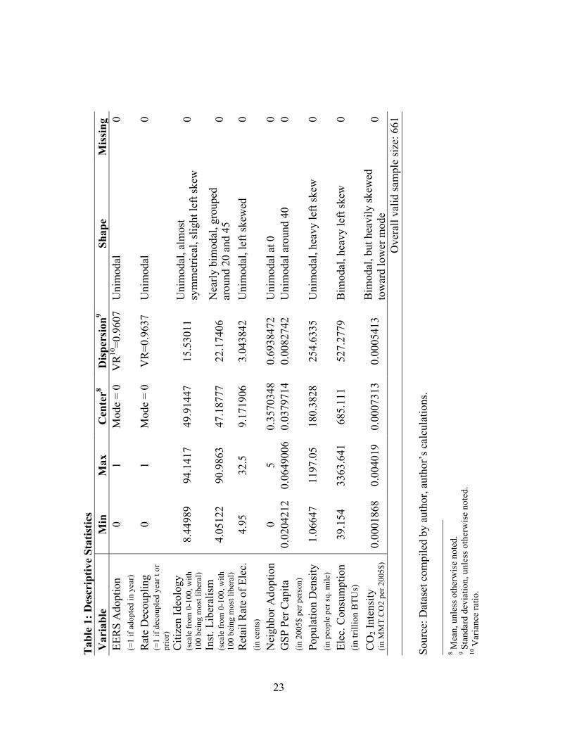
In Table 1, I provide summary statistics for each variable included in my model.

Tab

le 1

: Des

crip

tive

Stat

istic

s V

aria

ble

Min

M

ax

Cen

ter8

Dis

pers

ion9

Shap

e M

issi

ng

EER

S A

dopt

ion

0 1

Mod

e =

0 V

R10

=0.9

607

Uni

mod

al

0 (=

1 if

adop

ted

in y

ear)

R

ate

Dec

oupl

ing

0 1

Mod

e =

0 V

R=0

.963

7 U

nim

odal

0

(=1

if de

coup

led

year

t or

pr

ior)

Citi

zen

Ideo

logy

(s

cale

from

0-1

00, w

ith

100

bein

g m

ost l

iber

al)

8.44

989

94.1

417

49.9

1447

15

.530

11

Uni

mod

al, a

lmos

t sy

mm

etric

al, s

light

left

skew

0

Inst

. Lib

eral

ism

(s

cale

from

0-1

00, w

ith

100

bein

g m

ost l

iber

al)

4.05

122

90.9

863

47.1

8777

22

.174

06

Nea

rly b

imod

al, g

roup

ed

arou

nd 2

0 an

d 45

0

Ret

ail R

ate

of E

lec.

4.

95

32.5

9.

1719

06

3.04

3842

U

nim

odal

, lef

t ske

wed

0

(in c

ents

)

N

eigh

bor A

dopt

ion

0 5

0.35

7034

8 0.

6938

472

Uni

mod

al a

t 0

0 G

SP P

er C

apita

0.

0204

212

0.06

4900

6 0.

0379

714

0.00

8274

2 U

nim

odal

aro

und

40

0 (in

200

5$ p

er p

erso

n)

Popu

latio

n D

ensi

ty

1.06

647

1197

.05

180.

3828

25

4.63

35

Uni

mod

al, h

eavy

left

skew

0

(in p

eopl

e pe

r sq.

mile

)

El

ec. C

onsu

mpt

ion

39.1

54

3363

.641

68

5.11

1 52

7.27

79

Bim

odal

, hea

vy le

ft sk

ew

0 (in

trill

ion

BTU

s)

CO

2 Int

ensi

ty

(in M

MT

CO

2 pe

r 200

5$)

0.00

0186

8 0.

0040

19

0.00

0731

3 0.

0005

413

Bim

odal

, but

hea

vily

skew

ed

tow

ard

low

er m

ode

0

Ove

rall

valid

sam

ple

size

: 661

So

urce

: Dat

aset

com

pile

d by

aut

hor,

auth

or’s

cal

cula

tions

.

8 Mea

n, u

nles

s oth

erw

ise

note

d.

9 Sta

ndar

d de

viat

ion,

unl

ess o

ther

wis

e no

ted.

10

Var

ianc

e ra

tio.

23

24

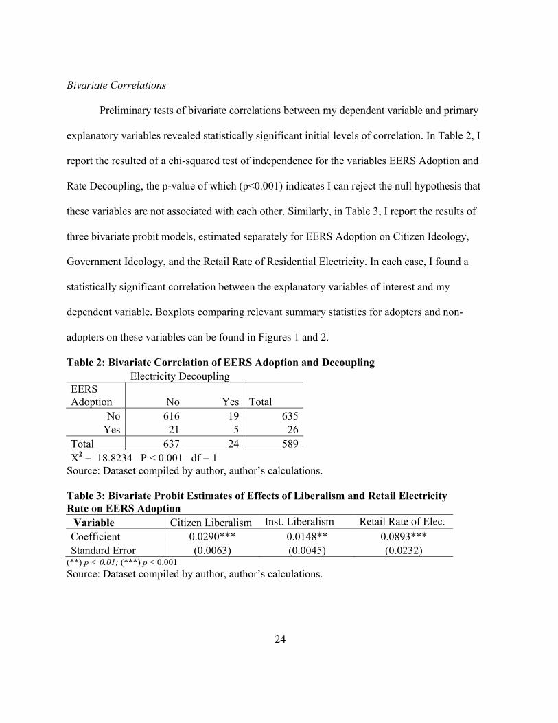
Bivariate Correlations

Preliminary tests of bivariate correlations between my dependent variable and primary

explanatory variables revealed statistically significant initial levels of correlation. In Table 2, I

report the resulted of a chi-squared test of independence for the variables EERS Adoption and

Rate Decoupling, the p-value of which (p<0.001) indicates I can reject the null hypothesis that

these variables are not associated with each other. Similarly, in Table 3, I report the results of

three bivariate probit models, estimated separately for EERS Adoption on Citizen Ideology,

Government Ideology, and the Retail Rate of Residential Electricity. In each case, I found a

statistically significant correlation between the explanatory variables of interest and my

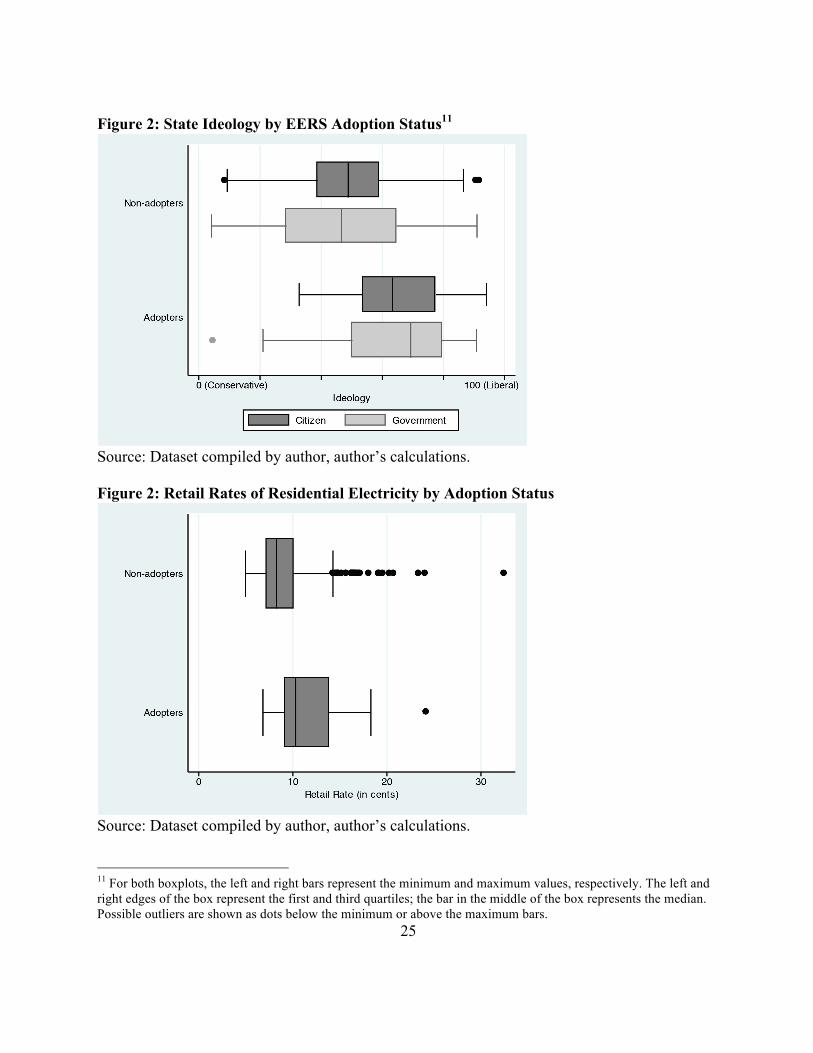
dependent variable. Boxplots comparing relevant summary statistics for adopters and non-

adopters on these variables can be found in Figures 1 and 2.

Table 2: Bivariate Correlation of EERS Adoption and Decoupling

Electricity Decoupling

EERS Adoption No Yes Total

No 616 19 635 Yes 21 5 26

Total 637 24 589 Χ2 = 18.8234 P < 0.001 df = 1  

Source: Dataset compiled by author, author’s calculations.

Table 3: Bivariate Probit Estimates of Effects of Liberalism and Retail Electricity Rate on EERS Adoption Variable Citizen Liberalism Inst. Liberalism Retail Rate of Elec. Coefficient 0.0290*** 0.0148** 0.0893*** Standard Error (0.0063) (0.0045) (0.0232)

(**) p < 0.01; (***) p < 0.001 Source: Dataset compiled by author, author’s calculations.

25

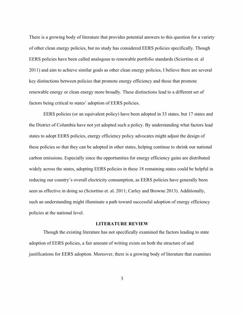
Figure 2: State Ideology by EERS Adoption Status11

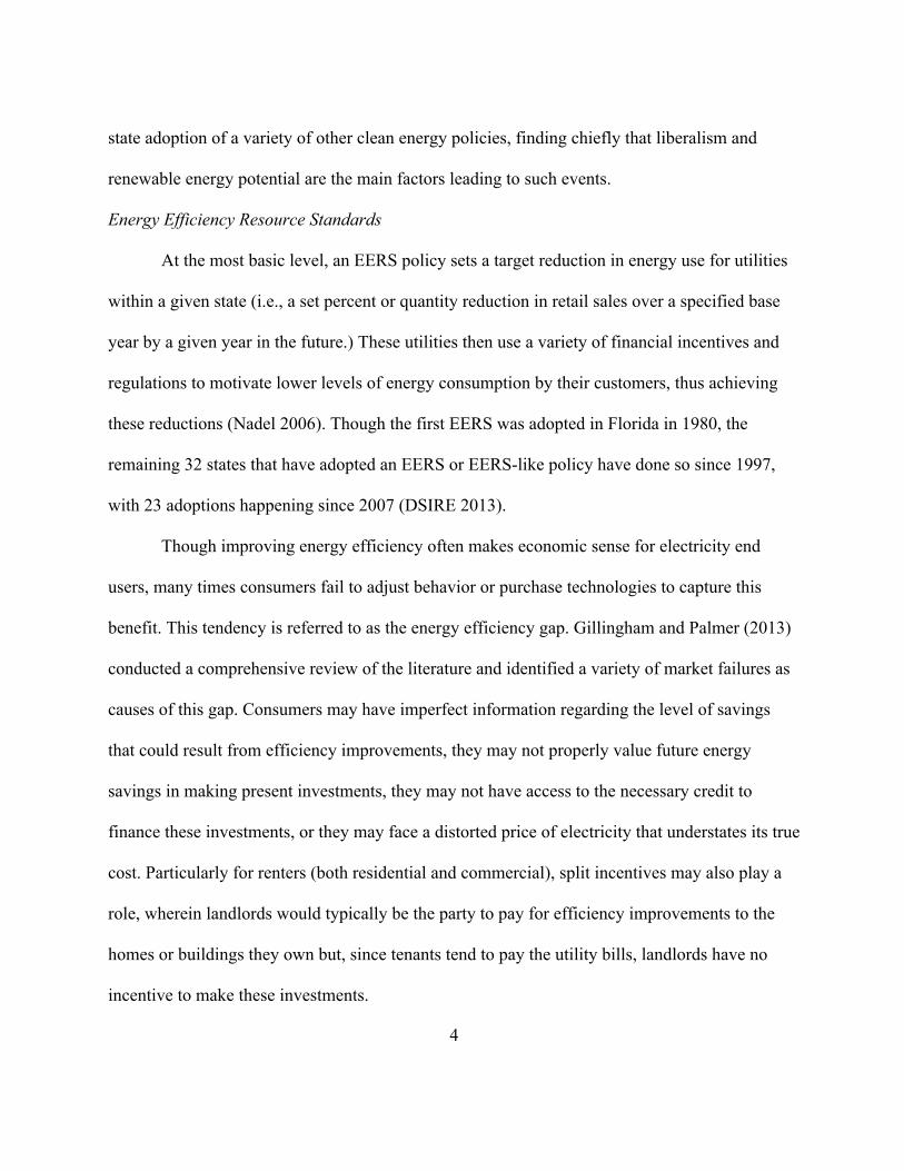
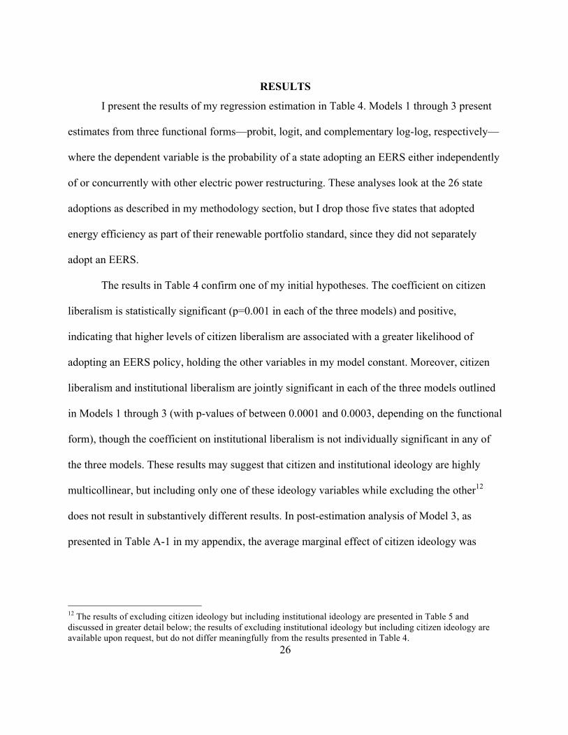
Source: Dataset compiled by author, author’s calculations. Figure 2: Retail Rates of Residential Electricity by Adoption Status

Source: Dataset compiled by author, author’s calculations.

11 For both boxplots, the left and right bars represent the minimum and maximum values, respectively. The left and right edges of the box represent the first and third quartiles; the bar in the middle of the box represents the median. Possible outliers are shown as dots below the minimum or above the maximum bars.

26

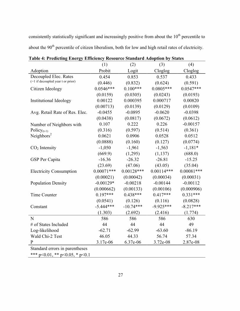
RESULTS

I present the results of my regression estimation in Table 4. Models 1 through 3 present

estimates from three functional forms—probit, logit, and complementary log-log, respectively—

where the dependent variable is the probability of a state adopting an EERS either independently

of or concurrently with other electric power restructuring. These analyses look at the 26 state

adoptions as described in my methodology section, but I drop those five states that adopted

energy efficiency as part of their renewable portfolio standard, since they did not separately

adopt an EERS.

The results in Table 4 confirm one of my initial hypotheses. The coefficient on citizen

liberalism is statistically significant (p=0.001 in each of the three models) and positive,

indicating that higher levels of citizen liberalism are associated with a greater likelihood of

adopting an EERS policy, holding the other variables in my model constant. Moreover, citizen

liberalism and institutional liberalism are jointly significant in each of the three models outlined

in Models 1 through 3 (with p-values of between 0.0001 and 0.0003, depending on the functional

form), though the coefficient on institutional liberalism is not individually significant in any of

the three models. These results may suggest that citizen and institutional ideology are highly

multicollinear, but including only one of these ideology variables while excluding the other12

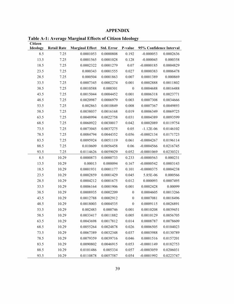
does not result in substantively different results. In post-estimation analysis of Model 3, as

presented in Table A-1 in my appendix, the average marginal effect of citizen ideology was

12 The results of excluding citizen ideology but including institutional ideology are presented in Table 5 and discussed in greater detail below; the results of excluding institutional ideology but including citizen ideology are available upon request, but do not differ meaningfully from the results presented in Table 4.

27

consistently statistically significant and increasingly positive from about the 10th percentile to

about the 90th percentile of citizen liberalism, both for low and high retail rates of electricity.

Table 4: Predicting Energy Efficiency Resource Standard Adoption by States (1) (2) (3) (4) Adoption Probit Logit Cloglog Cloglog Decoupled Elec. Rates (=1 if decoupled year t or prior)

0.454 0.853 0.537 0.433 (0.446) (0.832) (0.624) (0.591)

Citizen Ideology 0.0546*** 0.100*** 0.0805*** 0.0547***

(0.0159) (0.0305) (0.0243) (0.0193)

Institutional Ideology 0.00122 0.000395 0.000717 0.00820

(0.00713) (0.0139) (0.0129) (0.0109)

Avg. Retail Rate of Res. Elec. -0.0455 -0.0895 -0.0620 -0.0398

(0.0438) (0.0817) (0.0672) (0.0612)

Number of Neighbors with Policy(t-1)

0.107 0.222 0.226 -0.00157 (0.316) (0.597) (0.514) (0.361)

Neighbors2 0.0621 0.0906 0.0528 0.0512

(0.0888) (0.160) (0.127) (0.0774)

CO2 Intensity -1,050 -1,961 -1,563 -1,181*

(669.9) (1,295) (1,137) (688.0)

GSP Per Capita -16.36 -26.32 -26.81 -15.25

(23.69) (47.06) (43.05) (35.04)

Electricity Consumption 0.00071*** 0.00128*** 0.00114*** 0.00081***

(0.00021) (0.00042) (0.00034) (0.00031)

Population Density -0.00129* -0.00218 -0.00144 -0.00112

(0.000662) (0.00133) (0.00106) (0.000906)

Time Counter 0.197*** 0.438*** 0.417*** 0.331***

(0.0541) (0.126) (0.116) (0.0828)

Constant -5.444*** -10.74*** -9.925*** -8.217***

(1.303) (2.692) (2.416) (1.774)

N 586 586 586 630 # of States Included 44 44 44 49 Log-likelihood -62.71 -62.99 -63.60 -86.19 Wald Chi-2 Test 46.05 44.33 56.74 57.34 P 3.17e-06 6.37e-06 3.72e-08 2.87e-08 Standard errors in parentheses

*** p<0.01, ** p<0.05, * p<0.1

28

The results presented in Table 4 do not support either of my other hypotheses, that

electric rate decoupling and average retail rate of residential electricity are associated with

increased likelihood of EERS adoptions, as neither coefficient on those two variables approaches

traditional levels of statistical significance. Further, post-estimation tests reveal no set of

covariate values that yield statistically significant average marginal effects for either of these

variables.13 I return to this fact below.

Among the control variables included in the model, only electricity consumption (in all

three models) and population density (in the probit specification) are statistically significant,

holding the other variables in the model constant. The coefficients on electricity consumption are

signed as I expected (the more electricity a customer consumes, the more they spend on their

power bills, all else equal, and, therefore, the more incentive they have to support adoption of an

EERS as a means of reducing those bills) but their magnitudes are all very small. Post-estimation

tests reveal positive and statistically significant average marginal effects of electricity

consumption on adoption across the entire range of electricity consumption values. These post-

estimation findings hold for both decoupled and non-decoupled states as well as at most levels of

citizen ideology (though not for states with ideology scores in the bottom 10 percent).14

Interestingly, though previous literature (see e.g., Yi and Feicok 2012) has used population

density as a proxy for levels of air pollution, the coefficients in the probit model in Table 4 run

contrary to expectations. If people who live in areas of greater population density and, thus,

greater air pollution, want to reduce pollution through the adoption of clean energy policies like

an EERS, the expected sign on this variable would be positive; as estimated in Table 4, the point 13 These results are available upon request. 14 These post-estimation results are also available upon request.

29

estimate is actually negative, all else equal (though only significant at the 0.1 level.) The

coefficient estimates on a state’s carbon intensity approach statistical significance (with p-values

ranging from 0.117 to 0.169, depending on the functional form) and are signed as expected. No

other control variable approaches statistical significance.

Two notable observations emerge from the event history analysis approach as well. First,

the partial effects of the number of neighbors who have previously adopted and the number of

neighbors squared are not individually statistically significant, nor are they jointly significant in

any of the functional forms (with p-values ranging from 0.13 in the probit specification to 0.2382

in the cloglog specification).

Second, the coefficient estimate on the time counter variable is highly statistically

significant (p<0.001 in each of the functional forms) and positive, indicating a state is more

likely to adopt an EERS policy later in the observed time period, all else equal. As outlined in

Table A-2 in my appendix, post-estimation tests confirm this finding for states that have not

decoupled their electricity rates, showing positive and statistically significant average marginal

effects of proceeding another year in the time counter beginning in year 4, but are do not confirm

this finding for decoupled states. Moreover, I also find statistically significant positive average

marginal effects of proceeding another year in the time counter beginning in years 5 or 6 for

most levels of citizen ideology (i.e., at the median, 75th and 90th percentiles), but do not find a

statistically significant average marginal effect at lower (less liberal) citizen ideologies, as

outlined in Table A-3 in my appendix.

In my methodology section I outlined the theoretical reasoning for why states that adopt

energy efficiency measures as part of an RPS should not be considered EERS adopters for the

30

purposes of this study. In order to test the validity of this assumption, I reestimated my model

considering RPS states as EERS adopters; I present the results of this estimation in Model 4 of

Table 4, using the cloglog functional form (which, as discussed above, is best suited for rare

events like EERS adoption.) There are few meaningful differences between the two models.

Citizen ideology is still the only main explanatory variable that is statistically significant, though

its magnitude decreases from 0.0805 to 0.0547. State carbon intensity, which approached

statistical significance in the original model (p=0.169) is statistically significant (p=0.086) in the

model that includes RPS adopters, though the sign remains the same. The time counter remains

highly statistically significant in this second estimation. Otherwise, individual coefficient

estimates and levels of significance are quite similar. Both models have similar Wald statistics,

but the log-likelihood in the second model is somewhat worse. Based on these results, it appears

that states that adopt efficiency standards through their RPS may differ, but only slightly.15

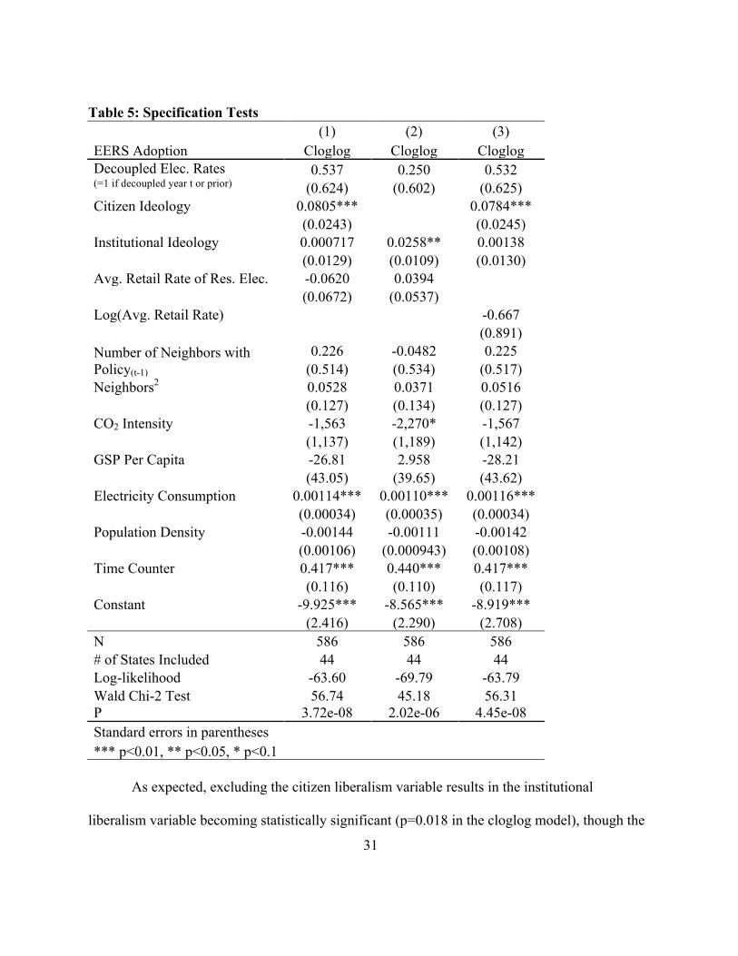
As discussed above, only one of my primary explanatory variables is statistically

significant. In Table 5, I present several specification checks that I estimated to further

investigate this result. Column 1 repeats my main model in the cloglog specification (Column 3

from Table 4). I believe that institutional liberalism is not statistically significant because a large

portion of that effect is already captured in the citizen liberalism term; the two variables are

highly correlated (correlation coefficient=0.5059). To test this explanation, I reran the model

excluding citizen liberalism as a variable. I present the results of this test in Column 2 of Table 5.

15 I similarly test my model excluding those states I have labeled as “concurrent” adopters—states who adopted an EERS at the same time as other electric sector restructuring. The results are similar to the results of my main model outlined in Columns 1 through 3 of Table 4, except that the coefficient estimates on electrical consumption are less statistically significant; citizen liberalism and the time counter variable remain significant. The results of this estimation are available upon request.

31

Table 5: Specification Tests (1) (2) (3) EERS Adoption Cloglog Cloglog Cloglog Decoupled Elec. Rates (=1 if decoupled year t or prior)

0.537 0.250 0.532 (0.624) (0.602) (0.625)

Citizen Ideology 0.0805***

0.0784***

(0.0243)

(0.0245)

Institutional Ideology 0.000717 0.0258** 0.00138

(0.0129) (0.0109) (0.0130)

Avg. Retail Rate of Res. Elec. -0.0620 0.0394

(0.0672) (0.0537)

Log(Avg. Retail Rate)

-0.667

(0.891)

Number of Neighbors with Policy(t-1)

0.226 -0.0482 0.225 (0.514) (0.534) (0.517)

Neighbors2 0.0528 0.0371 0.0516

(0.127) (0.134) (0.127)

CO2 Intensity -1,563 -2,270* -1,567

(1,137) (1,189) (1,142)

GSP Per Capita -26.81 2.958 -28.21

(43.05) (39.65) (43.62)

Electricity Consumption 0.00114*** 0.00110*** 0.00116***

(0.00034) (0.00035) (0.00034)

Population Density -0.00144 -0.00111 -0.00142

(0.00106) (0.000943) (0.00108)

Time Counter 0.417*** 0.440*** 0.417***

(0.116) (0.110) (0.117)

Constant -9.925*** -8.565*** -8.919***

(2.416) (2.290) (2.708)

N 586 586 586 # of States Included 44 44 44 Log-likelihood -63.60 -69.79 -63.79 Wald Chi-2 Test 56.74 45.18 56.31 P 3.72e-08 2.02e-06 4.45e-08 Standard errors in parentheses *** p<0.01, ** p<0.05, * p<0.1  

As expected, excluding the citizen liberalism variable results in the institutional

liberalism variable becoming statistically significant (p=0.018 in the cloglog model), though the

32

magnitude is smaller. Moreover, this result holds across each model and between the two main

sets of states I have specified.

I believe the absence of statistical significance for the coefficient on electric rate

decoupling may be the result of the relative low levels of variation in this variable. As outlined in

Table 2, decoupling has occurred in 24 of my state-year observations, and of these, EERS

adoption occurs in only five cases. Though my initial test of bivariate correlation revealed a

statistically significant association, the introduction of additional variables to the model seems to

have made the signal too indistinguishable from the noise.

Finally, the average annual retail rate of residential electricity also lacks statistical

significance. To test the possibility that its relationship with the dependent variable is actually

non-linear, I also estimated my model using the log of the average retail rate and present the

results in Column 3 of Table 5. Controlling for the log of the variable does not result in it

becoming statistically significant, nor does it have a meaningful impact on the other variables in

the model or the goodness-of-fit measures.16

DISCUSSION

To summarize, my findings indicate that higher levels of liberalism are correlated with an

increase in the probability that a state adopts an EERS policy, all else equal; otherwise, none of

my initial hypotheses hold. Additionally, higher levels of electricity consumption are associated

with small but statistically significant increases in the probability of EERS adoption, as is the

time counter variable, holding the other variables in my model constant.

16 I also reestimated the model using the logged form of GSP per capita, again with no meaningful difference in the point estimates or significances.

33

The relationship between liberalism and EERS policy is an interesting one, and my

results confirm findings from previous studies of a positive association between liberalism and

clean energy policy adoption. Further investigation is necessary, however, to disaggregate what

in particular it is about citizen liberalism that contributes to increased likelihood of adoption.

Several past studies suggest this relationship is at least partially motivated by high levels of

environmentalism among liberals and, therefore, seek to control for a state’s level of citizen

environmentalism. Both Yi and Feiock (2012) and Lyon and Yin (2010) include measures of

environmentalism but find no statistically significant effect; Stoutenborough and Beverlin (2008)

also include a measure of environmentalism as a covariate, find no statistically significant effect

on that variable, and continue to find statistical significance on their political ideology variable.

The variable Stoutenborough and Beverlin used to measure environmentalism is Hall and

Kerr’s green policy index, a cross-sectional measure ranking the states on environmental quality

that is based on measures of environmental health and policies the state has in place, which was

created in the early 1990s and that has not been updated since. I do not believe the static nature

of that index is truly reflective of evolving public consciousness on the environment. To test the

belief that a significant part of what is being reflected as an association between liberalism and

EERS adoption in my model can actually be explained by high levels of environmentalism

among liberals, I reestimated the models I present in Table 4, adding the aggregated League of

Conservation Voters (LCV) scores of each state’s delegation to the House of Representatives, as

operationalized in Konisky (2009). Each year, LCV rates each member of Congress on a 0 to 100

scale based on votes they took on particular bills that year; Konisky’s measure averages these

34

scores across the state delegation. The fact that these scores are issued annually provides a time-

variant way to include a proxy variable for a state citizenry’s environmentalism in my model.

In Table A-4 in my appendix, I present both models—both including and not including

the LCV scores—side-by-side in the cloglog functional form as Models 1 and 2. The LCV score

variable is not statistically significant, and the magnitudes and significances on the other

variables do not change meaningfully between the two models. Additionally, in Model 3 I

exclude the citizen and institutional ideology measures altogether; even in this case the

coefficient on the LCV score is not statistically significant at traditional levels (p=0.104). At

least in this operationalization of environmentalism, then, it does not seem to explain the

connection between ideology and policy adoption. Further research may reveal better ways to

account for citizen-level environmentalism, which could have an impact on my results. In the

meantime, the main takeaway, particularly for clean energy policy advocates, is that their efforts

are more likely to be effective in states with more liberal citizens. For national policymakers, it is

likely to be easiest to build support for federal-level clean energy policies among the more liberal

states first.

The fact that decoupling is not statistically significant in my model is also a notable

result. Though this finding could come as a result of the small sample size (as outlined above), it

is also worth considering the implications for Croucher’s (2011) assertion that decoupling may

make utilities less likely to oppose EERS policy adoption, and may even encourage them to

embrace such adoption. Perhaps utility embrace of EERS policies is not a sufficient condition to

guarantee adoption (though it may still be very nearly a necessary one). It may be that utility

embrace of EERS policies is only helpful in states where utilities wield outsized political

35

power—a useful implication for policymakers. This notion too could benefit from additional

research.

An additional finding relevant for policymakers is the fact that higher retail rates of

residential electricity do not appear to be correlated with increases in the probability of EERS

adoption.17 Though legislators and, particularly, utility regulators may have wanted to motivate

public support for EERS adoption by allowing for higher utility rates, this expectation is not

borne out in my findings. However, the fact that level of electricity consumption is highly

statistically significant and positively correlated with the probability of adopting an EERS

policy—even when controlling for the carbon intensity of the state’s economy and the state’s

ideology—suggests that adoption is somehow influenced by utility customers’ consumption.

Further work should be done to gain a better understanding of the nature of this relationship,

especially its theoretical basis. It is also worth investigating whether other factors about a state’s

electricity market, particularly whether it is a regulated versus deregulated market, what the

structure of the utility regulatory body looks like (e.g., Is the commission full time or part time?

How much staff support?), and how much utility competition there is in the state.

Also of interest is the fact that the time counter variable is highly statistically significant

in all specifications of my model, even when including a host of control variables, while the

neighbor variables remain statistically insignificant in every estimation. As discussed in my

literature review, traditional models of policy diffusion present three rationales for policies being

adopted by neighbors: neighbors learn by watching other neighbors implement policies;

17 I also ran my models using the total average retail rate of electricity across all sectors (i.e., not just residential but also commercial and industrial). The results, which are available upon request, are not meaningfully different for total retail rate as compared with using residential rate only.

36

neighbors compete with neighbors for jobs and industry, and the right clean energy policies

might be critical in this effort; or neighbors feel compelled to conform to a regional or national

standard. The typical assumption is that neighbors can more easily generalize lessons learned

from their neighbors to themselves and that states compete for jobs and industry at a regional—

instead of a national—level. My results tentatively suggest that perhaps this is no longer the case.

Maybe the growth of knowledge-sharing organizations (like the National Governor’s Association

or the American Council for an Energy-Efficiency Economy) allows states to learn from other

states farther afield. Moreover, maybe economic competition is truly happening at a national

level. One additional possibility is that Berry and Berry’s (2007) proposal that states feel

compelled to conform to a national standard is accurate. In any of these three cases, a variable of

the number of neighboring states that have adopted an EERS policy would not capture these

alternative types of non-geographic learning and the variable would be statistically insignificant

(as was the case in my estimations). The fact that the time counter variable is statistically

significant in my models suggests that some sort of learning may be occurring; future research

could explore these concepts.18

Finally, as discussed above, energy efficiency potential is more homogeneously

distributed across states than is renewable energy potential, particularly when controlling for size

of the state economy. Although there exists no universally recognized measure of energy

efficiency potential, controlling for that concept could change the results of my model.

Therefore, developing some measure of efficiency potential in a state could improve future

research. One starting point for such a measure could be the average age of buildings in a state,

18 The future analyst would do well to consult Mooney’s (2001) thoughts on this subject as a jumping-off point.

37

working under the assumption that older buildings have greater opportunities for efficiency

improvement.

CONCLUSION

This study sought to investigate the question of what factors lead to increases in the

likelihood that a state adopts an energy efficiency resource standard. After a review of the

literature, I hypothesized that three internal determinants—whether a state has electricity rate

decoupling, a state’s political ideology, and the average retail rate of residential electricity in a

state—would be associated with EERS adoption, all else equal. To test these hypotheses, I

estimated several multiple regression models, using the state policy adoption approach originally

proposed by Berry and Berry (1990) to determine the effects of these explanatory variables and

other control variables on a state’s adoption likelihood.

Chiefly, my findings confirm the conclusion that emerges from the extant clean energy

policy adoption literature: a state’s political liberalness, particularly that of its citizens, is one of

the critical factors that increases the probability of policy adoption. I failed to find significant

effects on my other two explanatory variables (though for decoupling I strongly suspect this

result is due, at least partially, to the lack of states who have adopted such policies). Among my

control variables, the effect of electricity consumption was consistently positive and statistically

significant, holding other factors equal, suggesting that something about greater electricity use

(even while controlling for the price of electricity) motivates adoption of EERS policies. I failed

to find evidence that states whose neighbors had adopted an EERS policy were themselves more

likely to adopt, but the significance of the coefficient on the time counter variable suggests some

form of policy diffusion process may still take place. My study also suggests several avenues for

38

future research, including a deeper understanding of why liberalism is associated with increases

in probability for adoption, further refining electricity market factors that may be associated with

the increasing likelihood of adoption, and continued research into the effect of rate decoupling.

39

APPENDIX

Table A-1: Average Marginal Effects of Citizen Ideology Citizen Ideology Retail Rate Marginal Effect Std. Error P-value 95% Confidence Interval

8.5 7.25 0.0001053 0.0000808 0.192 -0.000053 0.0002636 13.5 7.25 0.0001565 0.0001028 0.128 -0.000045 0.000358 18.5 7.25 0.0002322 0.0001279 0.07 -0.0000185 0.0004829 23.5 7.25 0.000343 0.0001555 0.027 0.0000383 0.0006478 28.5 7.25 0.000504 0.0001863 0.007 0.0001389 0.000869 33.5 7.25 0.0007345 0.0002274 0.001 0.0002888 0.0011802 38.5 7.25 0.0010588 0.000301 0 0.0004688 0.0016488 43.5 7.25 0.0015044 0.0004452 0.001 0.0006318 0.0023771 48.5 7.25 0.0020987 0.0006979 0.003 0.0007308 0.0034666 53.5 7.25 0.002863 0.0010849 0.008 0.0007367 0.0049893 58.5 7.25 0.0038037 0.0016168 0.019 0.0006349 0.0069725 63.5 7.25 0.0048994 0.0022758 0.031 0.0004389 0.0093599 68.5 7.25 0.0060922 0.0030017 0.042 0.0002089 0.0119754 73.5 7.25 0.0073045 0.0037275 0.05 -1.12E-06 0.0146102 78.5 7.25 0.0084794 0.0044352 0.056 -0.0002134 0.0171723 83.5 7.25 0.0095924 0.0051119 0.061 -0.0004267 0.0196114 88.5 7.25 0.010609 0.0056458 0.06 -0.0004566 0.0216745 93.5 7.25 0.0114626 0.0059029 0.052 -0.0001069 0.0230321

8.5 10.29 0.0000873 0.0000733 0.233 -0.0000563 0.000231 13.5 10.29 0.00013 0.000094 0.167 -0.0000542 0.0003143 18.5 10.29 0.0001931 0.0001177 0.101 -0.0000375 0.0004238 23.5 10.29 0.0002859 0.0001429 0.045 5.85E-06 0.000566 28.5 10.29 0.0004212 0.0001675 0.012 0.000093 0.0007495 33.5 10.29 0.0006164 0.0001906 0.001 0.0002428 0.00099 38.5 10.29 0.0008935 0.0002209 0 0.0004605 0.0013266 43.5 10.29 0.0012788 0.0002912 0 0.0007081 0.0018496 48.5 10.29 0.0018003 0.0004535 0 0.0009115 0.0026891 53.5 10.29 0.002483 0.000746 0.001 0.0010208 0.0039451 58.5 10.29 0.0033417 0.0011882 0.005 0.0010129 0.0056705 63.5 10.29 0.0043698 0.0017812 0.014 0.0008787 0.0078609 68.5 10.29 0.0055264 0.0024878 0.026 0.0006505 0.0104023 73.5 10.29 0.0067389 0.0032348 0.037 0.0003988 0.0130789 78.5 10.29 0.0079359 0.0039716 0.046 0.0001516 0.0157201 83.5 10.29 0.0090802 0.0046915 0.053 -0.0001149 0.0182753 88.5 10.29 0.0101486 0.005334 0.057 -0.0003059 0.0206031 93.5 10.29 0.0110878 0.0057587 0.054 -0.0001992 0.0223747

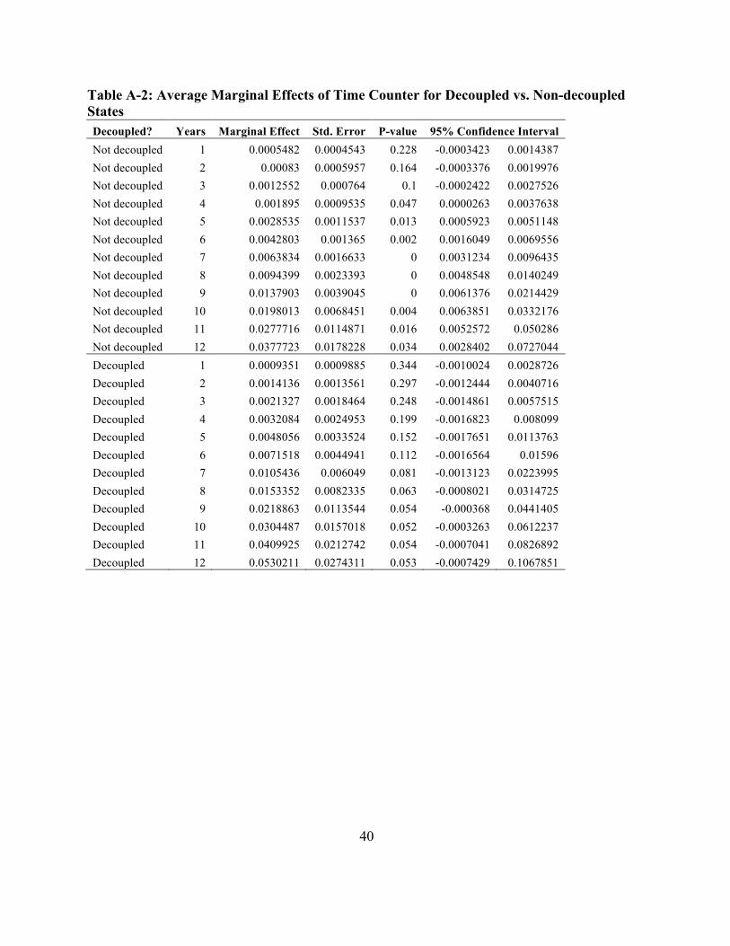
40

Table A-2: Average Marginal Effects of Time Counter for Decoupled vs. Non-decoupled States Decoupled? Years Marginal Effect Std. Error P-value 95% Confidence Interval Not decoupled 1 0.0005482 0.0004543 0.228 -0.0003423 0.0014387 Not decoupled 2 0.00083 0.0005957 0.164 -0.0003376 0.0019976 Not decoupled 3 0.0012552 0.000764 0.1 -0.0002422 0.0027526 Not decoupled 4 0.001895 0.0009535 0.047 0.0000263 0.0037638 Not decoupled 5 0.0028535 0.0011537 0.013 0.0005923 0.0051148 Not decoupled 6 0.0042803 0.001365 0.002 0.0016049 0.0069556 Not decoupled 7 0.0063834 0.0016633 0 0.0031234 0.0096435 Not decoupled 8 0.0094399 0.0023393 0 0.0048548 0.0140249 Not decoupled 9 0.0137903 0.0039045 0 0.0061376 0.0214429 Not decoupled 10 0.0198013 0.0068451 0.004 0.0063851 0.0332176 Not decoupled 11 0.0277716 0.0114871 0.016 0.0052572 0.050286 Not decoupled 12 0.0377723 0.0178228 0.034 0.0028402 0.0727044 Decoupled 1 0.0009351 0.0009885 0.344 -0.0010024 0.0028726 Decoupled 2 0.0014136 0.0013561 0.297 -0.0012444 0.0040716 Decoupled 3 0.0021327 0.0018464 0.248 -0.0014861 0.0057515 Decoupled 4 0.0032084 0.0024953 0.199 -0.0016823 0.008099 Decoupled 5 0.0048056 0.0033524 0.152 -0.0017651 0.0113763 Decoupled 6 0.0071518 0.0044941 0.112 -0.0016564 0.01596 Decoupled 7 0.0105436 0.006049 0.081 -0.0013123 0.0223995 Decoupled 8 0.0153352 0.0082335 0.063 -0.0008021 0.0314725 Decoupled 9 0.0218863 0.0113544 0.054 -0.000368 0.0441405 Decoupled 10 0.0304487 0.0157018 0.052 -0.0003263 0.0612237 Decoupled 11 0.0409925 0.0212742 0.054 -0.0007041 0.0826892 Decoupled 12 0.0530211 0.0274311 0.053 -0.0007429 0.1067851

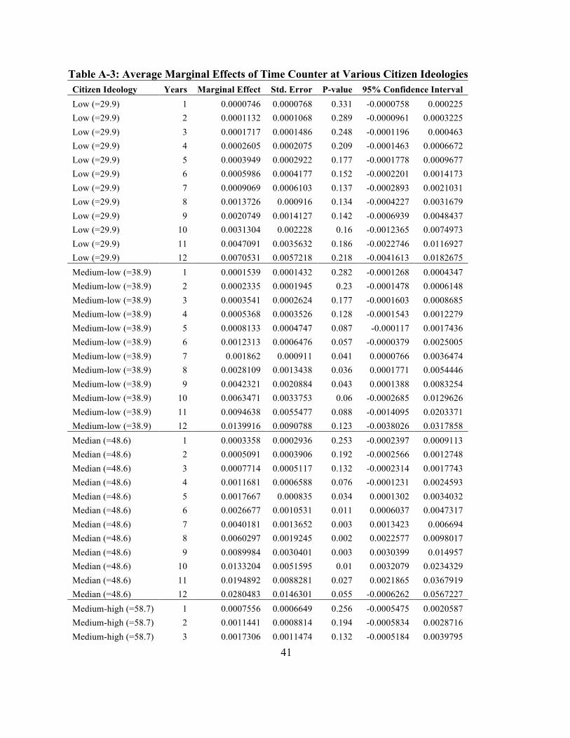
41

Table A-3: Average Marginal Effects of Time Counter at Various Citizen Ideologies Citizen Ideology Years Marginal Effect Std. Error P-value 95% Confidence Interval Low (=29.9) 1 0.0000746 0.0000768 0.331 -0.0000758 0.000225 Low (=29.9) 2 0.0001132 0.0001068 0.289 -0.0000961 0.0003225 Low (=29.9) 3 0.0001717 0.0001486 0.248 -0.0001196 0.000463 Low (=29.9) 4 0.0002605 0.0002075 0.209 -0.0001463 0.0006672 Low (=29.9) 5 0.0003949 0.0002922 0.177 -0.0001778 0.0009677 Low (=29.9) 6 0.0005986 0.0004177 0.152 -0.0002201 0.0014173 Low (=29.9) 7 0.0009069 0.0006103 0.137 -0.0002893 0.0021031 Low (=29.9) 8 0.0013726 0.000916 0.134 -0.0004227 0.0031679 Low (=29.9) 9 0.0020749 0.0014127 0.142 -0.0006939 0.0048437 Low (=29.9) 10 0.0031304 0.002228 0.16 -0.0012365 0.0074973 Low (=29.9) 11 0.0047091 0.0035632 0.186 -0.0022746 0.0116927 Low (=29.9) 12 0.0070531 0.0057218 0.218 -0.0041613 0.0182675 Medium-low (=38.9) 1 0.0001539 0.0001432 0.282 -0.0001268 0.0004347 Medium-low (=38.9) 2 0.0002335 0.0001945 0.23 -0.0001478 0.0006148 Medium-low (=38.9) 3 0.0003541 0.0002624 0.177 -0.0001603 0.0008685 Medium-low (=38.9) 4 0.0005368 0.0003526 0.128 -0.0001543 0.0012279 Medium-low (=38.9) 5 0.0008133 0.0004747 0.087 -0.000117 0.0017436 Medium-low (=38.9) 6 0.0012313 0.0006476 0.057 -0.0000379 0.0025005 Medium-low (=38.9) 7 0.001862 0.000911 0.041 0.0000766 0.0036474 Medium-low (=38.9) 8 0.0028109 0.0013438 0.036 0.0001771 0.0054446 Medium-low (=38.9) 9 0.0042321 0.0020884 0.043 0.0001388 0.0083254 Medium-low (=38.9) 10 0.0063471 0.0033753 0.06 -0.0002685 0.0129626 Medium-low (=38.9) 11 0.0094638 0.0055477 0.088 -0.0014095 0.0203371 Medium-low (=38.9) 12 0.0139916 0.0090788 0.123 -0.0038026 0.0317858 Median (=48.6) 1 0.0003358 0.0002936 0.253 -0.0002397 0.0009113 Median (=48.6) 2 0.0005091 0.0003906 0.192 -0.0002566 0.0012748 Median (=48.6) 3 0.0007714 0.0005117 0.132 -0.0002314 0.0017743 Median (=48.6) 4 0.0011681 0.0006588 0.076 -0.0001231 0.0024593 Median (=48.6) 5 0.0017667 0.000835 0.034 0.0001302 0.0034032 Median (=48.6) 6 0.0026677 0.0010531 0.011 0.0006037 0.0047317 Median (=48.6) 7 0.0040181 0.0013652 0.003 0.0013423 0.006694 Median (=48.6) 8 0.0060297 0.0019245 0.002 0.0022577 0.0098017 Median (=48.6) 9 0.0089984 0.0030401 0.003 0.0030399 0.014957 Median (=48.6) 10 0.0133204 0.0051595 0.01 0.0032079 0.0234329 Median (=48.6) 11 0.0194892 0.0088281 0.027 0.0021865 0.0367919 Median (=48.6) 12 0.0280483 0.0146301 0.055 -0.0006262 0.0567227 Medium-high (=58.7) 1 0.0007556 0.0006649 0.256 -0.0005475 0.0020587 Medium-high (=58.7) 2 0.0011441 0.0008814 0.194 -0.0005834 0.0028716 Medium-high (=58.7) 3 0.0017306 0.0011474 0.132 -0.0005184 0.0039795

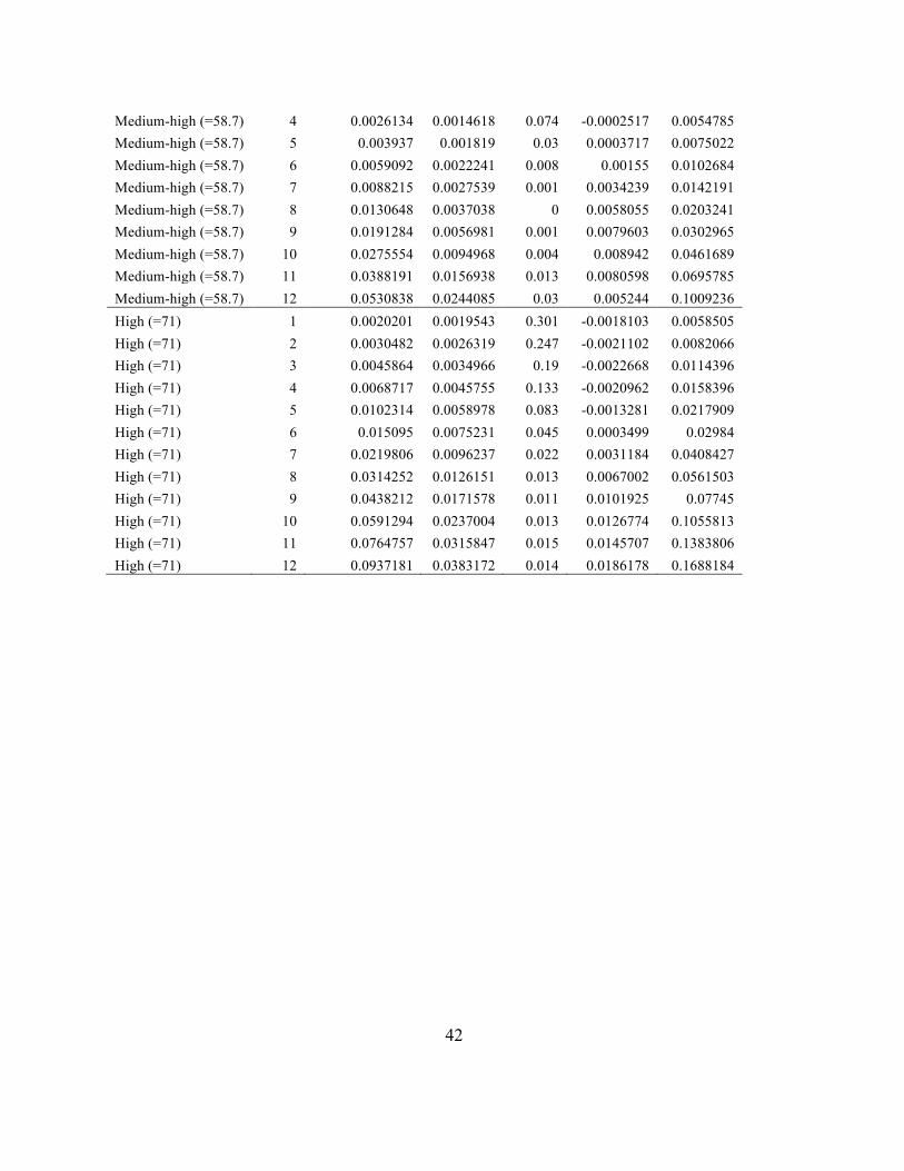
42

Medium-high (=58.7) 4 0.0026134 0.0014618 0.074 -0.0002517 0.0054785 Medium-high (=58.7) 5 0.003937 0.001819 0.03 0.0003717 0.0075022 Medium-high (=58.7) 6 0.0059092 0.0022241 0.008 0.00155 0.0102684 Medium-high (=58.7) 7 0.0088215 0.0027539 0.001 0.0034239 0.0142191 Medium-high (=58.7) 8 0.0130648 0.0037038 0 0.0058055 0.0203241 Medium-high (=58.7) 9 0.0191284 0.0056981 0.001 0.0079603 0.0302965 Medium-high (=58.7) 10 0.0275554 0.0094968 0.004 0.008942 0.0461689 Medium-high (=58.7) 11 0.0388191 0.0156938 0.013 0.0080598 0.0695785 Medium-high (=58.7) 12 0.0530838 0.0244085 0.03 0.005244 0.1009236 High (=71) 1 0.0020201 0.0019543 0.301 -0.0018103 0.0058505 High (=71) 2 0.0030482 0.0026319 0.247 -0.0021102 0.0082066 High (=71) 3 0.0045864 0.0034966 0.19 -0.0022668 0.0114396 High (=71) 4 0.0068717 0.0045755 0.133 -0.0020962 0.0158396 High (=71) 5 0.0102314 0.0058978 0.083 -0.0013281 0.0217909 High (=71) 6 0.015095 0.0075231 0.045 0.0003499 0.02984 High (=71) 7 0.0219806 0.0096237 0.022 0.0031184 0.0408427 High (=71) 8 0.0314252 0.0126151 0.013 0.0067002 0.0561503 High (=71) 9 0.0438212 0.0171578 0.011 0.0101925 0.07745 High (=71) 10 0.0591294 0.0237004 0.013 0.0126774 0.1055813 High (=71) 11 0.0764757 0.0315847 0.015 0.0145707 0.1383806 High (=71) 12 0.0937181 0.0383172 0.014 0.0186178 0.1688184

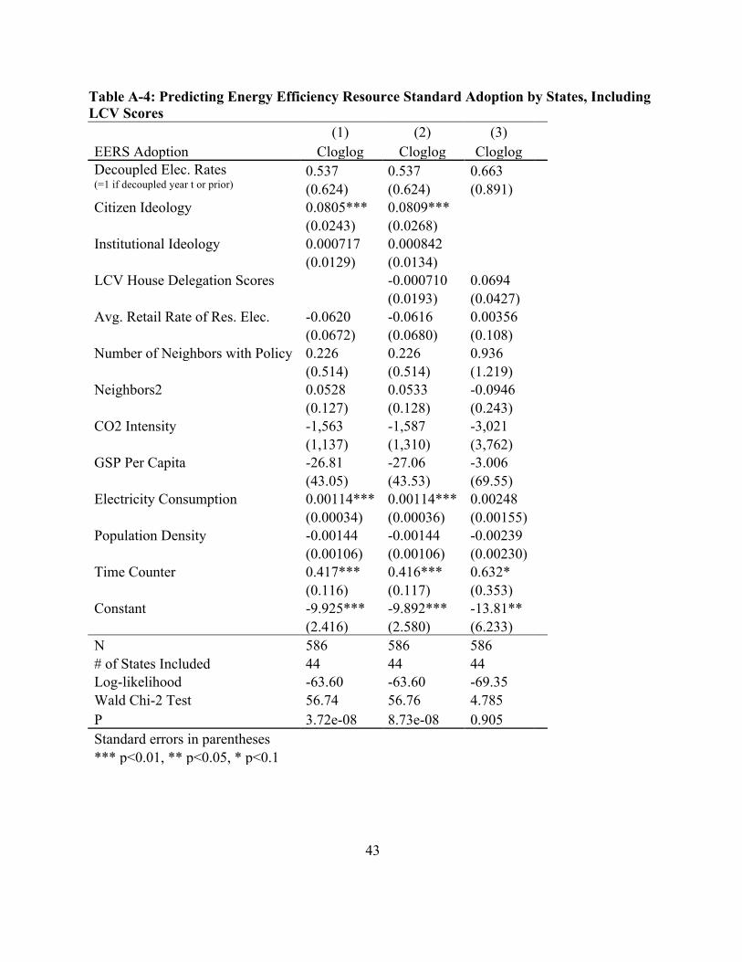
43

Table A-4: Predicting Energy Efficiency Resource Standard Adoption by States, Including LCV Scores (1) (2) (3) EERS Adoption Cloglog Cloglog Cloglog Decoupled Elec. Rates (=1 if decoupled year t or prior)

0.537 0.537 0.663 (0.624) (0.624) (0.891)

Citizen Ideology 0.0805*** 0.0809***

(0.0243) (0.0268)

Institutional Ideology 0.000717 0.000842

(0.0129) (0.0134)

LCV House Delegation Scores

-0.000710 0.0694

(0.0193) (0.0427)

Avg. Retail Rate of Res. Elec. -0.0620 -0.0616 0.00356

(0.0672) (0.0680) (0.108)

Number of Neighbors with Policy 0.226 0.226 0.936

(0.514) (0.514) (1.219)

Neighbors2 0.0528 0.0533 -0.0946

(0.127) (0.128) (0.243)

CO2 Intensity -1,563 -1,587 -3,021

(1,137) (1,310) (3,762)

GSP Per Capita -26.81 -27.06 -3.006

(43.05) (43.53) (69.55)

Electricity Consumption 0.00114*** 0.00114*** 0.00248

(0.00034) (0.00036) (0.00155)

Population Density -0.00144 -0.00144 -0.00239

(0.00106) (0.00106) (0.00230)

Time Counter 0.417*** 0.416*** 0.632*

(0.116) (0.117) (0.353)

Constant -9.925*** -9.892*** -13.81**

(2.416) (2.580) (6.233)

N 586 586 586 # of States Included 44 44 44 Log-likelihood -63.60 -63.60 -69.35 Wald Chi-2 Test 56.74 56.76 4.785 P 3.72e-08 8.73e-08 0.905 Standard errors in parentheses *** p<0.01, ** p<0.05, * p<0.1

44

REFERENCES

Allison, P. (1984). Event history analysis. Sage University Paper Series on Quantitative Applications in the Social Sciences, 07-46. Newbury Park, CA: Sage.

Berry, F. S., & Berry, W. D. (1990). State lottery adoptions as policy innovations: An event history analysis. The American Political Science Review, 84(2), 395-415.

Berry, F. S., & Berry, W. D. (2007). Innovation and diffusion models in policy research. In P. A. Sabatier (Ed.), Theories of the Policy Process (2nd ed., pp. 223). Boulder, CO: Westview Press.

Berry, W. D., Fording, R. C., Ringquist, E. J., Hanson, R. L., & Klarner, C. E. (2010). Measuring citizen and government ideology in the US states: A re-appraisal. State Politics & Policy Quarterly, 10(2), 117-135.

Berry, W. D., Ringquist, E. J., Fording, R. C., & Hanson, R. L. (1998). Measuring citizen and government ideology in the American states, 1960-93. American Journal of Political Science, 42(1), 327-348.

Bipartisan Policy Center. (2013). America’s energy resurgence: Sustaining success, confronting challenges.

Boehmke, F. J., & Skinner, P. (2012). State policy innovativeness revisited. State Politics & Policy Quarterly, 12(3), 303-329.

Box-Steffensmeier, J. M., & Jones, B. S. (2004). Event History Modeling: A Guide for Social Scientists Cambridge University Press.

Brennan, T. J., & Palmer, K. L. (2013). Energy efficiency resource standards: Economics and policy. Utilities Policy, 25, 58-68.

Buckley, J., & Westerland, C. (2004). Duration dependence, functional form, and corrected standard errors: Improving EHA models of state policy diffusion. State Politics & Policy Quarterly, 4(1), 94-113.

Carley, S. (2011). The era of state energy policy innovation: A review of policy instruments. Review of Policy Research, 28(3), 265-294.

Carley, S., & Browne, T. R. (2013). Innovative US energy policy: A review of states' policy experiences. Wiley Interdisciplinary Reviews: Energy and Environment, 2(5), 488-506.

45

Carley, S., & Miller, C. J. (2012). Regulatory stringency and policy drivers: A reassessment of renewable portfolio standards. Policy Studies Journal, 40(4), 730-756.

Chandler, J. (2009). Trendy solutions: Why do states adopt sustainable energy portfolio standards? Energy Policy, 37(8), 3274-3281.

Croucher, M. (2011). Are energy efficiency standards within the electricity sector a form of regulatory capture? Energy Policy, 39(6), 3602-3604.

Database of State Incentives for Renewables & Efficiency (DSIRE). (2013). DSIRE: Database of state incentives for renewables & efficiency. Retrieved October 22, 2013, from www.dsireusa.org.

Energy Information Administration. (2013). Average retail price of electricity to ultimate customers: By state, by provider, annual back to 1990 (form EIA-861). Retrieved November 14, 2013, from http://www.eia.gov/electricity/data/state/avgprice_annual.xls.

Energy Information Administration. (2013). State CO2 Estimates. Retrieved November 14, 2013, from http://www.eia.gov/environment/emissions/state/state_emissions.cfm.

Fording, R. C. (2012). State ideology data. Retrieved November 14, 2013, from http://rcfording.wordpress.com/state-ideology-data.

Fowler, L., & Breen, J. (2013). The impact of political factors on states’ adoption of renewable portfolio standards. The Electricity Journal, 26(2), 79-94.

Gillingham, K., & Palmer, K. (2013). Bridging the energy efficiency gap. (No. RFF DP 13-02). Washington, DC: Resources for the Future.

Granade, H. C., Creyts, J., Derkach, A., Farese, P., Nyquist, S., & and Ostrowski, K. (2009). Unlocking energy efficiency in the U.S. economy. McKinsey & Company.

Huang, M., Alavalapati, J. R., Carter, D. R., & Langholtz, M. H. (2007). Is the choice of renewable portfolio standards random? Energy Policy, 35(11), 5571-5575.

Konisky, D. M. (2009). Assessing US state susceptibility to environmental regulatory competition. State Politics & Policy Quarterly, 9(4), 404-428.

Lyon, T. P., & Yin, H. (2010). Why do states adopt renewable portfoli standards?: An empirical investigation. The Energy Journal, 31(3), 133.

46

Matisoff, D. C. (2008). The adoption of state climate change policies and renewable portfolio standards: Regional diffusion or internal determinants? Review of Policy Research, 25(6), 527-546.

Metcalf, G. E. (2007). Federal tax policy towards energy. Tax Policy and the Economy, 21, 145-184.

Mohr, L. B. (1969). Determinants of innovation in organizations. The American Political Science Review, 63(1), 111-126.

Mooney, C. Z. (2001). Modeling regional effects on state policy diffusion. Political Research Quarterly, 54(1), 103-124.

Nadel, S. (2006). Energy efficiency resource standards: Experience and recommendations. (No. E063). American Council for an Energy-Efficient Economy.

New State Ice Co. v. Liebmann, 285 U.S. 262 (1932).

Palmer, K. L., Grausz, S., Beasley, B., & Brennan, T. J. (2013). Putting a floor on energy savings: Comparing state energy efficiency resource standards. Utilities Policy, 25, 43-57.

Sciortino, M., Nowak, S., Witte, P., York, D., & Kushler, M. (2011). Energy efficiency resource standards: A progress report on state experience. (No. U112). American Council for an Energy-Efficient Economy.

Stoutenborough, J. W., & Beverlin, M. (2008). Encouraging Pollution‐Free energy: The diffusion of state net metering policies. Social Science Quarterly, 89(5), 1230-1251.

Sullivan, D., Wang, D., & Bennett, D. (2011). Essential to energy efficiency, but easy to explain: Frequently asked questions about decoupling. The Electricity Journal, 24(8), 56-70.

UCLA: Statistical Consulting Group. (2014). Statistical computing seminars: Survival analysis with STATA. Retrieved April 2, 2014, from http://www.ats.ucla.edu/stat/stata/seminars/stata_survival/.

U.S. Census Bureau. (2012). Intercensal estimates. Retrieved November 14, 2013, from http://www.census.gov/popest/data/intercensal/index.html.

U.S. Census Bureau. (n.d.). State and county QuickFacts. Retrieved November 14, 2013, from http://quickfacts.census.gov/qfd/download_data.html.

47

U.S. Department of Commerce Bureau of Economic Analysis. (n.d.). Regional data: GDP and personal income. Retrieved November 14, 2013, from http://www.bea.gov/iTable/index_regional.cfm.

Walker, J. L. (1969). The diffusion of innovations among the American states. The American Political Science Review, 63(3), 880-899.

Yi, H., & Feiock, R. C. (2012). Policy tool interactions and the adoption of state renewable portfolio standards. Review of Policy Research, 29(2), 193-206.

York, D., Kushler, M., Hayes, S., Sienkowski, S., Bell, C., & Kihm, S. (2013). Making the business case for energy efficiency: Case studies of supportive utility regulation. (No. U133). American Council for an Energy-Efficient Economy.