Predicting the stiffness and strength of human femurs with realmetastatic tumors

Zohar Yosibasha,∗, Romina Plitman Mayoa, Gal Dahana, Nir Trabelsib, Gail Amirc, CharlesMilgromd

aDepartment of Mechanical Engineering, Ben-Gurion University, Beer-Sheva, IsraelbDepartment of Mechanical Engineering, Shamoon College of Engineering, Beer-Sheva, Israel

cDepartment of Pathology, Hadassah University Hospital, Jerusalem, IsraeldDepartment of Orthopaedics, Hadassah University Hospital, Jerusalem, Israel

Abstract

Background: Predicting patient specific risk of fracture in femurs with metastatic tu-

mors and the need for surgical intervention are of major clinical importance. Recent patient-

specific high-order finite element methods (p-FEMs) based on CT-scans demonstrated ac-

curate results for healthy femurs, so that their application to metastatic affected femurs is

considered herein.

Methods: Radiographs of fresh frozen proximal femurs specimens from donors that died

of cancer were examined, and seven pairs with metastatic tumor identified. These were CT-

scanned, instrumented by strain-gauges and loaded in stance position at three inclination

angles. Finally the femurs were loaded until fracture that usually occurred at the neck.

Histopathology was performed to determine whether metastatic tumors are present at frac-

tured surfaces. Following each experiment p-FE models were created based on the CT-scans

mimicking the mechanical experiments. The predicted displacements, strains and yield loads

were compared to experimental observations.

Results: The predicted strains and displacements showed an excellent agreement with

the experimental observations with a linear regression slope of 0.95 and a coefficient of re-

gression R2 = 0.967. A good correlation was obtained between the predicted yield load and

the experimental observed yield, with a linear regression slope of 0.80 and a coefficient of

∗Corresponding authorEmail address: zohary@bgu.ac.il (Zohar Yosibash)

Preprint submitted to Bone September 24, 2014

regression R2 = 0.78.

Discussion: CT-based patient-specific p-FE models of femurs with real metastatic tu-

mors were demonstrated to predict the mechanical response very well. A simplified yield

criterion based on the computation of principal strains was also demonstrated to predict the

yield force in most of the cases, especially for femurs that failed at small loads. In view

of the limited capabilities to predict risk of fracture in femurs with metastatic tumors used

nowadays, the p-FE methodology validated herein may be very valuable in making clinical

decisions.Keywords: Metastatic tumors, p-FEMs, femur

1. Introduction1

One third to one half of all cancers (especially breast, prostate, renal, thyroid, and lung2

cancer) metastasize to bones [3], which in turn leads to pathologic fractures or symptoms3

severe enough to require treatment in 30-50% of these cases [9]. Currently, to assess the4

fracture risk in patient with skeletal metastasis clinicians use the Mirels’ criterion or rely5

on their past clinical experience. The Mirels’ criterion is however not very specific (91%6

sensitive, 35% specific) [18, 4] and results in unnecessary internal fixation procedures in two7

thirds of the patients.8

In recent years more accurate methods based on computed tomography (CT) have been9

suggested to predict the risk of fracture that take into consideration both the patient specific10

geometrical description and the spatial distribution of material properties in bones with11

metastases (especially lytic types). These include the CT based structural rigidly analysis12

(CTRA) that is mainly applicable to shaft regions [21, 19] and CT based finite element13

methods (FEMs) [13, 14, 22, 15, 23, 5]. A summary of past FE investigations for human14

femurs with realistic/simulated metastatic tumors is given in Table 1.15

Most past studies that use FEMs for the assessment of fractures risk in femurs with16

metastases are limited because they are “validated” by healthy bones with artificially created17

defects that do not well represent actual metastatic tumors.18

Metastases are associated with major trabecular bone loss before cortical bone loss and19

2

Reference # of femurs Kind of test

Keyak et al. [13] 12 shafts (death=cancer) 4PB

Keyak at al. [14] 44 femurs (8 with metastases) Compression

Spruijt et al. [22] 22 healthy shafts Torsion

Tanck et al. [23] 12 healthy femurs Compression

Deriks et al. [5] 20 healthy pairs Compression

Reference Defects description Comments

Keyak et al. [13] Realistic FE+Exp on femur shafts

Keyak at al. [14] Realistic FE+Exp on proximal femurs

Spruijt et al. [22] Transcortical hole subtrochanteric region FE+Exp on shafts

Tanck et al. [23] Drilled FE+Exp on proximal femurs

Deriks et al. [5] Drilled FE+Exp on proximal femurs

Table 1: Summary of past FE simulations validated by experiments on human femurs with realistic/simulated

tumors.

a considerable percentage of these tumors are mixed blastic-lytic ones. In addition, the20

borders between tumor and non-tumor affected areas usually do not have sharp boundaries.21

In this respect we cite [13], “...we found that femoral shafts with hemispheric burr holes do not22

accurately simulate the force versus displacement behavior of shafts with metastatic lesions.”23

To the best of the authors’ knowledge, the only previous study that considers FEMs of fresh24

frozen proximal femurs with real metastases that are validated by experimental observations25

is [14]. In that pioneering study eight femurs with metastatic tumors, out of 44 femurs26

altogether, are considered for the determination of the fracture load. In [14] the authors27

had to artificially alter the material properties of the bone tissue in the FE analysis on28

a “calibration cohort” of 18 femurs, 4 of which are with metastases (by comparing FEM29

fracture loads to the ones in experiments) to enable a better prediction of subsequent 2630

femurs (4 with a metastasis). In spite of the fact that fracture occurrence is based on stress31

and/or strain criteria, none of the previous publications on the topic report on any validation32

3

procedure for these quantities. Finally, none of these past publications performed histological33

analyses of the fractured bones to determine the type of metastases and whether the presence34

of a tumor influenced the fracture location.35

Leveraging the success of predicting the mechanical response of intact femurs with very36

high accuracy by high-order FEMs [27, 31, 25, 26], we extend the developed methods to37

femurs with metastatic tumors. There are four novelties in the present study: a) A large38

cohort of femurs with realistic metastatic tumors (fourteen femurs from seven donors) is39

considered; b) A variety of metastatic tumors representing several different types of cancers40

are investigated; c) A detailed and thorough investigation of the femur’s mechanical response41

(displacements and strains are validated); d) Pathological examination of the fracture surface42

to identify whether metastases are present and the precise tumor type.43

We aim to provide rigorous evidence that patient-specific high-order FEMs are accurate44

and reliable to be used as a decision support system by orthopedic surgeons, especially in45

complex situations of femurs with metastatic tumors.46

2. Materials and Methods47

Fourteen fresh-frozen human femurs (7 pairs denoted by FFM1-FFM7) with proximal48

metastatic tumors were chosen by an experienced orthopedic physician based on radiographs49

(see Figure 1) and cause of death. Donor details are summarized in Table 2. These50

femurs underwent mechanical experiments after they were defrosted, cleaned of soft tissues51

and degreased with ethanol. The proximal femur (∼ 250 mm from the top of the head)52

was fixed into a cylindrical metallic sleeve by PMMA, immersed in water and CT-scanned53

with K2HPO4 calibration phantoms. A Phillips Brilliance 64 CT axial scan without overlap54

(Einhoven, Netherlands - 120-140 kVp, 250 mAs, 0.75 - 1.5 mm slice thickness) was used with55

pixel size of 0.2-0.7 mm. Thirteen uniaxial strain gauges (SGs) (Vishay CEA-06-062UR-350)56

were bonded to the surface of each femur at the typical locations shown in Figure 2. Details57

on the procedure are available in [31].58

4

Donor Label Age (Years) Height [m] Weight [Kg] Gender Cause of Death

FFM1 77 1.80 50 Male Lung Cancer

FFM2 74 1.50 45 Female Colon Cancer

FFM3 55 1.75 73 Male Pancreatic Cancer

FFM4 79 1.62 55 Female Breast Cancer

FFM5 76 1.60 50 Female Renal Cell Cancer

FFM6 71 1.90 84 Male Prostate Cancer

FFM7 75 1.62 41 Female Cervical Cancer

Table 2: Donor details.

2.1. In-vitro experiments59

Mechanical experiments were conducted on each pair (right and left femurs) on the day60

of defrosting in a configuration that mimics a simple stance position (see Figure 3). The61

femurs were loaded through their head by a flat plate (on a 1-cm diameter circular surface)62

and clamped at the distal part. Loading was applied at three different inclination angles63

(0◦, 7◦ and 15◦), see Figure 3. Most of the experiments were performed with a Shimadzu64

AG-IC machine (Shimadzu Corporation, Kyoto Japan) having a load cell of 20kN (precision65

of ±0.5%). Strains, forces and vertical and horizontal displacements of the head (Uz and66

Ux) were recorded by a Vishay 7000 data-logger. To confirm repeatability, each loading was67

repeated two to six times at a rate of 5 mmmin

. The linear elastic response was checked for each68

SG at each loading and inclination by a linear regressions analysis. Experimental results69

beyond 150 N (pre-load) were analyzed: the average slope (∆strain/∆F ) of each SG was70

calculated and normalized to 1000 N for comparison with the FE results. The same procedure71

was followed for the displacements.72

After the completion of the mechanical experiments each femur was loaded in the 15◦73

configuration at a rate of 1000 mmmin

to fracture. The force, displacements and strains were74

recorded to monitor the instance of “yielding”, i.e. when the mechanical response deviates75

from linearity. Yielding is based on the three SGs closest to the fracture, and is defined as76

5

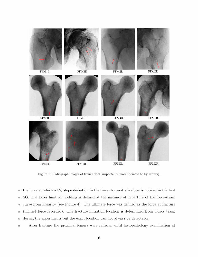
Figure 1: Radiograph images of femurs with suspected tumors (pointed to by arrows).

the force at which a 5% slope deviation in the linear force-strain slope is noticed in the first77

SG. The lower limit for yielding is defined at the instance of departure of the force-strain78

curve from linearity (see Figure 4). The ultimate force was defined as the force at fracture79

(highest force recorded). The fracture initiation location is determined from videos taken80

during the experiments but the exact location can not always be detectable.81

After fracture the proximal femurs were refrozen until histopathology examination at82

6

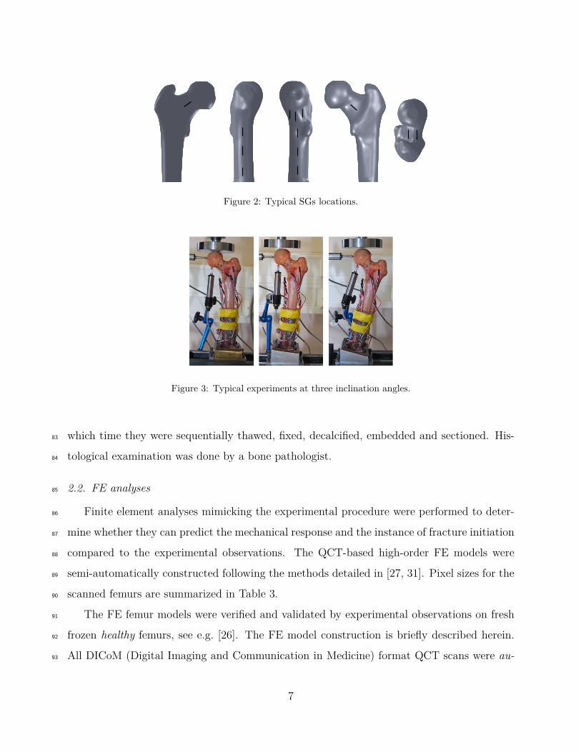
Figure 2: Typical SGs locations.

Figure 3: Typical experiments at three inclination angles.

which time they were sequentially thawed, fixed, decalcified, embedded and sectioned. His-83

tological examination was done by a bone pathologist.84

2.2. FE analyses85

Finite element analyses mimicking the experimental procedure were performed to deter-86

mine whether they can predict the mechanical response and the instance of fracture initiation87

compared to the experimental observations. The QCT-based high-order FE models were88

semi-automatically constructed following the methods detailed in [27, 31]. Pixel sizes for the89

scanned femurs are summarized in Table 3.90

The FE femur models were verified and validated by experimental observations on fresh91

frozen healthy femurs, see e.g. [26]. The FE model construction is briefly described herein.92

All DICoM (Digital Imaging and Communication in Medicine) format QCT scans were au-93

7

Figure 4: Typical graph for determining yield load.

Femur Label FFM1R FFM2R FFM3R FFM4R FFM5R FFM6R FFM7R

Pixel Size (mm) 0.2373 0.2392 0.1953 0.1953 0.2461 0.2314 0.1953

Femur Label FFM1L FFM2L FFM3L FFM4L FFM5L FFM6L FFM7L

Pixel Size (mm) 0.2119 0.2441 0.1953 0.1953 0.2353 0.2561 0.2617

Table 3: CT pixel size for each femur.

tomatically manipulated by in-house Matlab programs. The proximal femur bone’s axis was94

aligned with the z axis. Since no exact Hounsfield Units (HU) exist that distinguish between95

the cortical and trabecular bone we associated values of HU> 475 (ρash > 0.486 g/cm3) with96

the cortical bone and values of HU≤ 475 to trabecular bone according to [1, 6, 8, 2]. CT97

data was manipulated by a 3-D smoothing algorithm that generates clouds of points each98

representing the femur’s exterior, interface and interior boundaries. These clouds of points99

were imported into the CAD package SolidWorks1 that generated a surface representation100

of the femur and subsequently a solid model. The resulting 3D solid was imported into a101

high-order FE code where a tetrahedral FE mesh was created and mesh refined at areas of102

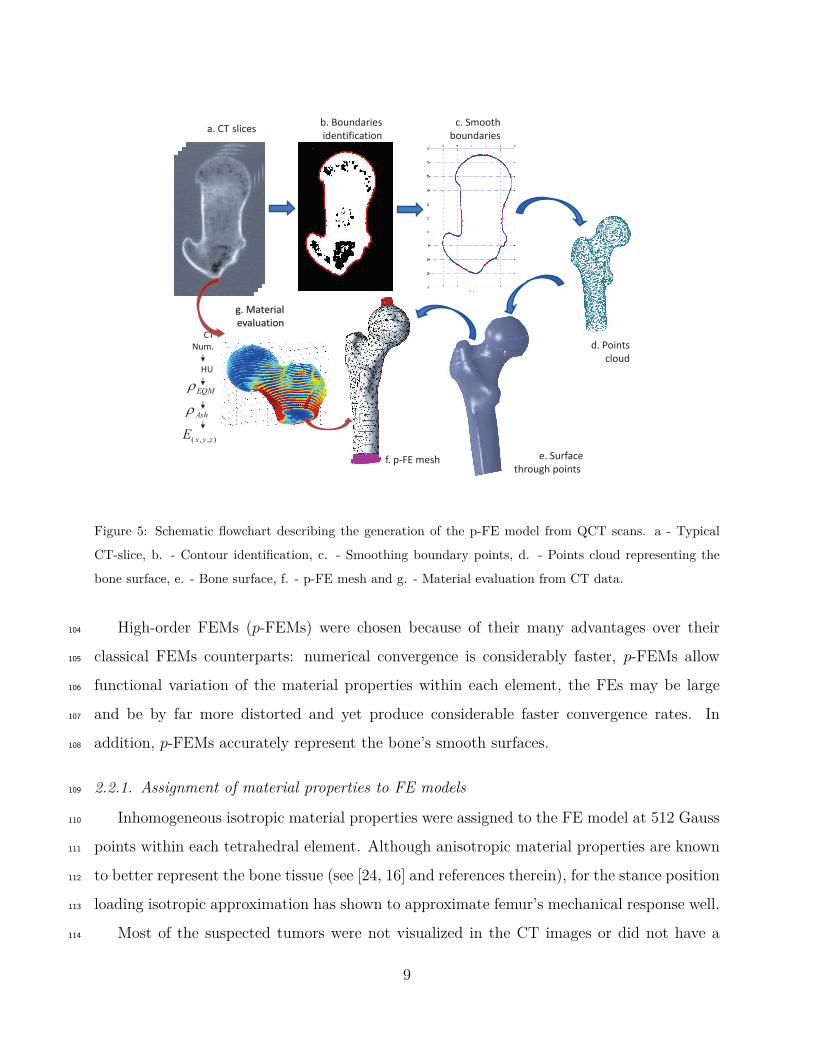
interest. The entire algorithm (QCT to FE model) is schematically illustrated in Figure 5.103

1A CAD (computer-aided design) program developed by Dassault Systems SolidWorks Corp.

8

slices a. CT c. Smooth

boundaries

b. Boundaries

identification

d. Points

cloud

f. p-FE mesh e. Surface

through points

CT

Num.

HU

EQMr

Ashr

),,( zyxE

g. Material

evaluation

Figure 5: Schematic flowchart describing the generation of the p-FE model from QCT scans. a - Typical

CT-slice, b. - Contour identification, c. - Smoothing boundary points, d. - Points cloud representing the

bone surface, e. - Bone surface, f. - p-FE mesh and g. - Material evaluation from CT data.

High-order FEMs (p-FEMs) were chosen because of their many advantages over their104

classical FEMs counterparts: numerical convergence is considerably faster, p-FEMs allow105

functional variation of the material properties within each element, the FEs may be large106

and be by far more distorted and yet produce considerable faster convergence rates. In107

addition, p-FEMs accurately represent the bone’s smooth surfaces.108

2.2.1. Assignment of material properties to FE models109

Inhomogeneous isotropic material properties were assigned to the FE model at 512 Gauss110

points within each tetrahedral element. Although anisotropic material properties are known111

to better represent the bone tissue (see [24, 16] and references therein), for the stance position112

loading isotropic approximation has shown to approximate femur’s mechanical response well.113

Most of the suspected tumors were not visualized in the CT images or did not have a114

9

well defined boundary. Therefore, the tumors were assigned the same material properties115

(according to their mineral bone density) as any other bone tissue in the FE model. This116

methodology has already been identified as appropriate in [14]: “It is important that these117

relationships be applicable to bone with and without metastases because it is difficult to reliably118

identify specific areas of metastatic involvement in a bone. Therefore, instead of applying119

different mechanical property relationships to areas with and without metastatic involvement,120

the relationships presented here can be applied universally throughout. The levels of precision121

and accuracy achieved in this study indicate that this methodology was successful and shows122

the robustness of this modeling method.”123

K2HPO4 liquid phantoms [17] were placed near each femur while immersed in water124

during the CT scan. These phantoms were used to correlate the known mineral density and125

HUs:126

ρK2HP O4 [gr/cm3] = 10−3 × (0.8072 × HU − 1.6) (1)

The ash density ρash is determined based on recent empirical connections [20], using the127

connection between hydroxyapetite and K2HPO4 phantoms [7]:128

ρash [gr/cm3] = 0.877 × 1.21 × ρK2HP O4 + 0.08 (2)

The relation reported in [11] includes specimens with a wide density range (0.092 < ρash <129

1.22 [g/cm3]) while the relation reported in [12] was obtained using ash densities < 0.3 [g/cm3].130

The ρash threshold between cortical and trabecular tissues is unclear, however all the pix-131

els having HU number larger than 475 are considered cortical bone. HU=475 leads to132

ρash = 0.486 using (1) and (2) based on previous publications [29, 31, 10]. Thus, the following133

relations were used to determine Young’s modulus from ρash:134

Ecort = 10200 × ρ2.01ash [MPa], ρash ≥ 0.486 (3)

Etrab = 2398 [MPa], 0.3 < ρash < 0.486 (4)

Etrab = 33900 × ρ2.2ash [MPa], ρash ≤ 0.3 (5)

10

Young’s modulus at the transition area between cortical and trabecular bone tissue ( 0.3 <135

ρash < 0.486) was set to E = 2398 [MPa], based on the data reported in the literature.136

Poisson ratio was set to ν = 0.3.137

2.2.2. Boundary conditions and post-processing of FE results138

To mimic the experimental setup, a compression force of 1000 N was applied on a planar139

circular area (10mm diameter) at the superior surface of the femoral head (see Figure 6) at140

the respective angles (0◦, 7◦ and 15◦). The FE models for all specimens were fully constrained141

at the distal part of the shaft. Since femurs undergo linear mechanical response under small142

strains, only linear analyses were performed. The creation of each model took approximately143

two hours and their solution about eight hours on average.144

(a) (b) (c)

Figure 6: Boundary conditions on the FE models (a)0◦ (b) 7◦ (c) 15◦.

The p-FE models were solved by increasing the polynomial degree until convergence in145

energy norm was observed (all models had an error in energy norm of < 10%). Thereafter,146

verification of convergence was performed to all strains and displacement at the regions147

of interest. In case of poor local convergence, a local refinement and a new analysis was148

performed.149

The average strain along element edges was extracted from FE results since it best repre-150

sents the average strain surface recorded by the SGs. Displacements were extracted at nodes.151

Because uni-axial SGs were used in all experiments, the FE strain component was considered152

in the direction coinciding with the SG direction, which usually were aligned along the local153

11

principal strain directions (E1 or E3). If the SG was found not to align with the principal154

strain, a local axis system was positioned and the value was extracted relatively to the new155

system.156

The predictability of the finite element analyses was examined by comparing the FEA157

results with the experimental observations. Statistical analysis is based on a standard linear158

regression, where a perfect correlation is evident by a unit slope, a zero intercept and a unit159

R2 (linear correlation coefficient). The results are shown also in a Bland-Altman error plot160

((EXP − FE), EXP −F E2 ). The mean error and the absolute mean error values were also161

calculated:162

Mean Error = 100N

ΣNi=1(Exp(i) − FE(i))/Exp(i) [%] (6)

163

Mean absolute Error = 100N

ΣNi=1

∣∣∣(Exp(i) − FE(i))/Exp(i)

∣∣∣ [%] (7)

Predicting yield force: A simplified yield strain criterion, previously shown to predict the164

yield of healthy fresh frozen femurs reasonably well in [29], was used herein to estimate the165

yield of the cancer affected femurs. This criterion estimates the yield initiation to occur166

at the location where the largest principal strain (by a linear elastic analysis) on bone’s167

surface reaches a critical value of 7300 µstrains in tension or -10400 µstrains in compression168

(reported in [2]). The principal strains on femur’s surface were computed for an applied169

1000 N . The ratio between the critical strain in tension (respectively compression) to the170

maximum (respectively minimum) computed principal strain times 1000 N was determined as171

the predicted yield force. Because pointwise values of FE strains may contain large numerical172

errors, we used instead an averaged value along a part of an element edge adjacent to the173

maximum strain location.174

3. Results175

3.1. Experimental results176

Strains and displacements recorded during the mechanical tests showed a linear relation-177

ship with the applied load (excluding the fracture experiments) as shown by a typical example178

12

0 500 10000

100

200

300

400

500

600

700

Str

ain

[µ

str

ain

]

FFM5R�SG10: 0°

ExpA: m=0.79349, R2=0.99

ExpB: m=0.79122, R2=0.99

ExpC: m=0.80416, R2=0.99

ExpD: m=0.86762, R2=0.99

ExpE: m=0.87256, R2=0.99

ExpF: m=0.82902, R2=0.99

0 1000 20000

100

200

300

400

500

600

700

Force [N]

FFM5R�SG10: 7°

ExpA: m=0.5699, R2=0.99

ExpB: m=0.57231, R2=0.99

ExpC: m=0.57024, R2=0.99

ExpD: m=0.67648, R2=0.99

ExpE: m=0.63177, R2=0.99

ExpF: m=0.63201, R2=0.99

0 1000 200050

100

150

200

250

300

350

400

450

FFM5R�SG10: 15°

ExpA: m=0.42013, R2=0.98

ExpB: m=0.41763, R2=0.98

ExpC: m=0.41494, R2=0.98

ExpD: m=0.41903, R2=0.99

ExpE: m=0.41636, R2=0.99

ExpF: m=0.41531, R2=0.99

Figure 7: Typical strain gauge response for the three angles (FFM5R-SG10).

in Figure 7. A non-typical response was noticed for the FFM2 pair, i.e. an increase in strains179

with an increase in the femoral inclination angle. This response was not previously noted180

in any of our prior experiments on 31 femoral specimens. Therefore the FFM2 results were181

excluded with the belief that they represented an experimental error.182

Following the elastic experiments, all fourteen femurs were loaded to failure at an inclined183

angle of 15 degrees while their response was monitored (one femur, FFM4L was accidentally184

fractured at 7◦). Except for the two femurs FFM1R and FFM1L that did not break after185

applying 12,000 N, all other femurs broke at much lower loads. On FFM1R and FFM1L186

the applied displacement on femurs head was maintained for 8-13 seconds during which the187

femurs broke suddenly showing a creep-like phenomenon. Details are provided in [28]. A188

summary of the fracture experiments is given in Table 4. Most of the femurs showed a small189

plastic deformation before fracturing (yield loads were smaller than fracture loads).190

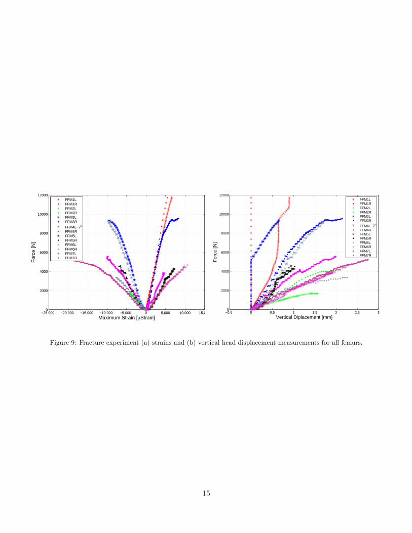
Figure 8 presents the fracture patterns in the femurs. Figure 9 presents the applied force191

vis. measured strain at the SG closest to the failure location and head’s displacement until192

fracture.193

13

Figure 8: Fracture patterns in femurs.

All fractured surfaces underwent histopathology examination and in 8 of the 14 femurs194

metastatic tumors were found (Figure 10).195

14

−25,000 −20,000 −15,000 −10,000 −5,000 0 5,000 10,000 15,0000

2000

4000

6000

8000

10000

12000

Maximum Strain [µStrain]

For

ce [N

]

FFM1LFFM1RFFM2LFFM2RFFM3LFFM3R

FFM4L−7o

FFM4RFFM5LFFM5RFFM6LFFM6RFFM7LFFM7R

−0.5 0 0.5 1 1.5 2 2.5 30

2000

4000

6000

8000

10000

12000

Vertical Diplacement [mm]

For

ce [N

]

FFM1LFFM1RFFM2LFFM2RFFM3LFFM3R

FFM4L−7o

FFM4RFFM5LFFM5RFFM6LFFM6RFFM7LFFM7R

Figure 9: Fracture experiment (a) strains and (b) vertical head displacement measurements for all femurs.

15

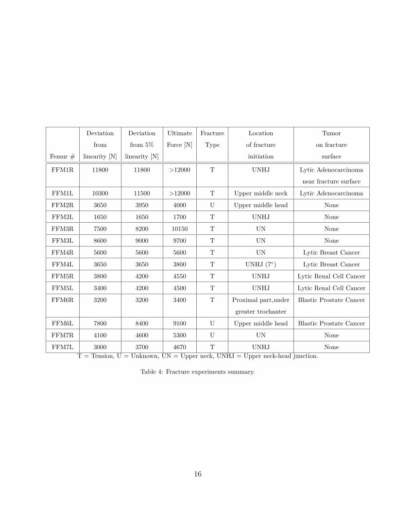
Deviation Deviation Ultimate Fracture Location Tumor

from from 5% Force [N] Type of fracture on fracture

Femur # linearity [N] linearity [N] initiation surface

FFM1R 11800 11800 >12000 T UNHJ Lytic Adenocarcinoma

near fracture surface

FFM1L 10300 11500 >12000 T Upper middle neck Lytic Adenocarcinoma

FFM2R 3650 3950 4000 U Upper middle head None

FFM2L 1650 1650 1700 T UNHJ None

FFM3R 7500 8200 10150 T UN None

FFM3L 8600 9000 9700 T UN None

FFM4R 5600 5600 5600 T UN Lytic Breast Cancer

FFM4L 3650 3650 3800 T UNHJ (7◦) Lytic Breast Cancer

FFM5R 3800 4200 4550 T UNHJ Lytic Renal Cell Cancer

FFM5L 3400 4200 4500 T UNHJ Lytic Renal Cell Cancer

FFM6R 3200 3200 3400 T Proximal part,under Blastic Prostate Cancer

greater trochanter

FFM6L 7800 8400 9100 U Upper middle head Blastic Prostate Cancer

FFM7R 4100 4600 5300 U UN None

FFM7L 3000 3700 4670 T UNHJ NoneT = Tension, U = Unknown, UN = Upper neck, UNHJ = Upper neck-head junction.

Table 4: Fracture experiments summary.

16

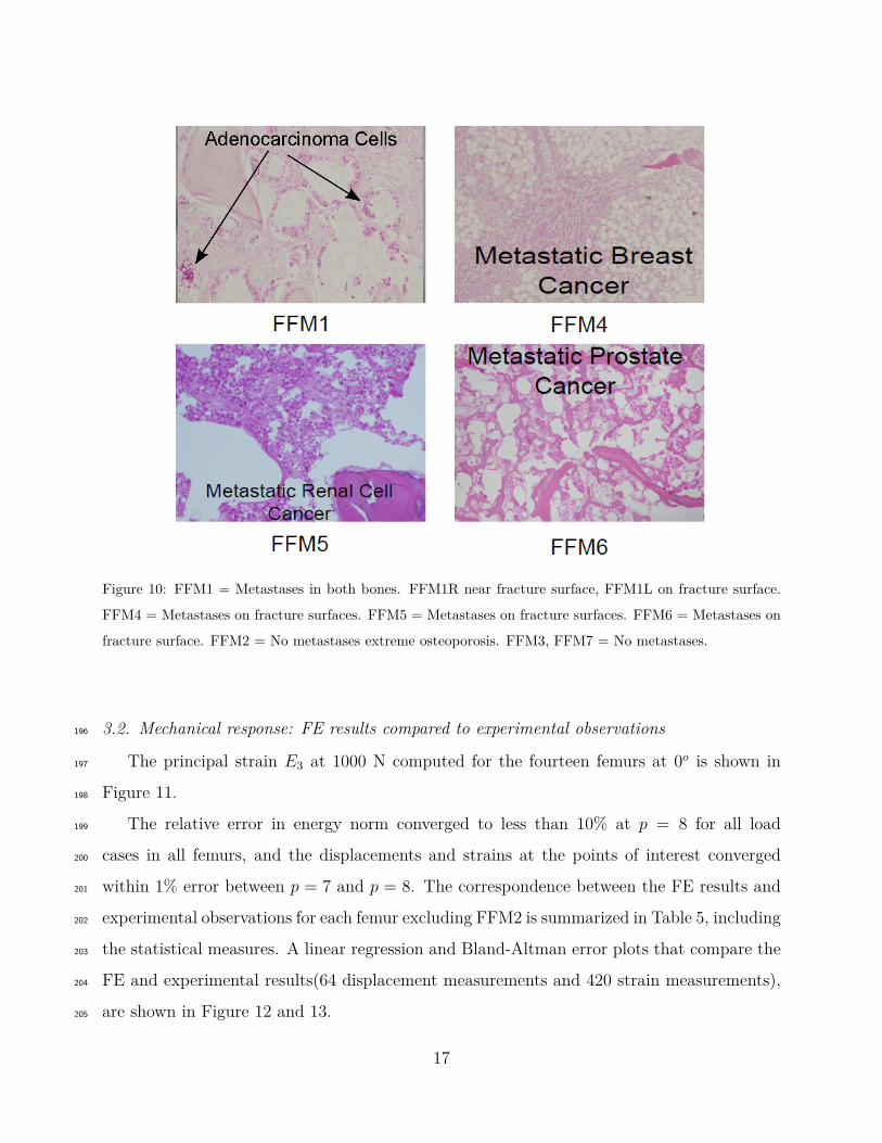
Figure 10: FFM1 = Metastases in both bones. FFM1R near fracture surface, FFM1L on fracture surface.

FFM4 = Metastases on fracture surfaces. FFM5 = Metastases on fracture surfaces. FFM6 = Metastases on

fracture surface. FFM2 = No metastases extreme osteoporosis. FFM3, FFM7 = No metastases.

3.2. Mechanical response: FE results compared to experimental observations196

The principal strain E3 at 1000 N computed for the fourteen femurs at 0o is shown in197

Figure 11.198

The relative error in energy norm converged to less than 10% at p = 8 for all load199

cases in all femurs, and the displacements and strains at the points of interest converged200

within 1% error between p = 7 and p = 8. The correspondence between the FE results and201

experimental observations for each femur excluding FFM2 is summarized in Table 5, including202

the statistical measures. A linear regression and Bland-Altman error plots that compare the203

FE and experimental results(64 displacement measurements and 420 strain measurements),204

are shown in Figure 12 and 13.205

17

FFM1R

FFM3R

FFM1L

FFM3L

FFM5R FFM5L

FFM2R FFM2L

FFM4R FFM4L

FFM6LFFM6R

FFM7R FFM7L

Figure 11: Principal strain E3 at 1000 N load computed by p-FE analyses for the fourteen femurs at 0o

inclination (colors not at same scales for all models).

18

Bone (label) Linear Correlation R2 Mean error (%) Mean absolute error (%)

FFM1R FE= 1.059 × EXP+2.96 0.982 -4 14

FFM1L FE=0.956 × EXP-9.30 0.976 -2 13

FFM3R FE=0.935 × EXP-2.79 0.951 0 14

FFM3L FE=1.016 × EXP-0.68 0.981 -5 14

FFM4R FE=0.917 × EXP+33.05 0.981 -1 15

FFM4L FE=1.038 × EXP+34.86 0.980 -12 15

FFM5R FE=0.997 × EXP+16.35 0.992 -2 14

FFM5L FE=0.926 × EXP-19.74 0.990 -9 8

FFM6R FE=0.838 × EXP-51.53 0.952 9 19

FFM6L FE=0.960 × EXP-0.70 0.982 -2 12

FFM7R FE=1.096 × EXP-153.0 0.946 -13 23

FFM7L FE=0.950 × EXP-103.3 0.980 13 16

All FE=0.949 × EXP-25 0.957 -0.8 14.8

Table 5: Summary of statistical measures for the biomechanical response of the individual femurs.

−4000 −3000 −2000 −1000 0 1000 2000 3000 4000−4000

−3000

−2000

−1000

0

1000

2000

3000

EXP

FE

Strains [µstrains]Displacements [µm]

0.9493*EXP−25.02, R2=0.957

Figure 12: Linear correlation for all biomechanical data excluding FFM2 (strains and displacements on

femurs’ boundaries).

19

−3000 −2000 −1000 0 1000 2000 3000

−1500

−1000

−500

0

500

1000

1500

Average [N]

Diff

eren

ce (

Exp

−F

EA

)

Strains [µstrains]Displacement [µm]MeanMean ± 1.96SD

Figure 13: Bland-Altman error plot for all biomechanical data excluding FFM2 (strains and displacements

on femurs’ boundaries).

20

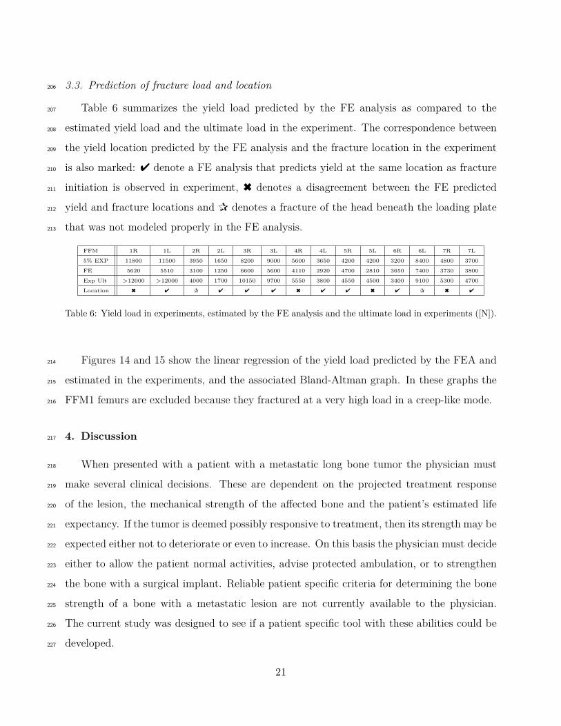
3.3. Prediction of fracture load and location206

Table 6 summarizes the yield load predicted by the FE analysis as compared to the207

estimated yield load and the ultimate load in the experiment. The correspondence between208

the yield location predicted by the FE analysis and the fracture location in the experiment209

is also marked: 4 denote a FE analysis that predicts yield at the same location as fracture210

initiation is observed in experiment, 6 denotes a disagreement between the FE predicted211

yield and fracture locations and P denotes a fracture of the head beneath the loading plate212

that was not modeled properly in the FE analysis.213

FFM 1R 1L 2R 2L 3R 3L 4R 4L 5R 5L 6R 6L 7R 7L

5% EXP 11800 11500 3950 1650 8200 9000 5600 3650 4200 4200 3200 8400 4800 3700

FE 5620 5510 3100 1250 6600 5600 4110 2920 4700 2810 3650 7400 3730 3800

Exp Ult >12000 >12000 4000 1700 10150 9700 5550 3800 4550 4500 3400 9100 5300 4700

Location 6 4 P 4 4 4 6 4 4 6 4 P 6 4

Table 6: Yield load in experiments, estimated by the FE analysis and the ultimate load in experiments ([N]).

Figures 14 and 15 show the linear regression of the yield load predicted by the FEA and214

estimated in the experiments, and the associated Bland-Altman graph. In these graphs the215

FFM1 femurs are excluded because they fractured at a very high load in a creep-like mode.216

4. Discussion217

When presented with a patient with a metastatic long bone tumor the physician must218

make several clinical decisions. These are dependent on the projected treatment response219

of the lesion, the mechanical strength of the affected bone and the patient’s estimated life220

expectancy. If the tumor is deemed possibly responsive to treatment, then its strength may be221

expected either not to deteriorate or even to increase. On this basis the physician must decide222

either to allow the patient normal activities, advise protected ambulation, or to strengthen223

the bone with a surgical implant. Reliable patient specific criteria for determining the bone224

strength of a bone with a metastatic lesion are not currently available to the physician.225

The current study was designed to see if a patient specific tool with these abilities could be226

developed.227

21

0 1000 2000 3000 4000 5000 6000 7000 8000 9000 10000 110000

1000

2000

3000

4000

5000

6000

7000

8000

Exp. Yield Force− 5% slope linear deviation

FE

Yie

ld F

orce

Break Force [N]Yield Force [N]

FE=0.797EXP ,R2=0.78

Figure 14: Linear correlation for yield load excluding FFM1.

Figure 15: Bland-Altman error plot for yield load excluding FFM1.

The use of patient specific CT-based p-FEA to predict the biomechanical response of228

healthy femurs has been demonstrated to provide excellent results [30, 26]. Leveraging on229

this capability, a natural question was raised whether CT-based p-FEA may be applied with230

22

the same success to femurs with metastatic tumors. To the best of our knowledge, this is the231

first work that investigates the mechanical response of femurs with actual metastatic tumors.232

Femurs with metastatic tumors are of major concern due to the risk of spontaneous233

pathological fractures, that may occur during activities of daily living. For this reason, we234

considered loads that were applied to the femoral head that mimic stance position. We235

performed mechanical experiments and FE analyses on a large cohort of fourteen femurs236

suspected to contain metastatic tumors. This is the largest cohort of such femurs among237

previous publications on the topic: in [23, 5] ten femurs (healthy with holes that mimic238

metastatic tumors) were considered, and in [13] twelve femurs with metastatic tumors were239

considered.240

The predicted strains and displacements showed an excellent agreement with the exper-241

imental observations with a linear regression slope of 0.95 and a coefficient of regression R2242

= 0.967. In the analysis of the mechanical response the pair of femurs FFM2 was excluded243

because of an unusual experimental response that can be attributed to experimental errors.244

Altogether 420 strains and 64 displacements from twelve femurs were analyzed.245

Since most of the suspected tumors were not recognized in the CT images or did not have246

a well defined boundary, the same density-material properties relations as any other bone247

tissue was assigned to them in the FE model (as in [14]). These results suggest that there is248

no need for a special tumor E-ρash relationship since the effect of metastases is accounted for249

due to density changes. Even though most of the tumors were not visible in the CT scans,250

the FE models provided good results. This implies that CT based p-FEMs are capable of251

predicting the mechanical response of femurs without knowledge of tumor’s presence or tumor252

specifically representation. The wide diversity of tumor (blastic, lytic and mixed) and cancer253

types involved in this work contributed to the reliability of the proposed methodology.254

The results also emphasized that drilling holes in healthy femurs to mimic metastatic255

tumors, as reported in several past publications, may not well represent actual metastatic256

tumors in bones.257

Our FE predictions were considerably better for strains than for displacements. This258

is because we clamped the distal part of the femur in the FE analysis so that the FE dis-259

23

placements were smaller compared to the ones measured in the experiment where the bone’s260

distal part was embedded into PMMA and had some elastic displacement (this observa-261

tion was confirmed by other FEA and experiments lately performed by the authors). The262

Bland-Altman plot in Figure 13 shows that the mean is unbiased, and 95% of the computed263

strains are within ±500µstrain of the measured ones within the range ±3000µstrains. The264

mean (6) and absolute mean (7) errors for the overall results (excluding FFM2) are -1%265

and 14.8%, respectively. The differences between the predicted and measured strains and266

displacements are considered low compared with past studies, especially for the fresh frozen267

femurs in this work that were affected by malignant tumors. In general, the FE predictions268

provided slightly smaller values than the measured ones, implying that the femur FE models269

are slightly stiffer compared to the actual femurs, possibly because of the weakened femurs270

due to the metastatic tumors.271

Regarding the prediction of the risk of bone yielding (a non-reversible damage accumu-272

lated in the bone tissue), all past publications that use FEA for the determination of fracture273

onset in femurs with metastases based their predictions on some sort of stress-criterion. How-274

ever, the use of FE stresses necessitates first ensuring that the computed stresses are accurate275

and correlated to in-vitro experiments before being used to determine any fracture instance.276

To the best of our understanding, past FE stresses were not compared to any experimental ob-277

servations to demonstrate their validity. Furthermore, there is no evidence that stress-based278

fracture criterion (usually the von-Mises yield criterion) are appropriate for bone tissue.279

In this research, we used a simplified yield strain criterion [29] to estimate the yield of280

the cancer affected femurs. Excluding the pair of femurs FFM1R and FFM1L, that fractured281

under a creep phenomenon after applying over 12000 N, we demonstrated a good correlation282

between the predicted yield load and the experimental observed yield, with a linear regression283

slope of 0.80 and a coefficient of regression R2 = 0.78. In almost all cases the predicted yield284

load was lower compared to the experiment, demonstrating the conservative prediction (i.e.285

should the criterion be used in clinical practice, the yield is predicted before the femur yields).286

Notice that yield load almost coincides with the ultimate load for femurs that fractured287

24

at relatively low loads, and that the FE predictions for these cases are relatively accurate.288

This is of great clinical importance because only for these femurs is it important to accurately289

predict the risk of yielding, whereas there is no biomechanical concern for femurs that have290

large predicted yield loads.291

In eight of the fourteen femurs the fracture surface passed through the metastatic tumor292

or very close to it. The metastatic tumor in seven out of the eight femurs was confined to293

the cancellous portion of the femur and not in the cortex. Pathology results showed that294

metastases to the bone have a significant influence on the fracture location, no matter what295

type of tumors (lytic or blastic) or type of cancer is present. The only femur that had a296

clearly demonstrated large tumor in the cortex (FFM6R), was clearly identified by the FE297

analysis to fail at the location of the tumor. For this case the FE predicted yielding load298

was 14% beyond the experimental yield load and 7% beyond the experimental fracture load.299

Although the FE analysis over-estimated the yield load, a very good yield prediction was300

noticed even for these highly compromised femurs.301

Although the experimental yield forces were within a broad range (1700 to 10000 [N])302

the predicted yield force were reasonably accurate, and for the low yield forces (less than303

6000 [N]) a very good prediction was obtained. These results for a simple linear model as304

presented here are satisfactory for clinical usage. The predicted locations are accurate in 8305

out of 14 fracture locations. Two (FFM2R and FFM6L) of the unsuccessful predictions were306

due to a fracture occurring in the middle of the head, close to the load application by the307

flat machine punch. Since FE models in the vicinity of the load did not mimic precisely the308

experimental setting (load was applied instead of a constant displacement on a flat surface),309

it is not surprising that these fracture patterns were not accurately predicted.310

Analysis of the specific tumors at the fracture surfaces: FFM1, FFM4 and FFM5 showed311

lytic and FFM6 showed blastic tumors in their fracture surfaces, being probably a significant312

factor in the location of the fractures. FFM6R fractured through a significant tumor located313

under the greater trochanter suggesting that cortical involvement of the tumor plays an314

important role in the fracture site and load. When comparing to FFM6L, one may observe315

that metastasis in FFM6R was considerably more aggressive (this is visible in the X-rays316

25

images and in the CT scans) significantly affecting its bearing capacity. Lytic metastases317

of adenocarcinoma2 tumors were found in the two FFM1 femurs. It was found close to the318

fracture surface of the right FFM1 femur, and on the fracture surface in the left FFM1 femur.319

In the right side the tumor was much smaller. FFM1 femurs showed no reduction in their320

bearing capacity due to the presence of tumors, but the fracture location was affected.321

One may observe that the fracture force of FFM2L is considerably lower than the other322

thirteen femurs. This is a consequence of extreme osteoporosis in the femur. On the other323

hand, the relatively large head displacement of FFM2L may indicate that the bone suffered324

significant plastic deformation until fracture. In these femurs the predicted yield load is325

20-25% lower compared to the experiments. Although such predictions may be considered326

adequate for clinical applications, further investigation is planned to address such osteoporotic327

bones.328

There are several limitations to the present study: a) A single and simplified stance po-329

sition loading was applied (at three different inclination angles). More loading conditions330

will be applied in future studies. b) The bone tissue is inhomogeneous orthotropic or trans-331

versely isotropic and the application of inhomogeneous isotropic material properties in the332

FE simulations is a simplification of the reality. For a more complex state of loading, more333

realistic material properties would probably result in a better correlation with the in-vitro334

experiments. c) More sophisticated yield laws for the bone tissue, with parameters that can335

be measured by clinical procedures are lacking. These should be developed to include also336

the influence of the type of metastatic tumor on the yield law.337

This study shows that the FEM method previously validated to estimate the strength338

of the proximal femur can also be used for estimations when metastatic lesions are present.339

For the method to be used as a clinical tool, further development is necessary. The time for340

creating the FE model and the processing time need to be automated and shortened. The341

technique has to be validated for additional bone anatomical sites and other clinical situations342

2Metastases of cancer from a glandular tissue.

26

such as fractures. The economic cost for the service has to be delivered at a reasonable price.343

Additional, adapting it to a hand held communication device would make use of the method344

convenient to the clinician.345

Conflict of Interest346

None of the authors have any conflict of interest to declare that could bias the presented347

work.348

Acknowledgements349

The authors thank Mr. Ilan Gilad and Natan Levin from the Ben-Gurion University of the350

Negev, Israel, for their help with the experiments. The first author gratefully acknowledges351

the generous support of the Technical University of Munich - Institute for Advanced Study,352

funded by the German Excellence Initiative. This study was supported in part by grant no.353

3-00000-7375 from the Chief Scientist Office of the Ministry of Health, Israel.354

References355

[1] A. Alho, T. Husby, and A. Hoiseth. Bone mineral content and mechanical strength. An356

ex-vivo study on human femora and autopsy. Clin. Orthop., 227:292–297, 1988.357

[2] H.H. Bayraktar, E.F. Morgan, G.L. Niebur, G.E. Morris, E.K. Wong, and M. Keaveny.358

Comparison of the elastic and yield properties of human femoral trabecular and cortical359

bone tissue. Jour. Biomech., 37:27–35, 2004.360

[3] R. E. Coleman. Clinical features of metastatic boned isease and risk of skeletal morbidity.361

Clinical Cancer Research, 12:6243s–6249s, 2006.362

[4] T.A. Damron, H. Morgan, D. Prakash, W. Grant, J. Aronowitz, and J. Heiner. Critical363

evaluation of Mirels rating system for impending pathologic fractures. Clin. Orthop.364

Relat. Res., 415:S201–S207, 2003.365

[5] L. C. Derikx, J. B. van Aken, D. Janssen, A. Snyers, Y. M. van der Linden, N. Verdon-366

schot, and E. Tanck. The assessment of the risk of fracture in femora with metastatic367

27

lesions: Comparing case-specific finite element analyses with predictions by clinical ex-368

perts. Jour. Bone Joint Surg., 94-B(8):1135–1142, 2012.369

[6] SI. Esses, JC. Lotz, and WC. Hayes. Biomechanical properties of the proximal femur370

determined in vitro by single-energy quantitative computed tomography. Jour. Bone371

Mineral Res., 4:715–722, 1989.372

[7] M.M Goodsitt. Conversion relations for quantitative ct bone mineral densities measured373

with solid and liquid calibration standards. Bone. and. Mineral, 19:145–158, 1992.374

[8] B. J. Heismann, J. Leppert, and K. Stierstorfer. Density and atomic number measure-375

ments with spectral x-ray attenuation method. J. App. Phys., 94:2073–2079, 2003.376

[9] Muhammad Umar Jawad and Sean P. Scully. In brief: Classifications in brief: Mirels’377

classification: Metastatic disease in long bones and impending pathologic fracture. Clin.378

Orthop. Relat. Res., 468(10), 2010.379

[10] Alon Katz. The mechanical response of femurs fixed by metal devices. MSc thesis, Dept.380

of Mechanical Engineering, Ben-Gurion University of the Negev, Beer-Sheva, Israel,381

2011.382

[11] T. S. Keller. Predicting the compressive mechanical behavior of bone. Jour. Biomech.,383

27:1159–1168, 1994.384

[12] J.H . Keyak, M. G. Fourkas, J. M. Meagher, and H. B. Skinner. Validation of automated385

method of three-dimensional finite element modelling of bone. ASME Jour. Biomech.386

Eng., 15:505–509, 1993.387

[13] JH Keyak, TS Kaneko, SA Rossi, MR Pejcic, J Tehranzadeh, and HB Skinner. Predicting388

the strength of femoral shafts with and without metastatic lesions. Clin. Orthop. Relat.389

Res., 439:161–170, 2005.390

[14] JH Keyak, TS Kaneko, J Tehranzadeh, and HB Skinner. Predicting proximal femoral391

28

strength using structural engineering models. Clin. Orthop. Relat. Res., 437:219–228,392

2005.393

[15] Kenneth A. Mann, John Lee, Sarah A. Arrington, Timothy A. Damron, and Matthew J.394

Allen. Predicting distal femur bone strength in a murine model of tumor osteolysis. Clin.395

Orthop. Relat. Res., 466(6):1271–1278, 2008.396

[16] Javad Hazrati Marangalou, Keita Ito, and Bert van Rietbergen. A new approach to397

determine the accuracy of morphology-elasticity relationships in continuum FE analyses398

of human proximal femur. Jour. Biomech., 45(16):2884–2892, 2012.399

[17] Mindways Software, 282 Second St., San Francisco, CA 94105. CT Calibration Phantom,400

2002.401

[18] H. Mirels. Metastatic disease in long bones. a proposed scoring system for diagnosing402

impending pathologic fractures. Clin. Orthop. Relat. Res., 249:256–264, 1989.403

[19] John A. Rennick, Ara Nazarian, Vahid Entezari, James Kimbaris, Alan Tseng, Aidin404

Masoudi, Hamid Nayeb-Hashemi, Ashkan Vaziri, and Brian D. Snyder. Finite element405

analysis and computed tomography based structural rigidity analysis of rat tibia with406

simulated lytic defects. Jour. Biomech., 46(15):2701 – 2709, 2013.407

[20] E. Schileo, E. DallAra, F. Taddei, A. Malandrino, T. Schotkamp, M. Baleani, and408

M. Viceconti. An accurate estimation of bone density improves the accuracy of subject-409

specific finite element models. Jour. Biomech., 41:2483–2491, 2008.410

[21] Brian D. Snyder, Marsha A. Cordio, Ara Nazarian, S. Daniel Kwak, David J. Chang,411

Vahid Entezari, David Zurakowski, and Leroy M. Parker. Noninvasive prediction of412

fracture risk in patients with metastatic cancer to the spine. Clin. Cancer Research,413

15(24):7676–7683, 2009.414

[22] Sander Spruijt, Jacqueline C Van Der Linden, P D Sander Dijkstra, Theo Wiggers,415

Mathijs Oudkerk, Chris J Snijders, Fred Van Keulen, Jan A N Verhaar, Harrie Weinans,416

29

and Bart A Swierstra. Prediction of torsional failure in 22 cadaver femora with and417

without simulated subtrochanteric metastatic defects: A CT scan-based finite element418

analysis. Acta Orthopaedica, 77(3):474–481, 2006.419

[23] Esther Tanck, Jantien B. van Aken, Yvette M. van der Linden, H.W. Bart Schreuder,420

Marcin Binkowski, Henk Huizenga, and Nico Verdonschot. Pathological fracture pre-421

diction in patients with metastatic lesions can be improved with quantitative computed422

tomography based computer models. Bone, 45(4):777 – 783, 2009.423

[24] N. Trabelsi and Z. Yosibash. Patient-specific FE analyses of the proximal femur with424

orthotropic material properties validated by experiments. ASME Jour. Biomech. Eng.,425

155:061001–1 – 061001–11, 2011.426

[25] N. Trabelsi, Z. Yosibash, and C. Milgrom. Validation of subject-specific automated p-FE427

analysis of the proximal femur. Jour. Biomech., 42:234–241, 2009.428

[26] N. Trabelsi, Z. Yosibash, C. Wutte, R. Augat, and S. Eberle. Patient-specific finite429

element analysis of the human femur - a double-blinded biomechanical validation. Jour.430

Biomech., 44:1666 – 1672, 2011.431

[27] Z. Yosibash, R. Padan, L. Joscowicz, and C. Milgrom. A CT-based high-order finite432

element analysis of the human proximal femur compared to in-vitro experiments. ASME433

Jour. Biomech. Eng., 129(3):297–309, 2007.434

[28] Z. Yosibash, R. Plitman Mayo, and C. Milgrom. Atypical viscous fracture of human435

femurs. Advances in Biomech. & Appl., 1(2):77–83, 2014.436

[29] Z. Yosibash, D. Tal, and N. Trabelsi. Predicting the yield of the proximal femur using437

high order finite element analysis with inhomogeneous orthotropic material properties.438

Philosophycal Transaction of the Royal Society: A, 368:2707–2723, 2010.439

[30] Z. Yosibash, N. Trabelsi, and C. Hellmich. Subject-specific p-FE analysis of the prox-440

imal femur utilizing micromechanics based material properties. Int. Jour. Multiscale441

Computational Engineering, 6(5):483–498, 2008.442

30

[31] Z. Yosibash, N. Trabelsi, and C. Milgrom. Reliable simulations of the human proximal443

femur by high-order finite element analysis validated by experimental observations. Jour.444

Biomech., 40:3688–3699, 2007.445

31