Predicting the global distribution of planktonic ... · PDF filePredicting the global distribution of planktonic foraminifera using a ... ences between modern and fossil species

Biogeosciences, 5, 891–911, 2008www.biogeosciences.net/5/891/2008/© Author(s) 2008. This work is distributed underthe Creative Commons Attribution 3.0 License.

Biogeosciences

Predicting the global distribution of planktonic foraminifera using adynamic ecosystem model

I. Fraile 1, M. Schulz1,2, S. Mulitza2, and M. Kucera3

1Faculty of Geosciences, University of Bremen, P.O. Box 330440, 28334 Bremen, Germany2MARUM – Center For Marine Environmental Sciences, University of Bremen, P.O. Box 330440, 28334 Bremen, Germany3Institute of Geosciences, Eberhard Karls University of Tubingen, Sigwartstrasse 10, 72076 Tubingen, Germany

Received: 17 October 2007 – Published in Biogeosciences Discuss.: 26 November 2007Revised: 7 April 2008 – Accepted: 9 May 2008 – Published: 2 June 2008

Abstract. We present a new planktonic foraminifera modeldeveloped for the global ocean mixed-layer. The main pur-pose of the model is to explore the response of planktonicforaminifera to different boundary conditions in the geolog-ical past, and to quantify the seasonal bias in foraminifera-based paleoceanographic proxy records. This model isforced with hydrographic data and with biological infor-mation taken from an ecosystem model to predict monthlyconcentrations of the most common planktonic foraminiferaspecies used in paleoceanography:N. pachyderma(sinistraland dextral varieties),G. bulloides, G. ruber (white variety)andG. sacculifer. The sensitivity of each species with re-spect to temperature (optimal temperature and range of tol-erance) is derived from previous sediment-trap studies.

Overall, the spatial distribution patterns of most of thespecies are in agreement with core-top data.N. pachy-derma (sin.) is limited to polar regions,N. pachyderma(dex.) andG. bulloidesare the most common species inhigh productivity zones, whileG. ruberandG. sacculiferaremore abundant in tropical and subtropical oligotrophic wa-ters. ForN. pachyderma(sin) andN. pachyderma(dex.), theseason of maximum production coincides with that observedin sediment-trap records. Model and sediment-trap data forG. ruber andG. sacculifershow, in general, lower concen-trations and less seasonal variability at all sites. A sensitiv-ity experiment suggest that, within the temperature-tolerancerange of a species, food availability may be the main param-eter controlling its abundance.

Correspondence to:I. Fraile([email protected])

1 Introduction

Planktonic foraminifera are widely used for paleoceano-graphic reconstructions. The spatial distribution of plank-tonic foraminifera species is controlled by physiological re-quirements, feeding preferences and temperature (e.g.,Beand Hamilton, 1967; Be and Tolderlund, 1971). Shells ofplanktonic foraminifera extracted from marine sedimentsserve as an archive of chemical and physical signals that canbe used to quantify past environmental conditions, such astemperature (e.g.,Pflaumann et al., 1996; Malmgren et al.,2001), ocean stratification (e.g.,Mulitza et al., 1997), at-mospheric CO2 concentration (Pearson and Palmer, 2000)and biological productivity (Kiefer, 1998). Past sea-surfacetemperatures can be estimated by either quantifying differ-ences between modern and fossil species assemblages (e.g.,CLIMAP, 1976; Pflaumann et al., 1996; Malmgren et al.,2001), or by analyzing the isotopic or trace-element com-position of the calcite in the shell (e.g.,Rohling and Cooke,1999; Lea, 1999). In general, all estimation procedures arebased on a correlation between modern environmental con-dition and assemblage composition or shell chemistry.

Seasonal changes in the flux of planktonic foraminifera arestrongly influenced by environmental factors, such as sea-surface temperature, the stratification of the water column,and food supply (e.g.,Bijma et al., 1990; Ortiz et al., 1995;Watkins et al., 1996; Watkins and Mix, 1998; Eguchi et al.,1999; Schnack-Schiel et al., 2001; King and Howard, 2003a;Morey et al., 2005; Zaric et al., 2005). The seasonality offoraminiferal production is an important factor which has tobe taken into account in paleoceanographic interpretations(e.g.,Deuser and Ross, 1989; Wefer, 1989; Mulitza et al.,1998; Ganssen and Kroon, 2000; King and Howard, 2001;

Published by Copernicus Publications on behalf of the European Geosciences Union.

http://creativecommons.org/licenses/by/3.0/

892 I. Fraile et al.: A dynamic global model for planktonic foraminifera

Pflauman et al., 2003; Waelbroeck et al., 2005). Any changein the timing of the seasonal maximum of foraminiferal fluxmay lead to a bias in estimated paleotemperature.Mulitzaet al.(1998) have shown how temperature sensitivity can al-ter the proxy record in the sediment. Moreover, this differ-ences in seasonality make reconstructed temperatures basedon planktonic foraminifera assemblages difficult to comparewith those derived by other sea-surface temperature prox-ies. For example,Niebler et al.(2003) suggested that dis-crepancies between temperature reconstructions based onforaminifera and alkenones might be due to different eco-logical and thus seasonal preferences of alkenone producingalgae and planktonic foraminifera. Climate change could in-duce variations in the seasonal succession of the planktonicforaminifera and such variations need to be quantified to cor-rectly interpret corresponding proxy-based reconstructions.

To study the seasonal variations of planktonic foraminiferaspecies we have developed a numerical model for planktonicforaminifera at a species level. Previously,Zaric et al.(2006)developed an statistical model based on hydrographic andproductivity data. In contrast to the model ofZaric etal. (2006), we present a dynamic model which, consider-ing ecological processes, calculates the growth rate of theforaminifera population between successive time steps. Thisstudy shows model predictions for spatial and temporal dis-tribution patterns of the five most important modern plank-tonic foraminifera used as SST proxies.

2 Model setup

The geographical distribution and population density of eachplanktonic foraminifera species depend on biotic (e.g., food,symbionts) and abiotic factors (e.g., light, temperature). Tosupply the foraminifera model with ecological information,we run the foraminifera module within an ecosystem model.

2.1 Ecosystem model

The employed marine ecosystem model (Moore et al., 2002a)is configured for the global mixed-layer of the ocean. It pre-dicts the distribution of zooplankton, diatoms, diazotrophsand a generic group of phytoplankton (so-called “small phy-toplankton”). The model considers sinking and non-sinkingdetrital pools, and carries nitrate, ammonium, phosphate,iron and silicate as nutrients.

The ecosystem model is driven by hydrographic data thatare derived from a general ocean circulation model and fromclimatologies. The forcing data include local processes ofturbulent mixing, vertical velocity at the base of the mixedlayer, and seasonal mixed-layer entrainment/detrainment.Horizontal advection is not included; thus, there is no lateralexchange between grid points. Since our main interest is theecosystem in the mixed layer, processes below the surfacelayer are ignored.

Previously, this two-dimensional model has been vali-dated against a diverse set of field observations from severalJGOFS (Joint Global Ocean Flux Study) and historical timeseries locations (Moore et al., 2002a), satellite observations,and global nutrient climatologies (Moore et al., 2002b). Thefull list of model terms, parametrizations, resolution, equa-tions and behavior in the global domain is described in de-tail in Moore et al.(2002a,b) and the code is available athttp://usjgofs.whoi.edu/mzweb/jkmoore/areadme.html.

2.2 PLAFOM

The planktonic foraminifera model determines the globaldistribution of the following 5 species:Neogloboquadrinapachyderma(sinistral and dextral coiling varieties),Globige-rina bulloides, Globigerinoides ruber(white variety) andGlobigerinoides sacculifer. These species have often beenconsidered to be sensitive to sea-surface temperature, andtherefore their assemblage can be used to estimate past sea-surface temperatures by means of transfer functions.

Each species has a different food preference (Hemleben etal., 1989; Watkins et al., 1996; Schiebel et al., 1997; Watkinsand Mix, 1998; Arnold and Parker, 1999). In general, spinosespecies prefer animal prey such as copepods (Spindler et al.,1984; Caron and Be, 1984; Hemleben et al., 1989) whilenon-spinose species are largely herbivorous (Anderson et al.,1979; Spindler et al., 1984; Hemleben et al., 1985, 1989),although in some specimens muscle tissue has been foundin food vacuoles (Anderson et al., 1979; Hemleben et al.,1989). Many species also contain algal symbionts that mayprovide nutrition (Caron et al., 1981; Gastrich, 1987; Ortizet al., 1995). On a seasonal scale, it is generally assumedthat food is the predominant factor affecting the distribu-tion of planktonic foraminifera under favorable temperatures(Ortiz et al., 1995). Planktonic foraminifera appear to re-spond to the redistribution of nutrients and phytoplanktonvery quickly, increasing in number of individuals within sev-eral days (Schiebel et al., 1995). Information about foodavailability is obtained from the ecosystem model. In themodel, the food sources may be either zooplankton, smallphytoplankton, diatoms or organic detritus.

For compatibility with the ecosystem model, theforaminifera model calculates foraminiferal abundance ofeach species via carbon biomass, the same as the ecosystemmodel. Since our study is directed to paleotemperature re-constructions, our main interest is in species relative abun-dances rather than in assessing the absolute biomass.

Accordingly, for each species the change in foraminiferaconcentration is calculated as follows:

dF

dt= (GGE· TG) − ML (1)

whereF is the foraminifera carbon concentration, and GGE(gross growth efficiency) is the portion of grazed matter thatis incorporated into foraminifera biomass, which we assume

Biogeosciences, 5, 891–911, 2008 www.biogeosciences.net/5/891/2008/

http://usjgofs.whoi.edu/mzweb/jkmoore/areadme.html

I. Fraile et al.: A dynamic global model for planktonic foraminifera 893

to be constant regardless of the food source. TG and MLrepresent total grazing and mass loss, respectively.

2.2.1 Growth (TG)

The growth rates are determined by available food using amodified form of Michaelis-Menton kinetics (Eq. 2),

T G =

4∑n=1

pn ·

[Gmaxn · α · F ·

(Cn

(Cn + g)

)](2)

whereGmax is the maximum grazing rate,g is the half sat-uration constant for grazing,α is the relative efficiency forgrazing in relation to temperature (calibrated from relativeabundances),Cn represents the concentration of each type offood (diatoms (D), small phytoplankton (SP), zooplankton(Z) or detritus (DR)), andp is the preference for this food(assumed to be invariant in time). The values and units of allparameters are summarized in Table 1. Food requirementsvary for the different foraminifera species. Many species ofplanktonic foraminifera consume a wide variety of zooplank-ton and phytoplankton prey, and they are capable of a reason-ably flexible adaptation to varying trophic regimes. The foodof N. pachyderma(sinistral and dextral varieties) consist al-most exclusively phytoplankton, commonly diatoms (Hem-leben et al., 1989). G. bulloidespresents biological char-acteristics that place it on the border between spinose andnon-spinose species; while most spinose species carry algalsymbionts,G. bulloidesdoes not (Gastrich, 1987; Hemlebenet al., 1989; Schiebel et al., 1997). It is abundant in pe-riods of high phytoplankton productivity (Prell and Curry,1981; Reynolds and Thunell, 1985; Hemleben et al., 1989)and feeds on algal prey (Lee et al., 1966). G. bulloidesiscommon in mid-latitude and subpolar waters, but it is alsopresent in the subtropical waters of the Indian Ocean. It isgenerally more abundant in eutrophic waters with high phy-toplankton productivity and for this reason it is commonlyused as a productivity proxy (Hemleben et al., 1989; Saut-ter and Thunell, 1989; Ortiz et al., 1995; Guptha and Mohan,1996; Watkins and Mix, 1998). G. ruber exhibits two vari-eties; a pink and a white form. The pink variety is limitedto the Atlantic Ocean, and we have therefore only modeledthe white variety.G. ruber (white) is a spinose species gen-erally found in tropical to subtropical water masses. It hostsdinoflagellate endosymbionts, and feeds mostly on zooplank-ton, although it has lower zooplankton dependence than otherspinose species (Hemleben et al., 1989). The characteristicsof bearing spines, utilization of zooplankton prey and sym-biotic association are typical of foraminifera adapted to olig-otrophic waters.G. sacculiferis also a spinose species host-ing dinoflagellate endosymbionts. Culture experiments withG. sacculiferconfirm that it depends on zooplankton food(Be et al., 1981). It is also adapted to low productivity ar-eas, mainly the centers of the oceanic gyres.Watkins et al.(1996) suggested that the adaptation to oligotrophic waters

is possible because these foraminifera obtain nutrition fromtheir symbionts. However, the seasonal maximum abundanceoccurs when productivity in these regions is maximal. Toaccount for adaptation to low productivity regions, we lim-ited the growth ofG. ruber andG. sacculiferto regions inwhich maximum nutrient and chlorophyll concentration doesnot exceed a threshold value. This is done multiplying “totalgrazing” (Eq. 2) by a hyperbolic tangent function which, us-ing maximum nitrate and chlorophyll concentration as input,identifies low productivity zones.

Maximum grazing rate for the foraminifera (Gmax) varieswith the food source. Zooplankton carbon concentration isgenerally much lower than phytoplankton carbon concentra-tion. For this reason, when zooplankton is the food sourceGmax, is set higher than if phytoplankton or detritus are thefood source. Thus, under typical food availability conditions,carnivore species can grow as fast as herbivore species.

Based on the observation that most planktonicforaminifera distribution patterns are latitudinal andcorrelate with temperature, we assume that temperatureis the most important physical parameter controlling thedistribution of planktonic foraminifera. This is supported bythe experimental work ofBijma et al.(1990), which showedevidence for direct temperature control over vital processes.These authors demonstrated that a correlation exists betweenin vitro temperature tolerance limits and the known naturallimits of the species used in their experiments. The tolerancelimits of most species are most likely progressive since adeparture from optimal growth conditions causes a gradualreduction of vital processes (Arnold and Parker, 1999).Zaric et al.(2005, 2006) compiled planktonic foraminiferalfluxes from sediment-trap observations across the WorldOcean. They analyzed species sensitivity to temperature byrelating fluxes and relative abundances of seven species tosea-surface temperature. Based on this work, we approx-imate the temperature relation with a normal distribution.Therefore each species exhibits an optimal SST and anSST tolerance range. The growth rate (Eq. 1) is limited bytemperature through the parameterα (Eq. 3).

α =

[n · exp

[−0.5 ·

((Ts − Topt)

σ

)2]](

1k

)(3)

The relationship with temperature assumes that theforaminifera concentration at any site is normally distributed,with an optimum temperature where the relative abundanceis highest. Away from this optimum temperature the rela-tive abundance decreases until a critical temperature beyondwhich the species does not occur. This pattern, with a centralpeak and symmetrical tails, can be approximated by Gaus-sian distribution (Eq. 3). The value ofα varies between 0(out of limit of tolerance) and 1 (optimal temperature).

The parametern is a arbitrary parameter that scales thevalues ofα between 0 and 1.Topt andTs are the optimumand actual temperatures, respectively, andσ is the tolerance

www.biogeosciences.net/5/891/2008/ Biogeosciences, 5, 891–911, 2008


Table 1. Model parameters.

Species N. pachyderma(sin.) N. pachyderma(dex.) G.bulloides G.ruber(white) G. sacculifer

σ 4.0 6.0 6.0 4.0 4.0Topt 3.8 15.0 12.0 23.5 28k 1 1.2SP 1.25D 1 1p(SP ) 0.3 0.2 0.0 0.0 0.0p(D) 0.7 0.8 0.9 0.2 0.1p(Z) 0.0 0.0 0.0 0.6 0.7p(DR) 0.0 0.0 0.1 0.2 0.2p′(SP) – 0.4 0.2 – 0.0p′(D) – 0.6 0.8 – 0.3p′(Z) – 0.0 0.0 – 0.6p′(DR) – 0.0 0.0 – 0.1Gmax(SP, D, DR) 1.08 1.08 1.08 1.08 1.08Gmax(Z) 2.16 2.16 2.16 2.16 2.16g 0.66 0.66 0.66 0.66 0.66clN. pachyderma(sin.),j – 0.2 0 0 0clN. pachyderma(dex.),j – – 0.1 1 0clG. bulloides – 0.5 – 1 1clG. ruber(white),j – 0.8 0.5 – 0.8clG. sacculifer,j – 0 0.5 0.8 –d – 0.05 0.5 1 1pl 1 4 5 5 4rl 0.06 0.06 0.06 0.06 0.06GGE 0.3 0.3 0.3 0.3 0.3

σ=standard deviation of optimal temperature.Topt=optimal temperature (◦C).k=parameter for the range on temperature depending on the food availability.p(SP)=preference for grazing on small phytoplankton.p(D)=preference for grazing on diatoms.p(Z)=preference for grazing on zooplankton.p(DR)=preference for grazing on detritus.p′=preference for grazing when main food source is missing.Gmax(SP)=maximum grazing rate when grazing on small phytoplankton (per day).Gmax(D)=maximum grazing rate when grazing on diatoms (per day).Gmax(Z)=maximum grazing rate when grazing on zooplankton (per day).Gmax(DR)=maximum grazing rate when grazing on detritus (per day).g =half-saturation constant for grazing.GGE=portion of grazed matter that is incorporated into foraminifera biomass (Gross Growth Efficiency).pl=quadratic mortality rate coefficient.rl=respiration loss (per day).clij =effect of competition of the speciesi upon the speciesj .d=e-folding constant, which controls the steepness of the Michaelis-Menton equation for competition.C=food type (SP, D, Z or DR).SP=small phytoplankton [mmolC/m3].D=diatoms [mmolC/m3].Z=zooplankton [mmolC/m3].DR=detritus [mmolC/m3].

range of a species. Species with smallσ are more sensi-tive to temperature. The values of all parameters for eachspecies are summarized in Table 1. Of the five species,G. ruber (white) andG. sacculifer(both tropical species),together withN. pachyderma(sin.) exhibit the narrowest

SST tolerance range.N. pachyderma(sin.) is absent above23.7◦C (Zaric et al., 2005). N. pachyderma(sin.) is a polarspecies and survives even within sea ice (Antarctic), whereit feeds on diatoms (Dieckman et al., 1991; Spindler, 1996).N. pachyderma(dex.) andG. bulloidesare present almost



throughout the entire oceanic SST range; however,N. pa-chyderma(dex.) exhibits a clear preference for intermedi-ate temperatures. ForG. bulloides, temperature does notseem to be a controlling factor. It is generally more abun-dant in eutrophic waters with high phytoplankton productiv-ity, and for this reason it is commonly used as a productivityproxy (Hemleben et al., 1989; Sautter and Thunell, 1989; Or-tiz et al., 1995; Guptha and Mohan, 1996; Watkins and Mix,1998). It has the second largest temperature tolerance, afterN. pachyderma(dex.), and does not show a unimodal distri-bution when flux is plotted versus temperature (Zaric et al.,2005). G. bulloidescomprises at least six different genetictypes and exhibits a polymodal distribution pattern (Darlinget al., 1999, 2000; Stewart et al., 2001; Kucera and Darling,2002; Darling et al., 2003). Zaric et al.(2005) showed thatin the tropical Indian Ocean,G. bulloidesis present at highertemperatures than in the Atlantic and Pacific Ocean. In thisregion, highest abundances ofG. bulloidesoccur at SSTsat which Atlantic as well as Pacific samples show reducedfluxes. Since our study is applied at a global scale, the tem-perature calibration is based on the preferred temperatures ofG. bulloidesin the Pacific and Atlantic Ocean. In Eq. 5 wemodified the normal distribution forN. pachyderma(dex.)andG. bulloidesto accept wider limits under high food avail-ability through the parameterk (see Table 1).

2.2.2 Mass loss (ML)

The mass loss (mortality) equation comprises of three termsrepresenting losses due to natural death rate (respirationloss), predation by higher trophic levels and competition(Eqs. 4–8).

ML = predation+ death rate+ competition (4)

predation=pl· exp

(−4000·

[1

Tsk

−1

Tmk

])·(Fp)2 (5)

with

Fp = max((F − 0.01), 0) (6)

death rate= rl · Fp (7)

competition =

∑ [Fp ·

clij · Fi · d

Fi · d + 0.1

](8)

Since our model does not include lateral advection, a min-imum threshold is needed to preserve the foraminifera pop-ulation over the winter at high latitudes or during periodswith insufficient food supply in regions with high seasonalvariability. We set the minimum foraminifera biomass at0.01 mmolC/m3. When the populations reach this minimumlevel the mortality term is set to zero (Eq. 6). Predators spe-cialized on planktonic foraminifera are not known, and there-fore, the mortality equation does not explicitly depend uponpredator abundance. To represent predation, we choose a

quadratic form which depends on foraminiferal biomass it-self (Eq. 5). This may be interpreted either as predation by ahigher trophic level not being explicitly modeled (Steele andHenderson, 1992; Edwards and Yool, 2000). The parameterpl represents the quadratic mortality-rate coefficient, whichis used to scale mass loss to grazing. From a bioenergeticperspective, predation is also temperature dependent. Foodconsumption rates typically increase with increasing temper-ature; therefore higher trophic levels will exert more preda-tion pressure with increasing temperature (M. Peck, personalcommunication). The parameterb is used to scale the tem-perature function between 0 and 1. Note thatTsk representsthe absolute SST, and the maximum SST (Tmk) assumed inthe model corresponds to 303.15 K (30◦C). Death rate refersto natural physiological biomass losses, including respiration(Eq. 7). It is a linear term of 6% per day (rl), the same valueused byMoore et al.(2002a) for zooplankton.

The presence and activity of one species influences neg-atively the resource availability for another species, leadingto the assumption that competition occurs between differentspecies of foraminifera inhabiting the same regions (Eq. 8).In this equation,Fi is the concentration of the foraminiferalspecies exerting competition,clij represents the maximumcompetition pressure of the speciesi upon the speciesj(varying from 0 to 1) andd is thee-folding constant, whichcontrols the steepness of the Michaelis-Menton-type equa-tion.

2.3 Standard model experiment: grid, forcing and bound-ary conditions

The foraminifera model is run within the ecosystem modelfor the global surface ocean, with a longitudinal resolutionof 3.6◦, a varying latitudinal resolution (between 1–2◦, withhigher resolution near the equator), and a temporal resolu-tion of one month. This corresponds to the resolution of theunderlying ecosystem model (Moore et al., 2002a,b).

We used the same forcing asMoore et al.(2002a). Mixed-layer temperatures are taken from the World Ocean Atlas1998 (Conkright et al., 1998), surface shortwave radiationfrom the ISCCP cloud-cover-corrected dataset (Bishop andRossow, 1991; Rossow and Schiffer, 1991) and climatolog-ical mixed-layer depths fromMonterey and Levitus(1997).The minimum mixed-layer depth is set at 25 m. The verti-cal velocity at the base of mixed layer is derived from theNCAR-3D ocean model (Gent et al., 1998). The turbu-lent exchange rate at the base of the mixed layer is set toa constant value of 0.15 m/day. Sea-ice coverage was ob-tained from the EOSDIS NSIDC satellite data (Cavalieri etal., 1990). Atmospheric iron flux was obtained from thedust deposition model study ofTegen and Fung(1994, 1995).More details about the forcing can be found inMoore et al.(2002a).

Bottom boundary conditions are the same as for thezooplankton component of the ecosystem model. For all



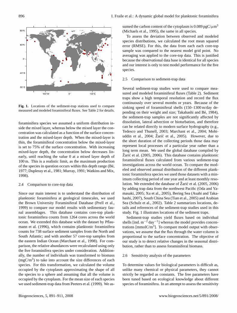
Fig. 1. Locations of the sediment-trap stations used to comparemeasured and modeled foraminiferal fluxes. See Table 2 for details.

foraminifera species we assumed a uniform distribution in-side the mixed layer, whereas below the mixed layer the con-centration was calculated as a function of the surface concen-tration and the mixed-layer depth. When the mixed-layer isthin, the foraminiferal concentration below the mixed-layeris set to 75% of the surface concentration. With increasingmixed-layer depth, the concentration below decreases lin-early, until reaching the value 0 at a mixed layer depth of100 m. This is a realistic limit, as the maximum productionof the species in question occurs within this depth range (Be,1977; Duplessy et al., 1981; Murray, 1991; Watkins and Mix,1998).

2.4 Comparison to core-top data

Since our main interest is to understand the distribution ofplanktonic foraminifera at geological timescales, we usedthe Brown University Foraminiferal Database (Prell et al.,1999) to compare our model results with sedimentary fau-nal assemblages. This database contains core-top plank-tonic foraminifera counts from 1264 cores across the worldocean. We extended this database with the dataset byPflau-mann et al.(1996), which contains planktonic foraminiferacounts for 738 surface sediment samples from the North andSouth Atlantic; and with another 57 core-top samples fromthe eastern Indian Ocean (Marchant et al., 1998). For com-parison, the relative abundances were recalculated using onlythe five foraminifera species under consideration. Addition-ally, the number of individuals was transformed to biomass(mgC/m3) to take into account the size differences of eachspecies. For this transformation, we calculated the volumeoccupied by the cytoplasm approximating the shape of allthe species to a sphere and assuming that all the volume isoccupied by the cytoplasm. For the mean size of each specieswe used sediment-trap data fromPeeters et al.(1999). We as-

sumed the carbon content of the cytoplasm is 0.089 pgC/µm3

(Michaels et al., 1995), the same in all species.To assess the deviation between observed and modeled

species distributions, we calculated the root mean squarederror (RMSE). For this, the data from each each core-topsample was compared to the nearest model grid point. Noaveraging was applied to the core-top data. This is justifiedbecause the observational data base is identical for all speciesand our interest is only to test model performance for the fivespecies.

2.5 Comparison to sediment-trap data

Several sediment-trap studies were used to compare mea-sured and modeled foraminiferal fluxes (Table 2). Sedimenttraps show a high temporal resolution and record the fluxcontinuously over several months or years. Because of thesinking speed of foraminiferal shells (150–1300 m/day de-pending on their weight and size;Takahashi and Be, 1984),the sediment-trap samples are not significantly affected bydissolution, lateral advection or bioturbation, and thereforecan be related directly to modern surface hydrography (e.g.,Tedesco and Thunell, 2003; Marchant et al., 2004; Mohi-uddin et al., 2004; Zaric et al., 2005). However, due tothe short duration of the collecting periods those data mayrepresent local processes of a particular year rather than along term mean. We used the global database compiled byZaric et al.(2005, 2006). This database contains planktonicforaminiferal fluxes calculated from various sediment-trapinvestigations across the world ocean. To compare the mod-eled and observed annual distribution of the different plank-tonic foraminifera species we used those datasets with a min-imum collecting period of one year and at least monthly reso-lution. We extended the database ofZaric et al.(2005, 2006)by adding trap data from the northwest Pacific (Oda and Ya-masaki, 2005; Xu et al., 2005), Bering Sea (Asahi and Taka-hashi, 2007), South China Sea (Tian et al., 2005) and ArabianSea (Schulz et al., 2002). Table 2 summarizes locations, de-tails and references of the sediment-trap studies used in thisstudy. Fig. 1 illustrates locations of the sediment traps.

Sediment-trap studies yield fluxes based on individualshells [ind. m−2 day−1] whereas the model provides concen-trations [mmolC/m3]. To compare model output with obser-vations, we assume that the flux through the water column isproportional to the surface concentration. The objective ofour study is to detect relative changes in the seasonal distri-bution, rather than to assess foraminiferal biomass.

2.6 Sensitivity analysis of the parameters

To determine values for biological parameters is difficult as,unlike many chemical or physical parameters, they cannotstrictly be regarded as constants. The free parameters havebeen tuned based on ecological knowledge about differentspecies of foraminifera. In an attempt to assess the sensitivity



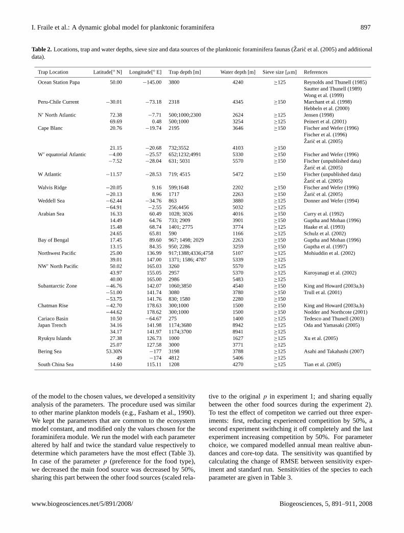
Table 2. Locations, trap and water depths, sieve size and data sources of the planktonic foraminifera faunas (Zaric et al.(2005) and additionaldata).

Trap Location Latitude[◦ N] Longitude[◦ E] Trap depth [m] Water depth [m] Sieve size [µm] References

Ocean Station Papa 50.00 −145.00 3800 4240 ≥125 Reynolds and Thunell (1985)Sautter and Thunell (1989)Wong et al. (1999)

Peru-Chile Current −30.01 −73.18 2318 4345 ≥150 Marchant et al. (1998)Hebbeln et al. (2000)

N’ North Atlantic 72.38 −7.71 500;1000;2300 2624 ≥125 Jensen (1998)69.69 0.48 500;1000 3254 ≥125 Peinert et al. (2001)

Cape Blanc 20.76 −19.74 2195 3646 ≥150 Fischer and Wefer (1996)Fischer et al. (1996)Zaric et al. (2005)

21.15 −20.68 732;3552 4103 ≥150W’ equatorial Atlantic −4.00 −25.57 652;1232;4991 5330 ≥150 Fischer and Wefer (1996)

−7.52 −28.04 631; 5031 5570 ≥150 Fischer (unpublished data)Zaric et al. (2005)

W Atlantic −11.57 −28.53 719; 4515 5472 ≥150 Fischer (unpublished data)Zaric et al. (2005)

Walvis Ridge −20.05 9.16 599;1648 2202 ≥150 Fischer and Wefer (1996)−20.13 8.96 1717 2263 ≥150 Zaric et al. (2005)

Weddell Sea −62.44 −34.76 863 3880 ≥125 Donner and Wefer (1994)−64.91 −2.55 256;4456 5032 ≥125

Arabian Sea 16.33 60.49 1028; 3026 4016 ≥150 Curry et al. (1992)14.49 64.76 733; 2909 3901 ≥150 Guptha and Mohan (1996)15.48 68.74 1401; 2775 3774 ≥125 Haake et al. (1993)24.65 65.81 590 1166 ≥125 Schulz et al. (2002)

Bay of Bengal 17.45 89.60 967; 1498; 2029 2263 ≥150 Guptha and Mohan (1996)13.15 84.35 950; 2286 3259 ≥150 Guptha et al. (1997)

Northwest Pacific 25.00 136.99 917;1388;4336;4758 5107 ≥125 Mohiuddin et al. (2002)39.01 147.00 1371; 1586; 4787 5339 ≥125

NW’ North Pacific 50.02 165.03 3260 5570 ≥12543.97 155.05 2957 5370 ≥125 Kuroyanagi et al. (2002)40.00 165.00 2986 5483 ≥125

Subantarctic Zone −46.76 142.07 1060;3850 4540 ≥150 King and Howard (2003a,b)−51.00 141.74 3080 3780 ≥150 Trull et al. (2001)−53.75 141.76 830; 1580 2280 ≥150

Chatman Rise −42.70 178.63 300;1000 1500 ≥150 King and Howard (2003a,b)−44.62 178.62 300;1000 1500 ≥150 Nodder and Northcote (2001)

Cariaco Basin 10.50 −64.67 275 1400 ≥125 Tedesco and Thunell (2003)Japan Trench 34.16 141.98 1174;3680 8942 ≥125 Oda and Yamasaki (2005)

34.17 141.97 1174;3700 8941 ≥125Ryukyu Islands 27.38 126.73 1000 1627 ≥125 Xu et al. (2005)

25.07 127.58 3000 3771 ≥125Bering Sea 53.30N −177 3198 3788 ≥125 Asahi and Takahashi (2007)

49 −174 4812 5406 ≥125South China Sea 14.60 115.11 1208 4270 ≥125 Tian et al. (2005)

of the model to the chosen values, we developed a sensitivityanalysis of the parameters. The procedure used was similarto other marine plankton models (e.g.,Fasham et al., 1990).We kept the parameters that are common to the ecosystemmodel constant, and modified only the values chosen for theforaminifera module. We run the model with each parameteraltered by half and twice the standard value respectively todetermine which parameters have the most effect (Table 3).In case of the parameterp (preference for the food type),we decreased the main food source was decreased by 50%,sharing this part between the other food sources (scaled rela-

tive to the originalp in experiment 1; and sharing equallybetween the other food sources during the experiment 2).To test the effect of competiton we carried out three exper-iments: first, reducing experienced competition by 50%, asecond experiment swithching it off completely and the lastexperiment increasing competition by 50%. For parameterchoice, we compared modelled annual mean realtive abun-dances and core-top data. The sensitivity was quantified bycalculating the change of RMSE between sensitivity exper-iment and standard run. Sensitivities of the species to eachparameter are given in Table 3.



Table 3. Sensitivity analysis to the parameter values: Reduction of parameter values and resulting change of RMSE between the model andcore-top relative abundances (RMSE sensitivity experiment minus RMSE standard run)

Experiment Parameter changeN. pachyderma(sin.) N. pachyderma(dex.) G.bulloides G.ruber(white) G. sacculifer

1 pmain (−50%) –0.3 4.6 –2.9 –4.7 0.6

2 pmain (−50%) –0.3 4.6 –2.9 –4.7 0.6

3 d (−50%) – 4.0 –0.2 –1.9 –0.7

4 d (−100%) – 4.6 0.8 6.4 1.9

5 d (+50%) – 3.4 –0.5 –5.3 0.7

6 Gmax (−50%) 2.9 3.6 –1.9 –5.6 –0.5

7 Gmax (+50%) –0.0 4.1 0.7 –6.2 0.6

8 σ (−50%) 1.1 2.1 4.1 –7.1 –1.0

9 σ (+50%) 7.4 5.2 –0.1 –4.0 1.3

Experiments:1=Reduction of main food preference,p(SP,D,ZO or DR), by 50%; sharing this part between the other food sources (scaled in relation tooriginalp)2=Reduction of main food preference,p(SP,D,ZO or DR), by 50%; sharing this part equally between the other food sources3=Reduction of experienced competition by 50%4=Suppression of competition5=Increase of experienced competition by 50% 6=Decrease of maximum grazing rate,Gmax by 50%7=Increase of maximum grazing rate,Gmax by 50%8=Decrease of temperature tolerance range,σ by 50%9=Increase of temperature tolerance range,σ by 50%

3 Results

3.1 Spatial distribution patterns

Modeled global distribution patterns of the five foraminiferaspecies are shown together with the corresponding core-topdata in Figs. 2–6. The model results are expressed as rela-tive abundances as derived from the biomass data. Relativeabundances for core-top data consider only the five speciesincluded in the model. The global distribution ofN. pachy-derma(sin.) shows the lowest RMSE, around 9%, while forthe remaining the species the error varies between 22% and25%.

N. pachyderma(sin.) is a cold-water species, and dom-inates planktonic foraminiferal assemblages in polar waters(Pflaumann et al., 1996; Bauch et al., 2003; Kucera et al.,2005). Previous work has shown that it can survive withinAntarctic sea ice (Dieckman et al., 1991; Spindler, 1996;Schnack-Schiel et al., 2001). It is usually used as a proxyfor cold water conditions (Bauch et al., 1997). Core-top,as well as modeled assemblages, show the highest relativeabundances (up to 100%) in polar waters (Fig. 2).

N. pachyderma(dex.) is typical of subpolar to transitionalwater masses. In the surface sediment samples,N. pachy-derma(dex.) shows a very high relative abundance in theNorth Atlantic Ocean, the Benguela upwelling system, partsof the Southern Ocean and in the equatorial upwelling of the

Pacific Ocean. It is also present, although at lower abun-dance, in the upwelling systems off northwest Africa. Themodel output shows very high concentrations in the Peru-Chile current and the eastern boundary upwelling systems,as well as south of Iceland, and moderate abundances at midlatitudes (Fig. 3).

Like N. pachyderma(dex.),G. bulloidestypically occursin subpolar and transitional water masses (Bradshaw, 1959;Tolderlund and Be, 1971; Be, 1977), and is also found in up-welling areas (Duplessy et al., 1981; Thunell and Reynolds,1984; Hemleben et al., 1989). Temperature does not seem tobe a controlling factor in the distribution of this species, al-though the exact relationship between environmental param-eters and geographical distribution ofG. bulloidesmay bemasked by the fact that this species group comprises severaldistinct genotypes (Darling et al., 1999, 2000; Stewart et al.,2001; Kucera and Darling, 2002; Darling et al., 2003). Gen-erally, the abundance ofG. bulloidesis related to high pro-ductivity areas (Prell and Curry, 1981; Be et al., 1985; Hem-leben et al., 1989; Giraudeau, 1993; Watkins and Mix, 1998;Zaric et al., 2005). G. bulloidesshows a high relative abun-dance in the surface sediment samples of the North AtlanticOcean, the upwelling systems off northwest and southwestAfrica, the Southern Ocean, the northern Indian Ocean, andto a lesser extent, the upwelling region off Baja California.The model results show high concentrations ofG. bulloidesin the subpolar waters of both hemispheres, in the eastern



Fig. 2. N. pachyderma(sin.) relative abundances (%) from core-top (left) foraminiferal assemblages (Pflaumann et al., 1996; Marchant etal., 1998; Prell et al., 1999) and model output (right). Relative abundances consider only the species included in the model. RMSE is 9%.

Fig. 3. N. pachyderma(dex.) relative abundances (%) from core-top (left) foraminiferal assemblages (Pflaumann et al., 1996; Marchant etal., 1998; Prell et al., 1999) and model output (right). Relative abundances consider only the species included in the model. RMSE is 22%.

boundary currents of the southern hemisphere and in somelocations of the Arabian Sea (Fig. 4).

The seafloor record shows high relative abundance ofG. ruber (white) in the central North and South Atlantic aswell as the South Pacific and less pronounced relative abun-dance in the South Indian Ocean up to 40◦ S. The model out-put shows a similar pattern with high relative abundances intropical and subtropical waters of the Atlantic, Pacific and In-dian Oceans, and very low relative abundances in upwellingareas (Fig. 5).

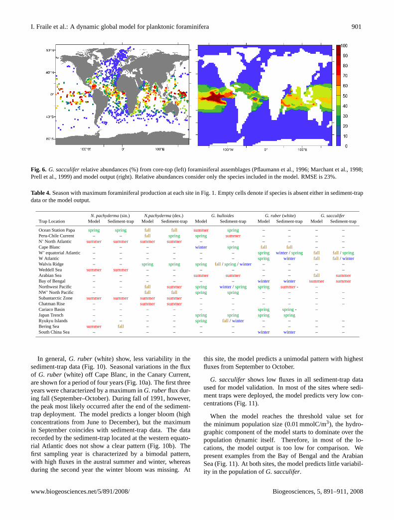
G. sacculifershows a clear preference for high tempera-tures (optimum of 28◦C) and is absent (or in concentrations≤10%) below 23◦C (Zaric et al., 2005). Core-top data showthis species is limited to tropical waters, reflecting its narrowtemperature tolerance (Fig. 6). The highest abundances occurin surface sediments from the equatorial Pacific and central

Indian Ocean. The relative abundance in most of the core-topdata from the upwelling region of the Arabian Sea is<10%.The annual mean distribution pattern ofG. sacculiferin themodel is limited to tropical waters, with highest concentra-tions in the equatorial Pacific. The model correctly simulatesabsence or low concentrations (<10%) in eastern upwellingsystems as well as in the upwelling area of the Arabian Sea.

3.2 Temporal distribution patterns

We used several sediment-trap datasets to assess the mod-eled seasonal variations in foraminifera abundance. We limitthe following comparison between the model output and thesediment-trap data to a few examples (Figs. 7–11).

In most of the cases, the sediment-trap data exhibit verypronounced interannual variability. In contrast, the model



Fig. 4. G. bulloidesrelative abundances (%) from core-top (left) foraminiferal assemblages (Pflaumann et al., 1996; Marchant et al., 1998;Prell et al., 1999) and model output (right). Relative abundances consider only the species included in the model. RMSE is 25%.

Fig. 5. G. ruber (white) relative abundances (%) from core-top (left) foraminiferal assemblages (Pflaumann et al., 1996; Marchant et al.,1998; Prell et al., 1999) and model output (right). Relative abundances consider only the species included in the model. RMSE is 25%.

is forced with climatological data (i.e., long-term averages),and is therefore unable to reproduce interannual variability.For that reason, we focused on the season with maximumproduction. In order to compare modeled and observed timeseries, we picked the season when maximum foraminiferalproduction occurs (Table 4). When sediment-trap were de-ployed for more than one year we considered the season inwhich most maxima occur.

Interannual variability ofN. pachyderma(sin.) in all thelocations is very high (Fig. 7), but the timing of the signalagrees between observed and predicted data.

The flux of N. pachyderma(dex.) increases during sum-mer (July–October) in northern North Atlantic (Fig. 8a).The seasonal pattern of predicted concentrations correspondswell with the trap record.

Sediment-trap data located at Subantarctic Zone show anincrease of theN. pachyderma(dex.) population during

the summer (January–February). In accordance with thesediment-trap data, the model results also show the highestconcentrations during the summer (Fig. 8b).

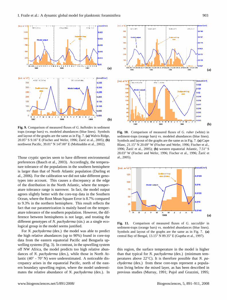
Examples forG. bulloidesare shown in Fig. 9.At Walvis Ridge, the sediment-trap data reveals a strong

seasonality, where maxima occurs in fall (September–November) and in spring (May–June). The model success-fully captures this bimodal pattern, with the main bloomoccurring in spring. The second example represents a sta-tion north of the Kuroshio current in the northwest Pa-cific (Fig. 9b). At this location the model predicts a smallpeak during winter (December–January) and the maximumduring early summer (May–June). The time-series recordalso presents this bimodal pattern; nevertheless, model andsediment-trap show better correspondence during the secondyear.



Fig. 6. G. sacculiferrelative abundances (%) from core-top (left) foraminiferal assemblages (Pflaumann et al., 1996; Marchant et al., 1998;Prell et al., 1999) and model output (right). Relative abundances consider only the species included in the model. RMSE is 23%.

Table 4. Season with maximum foraminiferal production at each site in Fig. 1. Empty cells denote if species is absent either in sediment-trapdata or the model output.

N. pachyderma(sin.) N.pachyderma(dex.) G. bulloides G. ruber(white) G. sacculiferTrap Location Model Sediment-trap Model Sediment-trap Model Sediment-trap Model Sediment-trap Model Sediment-trap

Ocean Station Papa spring spring fall fall summer spring – – – –Peru-Chile Current – – fall spring spring summer – – – –N’ North Atlantic summer summer summer summer – – – – – –Cape Blanc – – – – winter spring fall fall – –W’ equatorial Atlantic – – – – – – spring winter / spring fall fall / springW Atlantic – – – – – – spring winter fall fall / winterWalvis Ridge – – spring spring spring fall / spring/ winter – – – –Weddell Sea summer summer – – – – – – – –Arabian Sea – – – – summer summer – – fall summerBay of Bengal – – – – – – winter winter summer summerNorthwest Pacific – – fall summer spring winter / spring spring summer- –NW’ North Pacific – – fall fall spring spring – – – –Subantarctic Zone summer summer summer summer – – – – – –Chatman Rise – – summer summer – – – – – –Cariaco Basin – – – – – – spring spring- –Japan Trench – – – – spring spring spring springRyukyu Islands – – – – spring fall / winter – – – –Bering Sea summer fall – – – – – – – –South China Sea – – – – – – winter winter – –

In general,G. ruber (white) show, less variability in thesediment-trap data (Fig. 10). Seasonal variations in the fluxof G. ruber (white) off Cape Blanc, in the Canary Current,are shown for a period of four years (Fig. 10a). The first threeyears were characterized by a maximum inG. ruberflux dur-ing fall (September–October). During fall of 1991, however,the peak most likely occurred after the end of the sediment-trap deployment. The model predicts a longer bloom (highconcentrations from June to December), but the maximumin September coincides with sediment-trap data. The datarecorded by the sediment-trap located at the western equato-rial Atlantic does not show a clear pattern (Fig. 10b). Thefirst sampling year is characterized by a bimodal pattern,with high fluxes in the austral summer and winter, whereasduring the second year the winter bloom was missing. At

this site, the model predicts a unimodal pattern with highestfluxes from September to October.

G. sacculifershows low fluxes in all sediment-trap dataused for model validation. In most of the sites where sedi-ment traps were deployed, the model predicts very low con-centrations (Fig. 11).

When the model reaches the threshold value set forthe minimum population size (0.01 mmolC/m3), the hydro-graphic component of the model starts to dominate over thepopulation dynamic itself. Therefore, in most of the lo-cations, the model output is too low for comparison. Wepresent examples from the Bay of Bengal and the ArabianSea (Fig. 11). At both sites, the model predicts little variabil-ity in the population ofG. sacculifer.



(a)

(b)

Fig. 7. Comparison of measured fluxes ofN. pachyderma(sin.)in sediment traps (orange bars) vs. modeled abundances (bluelines). Note the difference in units between sediment-trap data[ind. m−2 day−1] and model output [mmolC/m3], which doesnot hamper with the assessment of the season of maximumforaminiferal production. Grey bars indicate gaps in sediment-trapdata.(a) Ocean Station PAPA, in northwest Pacific, 50◦ N 145◦ W(Reynolds and Thunell, 1985; Sautter and Thunell, 1989; Wonget al., 1999); (b) Weddell Sea, 64.91◦ S 2.55◦ W, in the SouthernOcean (Donner and Wefer, 1994).

3.3 Spatio-temporal distribution pattern

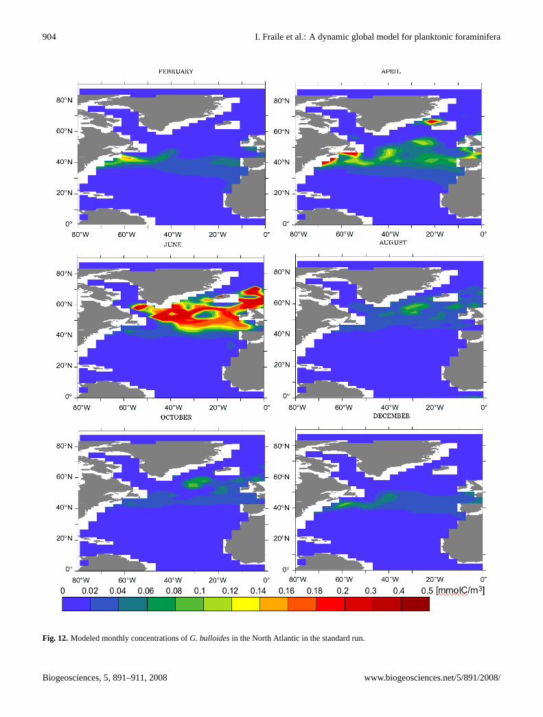
We analyzed the model prediction for the temporal varia-tion of G. bulloidesin the North Atlantic. Fig. 12 showsthe model output ofG. bulloidesconcentrations throughoutthe year in the North Atlantic. The maximum concentrationsoccur around 40◦ N during spring (March–April) and around60◦ N during summer (June–July), following the phytoplank-ton bloom in the model.

3.4 Sensitivity experiment: spatio-temporal distributionpatterns with constant temperature

We ran the foraminifera module with a constant tempera-ture of 12◦C everywhere to test the sensitivity ofG. bulloi-des to other environmental parameters (mainly food avail-ability). The chosen temperature corresponds to the optimaltemperature of this species in the model. Fig. 13 shows thespatio-temporal distribution ofG. bulloidesin the North At-lantic for this experimental run. In general, absolute concen-trations ofG. bulloidesare higher than in the standard run(Fig. 12). However, seasonal pattern does not change sub-stantially from the standard run: During spring the modelpredicts the highest concentrations in the southern region(around 40◦) while during summer, the bloom shifts to higherlatitudes.

(a)

(b)

Fig. 8. N. pachyderma(dex.) in sediment traps (orange bars)vs. modeled abundances (blue lines). Symbols and layout of thegraphs are the same as in Fig. 7.(a) northern North Atlantic,69.69◦ N 0.48◦ E (Jensen, 1998); (b) Subantarctic Zone, 46.76◦ S142.07◦ E (Trull et al., 2001; King and Howard, 2003a,b).

4 Discussion

4.1 Comparison with core-top data

In general, the global distribution patterns of foraminiferaspecies predicted by the model are very close to those ex-pected from core-top data.

The core-top data reflect the integrated flux through thewater column, while our model reflects the situation in themixed layer. As a consequence, some of the discrepanciesbetween model and core-top distributions could be due tothe different depth habitats of the species. However, the fivespecies simulated in our model live for most of their life cyclein the upper part of the water-column, thus we expect only asmall error at a global scale. In addition, fossil faunal assem-blages may be altered by selective dissolution (Berger, 1968;Thunell and Honjo, 1981; Le and Thunell, 1996; Dittert andHenrich, 1999), and by displacement through subsurface cur-rents or bioturbation processes (Be, 1977; Be and Hutson,1977; Boltovskoy, 1994). Since we can not take into accountany of these factors, these processes may explain some of thediscrepancies between core-top data and the model results.

The global distribution pattern ofN. pachyderma(sin.) isvery similar to that in the core-top data (Fig. 2). DistinctN. pachyderma(sin.) genotypes were identified byDarling etal. (2004) in the Arctic and Antarctic polar/subpolar waters.



(a)

(b)

Fig. 9. Comparison of measured fluxes ofG. bulloidesin sedimenttraps (orange bars) vs. modeled abundances (blue lines). Symbolsand layout of the graphs are the same as in Fig. 7.(a) Walvis Ridge,20.05◦ S 9.16◦ E (Fischer and Wefer, 1996; Zaric et al., 2005); (b)northwest Pacific, 39.01◦ N 147.00◦ E (Mohiuddin et al., 2002).

Those cryptic species seem to have different environmentalpreferences (Bauch et al., 2003). Accordingly, the tempera-ture tolerance of the populations in the southern hemisphereis larger than that of North Atlantic population (Darling etal., 2006). For the calibration we did not take different geno-types into account. This causes a discrepancy at the edgeof the distribution in the North Atlantic, where the temper-ature tolerance range is narrower. In fact, the model outputagrees slightly better with the core-top data in the SouthernOcean, where the Root Mean Square Error is 8.7% comparedto 9.3% in the northern hemisphere. This result reflects thefact that our parametrization is mainly based on the temper-ature tolerance of the southern population. However, the dif-ference between hemispheres is not large, and treating thedifferent genotypes ofN. pachyderma(sin.) as a single eco-logical group in the model seems justified.

For N. pachyderma(dex.) the model was able to predictthe high relative abundances (up to 90%) found in core-topdata from the eastern equatorial Pacific and Benguela up-welling systems (Fig. 3). In contrast, in the upwelling systemoff NW Africa, the model predicts too high relative abun-dances ofN. pachyderma(dex.), while those in North At-lantic (40◦ - 70◦ N) were underestimated. A noticeable dis-crepancy arises in the equatorial Pacific, north of the east-ern boundary upwelling region, where the model underesti-mates the relative abundance ofN. pachyderma(dex.). In

(a)

(b)

Fig. 10. Comparison of measured fluxes ofG. ruber (white) insediment-traps (orange bars) vs. modeled abundances (blue lines).Symbols and layout of the graphs are the same as in Fig. 7.(a) CapeBlanc, 21.15◦ N 20.69◦ W (Fischer and Wefer, 1996; Fischer et al.,1996; Zaric et al., 2005); (b) western equatorial Atlantic, 7.51◦ S28.03◦ W (Fischer and Wefer, 1996; Fischer et al., 1996; Zaric etal., 2005).

(a)

Fig. 11. Comparison of measured fluxes ofG. sacculifer insediment-traps (orange bars) vs. modeled abundances (blue lines).Symbols and layout of the graphs are the same as in Fig. 7.(a)central Bay of Bengal, 13.15◦ N 89.35◦ E (Guptha et al., 1997).

this region, the surface temperature in the model is higherthan that typical forN. pachyderma(dex.) (minimum tem-peratures above 22◦C). It is therefore possible thatN. pa-chyderma(dex.) from these core-tops represent a popula-tion living below the mixed layer, as has been described inprevious studies (Murray, 1991; Pujol and Grazzini, 1995;



Fig. 12. Modeled monthly concentrations ofG. bulloidesin the North Atlantic in the standard run.



Fig. 13. Modeled monthly concentrations ofG. bulloidesin an experiment with constant mixed layer temperature of 12◦C.



Kuroyanagi and Kawahata, 2004), or that they are expatri-ated specimens from the upwelling region.

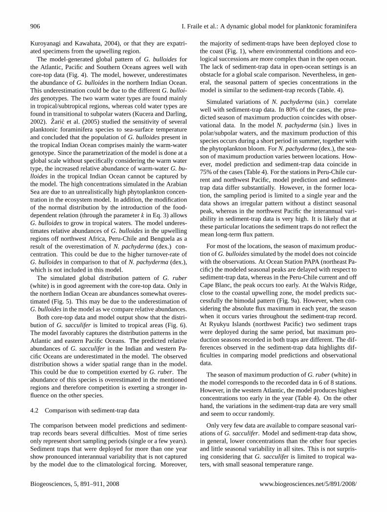
The model-generated global pattern ofG. bulloidesforthe Atlantic, Pacific and Southern Oceans agrees well withcore-top data (Fig. 4). The model, however, underestimatesthe abundance ofG. bulloidesin the northern Indian Ocean.This underestimation could be due to the differentG. bulloi-desgenotypes. The two warm water types are found mainlyin tropical/subtropical regions, whereas cold water types arefound in transitional to subpolar waters (Kucera and Darling,2002). Zaric et al.(2005) studied the sensitivity of severalplanktonic foraminifera species to sea-surface temperatureand concluded that the population ofG. bulloidespresent inthe tropical Indian Ocean comprises mainly the warm-watergenotype. Since the parametrization of the model is done at aglobal scale without specifically considering the warm watertype, the increased relative abundance of warm-waterG. bu-lloides in the tropical Indian Ocean cannot be captured bythe model. The high concentrations simulated in the ArabianSea are due to an unrealistically high phytoplankton concen-tration in the ecosystem model. In addition, the modificationof the normal distribution by the introduction of the food-dependent relation (through the parameterk in Eq. 3) allowsG. bulloidesto grow in tropical waters. The model underes-timates relative abundances ofG. bulloidesin the upwellingregions off northwest Africa, Peru-Chile and Benguela as aresult of the overestimation ofN. pachyderma(dex.) con-centration. This could be due to the higher turnover-rate ofG. bulloidesin comparison to that ofN. pachyderma(dex.),which is not included in this model.

The simulated global distribution pattern ofG. ruber(white) is in good agreement with the core-top data. Only inthe northern Indian Ocean are abundances somewhat overes-timated (Fig. 5). This may be due to the underestimation ofG. bulloidesin the model as we compare relative abundances.

Both core-top data and model output show that the distri-bution of G. sacculiferis limited to tropical areas (Fig. 6).The model favorably captures the distribution patterns in theAtlantic and eastern Pacific Oceans. The predicted relativeabundances ofG. sacculiferin the Indian and western Pa-cific Oceans are underestimated in the model. The observeddistribution shows a wider spatial range than in the model.This could be due to competition exerted byG. ruber. Theabundance of this species is overestimated in the mentionedregions and therefore competition is exerting a stronger in-fluence on the other species.

4.2 Comparison with sediment-trap data

The comparison between model predictions and sediment-trap records bears several difficulties. Most of time seriesonly represent short sampling periods (single or a few years).Sediment traps that were deployed for more than one yearshow pronounced interannual variability that is not capturedby the model due to the climatological forcing. Moreover,

the majority of sediment-traps have been deployed close tothe coast (Fig. 1), where environmental conditions and eco-logical successions are more complex than in the open ocean.The lack of sediment-trap data in open-ocean settings is anobstacle for a global scale comparison. Nevertheless, in gen-eral, the seasonal pattern of species concentrations in themodel is similar to the sediment-trap records (Table. 4).

Simulated variations ofN. pachyderma(sin.) correlatewell with sediment-trap data. In 80% of the cases, the prea-dicted season of maximum production coincides with obser-vational data. In the modelN. pachyderma(sin.) lives inpolar/subpolar waters, and the maximum production of thisspecies occurs during a short period in summer, together withthe phytoplankton bloom. ForN. pachyderma(dex.), the sea-son of maximum production varies between locations. How-ever, model prediction and sediment-trap data coincide in75% of the cases (Table 4). For the stations in Peru-Chile cur-rent and northwest Pacific, model prediction and sediment-trap data differ substantially. However, in the former loca-tion, the sampling period is limited to a single year and thedata shows an irregular pattern without a distinct seasonalpeak, whereas in the northwest Pacific the interannual vari-ability in sediment-trap data is very high. It is likely that atthese particular locations the sediment traps do not reflect themean long-term flux pattern.

For most of the locations, the season of maximum produc-tion of G. bulloidessimulated by the model does not coincidewith the observations. At Ocean Station PAPA (northeast Pa-cific) the modeled seasonal peaks are delayed with respect tosediment-trap data, whereas in the Peru-Chile current and offCape Blanc, the peak occurs too early. At the Walvis Ridge,close to the coastal upwelling zone, the model predicts suc-cessfully the bimodal pattern (Fig. 9a). However, when con-sidering the absolute flux maximum in each year, the seasonwhen it occurs varies throughout the sediment-trap record.At Ryukyu Islands (northwest Pacific) two sediment trapswere deployed during the same period, but maximum pro-duction seasons recorded in both traps are different. The dif-ferences observed in the sediment-trap data highlights dif-ficulties in comparing model predictions and observationaldata.

The season of maximum production ofG. ruber(white) inthe model corresponds to the recorded data in 6 of 8 stations.However, in the western Atlantic, the model produces highestconcentrations too early in the year (Table 4). On the otherhand, the variations in the sediment-trap data are very smalland seem to occur randomly.

Only very few data are available to compare seasonal vari-ations ofG. sacculifer. Model and sediment-trap data show,in general, lower concentrations than the other four speciesand little seasonal variability in all sites. This is not surpris-ing considering thatG. sacculifer is limited to tropical wa-ters, with small seasonal temperature range.



4.3 Sensitivity analysis

In an attempt to assess the sensitivity of the model to thechosen parameter values, we performed a sensitivity anal-ysis of the parameters. The procedure used was similar toother marine plankton models (e.g.,Fasham et al., 1990).We kept the parameters that are common to the ecosystemmodel constant, and modified only the values chosen for theforaminifera module. We run the model with each parameteraltered by half and twice the standard value respectively todetermine which parameters have the most effect (Table 3).

The sensitivity was quantified by calculating the change ofRMSE between the sensitivity experiment and the standardrun. The results (Table 3) indicate that none of the param-eters lead to uniform changes for all species. The modelseems to be more robust forG. sacculifer than for otherspecies. In several experiments, the error between model andcore-top data decreases. This occurs because the standardparametrization is based on ecological data compiled fromliterature rather than ”tuned” to obtain a better fit. Remov-ing competition generates a general increase of RMSE. Notsurprisingly, the temperature tolerance range (σ ) seems to bethe most sensitive parameter.

4.4 Model experiment with constant mixed-layer tempera-ture

When the foraminifera model is run with a constant tem-perature of 12◦C, G. bulloides in the North Atlantic stillshowed highest concentrations at low latitudes during springand maximum concentrations at higher latitudes in June,linked to the seasonal migration of the phytoplankton bloom(Fig. 13). This indicates that temperature is not the only con-trolling factor, but that food supply plays an important role inthe temporal distribution pattern of this species. The experi-ment confirms the results ofGanssen and Kroon(2000), whofrom isotopic studies on North Atlantic surface sediments,concluded thatG. bulloidesreflects temperatures of a north-ward migrating spring bloom.

5 Summary and conclusions

A global model has been developed that predicts monthlyplanktonic foraminifera concentrations forN. pachyderma(sin.), N. pachyderma(dex.),G. bulloides, G. ruber (white)and G. sacculifer. It is a nonlinear dynamic model simu-lating growth rate of foraminifera populations using infor-mation from an underlying ecosystem model (Moore et al.,2002a).

The model aims at predicting the distribution of planktonicforaminifera at geological timescales. Overall, the globaldistribution patterns of the predicted species are similar tocore-top data.

Modeled seasonal variations overall agree with sediment-trap records for most of the locations, although the compar-

ison is hampered by interannual variability not captured bythe model.

A sensitivity experiment using a constant temperature of12◦C indicates that food availability (primary production inthe case ofG. bulloides) is an important factor controllingthe distribution of some species.

Our model provides a tool that will contribute to better as-sessing how changing environmental conditions in the geo-logical past affected the distribution of foraminifera in spaceand time.

Quantitative data and a better knowledge of ecologicalprocess from laboratory and field studies are essential for fur-ther improvement of the current model. Results may also beimproved by including additional information, such as differ-ent classes of zooplankton, or by explicitly resolving depth.

Acknowledgements.We appreciate the contributions and helpfulcomments of R. Schiebel, M. Peck, A. Beck, A. Bisset, and 4referees who improved the manuscript. Thanks also to M. Prangeand T. Laepple for analytical assistance and G. Fischer forproviding sediment-trap data. Special thanks to A. Manschkefor computer support. This project was supported by the DFG(Deutsche Forschungsgemeinschaft) as part of the EuropeanGraduate Collegue “Proxies in Earth History” (EUROPROX).

Edited by: C. Heinze

References

Anderson, O. R., Spindler, M., Be, A. W. H., and Hemleben, C.:Trophic activity of planktonic foraminifera, J. Mar. Biol. Assoc.U.K., 59, 791–799, 1979.

Arnold, A. J. and Parker, W. C.: Biogeography of planktonicForaminifera, in: Modern Foraminifera, edited by: Gupta,B. S. K., Dortrecht, Boston, London, 103–122, 1999.

Asahi, H. and Takahashi, K.: A 9-year time-series of plank-tonic foraminifer fluxes and environmental change in the Beringsea and the central subarctic Pacific Ocean, 1990–1999, Prog.Oceanogr., 72, 343–363, 2007.

Bauch, D., Carstens, J., and Wefer, G.: Oxygen isotope composi-tion of living Neogloboquadrina pachyderma(sin.) in the ArcticOcean, Earth. Planet. Sc. Lett., 146, 47–58, 1997.

Bauch, D., Darling, K., Simstich, J., Bauch, H. A., Erlenkeuser, H.and Kroon, D.: Palaeoceanographic implications of genetic vari-ation in living North AtlanticNeogloboquadrina pachyderma,Nature, 424, 299–302, 2003.

Be, A. W. H. and Hamilton, W. H.: Ecology of Recent planktonicforaminifera, Micropal., 13, 87–106, 1967.

Be, A. W. H. and Tolderlund, D. S.: Distribution and ecology of liv-ing planktonic foraminifera in surface waters of the Atlantic andIndian Oceans, in The Micropalaeontology of Oceans, edited by:Funnell, B. M. and Riedel, W. R., 105–149, Cambridge Univer-sity Press, 1967.

Be, A. W. H.: An ecological, zoogeographic and taxonomic reviewof recent planktonic foraminifera, in: Oceanic Micropalaeontol-ogy, edited by: Ramsay, A. T. S., 1–100, Academic Press Inc.,London, 1977.



Be, A. W. H. and Hutson, W. H.: Ecology of planktonicforaminifera and biogeographic patterns of life and fossil assem-blages in the Indian Ocean, Micropal., 23, 369–414, 1977.

Be, A. W. H., Caron, D. A., and Anderson, O. R.: Effects of feedingfrequency on life processes of the planktonic foraminiferGlo-bigerinoides sacculiferin laboratory culture, J. Mar. Biol. Assoc.U.K., 61, 257–277, 1981.

Be, A. W. H., Bishop, J. K. B., Sverdlove, M. S., and Gardner,W. D.: Standing stock, vertical distribution and flux of planktonicForaminifera in the Panama Basin, Mar. Micropal., 9, 307–333,1985.

Berger, W. H.: Planktonic foraminifera: selective solution and pa-leoclimatic interpretation, Deep-Sea Res., 15, 31–43, 1968.

Bijma, J., Faber, W. W. J., and Hemleben, C.: Temperatureand salinity limits for growth and survival of some planktonicforaminifers in laboratory cultures, J. Foramin. Res., 20, 95–116,1990.

Bishop, J. K. B. and Rossow, W. B.: Spatial and temporal variabilityof global surface solar irradiance, J. Geophys. Res., 96, 16 839–16 858, 1991.

Boltovskoy, D.: The sedimentary record of pelagic biogeography,Prog. Oceanogr., 34, 135–160, 1994.

Bradshaw, J. S.: Ecology of living planktonic foraminifera in theNorth and equatorial Pacific Ocean, Cushman Foundation forForaminiferal Research Contribution, 10, 25–64, 1959.

Caron, D. A., Be, A. W. H. and Anderson, O. R.: Effects onvariations in light intensity on life processes of the planktonicforaminifera Globigerinoides sacculifer in laboratory culture, J.Mar. Biol. Assoc. UK, 67, 323–341, 1981.

Caron, D. A. and Be, A. W. H.: Predicted and observed feeding ratesof the spinose planktonic foraminiferGlobigerinoides sacculifer,B. Mar. Sci., 35, 1–10, 1984.

Cavalieri, D., Gloerson, P., and Zwally, J.: DMSP SSM/I daily polargridded sea ice concentrations, October 1998 to September 1999,edited by: Maslanik, J. and Stroeve, J., National Snow and IceData Center, Boulder, CO, Digital media, 1990.

CLIMAP Project Members: The surface of the ice-age earth, Sci-ence, 191, 1131–1137, 1976.

Conan, S. M. H., and Brummer, G. J. A.:Fluxes of plankticforaminifera in response to monsoonal upwelling on the SomaliaBasin margin, Deep-Sea Res. II, 47, 2207–2227, 2000.

Conkright, M., Levitus, S., OBrien, T., Boyer T., Antonov, J. andStephens: World Ocean Atlas 1998 CD-ROM Data Set Docu-mentation, Tech. Rep. 15, NODC Internal Report, Silver Spring,MD, 16 pp., 1998.

Cullen, J. L.: Microfossil evidence for changing salinity patternsin the Bay of Bengal over the last 20,000 years, Palaeogeogr.Palaeocl., 35, 315–356, 1981.

Curry, W. B., Ostermann, D. R., Guptha, M. V. S., and Ittekkot, V.:Foraminiferal production and monsoonal upwelling in the Ara-bian Sea: evidence from sediment traps, in: Upwelling Systems:Evolution Since the Early Miocene, edited by: Summerhayes,C. P., Prell, W. L., and Emeis, K. C., 93–106, The GeologicalSociety, London, 1992.

Darling, K. F., Wade, C. M., Kroon, D., Leigh Brown, A. J., andBijma, J.: The diversity and distribution of modern planktonicforaminiferal small subunit ribosomal RNA genotypes and theirpotential as tracers of present and past ocean circulations, Paleo-ceanography, 14, 3–12, 1999.

Darling, K. F., Wade, C. M., Stewart, I. A., Kroon, D., Dingle, R.,and Leigh Brown, A. J.: Molecular evidence for genetic mix-ing of Arctic and Antarctic subpolar populations of planktonicforaminifers, Nature, 405, 43–47, 2000.

Darling, K. F., Kucera, M., Wade, C. M., von Langen, P., andPak, D.: Seasonal distribution of genetic types of planktonicforaminifer morphospecies in the Santa Barbara Channel andits paleoceanographic implications, Paleoceanography, 18, 1032,doi:10.1029/2001PA000723, 2003.

Darling, K. F.,Kucera, M., Pudsey, C. J. and Wade, C. M.: Molec-ular evidence links cryptic diversification in polar plankton toQuaternary climate dynamics, Proc. Natl. Acad. Sci., U. S. A.,101, 7657-7662, 2004.

Darling, K. F., Kucera, M., Kroon, D., and Wade, C. M.: Aresolution for the coiling direction paradox inNeoglobo-quadrina pachyderma, Paleoceanography, 21, 2011,doi:10.1029/2005PA001189, 2006.

Deuser, W. G. and Ross, E. H.: Seasonally abundant planktonicforaminifera of the Sargasso Sea: succession, deep-water fluxes,isotopic compositions, and paleoceanographic implications, J.Foramin. Res., 19, 268–293, 1989.

Dieckmann, G. S., Spindler, M., Lange, M. A., Ackley, S. F.,and Eicken, H.: Antarctic sea ice: a habitat for the foraminiferNeogloboquadrina pachyderma, J. Foramin. Res., 21, 182–189,1991.

Dittert, N. and Henrich, R.: Carbonate dissolution in the South At-lantic Ocean: evidence from ultrastructure breakdown inGlo-bigerina bulloides, Deep-Sea Res. I, 47, 603–620, 1999.

Donner, B. and Wefer, G.: Flux and stable isotope composi-tion of Neogloboquadrina pachydermaand other planktonicforaminifers in the Southern Ocean (Atlantic sector), Deep-SeaRes. I, 41, 1733–1743, 1994.

Duplessy, J. C., Delibrias, G., Turon, J. L., Pujol, C., and Duprat, J.:Deglacial warming of the Northeastern Atlantic Ocean: correla-tion with the paleoclimatic evolution of the European continent,Palaeogeogr. Palaeocl., 35, 121–144, 1981.

Edwards, A. M. and Yool, A.: The role of higher predation in plank-ton population models, J. Plankton Res., 22, 1085–1112, 2000.

Eguchi, N. O., Kawahata, H., and Taira, A.: Seasonal Response ofPlanktonic Foraminifera to Surface Ocean Condition: SedimentTrap Results from the Central North Pacific Ocean, J. Oceanogr.,55, 681–691, 1999.

Fasham, M. J. R., Ducklow, H. W. and McKelvie, S. M.: Anitrogen-based model of plankton dynamics in the oceanic mixedlayer, J. Mar. Res., 48, 591–639, 1990.

Fischer, G. and Wefer, G.: Long-term Observation of ParticleFluxes in the Eastern Atlantic: Seasonality, Changes of Flux withDepth and Comparison with the Sediment Record, in: The SouthAtlantic: Present and Past Circulation, edited by: Wefer, G.,Berger, W. H., Siedler, G., and Webb, D. J., 325–344, Springer-Verlag, Berlin Heidelberg, 1996.

Fischer, G., Donner, B., Ratmeyer, V., Davenport, R., and Wefer,G.: Distinct year-to-year particle flux variations off Cape Blancduring 1988–1991: Relation toδ18O-deduced sea-surface tem-peratures and trade winds, J. Mar. Res., 54, 73–98, 1996.

Ganssen, G. M. and Kroon, D.: The isotopic signature of planktonicforaminifera from NE Atlantic surface sediments: implicationsfor the reconstruction of past oceanic conditions, J. Geol. Soc.,157, 693–699, 2000.



Gastrich, M. D.: Ultrastructure of a new intracellular symbiotic algafound within planktonic foraminifera, J. Phycol., 23, 623–632,1987.

Gent, P. R., Bryan, F. O., Danabasoglu, G., Doney, S. C., Holland,W. R., Large, W. G., and McWilliams, J. C.: The NCAR climatesystem model global ocean component, J. Climate, 11, 1287–1306, 1998.

Giraudeau, J.: Planktonic foraminiferal assemblages in surface sed-iments from the southwest African continental margin, Mar.Geol., 110, 47–62, 1993.

Guptha, M. V. S. and Mohan, R.: Seasonal variability of the verti-cal fluxes ofGlobigerina bulloides(d Orbigny) in the northernIndian Ocean, Mitt. Geol.-Palaont. Inst. Univ. Hamburg, 79, 1–17, 1996.

Guptha, M. V. S., Curry, W. B., Ittekkot, V., and Muralinath, A. S.:Seasonal variation in the flux of planktic foraminifera: Sedimenttrap results from the Bay of Bengal, northern Indian Ocean, J.Foramin. Res., 27, 5–19, 1997.

Haake, B., Ittekkot, V., Rixen, T., Ramaswamy, V., Nair, R. R., andCurry, W. B.: Seasonality and interannual variability of particlefluxes to the deep Arabian Sea, Deep-Sea Res. I, 40, 1323–1344,1993.

Hebbeln, D., Marchant, M., and Wefer, G.: Seasonal variations ofthe particle flux in the Peru-Chile current at 30◦ S under normaland El Nino conditions, Deep-Sea Res. II, 47, 2101–2128, 2000.

Hemleben, C., Spindler, M., Breitinger, J., and Deuser, W. G.: Fieldand laboratory studies of the ontogeny and ecology ofGloboro-talia truncatulinoidesand G. hirsuta in the Sargasso Sea, J.Foramin. Res., 15, 254–272, 1985.

Hemleben, C., Spindler, M., and Anderson, O. R.: Modern Plank-tonic Foraminifera, Springer-Verlag, New York, 1989.

Jensen, S.: Planktische Foraminiferen im Europaischen Nordmeer:Verbreitung und Vertikalfluss sowie ihre Entwicklung wahrendder letzten 15000 Jahre, Berichte SFB 313, Univ. Kiel, 75, 105pp., 1998.

Kiefer, T.: Produtivitat und Temperaturen im subtropischen Nordat-lantik: zyklische und abrupte Veranderungen im spaten Quartar,Berichte – Reports, Geol.-Palaont. Inst., Univ. Kiel, 90, 1–127,1998.

King, A. L. and Howard, W. R.: Seasonality of foraminiferal flux insediment traps at Chatham Rise, SW Pacific: implications forpaleotemperature estimates, Deep-Sea Res. I, 48, 1687–1708,2001.

King, A. L. and Howard, W. R.: Planktonic foraminiferalflux seasonality in Subantarctic sediment traps: A test forpaleoclimate reconstructions, Paleoceanography, 18, 1019,doi:1010.1029/2002PA000839, 2003a.

King, A. L. and Howard, W. R.: Seasonal Subantarctic PlanktonicForaminiferal Flux Data, available from the IGBP PAGES/WorldData Center for Paleoclimatology (http://www.ngdc.noaa.gov/paleo), Data Contribution Series # 2003-022., NOAA/NGDC Pa-leoclimatology Program, Boulder CO, 2003b.

Kucera, M. and Darling, K. F.: Cryptic species of planktonicforaminifera: their effect on paleoceanographic reconstructions,Philos. Tr. Roy. Soc. A, 360, 695–718, 2002.

Kucera, M., Rosell-Mele, A., Schneider, R., Waelbroeck, C., andWeinelt, M.: Reconstruction 15 of sea-surface temperatures fromassemblages of planktonic foraminifera: multi-technique ap-proach based on geographically constrained calibration data sets

and its application to glacial Atlantic and Pacific Oceans, Quat.Sci. Rev., 24, 951998, 2005.

Kuroyanagi, A., Kawahata, H., Nishi, H., and Honda, M. C.: Sea-sonal changes in planktonic foraminifera in the northwesternNorth Pacific Ocean: sediment trap experiments from subarcticand subtropical gyres, Deep-Sea Res. II, 49, 5627–5645, 2002.

Kuroyanagi, A. and Kawahata, H.: Vertical distribution of livingplanktonic foraminifera in the seas around Japan, Mar. Micropal.,53, 173–196, 2004.

Le, J. and Thunell, R. C.: Modelling planktic foraminiferal assem-blage changes and application to sea surface temperature estima-tion in the western equatorial Pacific Ocean, Mar. Micropal., 28,211–229, 1996.

Lea, D. W.: Trace elements in foraminiferal calcite, in: Modernforaminifera, edited by: Gupta, B. S. K., Dortrecht, Boston, Lon-don, 259–277, 1999.

Lee, J. J., McEnery, M. E., Pierce, S., Freudenthal, H. D.,and Muller, W. A.: Tracer experiments in feeding littoralforaminifera, J. Protozool., 13, 659–670, 1966.

Malmgren, B. A., Kucera, M., Nyberg, J., and Waelbroeck, C.:Comparison of statistical and artificial neural network tech-niques for estimating past sea surface temperature from plank-tonic foraminifer census data, Paleoceanography, 16, 520–530,2001.

Marchant, M., Hebbeln, D., and Wefer, G.: Seasonal flux patterns ofplanktic foraminifera in the Peru-Chile Current, Deep-Sea Res.I, 45, 1161–1185, 1998.

Marchant, M., Hebbeln, D., Giglio, S., Coloma C., and Gonzalez,H.: Seasonal and interannual variability in the flux of plankticforaminifers in the southern Humboldt Current System off cen-tral Chile, Deep-Sea Res. II, 51, 2441–2455, 2004.

Martinez, J. I., Taylor, L., Deckker, P., and Barrows, T.: Planktonicforaminifera from the eastern Indian Ocean: distribution andecology in relation to the Western Pacific Warm Pool (WPWP),Mar. Micropal., 34, 121–151, 1998.

Michaels, A. F., Caron, D. A., Swanberg, N. R., and Howse, F. A.:Planktonic sarcodines (Acantharia, Radiolaria, Foraminifera) insurface waters near Bermuda: abundance, biomass and verticalflux, J. Plankton Res., 17, 131–163, 1995.

Mohiuddin, M. M., Nishimura, A., Tanaka, Y., and Shimamoto, A.:Regional and interannual productivity of biogenic componentsand planktonic foraminiferal fluxes in the northwestern PacificBasin, Mar. Micropal., 45, 57–82, 2002.

Mohiuddin, M. M., Nishimura, A., Tanaka, Y., and Shimamoto,A.: Seasonality of biogenic particle and planktonic foraminiferafluxes: response to hydrographic variability in the Kuroshio Ex-tension, northwestern Pacific Ocean, Deep-Sea Res. I, 51, 1659–1683, 2004.

Monterey, G. and Levitus, S.: Seasonal variability ofmixed layerdepth for the world ocean, NOAA Atlas NESDIS 14, US Gov-ernment Printing Office, Washington, D.C., 1997.

Moore, J. K., Doney, S. C., Kleypas, J. A., Glover, D. M., and Fung,I. Y.: An intermediate complexity marine ecosystem model forthe global domain, Deep-Sea Res. II, 49, 403–462, 2002a.

Moore, J. K., Doney, S. C., Glover, D. M., and Fung, I. Y.: Ironcycling and nutrient-limitation patterns in surface waters oftheWorld Ocean, Deep-Sea Res. II, 49, 463–507, 2002b.

Morey, A. E., Mix, A. C., and Pisias, N. G.: Planktonicforaminiferal assemblages preserved in surface sediments cor-


http://www.ngdc.noaa.gov/paleo

http://www.ngdc.noaa.gov/paleo


respond to multiple environment variables, Quat. Sci. Rev., 24,925–950, 2005.

Mulitza, S., Durkoop, A., Hale, W., Wefer, G., and Niebler, H. S.:Planktonic foraminiferaa as recorders of past surface-water strat-ification, Geology, 25, 335–338, 1997.

Mulitza, S., Wolff, T., Patzold, J., Hale, W., and Wefer, G.: Temper-ature sensitivity of planktic foraminifera and its influence on theoxygen isotope record, Mar. Micropal., 33, 223–240, 1998.

Murray, J. W.: Ecology, and distribution of planktonic foraminifera,in: Biology of foraminfera, edited by: Lee, J. J. and Anderson,O. R., Academic Press, Harcourt, 255–284, 1991.

Niebler, H. S., Arz, H. W., Donner, B., Mulitza, S., Patzold, J., andWefer, G.: Sea surface temperatures in the equatorial and SouthAtlantic Ocean during the last glacial maximum (23–19 ka), Pa-leoceanography, 18, 1069, doi:1010.1029/2003PA000902, 2003.

Nodder, S. D. and Northcote, L. C.: Episodic particulate fluxes atsouthern temperate mid-latitudes (42–45◦ S) in the SubtropicalFront region, east of New Zealand, Deep-Sea Res. I, 48, 833–864, 2001.

Oda, M. and Yamasaki, M.: Sediment trap results from the JapanTrench in the Kuroshio domain: seasonal variations in the plank-tic foraminiferal flux, J. Foramin. Res., 35, 315–326, 2005.

Ortiz, J. D., Mix, A. C., and Collier, R. W.: Environmental controlof living symbiotic and asymbiotic foraminifera of the CaliforniaCurrent, Paleoceanography, 10, 987–1009, 1995.

Pearson, P. N. and Palmer, M. R.: Atmospheric carbon dioxide con-centrations over the past 60 million years, Nature, 406, 695–699,2000.

Peeters, F., Ivanova, E., Conan, S., Brummer, G. J., Ganssen, G.,Troelstra, S., and van Hinte, J.: A size analysis of plankticforaminifera from the Arabian Sea, Mar. Micropal., 36, 31–63,1999.

Peinert, R., Antia, A. N., Bauerfeind, E., Haupt, O., Krumbholz,M., Peeken, I., Bodungen, B. V., Ramseier, R., Voss, M., andZeitzschel, B.: Particle Flux Variability in the Polar and AtlanticBiogeochemical Provinces of the Nordic Seas, in: The NorthernNorth Atlantic: A Changing Environment, edited by: Schafer,P., Ritzrau, W., Schluter, M., and Thiede, J., 53–68, Springer,Berlin, 2001.

Pflaumann, U., Duprat, J., Pujol, C., and Labeyrie, L. D.: SIM-MAX: A modern analog technique to deduce Atlantic sea sur-face temperatures from planktonic foraminifera is deep-sea sedi-ments, Paleoceanography, 11, 15–35, 1996.

Pflaumann, U., Sarnthein, M., Chapman, M., d’Abreu, L., Fun-nell, B., Huels, M., Kiefer, T., Maslin, M., Schulz, H., Swal-low, J., van Kreveld, S., Vautravers, M., Vogelsang, E., andWeinelt, M.: Glacial North Atlantic: Sea-surface conditions re-constructed by GLAMAP 2000, Paleoceanography, 18, 1065,doi:1010.1029/2002PA000774, 2003.

Prell, W. L. and Curry, W. B.: Faunal and isotopic indices of mon-soonal upwelling: Western Arabian Sea, Oceanologica Acta, 4,91–95, 1981.

Prell, W. L., Martin, A., Cullen, J., and Trend, M.: The BrownUniversity Foraminiferal Data Base, IGBP PAGES/World DataCenter-A for Paleoclimatology, Data Contribution Series # 1999-027, NOAA/NGDC Paleoclimatology Program, Boulder CO,USA, 1999.

Pujol, C. and Grazzini, C. V.: Distribution patterns of live plankticforaminifers as related to regional hydrography and productive

systems of the Mediterranean Sea, Mar. Micropal., 25, 187–217,1995.

Reynolds, L. and Thunell, R. C.: Seasonal succession of planktonicforaminifera in the subpolar North Pacific, J. Foramin. Res., 15,282–301, 1985.

Rohling, E. J. and Cooke, S.: Stable oxygen and carbon isotopesin foraminiferal carbonate shells in: Modern foraminifera, editedby: Gupta, B. S. K., Dortrecht, Boston, London, 239–258, 1999.

Rossow, W. B. and Schiffer, R. A.: ISCCP cloud data products, B.Am. Meteorol. Soc., 72, 2–20, 1991.

Sautter, L. R. and Thunell, R. C.: Seasonal succession of planktonicforaminifera: results from a four-year time-series sediment trapexperiment in the northeast Pacific, J. Foramin. Res., 19, 253–267, 1989.

Schiebel, R., Hiller, B., and Hemleben, C.: Impacts of storms onrecent planktic foraminiferal test production and CaCO3 flux inthe North Atlantic at 47.8◦ N, 20.8◦ W (JGOFS), Mar. Micropal.,26, 115–129, 1995.

Schiebel, R., Bijma, J., and Hemleben, C.: Population dynamics ofthe planktic foraminiferGlobigerina bulloidesfrom the easternNorth Atlantic, Deep-Sea Res. 44, 1701–1713, 1997.

Schiebel, R., Waniek, J., Bork, M., and Hemleben, C.: Plankticforaminiferal production stimulated by chlorophyll redistribu-tion and entrainment of nutrients, Deep-Sea Res. I, 48, 721–740,2001.

Schnack-Schiel, S. B., Dieckmann, G. S., Gradinger, R., Melnikov,I. A., Spindler, M., and Thomas, D. N.: Meiofauna in sea ice ofthe Weddell Sea (Antarctica), Polar Biol., 24, 724–728, 2001.

Schulz, H., Von Rad, U., and Ittekkot, V.: Planktic foraminifera,particle flux and oceanic productivity off Pakistan, NE Ara-bian Sea: modern analogues and application to the paleoclimaticrecord, in: The Tectonic and Climatic Evolution of the ArabianSea Region, edited by: Clift, P. D., Kroon, D., Gaedicke, C., andCraig, J., Geol. Soc. Spec. Publ., 195, 499–516, 2002.

Spindler, M., Hemleben, C., Salomons, J. B., and Smit, L. P.: Feed-ing behavior of some planktonic foraminifers in laboratory cul-tures, J. Foramin. Res., 14, 237–249, 1984.

Spindler, M. and Dieckmann, G. S.: Distribution and Abundanceof the Planktic ForaminiferNeogloboquadrina pachydermainSea Ice of the Weddell Sea (Antarctica), Polar Biol., 5, 185–191,1986.

Spindler, M.: On the salinity tolerance of the planktonic foraminiferNeogloboquadrina pachydermafrom Antarctic sea ice, PolarBiol., 9, 85–91, 1996.

Steele, J. H. and Henderson, E. W.: The role of predation in plank-ton models, J. Plankton Res., 14, 157–172, 1992.

Stewart, I. A., Darling, K. F., Kroon, D., Wade, C. M., and Troel-stra, S. R.: Genotypic variability in subarctic Atlantic plankticforaminifera, Mar. Micropal., 43, 143–153, 2001.

Takahashi, K. and Be, A. W. H.: Planktonic foraminifera: factorscontrolling sinking speed, Deep-Sea Res., 31, 1477–1500, 1984.

Tedesco, K. A. and Thunell, R. C.: Seasonal and interannual vari-ations in planktonic foraminiferal flux and assemblage composi-tion in the Cariaco Basin, Venezuela, J. Foramin. Res., 33, 192–210, 2003.

Tegen, I. and Fung, I. Y.: Modeling of mineral dust in the atmo-sphere: sources, transport, and optical thickness, J. Geophys.Res., 99, 22 897–22 914, 1994.

Tegen, I. and Fung, I. Y.: Contribution to the atmospheric mineral



aerosol load from land surface modification, J. Geophys. Res.,100, 18 707–18 726, 1995.

Thunell, R. C. and Honjo, S.: Calcite dissolution and the modifica-tion of planktonic foraminiferal assemblages, Mar. Micropal., 6,169–182, 1981.

Thunell, R. C. and Reynolds, L. A.: Sedimentation of planktonicforaminifera: seasonal changes in species flux in the PanamaBasin, Micropaleontology, 30, 243–262, 1984.

Tian, J., Wang, P., Chen, R., and Cheng, X.: Quaternary upperocean thermal gradient variations in the South China Sea: Impli-cations for east Asian monsoon climate, Paleoceanography, 20,4007, doi:10.1029/2004PA001115, 2005.

Tolderlund, D. S. and Be, A. W. H.: Seasonal distribution of plank-tonic Foraminfera in the western North Atlantic, Micropalaeon-tology, 17, 297–329, 1971.

Trull, T. W., Bray, S. G., Manganini, S. J., Honjo, S., and Francois,R.: Moored sediment trap measurements of carbon export inthe Subantarctic and Polar Frontal Zones of the Southern Ocean,south of Australia, J. Geophys. Res., 106, 31 489–31 510, 2001.

Waelbroeck, C., Mulitza, S., Spero, H., Dokken, T., Kiefer, T., andCortijo, E.: A global compilation of late Holocene planktonicforaminiferalδ18O: relationship between surface water tempera-ture andδ18O, Quat. Sci. Rev., 24, 853–868, 2005.

Watkins, J. M., Mix, A. C., and Wilson, J.: Living plankticforaminifera: tracers of circulation and productivity regimes inthe central equatorial Pacific, Deep-Sea Res. II, 43, 1257–1282,1996.

Watkins, J. M. and Mix, A. C.: Testing the effects of tropical tem-perature, productivity, and mixed-layer depth on foraminiferaltransfer functions, Paleoceanography, 13, 96–105, 1998.

Wefer, G.: Particle Flux in the Ocean: Effects of Episodic Produc-tion, in: Productivity of the Ocean: Present and Past, edited by:Berger, W. H., Smetacek, V. S., and Wefer, G., 139–154, JohnWiley and Sons, New York, 1989.

Wong, C. S., Whitney, F. A., Crawford, D. W., Iseki, K., Matear,R. J., Johnson, W. K., Page, J. S., and Timothy, D.: Seasonaland interannual variability in particle fluxes of carbon, nitrogenand silicon from time series of sediment traps at Ocean StationPAPA, 1982–1993: relationship to changes in subarctic primaryproductivity, Deep-Sea Res. II, 46, 2735–2760, 1999.

Xu, X., Yamasaki, M., Oda, M., and Honda, M. C.: Comparison ofseasonal flux variations of planktonic foraminifera in sedimenttraps on both sides of the Ryukyu Islands, Japan, Mar. Micropal.,58, 45–55, 2005.

Zaric, S., Donner, B., Fischer, G., Mulitza, S., and Wefer, G.: Sen-sitivity of planktic foraminifera to sea surface temperature andexport production as derived from sediment trap data, Mar. Mi-cropal., 55, 75–105, 2005.

Zaric, S., Schulz, M., and Mulitza, S.: Global prediction of plank-tic foraminiferal fluxes from hydrography and productivity data,Biogeosciences, 3, 187–207, 2006,http://www.biogeosciences.net/3/187/2006/.


http://www.biogeosciences.net/3/187/2006/

Documents

Predicting the global distribution of planktonic ... · PDF filePredicting the global distribution of planktonic foraminifera using a ... ences between modern and fossil species