Predicting the future burden of cancer

Cancer Registry of Norway, Institute of Population-based Research, Montebello, Oslo, 0310, Norway.Correspondence to F.B.e-mail: [email protected]:10.1038/nrc1781Published online22 December 2005

PredictionsEstimates of the future occurrence (in this case, of cancer) that take one or more of the following into account: population growth, ageing of the population, changes in the rate based on past observations, or other potential changes in rates. Taking into account the latter is sometimes described as a forecast.

Rates The frequency of occurrence in a defined population over a specified period of time.

Mortality The number of new deaths from a disease in a defined population within a specified time.

Predicting the future burden of cancerFreddie Bray and Bjørn Møller

Abstract | As observations in the past do not necessarily hold into the future, predicting future cancer occurrence is fraught with uncertainty. Nevertheless, predictions can aid health planners in allocating resources and allow scientists to explore the consequence of interventions aimed at reducing the impact of cancer. Simple statistical models have been refined over the past few decades and often provide reasonable predictions when applied to recent trends. Intrinsic to their interpretation, however, is an understanding of the forces that drive time trends. We explain how and why cancer predictions are made, with examples to illustrate the concepts in practice.

Predictions of incidence rates can be traced back to a report by Andvord in 1930 (REF. 1) discussing insights into tuberculosis mortality on examining rates by birth cohorts rather than time of death. He suggested that the extrapolation of trends in younger generations to later age groups might be used to ascertain future mortality. Frost described this particular interpretation as “both tempting and encouraging but perhaps dangerous”2.

Both the utility and perilous nature of making pre-dictions continues today; it has been commented that only brave (and perhaps foolhardy) scientists make predictions that can be tested within the span of their career3, and further, that there are “more good historians than there are good prophets”4. Predicting future cancer burden — either in terms of the number of new cancer cases or deaths — is indeed a hazardous exercise, and for some cancers in some populations we can be reasonably confident that trends observed in the past will not hold in the future. Nevertheless, if predictions are accurate, they can be of great benefit to health planners attempt-ing to optimize resources. To the scientific community, predictions are an approach to assessing the possible impact of planned interventions (including preven-tion campaigns, screening programmes and therapy), or a way to map out a range of possible future cancer scenarios. If an unfavourable prediction is considered likely to become a real observation, the method provides some advanced warning of the need for action to avert the unfavourable cancer trends.

The technical aspects of predicting the burden of dis-ease have been developed and fine-tuned over the past few decades, and practical applications to epidemiologi-cal data are now commonplace. In this article, we review the science of making ‘good predictions’ of cancer bur-den, how predictions are made, what predictions can tell us, and the challenges that remain. Our primary focus is

on recent trends and their extrapolation into the future using simple statistical models. We discuss the practi-cal interpretations of this approach, the drawbacks that motivate more complex modelling, and the use of data collected for specific purposes (such as information from a screening programme or the prevalence of a risk factor). A number of recent studies that make predictions of the incidence of various forms of cancer at the global and national level illustrate the concepts in practice.

Why predict cancer?Future planning is an integral part of cancer control pro-grammes5. A situation analysis includes an assessment of the magnitude of the problem in terms of the number of affected cases and the extent to which trends that have changed in the recent past might affect the future. Extrapolating trends into the future provides a simple means of quantifying the probable burden of cancer in the future. These trends might inform us of the extent to which the determinants of the disease, and planned or unplanned interventions, are likely to impact on the frequency of cancer in the years that follow. The specific objectives of predicting cancer numbers and rates have been considered to fall into broad categories that cover the specialist requirements of two groups of professionals6,7.

Future planning. Healthcare providers require an accu-rate estimate of the future number of cancer patients to plan the best possible allocation of finite resources to the core elements of cancer control: primary prevention, screening and early diagnosis, treatment, rehabilitation and palliative care. Intrinsic in translating cancer pre-dictions to decision-making processes is an understand-ing of the forces that might affect the future estimates. These are specific to the cancer under investigation and might include artefacts that are linked to the data source,

R E V I E W S

NATURE REVIEWS | CANCER VOLUME 6 | JANUARY 2006 | 63

© 2006 Nature Publishing Group

Birth cohortComponent of the population born during a particular period and identified by period of birth to enable incidence or mortality to be recorded as that generation moves through successive age and calendar periods.

Trends Changes over a period of time, usually years or decades in the study of cancer. Although short-term changes might be due to fluctuation, trends over longer periods of time might show more consistent long-term direction.

Burden The ‘load’ carried by society expressed in terms of an observable fact — for cancer burden, this would be described in terms of cancer incidence or mortality.

PrevalenceThe number of people with the disease at a given point in time. Cancer prevalence often refers to the number of people living with cancer and who require some from of care.

Incidence The number of new cases of disease in a defined population within a specified time.

possible interventions, and the changing aetiological profile. Furthermore, changes in the age distribution and population size might have a profound impact on the future number of cancer events, irrespective of the observed temporal risk pattern.

Evaluation of cancer prevention and control. Predictions might be used to alert public health specialists to the need for preventative actions to avoid a predicted sce-nario. Interventions aimed at reducing cancer burden might be evaluated by comparing the numbers that would have occurred in its absence with those that have actually occurred. For instance, the success of a prevent-ative programme running between 1975 and 1980 might be quantified by comparing observed versus expected incidence rates in a future time period, allowing for a sufficient time-lag for the effects to emerge8. The observed rates can be compared with those expected between 1985 and 1990 had the intervention not taken place. The latter rates could be based on a prediction that assumes that trends before the intervention — for example, those from 1965–1974 — would have contin-ued into the future. A real-life example involves imple-mentation of a community-based programme in 1972 that was designed to reduce cardiovascular disease in North Karelia, Finland9. As modification in the risk fac-tors (such as smoking and certain dietary factors) would also probably impact on certain cancers, Hakulinen et al. compared the observed rates of these cancers (after adequate follow-up time) with those expected had the programme not been implemented8.

Projections might therefore involve the direct extrapo-lation of previous trends by estimating the unknown future rate on the basis of trends in rates that are known. They might incorporate data on risk factors, such as the impact of various cigarette-smoking scenarios in relation to

lung cancer10,11, or specific interventions, such as quantify-ing the impact of mammographic screening programmes in relation to breast cancer. Incidence rates of breast can-cer initially increase as diagnosis is made earlier but are followed by a subsequent decrease when women leave the screening programme12.

Cancer mortality trends have become a key com-ponent in establishing whether a society is winning or losing the ‘battle’ against cancer. A somewhat pessimistic judgement of the success of cancer control in the United States was derived from an assessment of overall can-cer mortality trends13, and was influential in igniting a continuing debate on the relative merits and prioritiza-tion of preventative strategies at the population level. However, this approach was criticized for focusing on the all-age adjusted rate, as it, according to Sir Richard Doll, outweighed the effect of recent progress with the “prevalence of carcinogenic agents in the distant past, which are irrelevant”14.

Recognizing the potential for reducing deaths from cancer by prevention and screening, and as a means of measuring progress against cancer, targets for reducing cancer mortality rates have been set at the international15,16 and national level17; predictions might help to evaluate the extent to which such targets are likely to be met18,19. A recent report from Scotland (Cancer Scenarios: an Aid to Planning Cancer Services in Scotland in the Next Decade) speculated on the prospects for reducing the predicted future incidence and mortality burden by including informed opinions from those who are active in various aspects of cancer control, from primary prevention through to palliative care20. The authors specified the need for prevention strategies to abate the rising incidence, and stressed the continued importance of management of the dis-ease, given the increasing cancer burden in an ageing population.

What affects future predictions?Population growth and ageing. The incidence of many of the major cancers is age-dependent. In providing num-bers of future disease cases or deaths for public health purposes, it is important to make a distinction between changes owing to the demography of the population under study (population size and age structure), and changes owing to a changing risk pattern over time21. Forecasting population data is important if one wants accurate estimates of the number of future events from projected rates. However, forecasted population data are, by their nature, predictions themselves, and are based on forecasts of birth and death rates and levels of immigration and emigration. Population projections (and, subsequently, cancer predictions) could be consid-erably altered if information from more recent censuses is obtained22.

Changing risk. A projection that estimates the future demand for health services might be based on previ-ous trends, and is therefore a composite of numerous factors related to past progress. However, owing to the lengthy latency period between carcinogenic exposure

At a glance

• Estimating the future cancer burden (the number of new cancer cases or deaths) is vital both for health planning and the evaluation of interventions or changes in risk factors.

• The causes behind anticipated changes in the number of future cancer cases can be divided into two main categories: changes in cancer risk, and changes in population growth and ageing. A further factor that can conspire to increase the observed number of cases is increased detection.

• Predictions of the future cancer burden can be calculated by applying population forecasts to projections of cancer rates. Cancer rates are projected using the assumption that current trends continue into the future.

• Age, calendar period and birth cohort components of current trends (obtained from age–period–cohort models) might form the basis of projections.

• High-quality (and preferably long-term) population-based data on cancer incidence or mortality are prerequisites for making sensible predictions. Of equal importance are reliable population forecasts.

• In establishing prevention strategies, knowledge of the root causes, as well as the number of cancer events, is required for action.

• If reliable and quantifiable information on specific risk factors or interventions are available, the selected statistical model can be modified to accommodate this.

• Predictions of future cancer risk are inherently uncertain, and numbers must be interpreted with appropriate caution.

R E V I E W S

64 | JANUARY 2006 | VOLUME 6 www.nature.com/reviews/cancer


80

60

40

20

0

80

100

60

40

20

0

Inci

denc

e ra

tes

per 1

00,0

00In

cide

nce

rate

s pe

r 100

,000

1958–1962

1953–1957

1963–1967

1968–1972

1973–1977

1978–1982

1983–1987

1988–1992

1993–1997

1998–2002

2003–2007

2008–2012

2013–2017

2018–2022

Period of diagnosis

b

a

2000 202219751953

Year

0%

10%

20%

and development of some cancers, predictions that are based on time trends of recorded rates might be inaccurate23. In addition, methodological approaches by necessity tend to be conservative (in the sense that they avoid complexity) if precision is considered important.

The partition of risk and demographics in predicting global cancer burden will be illustrated by example, but first we consider the technical and practical aspects of making cancer predictions.

Making predictions in an ideal worldWhen predicting the future cancer burden, ideally one would have access to information on each agent that contributes to the patterns of changing risk observed over time. Such data would be available according to age and time period in the past, present and future. Additionally, one would be able to directly quantify the relationship between these factors and the specific form of cancer under investigation. With this information, a detailed statistical model describing the relationship between each risk factor and the cancer rate could be formulated, and predictions could be extracted from the model by entering the future time periods in the equation. The cancer burden, which is measured by the number of new cases, could also be calculated by multiplying the predicted cancer rates with population forecasts.

If both the prevalence of an exposure and its effect on a specific cancer can be quantified, we might attempt to predict future levels of the disease from plausible changes in the level of exposure. The relationship between tobacco consumption and lung cancer is of course beyond doubt — most cases would be avoided on elimination of ciga-rette smoking — particularly in countries where the habit has long been established24,25.

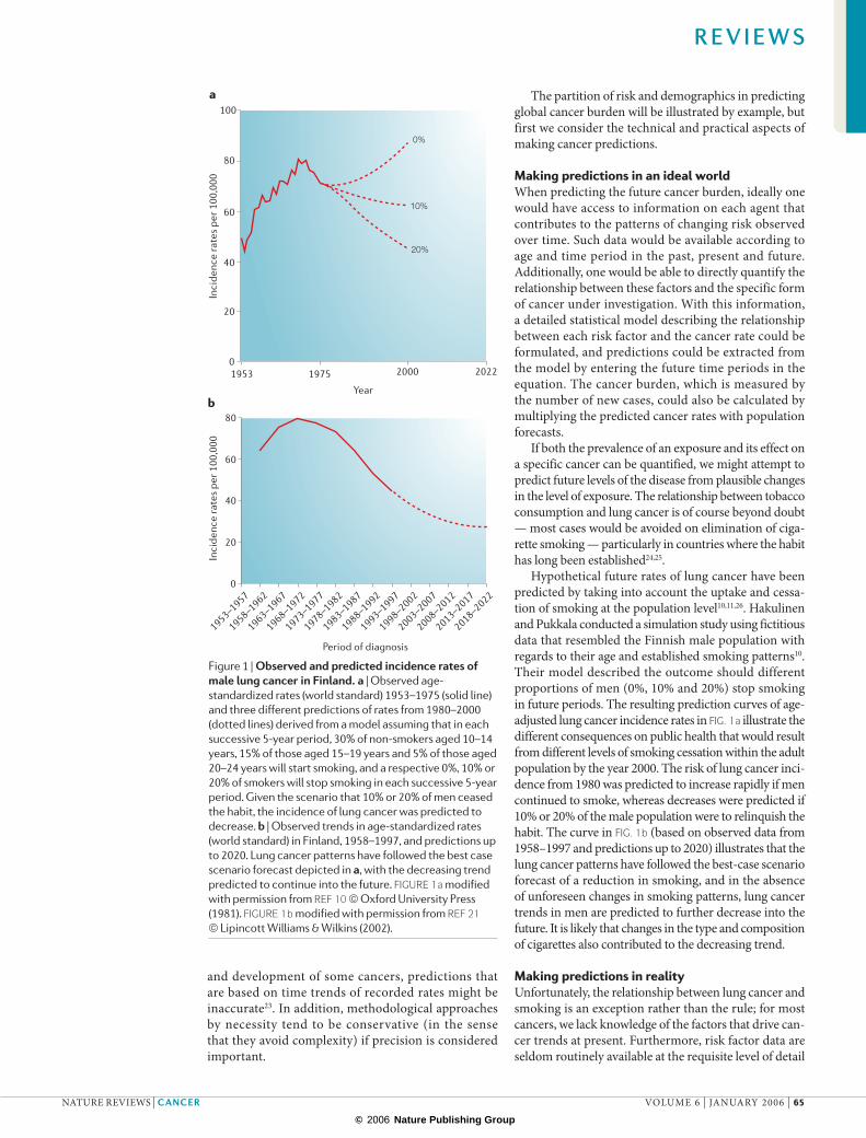
Hypothetical future rates of lung cancer have been predicted by taking into account the uptake and cessa-tion of smoking at the population level10,11,26. Hakulinen and Pukkala conducted a simulation study using fictitious data that resembled the Finnish male population with regards to their age and established smoking patterns10. Their model described the outcome should different proportions of men (0%, 10% and 20%) stop smoking in future periods. The resulting prediction curves of age-adjusted lung cancer incidence rates in FIG. 1a illustrate the different consequences on public health that would result from different levels of smoking cessation within the adult population by the year 2000. The risk of lung cancer inci-dence from 1980 was predicted to increase rapidly if men continued to smoke, whereas decreases were predicted if 10% or 20% of the male population were to relinquish the habit. The curve in FIG. 1b (based on observed data from 1958–1997 and predictions up to 2020) illustrates that the lung cancer patterns have followed the best-case scenario forecast of a reduction in smoking, and in the absence of unforeseen changes in smoking patterns, lung cancer trends in men are predicted to further decrease into the future. It is likely that changes in the type and composition of cigarettes also contributed to the decreasing trend.

Making predictions in realityUnfortunately, the relationship between lung cancer and smoking is an exception rather than the rule; for most cancers, we lack knowledge of the factors that drive can-cer trends at present. Furthermore, risk factor data are seldom routinely available at the requisite level of detail

Figure 1 | Observed and predicted incidence rates of male lung cancer in Finland. a | Observed age-standardized rates (world standard) 1953–1975 (solid line) and three different predictions of rates from 1980–2000 (dotted lines) derived from a model assuming that in each successive 5-year period, 30% of non-smokers aged 10–14 years, 15% of those aged 15–19 years and 5% of those aged 20–24 years will start smoking, and a respective 0%, 10% or 20% of smokers will stop smoking in each successive 5-year period. Given the scenario that 10% or 20% of men ceased the habit, the incidence of lung cancer was predicted to decrease. b | Observed trends in age-standardized rates (world standard) in Finland, 1958–1997, and predictions up to 2020. Lung cancer patterns have followed the best case scenario forecast depicted in a, with the decreasing trend predicted to continue into the future. FIGURE 1a modified with permission from REF 10 © Oxford University Press (1981). FIGURE 1b modified with permission from REF 21 © Lipincott Williams & Wilkins (2002).

R E V I E W S



70

60

50

40

302000

Age

(yea

rs)

1960 1970 1980 1990

Calendar time

1930

1930

1930

1930

1930

1930

1930

1930

Age–period–cohort analyses Tabulations and analyses of rates by age, period and birth cohort to determine their effects. Often involves use of the age–period–cohort model, which is used when it is reasonable to assume that both period and cohort influence disease risk.

Poisson distributionA distribution used to describe counts of rare events. The distribution is used in a Poisson regression to model incidence and mortality rates in populations over time.

— by sex, age group and calendar time — and in any case, few associations between a single risk factor and the onset of cancer are strong enough to be modelled directly. Therefore, in most instances predictions are based on extrapolations of past trends in three time-related variables — age, period and cohort — the char-acteristics of which are described below. The statistical model that is most commonly used in prediction is the age–period–cohort model27, in which the period and birth cohort effects are proxies for events such as risk factors, which we often cannot measure directly28,29.

Quantitatively, the most important time-related variable that influences the risk of cancer is age. Cancer incidence rates usually increase with age, and for the epithelial cancers, the risk increases at approximately the fifth to sixth power of age30, representing up to a 1000-fold difference in cancer rates between young (aged 20) and old people (aged 80)31. Ageing charac-terizes the cumulative exposure of the body to carcino-gens over time, and the accumulation of the series of mutations that are necessary for the unregulated cell proliferation that leads to cancer32.

Period effects are indicated by an immediate, or delayed but pre-determined, change in rates in each age group, and therefore relate to events that quickly change incidence or mortality with the same order of magnitude regardless of the age group under study. They often transpire from changes in classification criteria or the availability of new

diagnostic tests, although the introduction of a powerful carcinogen or a screening intervention (that affects all studied age groups) might also show up a period effect. With respect to cancer mortality, advances in treatment (across age groups) would also generally be evident as a period effect on mortality.

Cohort effects cause changes in incidence rates from one generation to another that are consistent across age groups. Routine data on cancer occurrence (from cancer registries) and cancer deaths (from mortality registers such as the World Health Organization (WHO) mortality databank) are available in 5-year age groups and 5-year time periods. Synthetic birth cohorts might therefore be obtained by subtracting age (the midpoint of the 5-year age band) from the central year of the 5-year period of diagnosis (BOX 1). Cohort effects might relate (or seem to relate) to date of birth itself as they involve factors that are shared by a particular generation as they age together. Many lifestyle factors, such as tobacco smoking, sexual behaviour and reproductive behaviour, tend to be generation-specific. Given that many forms of cancer have a long induction phase, birth-cohort analysis plays an important part in confirming (or occasionally refut-ing) evidence of the role of putative aetiological factors from other types of epidemiological study.

Difficulties in projecting age, period and cohort into the future. A selection of methods that are used for the prediction of cancer rates are given in BOX 2. Applying the age–period–cohort model to making predictions usually involves estimating the underlying age-, period- and cohort-specific trends and projecting them into the future using a Poisson regression model. The three components are mutually dependent because, for a given date of birth and age, the time period is locked. One consequence of this interrelationship is that it is possible to estimate the average increase over time, but not to assess whether an average increase over time is caused by period-specific factors (such as changes in new diagnostic tests), or by cohort-specific factors (for example, steady changes in smoking habits in consecu-tive cohorts). This average underlying trend, common for period and cohort, has been termed the ‘drift’33. It is only possible to identify time periods and birth cohorts that deviate from this average slope.

It is possible that projection of this drift into the future would not produce more accurate predictions of events than assuming that future rates remain constant at the present level. However, an empirical study of cancer incidence in the Nordic countries showed that projecting current trends, rather than simply using a constant rate, resulted in predictions that were closer to rates that were observed 10 years later34. Allowing for a gradual damp-ening of the impact of current trends in future periods improved the predictions, whereas following the most recent trends (instead of the average trend over the whole observation period) resulted in further improvements. Tiwari and co-workers had a similar experience when analysing US mortality data, in which they found that a new method aimed at pursuing recent changes in the rates improved predictions 3 years ahead35.

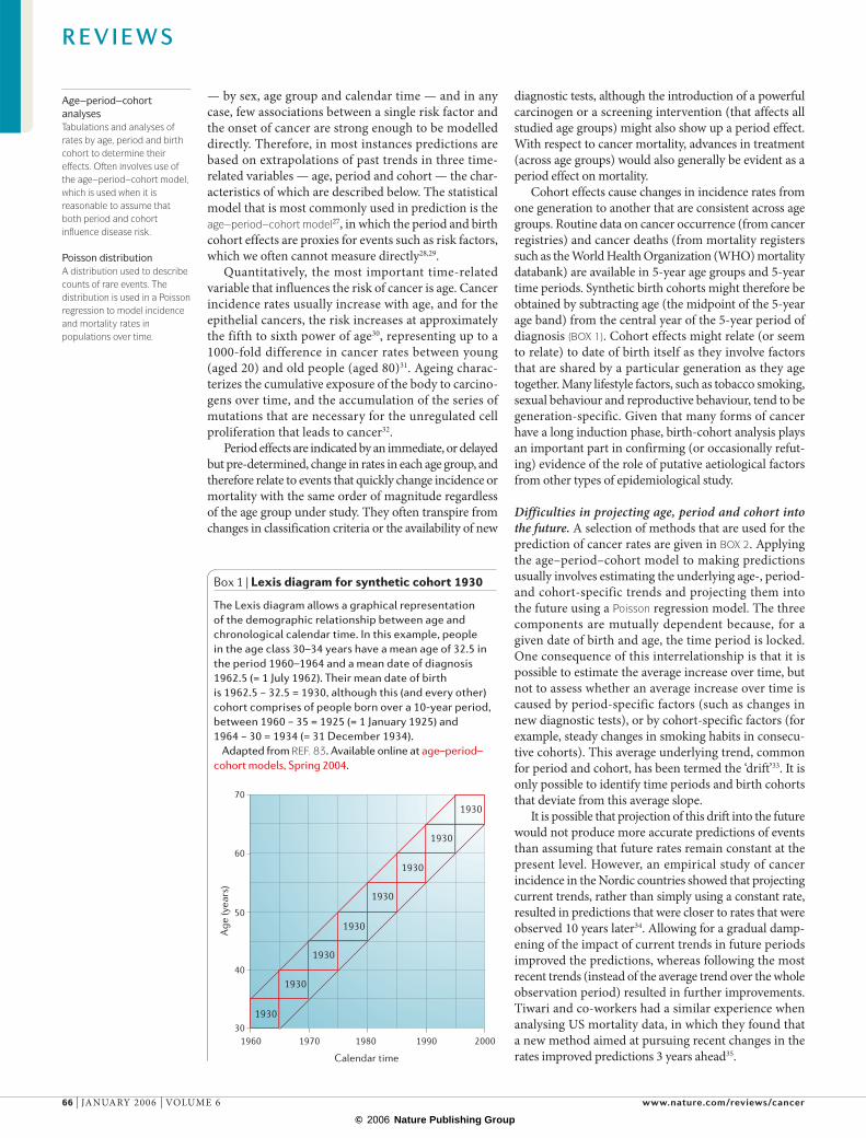
Box 1 | Lexis diagram for synthetic cohort 1930

The Lexis diagram allows a graphical representation of the demographic relationship between age and chronological calendar time. In this example, people in the age class 30–34 years have a mean age of 32.5 in the period 1960–1964 and a mean date of diagnosis 1962.5 (= 1 July 1962). Their mean date of birth is 1962.5 − 32.5 = 1930, although this (and every other) cohort comprises of people born over a 10-year period, between 1960 − 35 = 1925 (= 1 January 1925) and 1964 − 30 = 1934 (= 31 December 1934).

Adapted from REF. 83. Available online at age–period–cohort models, Spring 2004.

R E V I E W S



Prediction intervalsRange of possible future observations that take into account the random variation inherent in the past trends as well as the future prediction.

Complexities in using routine data sources. The inter-pretation of trends in cancer incidence and mortality data requires a profound understanding of the properties and potential caveats that are associated with their use36. Incidence data are obtained from population-based can-cer registries that collect, store and analyse information on all new cases of cancer in well-defined populations. At present, registries cover about one-fifth of the world population, with more than two-thirds coverage in developed areas but less than 10% of developing areas. Cancer registration, however, continues to expand; the most recent volume of Cancer Incidence in Five Continents contains high-quality, comparable incidence data (mainly for the registration period 1993–1997) from 186 registries in 57 countries37.

Mortality data come from regional or national offices that are responsible for the collation of infor-mation on the causes of death of the inhabitants of that region or nation, and are compiled at the international level in the WHO mortality databank. The relative strengths and weaknesses of cancer incidence and mortality data in studying temporal patterns are well known36,38–41. For instance, changing completeness of registration (the extent to which all cases in the target population are included in the registry), improving diagnostic methods, and inaccuracies in population estimates might unduly bias incidence trends. However, in the absence of such artefacts, changes in incidence convey how the average risk of developing cancer in

the population changes over time, signalling changes in the prevalence and distribution of environmental exposures, which are time-lagged by an approximation of the latency period.

Mortality statistics are produced according to the underlying cause of death, although this might not equate with the presence of a particular tumour and might be subject to change with time. Aside from arte-facts that are related to registration practices, the factors that affect incidence equally apply to mortality data, although sometimes with a different level of intensity38. The advantage of mortality data is their comprehensive availability at the national level over long periods of time. Mortality trends measure changes in the average risk in the population of dying from the disease and describe, in addition to the underlying incidence, case fatality — the outcome or impact of cancer. Mortality data might therefore be a rather poor proxy of incidence rates if prognosis has improved with time and case fatal-ity does not remain constant. One of the crucial merits of mortality rates versus incidence, however, remains the evaluation of certain screening programmes as well as the role of therapy and cancer care.

Given that cancer represents a diverse group of diseases rather than a single disease, the particular problems with the reliability of incidence and mortality must be consid-ered separately for each form of cancer, its site of origin and its histology. Incidence data are expected to be, in general, of better diagnostic quality than mortality data, and, in the planning of services, are expected to provide a more pertinent estimate of the future needs of cancer services.

Examples of predictions in practiceMuch of the contemporary work on making predictions of cancer, from both a theoretical and practical perspec-tive, stems from scientists who work at the Finnish Cancer Registry. Their first report, which involved predictions of the 12 most common forms of cancers in Finland for 1980, was published in 1974, based on the linear extrapo-lation of trends from 1957–1968 (REFS 42,43). Prediction techniques have allowed the estimation of prediction intervals based on simple linear Poisson models44,45. An empirical comparison of 15 different age–period–cohort prediction methods34 provided some practical advice on making predictions (described in BOX 3).

Some of these technical developments have been incorporated into the study of cancer trends and pre-dictions in the five Nordic countries, most recently for 2010 and 2020, based on classical age–period–cohort models21,46. Coory and Armstrong have used Bayesian age–period–cohort models to project incidence for-ward to the time period 2001–2006 by health services area in New South Wales, Australia47. A compre-hensive survey of various prediction techniques and their application to the future cancer burden in New Zealand up to 2010 (to aid the formulation of a cancer control plan) is available in Cancer in New Zealand: Trends and Projections48.

The innovative Cancer Scenarios project in Scotland went further by asking specialists to specu-late on whether preventative and treatment-based

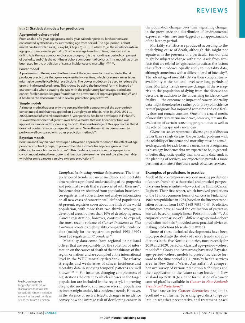
Box 2 | Statistical models for predictions

Age–period–cohort modelFrom a table of 5-year age groups and 5-year calendar periods, birth cohorts are constructed synthetically by subtracting age from period. The age–period–cohort model can be written as: Rap = exp(Aa + D∙p + Pp + Cc), in which Rap is the incidence rate in age group a in calendar period p; D is the average trend with time, denoted as the drift33; Aa is the age component for age group a; Pp is the non-linear period component of period p; and Cc is the non-linear cohort component of cohort c. This model has often been used for the prediction of cancer incidence and mortality18,49,78–80.

Power modelA problem with the exponential function of the age–period–cohort model is that it produces predictions that grow exponentially over time, which for some cancer types might give unrealistically high predictions. The power model can be used to reduce the growth in the predicted rates. This is done by using the functional form x5 instead of exponential x when equating the rate with the explanatory factors age, period and cohort. Møller and colleagues found that the power model improved predictions34, and it has been the chosen method in several prediction projects21,46,68.

Simple modelsA simpler model that uses only the age and the drift component of the age–period–cohort model and that was applied on 11 single years (that is, rates in 1990, 1991 … 2000), instead of several consecutive 5-year periods, has been developed in Finland71. To avoid the exponential growth over time, a model that was linear over time was applied for cancers with increasing trends45. The disadvantage of this approach is that it does not contain any cohort-specific patterns. Nevertheless, it has been shown to perform well compared with other prediction methods34.

Bayesian modelsBerzuini and Clayton have developed a Bayesian approach to smooth the effects of age, period and cohort groups, to prevent the rate estimate for adjacent groups from differing too much from each other81. This model originates from the age–period–cohort model, using the exponential function between the rate and the effect variables, which for some cancers can give extreme predictions82.

R E V I E W S



Risk factorsor screening

practice

Future trend directionbased on current

observed trend

No reliable time trend of ratesbut future trend direction based

on external source

Population forecasts and recent cancer rate,but no reliable time trend of rates

Long term data on colon cancer incidence in the Nordic countries

Assumption of increasing riskapplied to breast and prostatecancer worldwide

Recent rates for all sites worldwide combined with population forecasts

Incr

easi

ng a

vaila

bilit

y of

dat

a

Incr

easi

ng m

odel

ling

poss

ibili

ty

Examples

Mammographic screeningand breast cancer in the Nordic countries

interventions could modify the incidence and mor-tality trends projected up to and including the period 2010–2014 (REF. 20). Predictions of cancer are now commonplace in peer-reviewed medical and epide-miological articles. Predicting the epidemics of lung cancer in relation to smoking10,11,26,49–53, and mesothe-lioma following exposure to asbestos54–58 have been particularly intensively researched.

Four examples of cancer predictions are provided below that, given the increasing availability of relevant data, might also involve an increasing level of analytical complexity. FIGURE 2 gives an illustration of this con-cept. We begin with global projections of cancer based on combining current cancer rates with population forecasts and then add speculations of the future linear trend. We then turn our attention to the provision of national estimates involving projections of age, period

and birth cohort components, concluding with an example that incorporates additional information on breast cancer screening.

Estimating overall cancer incidence worldwide. Making projections of cancer occurrence at the global level is complicated; recent trends in different age groups (or birth cohorts) are often heterogeneous in magnitude and direction, as are the composite past trends in dif-ferent regions of the world. Furthermore, we lack detailed information on changes in the age-specific incidence in many areas of the world. A comprehensive set of projections of future cancer burden at the world level must therefore involve an assessment of projected demographic changes, assuming either that current rates remain the same into the future or that they are modified by a specific future change in incidence.

The effect of structural changes in the population substantially alters the expected number of future cases. On a global scale, the slow decrease in fertility along-side an increase in life expectancy that is projected over the next 50 years will have important consequences on the burden of disability and chronic diseases59, the demands and delivery of health services and the future allocation of resources for them.

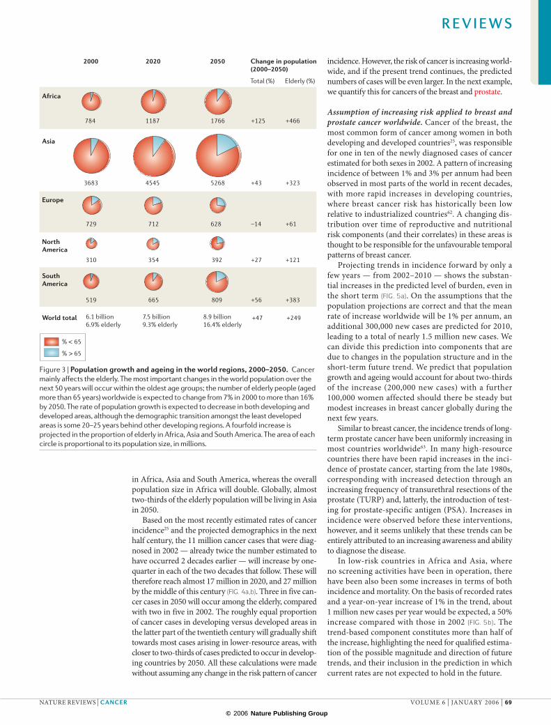
Cancer mainly affects the elderly. The most recent estimates of worldwide cancer burden indicate that about 45% of cancers occurred in people aged 65 years or over in 2002 (REF. 60). The world’s population has grown from 2.8 billion in 1955 to more than 6 billion in 2000 (REF. 61). Barring a catastrophe, the population will increase to 7.5 billion by 2020 and to 8.9 billion by 2050 (FIG. 3), a projected increase of nearly 80 million people a year. It is forecast that population size will peak in developed countries around 2020 and then decrease — by 2050, the overall population in developed coun-tries should be some 2% less than the 2000 estimate (FIG. 3). The population size in Europe, for instance, will, if anything, decrease in the next 50 years. This contrasts strongly with the situation in less developed countries. A fourfold increase is projected in the proportion of elderly

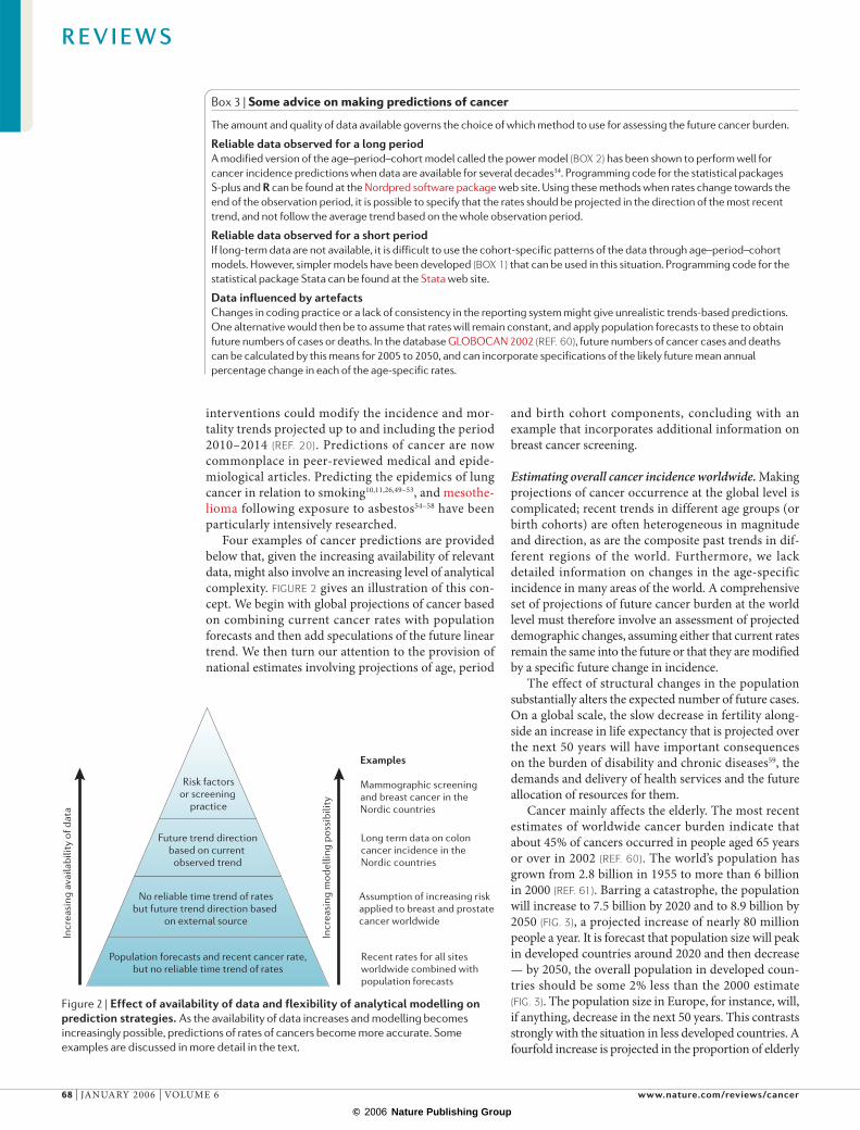
Box 3 | Some advice on making predictions of cancer

The amount and quality of data available governs the choice of which method to use for assessing the future cancer burden.

Reliable data observed for a long periodA modified version of the age–period–cohort model called the power model (BOX 2) has been shown to perform well for cancer incidence predictions when data are available for several decades34. Programming code for the statistical packages S-plus and R can be found at the Nordpred software package web site. Using these methods when rates change towards the end of the observation period, it is possible to specify that the rates should be projected in the direction of the most recent trend, and not follow the average trend based on the whole observation period.

Reliable data observed for a short periodIf long-term data are not available, it is difficult to use the cohort-specific patterns of the data through age–period–cohort models. However, simpler models have been developed (BOX 1) that can be used in this situation. Programming code for the statistical package Stata can be found at the Stata web site.

Data influenced by artefactsChanges in coding practice or a lack of consistency in the reporting system might give unrealistic trends-based predictions. One alternative would then be to assume that rates will remain constant, and apply population forecasts to these to obtain future numbers of cases or deaths. In the database GLOBOCAN 2002 (REF. 60), future numbers of cancer cases and deaths can be calculated by this means for 2005 to 2050, and can incorporate specifications of the likely future mean annual percentage change in each of the age-specific rates.

Figure 2 | Effect of availability of data and flexibility of analytical modelling on prediction strategies. As the availability of data increases and modelling becomes increasingly possible, predictions of rates of cancers become more accurate. Some examples are discussed in more detail in the text.

R E V I E W S



Africa

2000 2020 2050 Change in population(2000–2050)

Total (%) Elderly (%)

784 1187 1766 +125 +466

Asia

3683 4545 5268 +43 +323

Europe

729 712 628 –14 +61

North America

310 354 392 +27 +121

South America

World total

519 665 809

6.1 billion6.9% elderly



+56 +383

+47 +249

% < 65

% > 65

in Africa, Asia and South America, whereas the overall population size in Africa will double. Globally, almost two-thirds of the elderly population will be living in Asia in 2050.

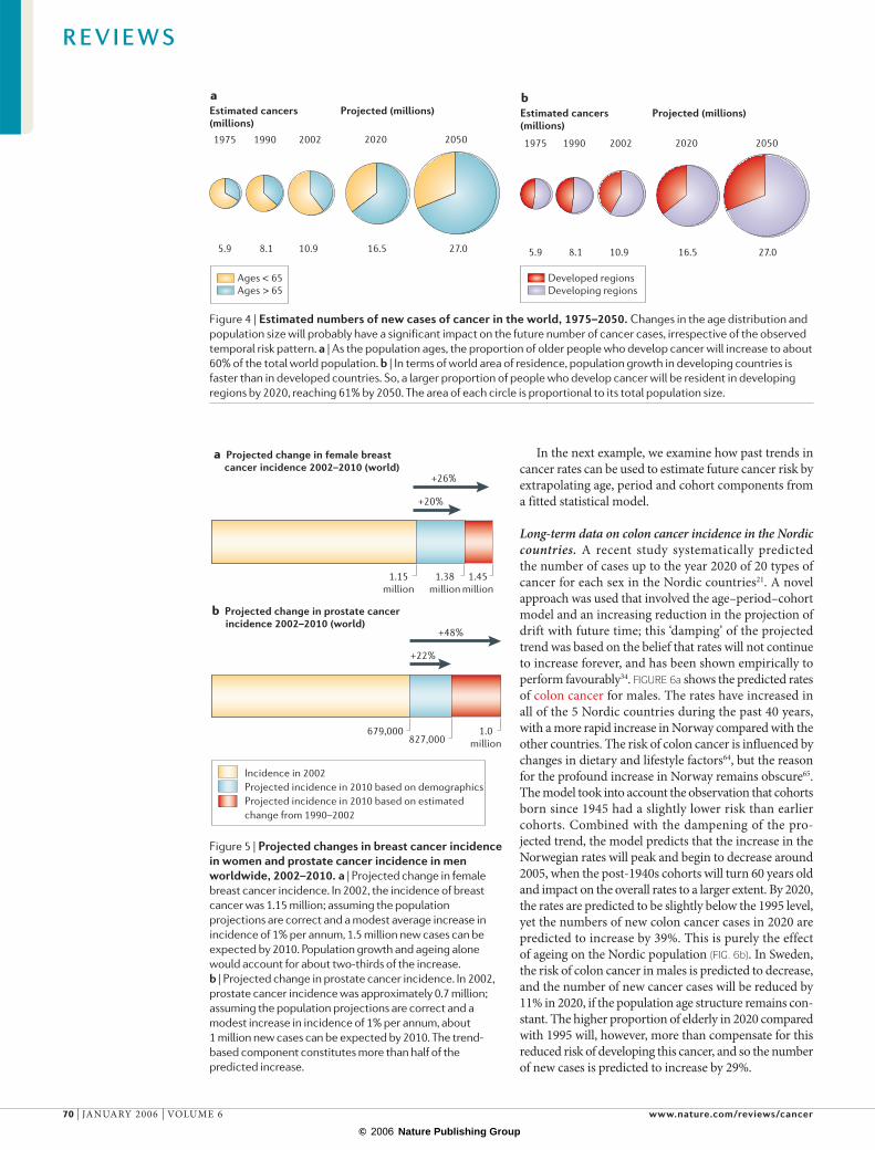
Based on the most recently estimated rates of cancer incidence25 and the projected demographics in the next half century, the 11 million cancer cases that were diag-nosed in 2002 — already twice the number estimated to have occurred 2 decades earlier — will increase by one-quarter in each of the two decades that follow. These will therefore reach almost 17 million in 2020, and 27 million by the middle of this century (FIG. 4a,b). Three in five can-cer cases in 2050 will occur among the elderly, compared with two in five in 2002. The roughly equal proportion of cancer cases in developing versus developed areas in the latter part of the twentieth century will gradually shift towards most cases arising in lower-resource areas, with closer to two-thirds of cases predicted to occur in develop-ing countries by 2050. All these calculations were made without assuming any change in the risk pattern of cancer

incidence. However, the risk of cancer is increasing world-wide, and if the present trend continues, the predicted numbers of cases will be even larger. In the next example, we quantify this for cancers of the breast and prostate.

Assumption of increasing risk applied to breast and prostate cancer worldwide. Cancer of the breast, the most common form of cancer among women in both developing and developed countries25, was responsible for one in ten of the newly diagnosed cases of cancer estimated for both sexes in 2002. A pattern of increasing incidence of between 1% and 3% per annum had been observed in most parts of the world in recent decades, with more rapid increases in developing countries, where breast cancer risk has historically been low relative to industrialized countries62. A changing dis-tribution over time of reproductive and nutritional risk components (and their correlates) in these areas is thought to be responsible for the unfavourable temporal patterns of breast cancer.

Projecting trends in incidence forward by only a few years — from 2002–2010 — shows the substan-tial increases in the predicted level of burden, even in the short term (FIG. 5a). On the assumptions that the population projections are correct and that the mean rate of increase worldwide will be 1% per annum, an additional 300,000 new cases are predicted for 2010, leading to a total of nearly 1.5 million new cases. We can divide this prediction into components that are due to changes in the population structure and in the short-term future trend. We predict that population growth and ageing would account for about two-thirds of the increase (200,000 new cases) with a further 100,000 women affected should there be steady but modest increases in breast cancer globally during the next few years.

Similar to breast cancer, the incidence trends of long-term prostate cancer have been uniformly increasing in most countries worldwide63. In many high-resource countries there have been rapid increases in the inci-dence of prostate cancer, starting from the late 1980s, corresponding with increased detection through an increasing frequency of transurethral resections of the prostate (TURP) and, latterly, the introduction of test-ing for prostate-specific antigen (PSA). Increases in incidence were observed before these interventions, however, and it seems unlikely that these trends can be entirely attributed to an increasing awareness and ability to diagnose the disease.

In low-risk countries in Africa and Asia, where no screening activities have been in operation, there have been also been some increases in terms of both incidence and mortality. On the basis of recorded rates and a year-on-year increase of 1% in the trend, about 1 million new cases per year would be expected, a 50% increase compared with those in 2002 (FIG. 5b). The trend-based component constitutes more than half of the increase, highlighting the need for qualified estima-tion of the possible magnitude and direction of future trends, and their inclusion in the prediction in which current rates are not expected to hold in the future.

Figure 3 | Population growth and ageing in the world regions, 2000–2050. Cancer mainly affects the elderly. The most important changes in the world population over the next 50 years will occur within the oldest age groups; the number of elderly people (aged more than 65 years) worldwide is expected to change from 7% in 2000 to more than 16% by 2050. The rate of population growth is expected to decrease in both developing and developed areas, although the demographic transition amongst the least developed areas is some 20–25 years behind other developing regions. A fourfold increase is projected in the proportion of elderly in Africa, Asia and South America. The area of each circle is proportional to its population size, in millions.

R E V I E W S



1975 1990 2002

5.9 8.1 10.9

2020 2050

16.5 27.0

Estimated cancers (millions)

1975 1990 2002

5.9 8.1 10.9

Projected (millions)

2020 2050

16.5 27.0

bEstimated cancers (millions)

Projected (millions)a

Ages < 65Ages > 65

Developed regionsDeveloping regions

1.15million

1.38million

1.45million

679,000827,000

1.0million

a Projected change in female breast cancer incidence 2002–2010 (world)

+26%

+20%

b Projected change in prostate cancer incidence 2002–2010 (world)

+48%

+22%

Incidence in 2002Projected incidence in 2010 based on demographicsProjected incidence in 2010 based on estimated change from 1990–2002

In the next example, we examine how past trends in cancer rates can be used to estimate future cancer risk by extrapolating age, period and cohort components from a fitted statistical model.

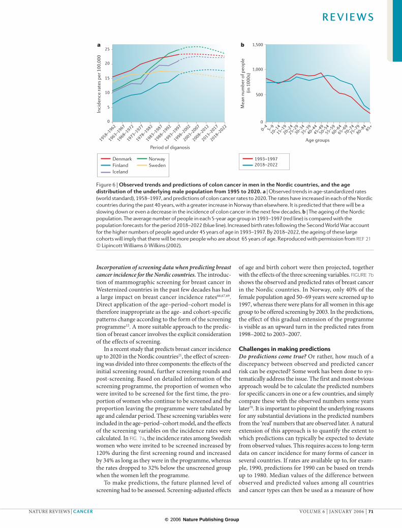
Long-term data on colon cancer incidence in the Nordic countries. A recent study systematically predicted the number of cases up to the year 2020 of 20 types of cancer for each sex in the Nordic countries21. A novel approach was used that involved the age–period–cohort model and an increasing reduction in the projection of drift with future time; this ‘damping’ of the projected trend was based on the belief that rates will not continue to increase forever, and has been shown empirically to perform favourably34. FIGURE 6a shows the predicted rates of colon cancer for males. The rates have increased in all of the 5 Nordic countries during the past 40 years, with a more rapid increase in Norway compared with the other countries. The risk of colon cancer is influenced by changes in dietary and lifestyle factors64, but the reason for the profound increase in Norway remains obscure65. The model took into account the observation that cohorts born since 1945 had a slightly lower risk than earlier cohorts. Combined with the dampening of the pro-jected trend, the model predicts that the increase in the Norwegian rates will peak and begin to decrease around 2005, when the post-1940s cohorts will turn 60 years old and impact on the overall rates to a larger extent. By 2020, the rates are predicted to be slightly below the 1995 level, yet the numbers of new colon cancer cases in 2020 are predicted to increase by 39%. This is purely the effect of ageing on the Nordic population (FIG. 6b). In Sweden, the risk of colon cancer in males is predicted to decrease, and the number of new cancer cases will be reduced by 11% in 2020, if the population age structure remains con-stant. The higher proportion of elderly in 2020 compared with 1995 will, however, more than compensate for this reduced risk of developing this cancer, and so the number of new cases is predicted to increase by 29%.

Figure 4 | Estimated numbers of new cases of cancer in the world, 1975–2050. Changes in the age distribution and population size will probably have a significant impact on the future number of cancer cases, irrespective of the observed temporal risk pattern. a | As the population ages, the proportion of older people who develop cancer will increase to about 60% of the total world population. b | In terms of world area of residence, population growth in developing countries is faster than in developed countries. So, a larger proportion of people who develop cancer will be resident in developing regions by 2020, reaching 61% by 2050. The area of each circle is proportional to its total population size.

Figure 5 | Projected changes in breast cancer incidence in women and prostate cancer incidence in men worldwide, 2002–2010. a | Projected change in female breast cancer incidence. In 2002, the incidence of breast cancer was 1.15 million; assuming the population projections are correct and a modest average increase in incidence of 1% per annum, 1.5 million new cases can be expected by 2010. Population growth and ageing alone would account for about two-thirds of the increase. b | Projected change in prostate cancer incidence. In 2002, prostate cancer incidence was approximately 0.7 million; assuming the population projections are correct and a modest increase in incidence of 1% per annum, about 1 million new cases can be expected by 2010. The trend-based component constitutes more than half of the predicted increase.

R E V I E W S



1998–2002

2003–2007

2008–2012

2013–2017

2018–2022

1973–1977

1978–1982

1983–1987

1988–1992

1993–1997

1958–1962

1963–1967

1968–19720–4

5–910–14

15–1920–24

25–2930–34

35–3940–44

45–4950–54

55–5960–64

65–6970–74

75–7980–84

85+

25

20

15

10

5

0

1,500

1,000

500

0

Period of diganosis

a b

Mea

n nu

mbe

r of p

eopl

e (in

100

0s)

Inci

denc

e ra

tes

per 1

00,0

00

Age groups

DenmarkFinlandIceland

NorwaySweden

1993–19972018–2022

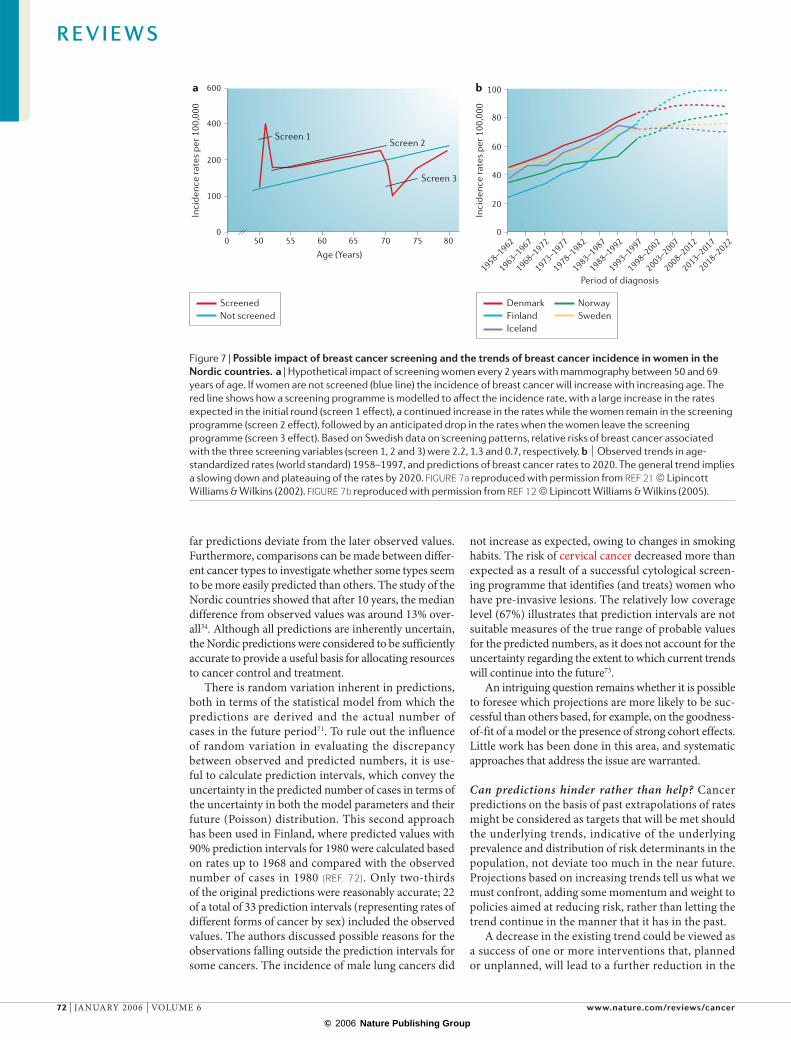
Incorporation of screening data when predicting breast cancer incidence for the Nordic countries. The introduc-tion of mammographic screening for breast cancer in Westernized countries in the past few decades has had a large impact on breast cancer incidence rates66,67,69. Direct application of the age–period–cohort model is therefore inappropriate as the age- and cohort-specific patterns change according to the form of the screening programme12. A more suitable approach to the predic-tion of breast cancer involves the explicit consideration of the effects of screening.

In a recent study that predicts breast cancer incidence up to 2020 in the Nordic countries21, the effect of screen-ing was divided into three components: the effects of the initial screening round, further screening rounds and post-screening. Based on detailed information of the screening programme, the proportion of women who were invited to be screened for the first time, the pro-portion of women who continue to be screened and the proportion leaving the programme were tabulated by age and calendar period. These screening variables were included in the age–period–cohort model, and the effects of the screening variables on the incidence rates were calculated. In FIG. 7a, the incidence rates among Swedish women who were invited to be screened increased by 120% during the first screening round and increased by 34% as long as they were in the programme, whereas the rates dropped to 32% below the unscreened group when the women left the programme.

To make predictions, the future planned level of screening had to be assessed. Screening-adjusted effects

of age and birth cohort were then projected, together with the effects of the three screening variables. FIGURE 7b shows the observed and predicted rates of breast cancer in the Nordic countries. In Norway, only 40% of the female population aged 50–69 years were screened up to 1997, whereas there were plans for all women in this age group to be offered screening by 2003. In the predictions, the effect of this gradual extension of the programme is visible as an upward turn in the predicted rates from 1998–2002 to 2003–2007.

Challenges in making predictionsDo predictions come true? Or rather, how much of a discrepancy between observed and predicted cancer risk can be expected? Some work has been done to sys-tematically address the issue. The first and most obvious approach would be to calculate the predicted numbers for specific cancers in one or a few countries, and simply compare these with the observed numbers some years later70. It is important to pinpoint the underlying reasons for any substantial deviations in the predicted numbers from the ‘real’ numbers that are observed later. A natural extension of this approach is to quantify the extent to which predictions can typically be expected to deviate from observed values. This requires access to long-term data on cancer incidence for many forms of cancer in several countries. If rates are available up to, for exam-ple, 1990, predictions for 1990 can be based on trends up to 1980. Median values of the difference between observed and predicted values among all countries and cancer types can then be used as a measure of how

Figure 6 | Observed trends and predictions of colon cancer in men in the Nordic countries, and the age distribution of the underlying male population from 1995 to 2020. a | Observed trends in age-standardized rates (world standard), 1958–1997, and predictions of colon cancer rates to 2020. The rates have increased in each of the Nordic countries during the past 40 years, with a greater increase in Norway than elsewhere. It is predicted that there will be a slowing down or even a decrease in the incidence of colon cancer in the next few decades. b | The ageing of the Nordic population. The average number of people in each 5-year age group in 1993–1997 (red line) is compared with the population forecasts for the period 2018–2022 (blue line). Increased birth rates following the Second World War account for the higher numbers of people aged under 45 years of age in 1993–1997. By 2018–2022, the ageing of these large cohorts will imply that there will be more people who are about 65 years of age. Reproduced with permission from REF 21 © Lipincott Williams & Wilkins (2002).

R E V I E W S



1998–2002

2003–2007

2008–2012

2013–2017

2018–2022

1973–1977

1978–1982

1983–1987

1988–1992

1993–1997

1958–1962

1963–1967

1968–1972

100

80

60

40

20

0

ba

Period of diagnosis

DenmarkFinlandIceland

NorwaySweden

ScreenedNot screened

400

200

600

100

00 50 55 60 65 70 75 80

Age (Years)

Inci

denc

e ra

tes

per 1

00,0

00

Inci

denc

e ra

tes

per 1

00,0

00

Screen 1Screen 2

Screen 3

far predictions deviate from the later observed values. Furthermore, comparisons can be made between differ-ent cancer types to investigate whether some types seem to be more easily predicted than others. The study of the Nordic countries showed that after 10 years, the median difference from observed values was around 13% over-all34. Although all predictions are inherently uncertain, the Nordic predictions were considered to be sufficiently accurate to provide a useful basis for allocating resources to cancer control and treatment.

There is random variation inherent in predictions, both in terms of the statistical model from which the predictions are derived and the actual number of cases in the future period71. To rule out the influence of random variation in evaluating the discrepancy between observed and predicted numbers, it is use-ful to calculate prediction intervals, which convey the uncertainty in the predicted number of cases in terms of the uncertainty in both the model parameters and their future (Poisson) distribution. This second approach has been used in Finland, where predicted values with 90% prediction intervals for 1980 were calculated based on rates up to 1968 and compared with the observed number of cases in 1980 (REF. 72). Only two-thirds of the original predictions were reasonably accurate; 22 of a total of 33 prediction intervals (representing rates of different forms of cancer by sex) included the observed values. The authors discussed possible reasons for the observations falling outside the prediction intervals for some cancers. The incidence of male lung cancers did

not increase as expected, owing to changes in smoking habits. The risk of cervical cancer decreased more than expected as a result of a successful cytological screen-ing programme that identifies (and treats) women who have pre-invasive lesions. The relatively low coverage level (67%) illustrates that prediction intervals are not suitable measures of the true range of probable values for the predicted numbers, as it does not account for the uncertainty regarding the extent to which current trends will continue into the future73.

An intriguing question remains whether it is possible to foresee which projections are more likely to be suc-cessful than others based, for example, on the goodness-of-fit of a model or the presence of strong cohort effects. Little work has been done in this area, and systematic approaches that address the issue are warranted.

Can predictions hinder rather than help? Cancer predictions on the basis of past extrapolations of rates might be considered as targets that will be met should the underlying trends, indicative of the underlying prevalence and distribution of risk determinants in the population, not deviate too much in the near future. Projections based on increasing trends tell us what we must confront, adding some momentum and weight to policies aimed at reducing risk, rather than letting the trend continue in the manner that it has in the past.

A decrease in the existing trend could be viewed as a success of one or more interventions that, planned or unplanned, will lead to a further reduction in the

Figure 7 | Possible impact of breast cancer screening and the trends of breast cancer incidence in women in the Nordic countries. a | Hypothetical impact of screening women every 2 years with mammography between 50 and 69 years of age. If women are not screened (blue line) the incidence of breast cancer will increase with increasing age. The red line shows how a screening programme is modelled to affect the incidence rate, with a large increase in the rates expected in the initial round (screen 1 effect), a continued increase in the rates while the women remain in the screening programme (screen 2 effect), followed by an anticipated drop in the rates when the women leave the screening programme (screen 3 effect). Based on Swedish data on screening patterns, relative risks of breast cancer associated with the three screening variables (screen 1, 2 and 3) were 2.2, 1.3 and 0.7, respectively. b | Observed trends in age-standardized rates (world standard) 1958–1997, and predictions of breast cancer rates to 2020. The general trend implies a slowing down and plateauing of the rates by 2020. FIGURE 7a reproduced with permission from REF 21 © Lipincott Williams & Wilkins (2002). FIGURE 7b reproduced with permission from REF 12 © Lipincott Williams & Wilkins (2005).

R E V I E W S



rate in the future. Well-established examples include the decrease in incidence of stomach cancer (in most countries worldwide) and cervical cancer (in countries where Pap screening was introduced). One potential danger that is inherent in predictions of decreasing incidence is that they might lead to some degree of complacency in the users of such information. By creating a situation in which the need for vigilant monitoring of the trends and consequent preventa-tive actions could be considered less acute, there is a risk that sudden unexpected changes in the disease trends might go unnoticed as planners transfer their attention elsewhere.

The point is illustrated by predictions of cervi-cal cancer incidence in Finland for 2000 and 2010 obtained from the trends from 1958–1987 (REF. 46). Cervical cancer incidence and mortality rates decreased rapidly in Finland between the mid-1960s and mid-1980s, largely a result of the successful imple-mentation (in 1963) of a nationally organized screen-ing programme74. The predicted incidence rates of 2.2 per 100,000 for 1998–2002 were almost half those observed in 2000, a result of unanticipated increases in cervical cancer incidence during the 1990s. In this example, explanations for the sudden rise in incidence were sought. The rises were seen in younger women below the age of 55 years (REF. 75) and attributed to changing sexual lifestyles and increased trans-mission of papillomaviruses in younger generations of women76, to shortfalls in screening attendance76, and more recently to the quality and criteria of cytological laboratory procedures during this time77. As predic-tions could contribute to complacency, predictions should be continuously monitored, deviations in the prediction from that expected investigated, and find-ings acted on.

A key aspect of prediction of future numbers of cases and deaths relates to the impact of population growth and ageing. Changes in the size and (particularly) ageing of the population often constitute a larger component of predicted increases in burden than corresponding changes in risk. Indeed, predicted increases in the abso-lute numbers might arise from demographic changes even when existing trends are stable or decreasing. It is therefore important that the potential for misinterpreta-tion is minimized by focusing on the impact of risk and the reduction of risk through prevention.

The impact of ageing on cancer is sometimes neglected in interpreting predictions. It is inevitable that much of the future burden will be among the elderly, and for which a proportion of the cancers diagnosed will remain incurable. Issues surrounding quality of life and palliative care in this segment of the population will become an increasingly important component in the development and evaluation of cancer prevention strategies.

Can we make better predictions? Predictions based on projecting current trends into the future serve their pur-poses well in general, and as cancer registration expands worldwide so will applications of the method in estimating future cancer burden. Methodologies and predictions can always be improved, particularly as data on (and knowl-edge of) the risk factors that directly influence particular trends emerge. In any case, prevention strategies require data on both the root causes as well as the predicted num-bers of the disease in question; advances in our under-standing of the processes involved in cancer occurrence in different populations will contribute crucially to the pro-duction of better — and more meaningful — predictions of cancer in the future. BOX 3 provides novices with some key points of advice should they now deem themselves courageous enough to make their own predictions.

1. Andvord K. F. What can we learn by following the development of tuberculosis from one generation to another? Norsk Magasin Laegevidenskap 91, 642–660 (1930).

2. Frost, W. H. The age selection of mortality from tuberculosis in successive decades. Am. J. Hyg. 30, 91–96 (1939).

3. Macmahon, B. in Trends in Cancer Incidence Causes and Practical Implications (ed. Magnus, K.) 77 (The International Union Against Cancer and The Norwegian Cancer Society, Oslo, 1982).

4. Kramer, B. S. & Klausner, R. D. Grappling with cancer — defeatism versus the reality of progress. N. Engl. J. Med. 337, 931–934 (1997).

5. Armstrong, B. K. The role of the cancer registry in cancer control. Cancer Causes Control 3, 569–579 (1992).

6. Hakulinen, T. & Hakama, M. Predictions of epidemiology and the evaluation of cancer control measures and the setting of policy priorities. Soc. Sci. Med. 33, 1379–1383 (1991).

7. Hakulinen, T. The future cancer burden as a study subject. Acta Oncologica 35, 665–670 (1996).The author, a longstanding authority on predictions, sets out the objectives and difficulties that need to be confronted, and provides examples of the use of predictions.

8. Hakulinen, T. et al. in Evaluating Effectiveness of Primary Prevention of Cancer (eds Hakama, M., Beral, V., Cullen, V. & Parkin, D. M.) 133–148 (International Agency for Research on Cancer Scientific Publications, Lyon, 1990).

9. Salonen, J. T., Puska, P., Kottke, T. E. & Tuomilehto, J. Changes in smoking, serum cholesterol and blood

pressure levels during a community-based cardiovascular disease prevention program — the North Karelia Project. Am. J. Epidemiol. 114, 81–94 (1981).

10. Hakulinen, T. & Pukkala, E. Future incidence of lung cancer: forecasts based on hypothetical changes in the smoking habits of males. Int. J. Epidemiol. 10, 233–240 (1981).One of the first papers to apply scenario-based predictions to test the impact of starting and stopping smoking on future lung cancer burden.

11. Brown, C. C. & Kessler, L. G. Projections of lung cancer mortality in the United States: 1985–2025. J. Natl Cancer Inst. 80, 43–51 (1988).

12. Moller, B. et al. The influence of mammographic screening on national trends in breast cancer incidence. Eur. J. Cancer Prev. 14, 117–128 (2005).

13. Bailar, J. C. 3rd & Smith, E. M. Progress against cancer? N. Engl. J. Med. 314, 1226–1232 (1986).

14. Doll, R. Are we winning the fight against cancer? An epidemiological assessment. EACR — Muhlbock memorial lecture. Eur. J. Cancer 26, 500–508 (1990).

15. WHO Regional Office for Europe. Targets for Health for all. European Health for all Series Number 1 (Copenhagen, 1985).

16. European Commission. Europe Against Cancer Programme: Proposal for an Action Plan, 1987 to 1989 (Official Journal C 50, 26 Feb 1987).

17. The Expert Advisory Group on Cancer. A Policy Framework for Commissioning Cancer Services:

a Report by the Expert Advisory Group on Cancer to the Chief Medical Officers of England and Wales (1995). http://www.dh.gov.uk/assetRoot/04/01/43/66/04014366.pdf

18. Sharp, L. et al. Will the Scottish Cancer Target for the year 2000 be met? The use of cancer registration and death records to predict future cancer incidence and mortality in Scotland. Br. J. Cancer 73, 1115–1121 (1996).

19. Boyle, P. et al. Measuring progress against cancer in Europe: has the 15% decline targeted for 2000 come about? Ann. Oncol. 14, 1312–1325 (2003).

20. Black, R. J. & Stockton, D. Cancer Scenarios: an Aid to Planning Cancer Services in Scotland in the Next Decade. (The Scottish Executive, Edinburgh, 2001). http://www.scotland.gov.uk/library3/health/csatp-00.aspInnovative study that asked professionals working across the cancer spectrum for their expert opinion on how cancer prevention and treatment could affect a given set of cancer incidence and mortality predictions.

21. Moller, B. et al. Prediction of cancer incidence in the Nordic countries up to the year 2020. Eur. J. Cancer Prev. 11 (Suppl.), S1–S96 (2002).

22. Stockton, D. Cancer in Scotland:Sustaining Change. Cancer Incidence Projections for Scotland (2001–2020). An Aid to Planning Cancer Services (NHS Scotland, Edinburgh, 2004). http://www.scotland.gov.uk/Publications/2004/12/20257/46697

23. Hakama, M. Projection of cancer incidence: experiences and some results in Finland. World Health Stat. Q. 33, 228–240 (1980).

R E V I E W S



24. Parkin, D. M., Pisani, P., Lopez, A. D. & Masuyer, E. At least one in seven cases of cancer is caused by smoking. Global estimates for 1985. Int. J. Cancer 59, 494–504 (1994).

25. Parkin, D. M., Bray, F., Ferlay, J. & Pisani, P. Global cancer statistics, 2002. CA Cancer J. Clin. 55, 74–108 (2005).

26. Yamaguchi, N., Mizuno, S., Akiba, S., Sobue, T. & Watanabe, S. A 50-year projection of lung cancer deaths among Japanese males and potential impact evaluation of anti-smoking measures and screening using a computerized simulation model. Jpn. J. Cancer Res. 83, 251–257 (1992).

27. Holford, T. R. The estimation of age, period and cohort effects for vital rates. Biometrics 39, 311–324 1983).

28. Hobcraft, J., Mencken, J. & Preston, S. in Cohort Analysis in Social Research: Beyond the Identification Problem (eds Mason, W. M. & Fienberg, S. E.) 89–135 (Springer–Verlag, New York, 1985).

29. Hakulinen, T. et al. Cancer in Finland in 1954–2008. Incidence, Mortality and Prevalence by Region. Cancer Society of Finland Publication Number 42 (Finnish Cancer Registry and Finnish Foundation for Cancer Research, Helsinki, 1989).

30. Armitage, P. & Doll, R. The age distribution of cancer and a multi-stage theory of carcinogenesis. Br. J. Cancer 8, 1–12 (1954).

31. Cook, P. J., Doll, R. & Fellingham, S. A. A mathematical model for the age distribution of cancer in man. Int. J. Cancer 4, 93–112 (1969).

32. Peto, R., Parish, S. E. & Gray, R. G. There is no such thing as ageing, and cancer is not related to it. IARC Sci. Publ. 43–53 (1985).

33. Clayton, D. & Schifflers, E. Models for temporal variation in cancer rates. II: age–period–cohort models. Stat. Med. 6, 469–481 (1987).

34. Moller, B. et al. Prediction of cancer incidence in the Nordic countries: empirical comparison of different approaches. Stat. Med. 22, 2751–2766 (2003).

35. Tiwari, R. C. et al. A new method of predicting US and state-level cancer mortality counts for the current calendar year. CA Cancer J. Clin. 54, 30–40 (2004).

36. Saxen, E. A. in Trends in Cancer Incidence Causes and Practical Implications. (ed. Magnus, K.) 5–16 (The International Union Against Cancer and The Norwegian Cancer Society, Oslo, 1982).

37. Parkin, D. M., Whelan, S. L., Ferlay, J., Teppo, L. & Thomas, D. B. Cancer Incidence in Five Continents (International Agency for Research on Cancer Scientific Publications, Lyon, 2002).

38. Doll, R. & Peto, R. The causes of cancer: quantitative estimates of avoidable risks of cancer in the United States today. J. Natl Cancer Inst. 66, 1191–1308 (1981).

39. Muir, C. S., Fraumeni, J. F. Jr. & Doll, R. The interpretation of time trends. Cancer Surveys 19/20, 5–21 (1994).Unsurpassed account of the numerous artefacts that need to be considered when deciphering time trends of cancer.

40. Swerdlow, A., Dos, S. S., I & Doll, R. Cancer Incidence and Mortality in England and Wales: Trends and Risk Factors (Oxford University Press, Oxford, 2001).

41. Boyle, P. Relative value of incidence and mortality data in cancer research. Recent Results Cancer Res. 114, 41–63 (1989).

42. Teppo, L., Hakulinen, T. & Saxen, E. The prediction of cancer incidence in Finland for the year 1980 by means of cancer registry material. Ann. Clin. Res. 6, 122–125 (1974).

43. Hakulinen, T., Teppo, L. & Saxen, E. Do the predictions for cancer incidence come true? Experience from Finland. Cancer 57, 2454–2458 (1986).

44. Hakulinen, T & Dyba, T. Precision of incidence predictions based on poisson distributed observations. Statist. Med. 13, 1513–1523 (1994).

45. Dyba, T., Hakulinen, T. & Paivarinta L. A simple non-linear model in incidence prediction. Statist. Med. 16, 2297–2309 (1997).

46. Engeland, A. et al. Prediction of cancer incidence in the Nordic countries up to the years 2000 and 2010. A collaborative study of the five Nordic Cancer Registries. APMIS 101 (suppl.), 5–123 (1993).

47. Coory, M. & Armstrong, B. K. Cancer Incidence Projections for Area and Rural Health Services in New South Wales. (NSW Cancer Council, Sydney, 1998). http://www.cancercouncil.com.au/html/research/researchreports/projections/downloads/projections.pdf

48. New Zealand Ministry of Health. Cancer in New Zealand: Trends and Projections. (New Zealand Government, Wellington, 2002). http://www.moh.govt.nz/moh.nsf/0/e1d731682cab3d9cc256c7e00764a23?OpenDocument

49. Kubik, A., Plesko, I. & Reissigova, J. Prediction of lung cancer mortality in four Central European countries, 1990–2009. Neoplasma 45, 60–67 (1998).

50. Reissigova, J., Luostarinen, T., Hakulinen, T. & Kubik, A. Statistical modelling and prediction of lung cancer mortality in the Czech and Slovak Republics, 1960–1999. Int. J. Epidemiol. 23, 665–672 (1994).

51. Pierce, J. P., Thurmond, L. & Rosbrook, B. Projecting international lung cancer mortality rates: first approximations with tobacco-consumption data. J. Natl Cancer Inst. Monogr. 45–49 (1992).

52. Hakulinen, T., Pukkala, E. & Laara, E. Proceedings of the 5th World Conference on Smoking and Health. 1, 706–7181986 (Winnipeg, Canada, 1983).

53. Weiss, W. Predictions of lung cancer mortality: the dangers of extrapolation. Arch. Environ. Health 28, 114–117 (1974).

54. Berry, G. Prediction of mesothelioma, lung cancer, and asbestosis in former Wittenoom asbestos workers. Br. J. Ind. Med. 48, 793–802 (1991).

55. Hodgson, J. T., McElvenny, D. M., Darnton, A. J., Price, M. J. & Peto, J. The expected burden of mesothelioma mortality in Great Britain from 2002 to 2050. Br. J. Cancer 92, 587–593 (2005).

56. Peto, J., Hodgson, J. T., Matthews, F. E. & Jones, J. R. Continuing increase in mesothelioma mortality in Britain. Lancet 345, 535–539 (1995).

57. Walker, A. M., Loughlin, J. E., Friedlander, E. R., Rothman, K. J. & Dreyer, N. A. Projections of asbestos-related disease 1980–2009. J. Occup. Med. 25, 409–425 (1983).

58. Clements, M. S., Armstrong, B. K. & Moolgavkar, S. H. Lung cancer rate predictions using generalized additive models. Biostatistics. 6, 576–589 (2005).

59. Khaw, K. T. Healthy aging. Br. Med. J. 315, 1090–1096 (1997).

60. Ferlay, J., Bray, F., Pisani, P. & Parkin, D. M. GLOBOCAN 2002: Cancer Incidence, Mortality and Prevalence Worldwide (IARC, Lyon, 2004).

61. United Nations. World Population Prospects: the 2002 Revision. Volume 1: Comprehensive Tables (United Nations, New York, 2003).

62. Bray, F., McCarron, P. & Parkin, D. M. The changing global patterns of female breast cancer incidence and mortality. Breast Cancer Res. 6, 229–239 (2004).

63. Parkin, D. M., Bray, F. I. & Devesa, S. S. Cancer burden in the year 2000. The global picture. Eur. J. Cancer 37 (Suppl.), S4–S66 (2001).Comprehensive overview and discussion of geographical and temporal variations of common cancers worldwide, with a section describing the impact of demographic changes on future cancer burden.

64. Potter, J. D. & Hunter, D. in Textbook of Cancer Epidemiology (eds Adami, H. O., Hunter, D. & Trichopolous, D.) 188–211 (Oxford University Press, Oxford, 2002).

65. Svensson, E. et al. Trends in colorectal cancer incidence in Norway by gender and anatomic site: an age–period–cohort analysis. Eur. J. Cancer Prev. 11, 489–495 (2002).

66. White, E., Lee, C. Y. & Kristal, A. R. Evaluation of the increase in breast cancer incidence in relation to mammography use. J. Natl Cancer Inst. 82, 1546–1552 (1990).

67. Wun, L. M., Feuer, E. J. & Miller, B. A. Are increases in mammographic screening still a valid explanation for trends in breast cancer incidence in the United States? Cancer Causes Control 6, 135–144 (1995).

68. Quinn M. J. et al. Cancer mortality trends in the EU and acceding countries up to 2015. Ann. Oncol. 14, 1148–1152 (2003).

69. Giles, G. G. & Amos, A. Evaluation of the organised mammographic screening programme in Australia. Ann. Oncol. 14, 1209–1211 (2003).

70. Bashir, S. A. & Esteve, J. Projecting cancer incidence and mortality using Bayesian age-period-cohort models. J. Epidemiol. Biostat. 6, 287–296 (2001).

71. Hakulinen, T. & Dyba, T. Precision of incidence predictions based on poisson distributed observations. Statist. Med. 13, 1513–1523 (1994).

72. Hakulinen, T., Teppo, L. & Saxén, E. Do the predictions for cancer incidence come true? Experience from Finland. Cancer 57, 2454–2458 (1986).

73. Moller, B., Weedon-Fekjaer, H. & Haldorsen, T. Empirical evaluation of prediction intervals for cancer incidence. BMC Med. Res. Methodol. 5, 21 (2005).Illustrative example of how a comprehensive set of predictions can be made on the basis of long-term cancer registry data.

74. Laara, E., Day, N. E. & Hakama, M. Trends in mortality from cervical cancer in the Nordic countries: association with organised screening programmes. Lancet 1, 1247–1249 (1987).

75. Bray, F. et al. Trends in cervical squamous cell carcinoma incidence in 13 European countries: changing risk and the effects of screening. Cancer Epidemiol. Biomarkers Prev. 14, 677–686 (2005).

76. Anttila, A. et al. Effect of organised screening on cervical cancer incidence and mortality in Finland, 1963–1995: recent increase in cervical cancer incidence. Int. J. Cancer 83, 59–65 (1999).

77. Nieminen, P., Hakama, M., Tarkkanen, J. & Anttila, A. Effect of type of screening laboratory on population-based occurrence of cervical lesions in Finland. Int. J. Cancer 99, 732–736 (2002).

78. Osmond, C. Using age, period and cohort models to estimate future mortality rates. Int. J. Epidemiol. 14, 124–129 (1985).

79. Negri, E., la Vecchia, C., Decarli, A. & Boyle, P. Projections to the end of the century of mortality from major cancer sites in Italy. Tumori 76, 420–428 (1990).

80. Kiemeney, L. et al. Kidney cancer mortality in The Netherlands, 1950–94: prediction of a decreasing trend. J. Epidemiol. Biostat. 4, 303–311 (1999).

81. Berzuini, C. & Clayton, D. Bayesian Analysis of survival on multiple time scale. Statist. Med. 13, 823–838 (1994).

82. Bray, I., Brennan, P. & Boffetta, P. Projections of alcohol- and tobacco-related cancer mortality in Central Europe. Int. J. Cancer 87, 122–128 (2000).

83. Carstensen, B. & Keiding, N. Age–period–cohort models: statistical inference in the Lexis diagram. http://staff.pubhealth.ku.dk/~bxc/APC/notes.pdf

AcknowledgementsWe warmly thank Max Parkin, Oxford University, UK, for his comments on an earlier draft of this manuscript.

Competing interests statementThe authors declare no competing financial interests.

DATABASESThe following terms in this article are linked online to:National Cancer Institute: http://www.cancer.govbreast cancer | cervical cancer | colon cancer | lung cancer | mesothelioma | prostate cancer

FURTHER INFORMATIONAge–period–cohort models, Spring 2004:http://staff.pubhealth.ku.dk/~bxc/APC/notes.pdfCancer in New Zealand: Trends and Projections: http://www.moh.govt.nz/moh.nsf/0/e1d731682cab3d9cc256c7e00764a23?OpenDocumentCancer Scenarios: an Aid to Planning Cancer Services in Scotland in the Next Decade: http://www.scotland.gov.uk/library3/health/csatp-00.aspCANCERMondial: http://www-dep.iarc.fr/GLOBOCAN 2002: http://www-dep.iarc.fr/globocan/database.htmPrograms in R: http://www.kreftregisteret.no/software/nordpred/ Programs in Stata: http://www.encr.com.fr/stata-macros.htm Access to this interactive links box is free online.

R E V I E W S



Documents

Predicting the future burden of cancer