Embed Size (px)
Citation preview

MASTER THESIS Spring 2010
Predicting the default probability of
companies in USA and EU during the
financial crisis A study based on the KMV™ model
AUTHORS SUPERVISOR
Maria Larsson Birger Nilsson
Anna Magne
1
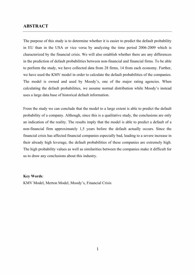
ABSTRACT
The purpose of this study is to determine whether it is easier to predict the default probability
in EU than in the USA or vice versa by analyzing the time period 2006-2009 which is
characterized by the financial crisis. We will also establish whether there are any differences
in the prediction of default probabilities between non-financial and financial firms. To be able
to perform the study, we have collected data from 28 firms, 14 from each economy. Further,
we have used the KMV model in order to calculate the default probabilities of the companies.
The model is owned and used by Moody’s, one of the major rating agencies. When
calculating the default probabilities, we assume normal distribution while Moody’s instead
uses a large data base of historical default information.
From the study we can conclude that the model to a large extent is able to predict the default
probability of a company. Although, since this is a qualitative study, the conclusions are only
an indication of the reality. The results imply that the model is able to predict a default of a
non-financial firm approximately 1,5 years before the default actually occurs. Since the
financial crisis has affected financial companies especially bad, leading to a severe increase in
their already high leverage, the default probabilities of these companies are extremely high.
The high probability values as well as similarities between the companies make it difficult for
us to draw any conclusions about this industry.
Key Words:
KMV Model, Merton Model, Moody’s, Financial Crisis
2
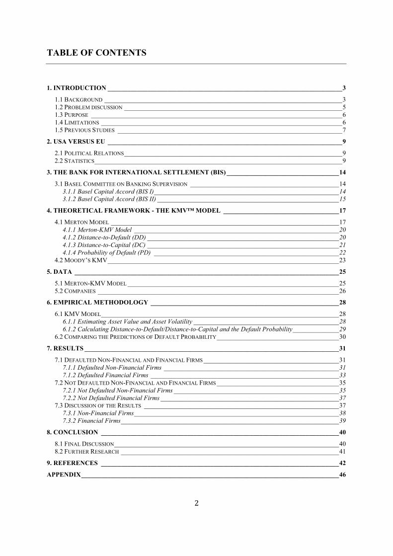
TABLE OF CONTENTS
1. INTRODUCTION _______________________________________________________________________3 1.1 BACKGROUND ________________________________________________________________________3 1.2 PROBLEM DISCUSSION __________________________________________________________________5 1.3 PURPOSE ____________________________________________________________________________6 1.4 LIMITATIONS _________________________________________________________________________6 1.5 PREVIOUS STUDIES ____________________________________________________________________7
2. USA VERSUS EU _______________________________________________________________________9 2.1 POLITICAL RELATIONS__________________________________________________________________9 2.2 STATISTICS___________________________________________________________________________9
3. THE BANK FOR INTERNATIONAL SETTLEMENT (BIS) __________________________________14 3.1 BASEL COMMITTEE ON BANKING SUPERVISION _____________________________________________14
3.1.1 Basel Capital Accord (BIS I)________________________________________________________14 3.1.2 Basel Capital Accord (BIS II) _______________________________________________________15
4. THEORETICAL FRAMEWORK - THE KMV™ MODEL ___________________________________17 4.1 MERTON MODEL _____________________________________________________________________17
4.1.1 Merton-KMV Model ______________________________________________________________20 4.1.2 Distance-to-Default (DD) __________________________________________________________20 4.1.3 Distance-to-Capital (DC) __________________________________________________________21 4.1.4 Probability of Default (PD) ________________________________________________________22
4.2 MOODY’S KMV______________________________________________________________________23 5. DATA ________________________________________________________________________________25
5.1 MERTON-KMV MODEL ________________________________________________________________25 5.2 COMPANIES _________________________________________________________________________26
6. EMPIRICAL METHODOLOGY _________________________________________________________28 6.1 KMV MODEL________________________________________________________________________28
6.1.1 Estimating Asset Value and Asset Volatility ____________________________________________28 6.1.2 Calculating Distance-to-Default/Distance-to-Capital and the Default Probability______________29
6.2 COMPARING THE PREDICTIONS OF DEFAULT PROBABILITY_____________________________________30 7. RESULTS _____________________________________________________________________________31
7.1 DEFAULTED NON-FINANCIAL AND FINANCIAL FIRMS _________________________________________31 7.1.1 Defaulted Non-Financial Firms _____________________________________________________31 7.1.2 Defaulted Financial Firms _________________________________________________________33
7.2 NOT DEFAULTED NON-FINANCIAL AND FINANCIAL FIRMS _____________________________________35 7.2.1 Not Defaulted Non-Financial Firms __________________________________________________35 7.2.2 Not Defaulted Financial Firms ______________________________________________________37
7.3 DISCUSSION OF THE RESULTS ___________________________________________________________37 7.3.1 Non-Financial Firms______________________________________________________________38 7.3.2 Financial Firms__________________________________________________________________39
8. CONCLUSION ________________________________________________________________________40 8.1 FINAL DISCUSSION____________________________________________________________________40 8.2 FURTHER RESEARCH __________________________________________________________________41
9. REFERENCES ________________________________________________________________________42 APPENDIX______________________________________________________________________________46
3
1. INTRODUCTION
1.1 Background
The year of 2006 was the beginning of a worldwide financial crisis, triggered by a collapse of
the housing bubble in the United States.1 The extremely low interest rates during the years
2001-2003 lead to an increased level of lending among the American banks. As a result, the
house prices begun to rise. Banks began lending money even to low income earners, using
subprime loans where the calculations were built on increasing house prices. In order to lower
the risks, banks issued mortgage backed securities (MBS)2 tied to the subprime loans, highly
rated by the rating agencies.
When the house prices started to fall in 2007 the interest rates connected to the subprime
loans increased. Several people who couldn’t handle the increased costs simply handed over
their houses to the banks.3 Since the loans in most cases exceeded the values of houses, this
was a substantial cost for the banks. The subprime loans were soon worthless and thereby
also the bonds tied to them. Banks, investment banks, hedge funds and pension funds all over
the world were affected when forced to write down the values of the bonds. Financial
institutions all over the world were damaged due to a slowdown in the international trade
caused by questioning of their solvency and creditability as well as decreased confidence
among investors.
In March 2008, Bear Sterns, struck by a deep liquidity crisis, was bought out by the
investment bank JP Morgan. In 2008, on September 15, the American investment bank
Lehman Brothers filed for Chapter 114. This was the starting point of a crisis turning out to be
one of the largest in history. The actors in the financial markets choose security above returns.
1Keidel, A. (2008), p 7 2 Mortgage Backed Securities are used in order to derive the risks by splitting them between investors. 3 The risks connected to real estate mortgages in the USA differ from Swedish risks. In the USA, individuals who are unable to fulfil their obligations towards the bank have the possibility of giving the real estate to the bank in exchange of them writing off the liabilities. 4 The US bankruptcy code, defined as reorganization of a company in distress. (Ogden, J. P., Jen, F. C. & O’Connor, P. F. (2002), p 160)
4
Governments and central banks have supported a substantial number of companies and
institutions in terms of fiscal stimulus, monetary policy expansion and institutional bailouts.5
The European banks were immediately affected by the crisis in the US. Due to the close link
between banks and other industries in the European region, the crisis was quickly spread
further in the economies. There are tendencies showing that USA is further into the financial
crisis than Europe. USA has reacted strongly, lowering the interest rates in order to stimulate
the national growth. In Europe on the other hand, the growth seems to develop in a much
slower pace.6 There are economies such as Iceland and Greece almost collapsing. The
inflation has increased explosively in Iceland and the economic recession is severe in both
countries.7
Several banks made the mistake of not holding enough capital in reserve in case of credit
downgrades. BIS II agreements imply that the capital requirements of the banks rise
exponentially due to credit downgrades. The idea of BIS II is therefore to match the capital
requirements with the firms’ ratings while BIS I has an overall requirement of a capital
reserve of 8% regardless the company.8
As argued above, it is of great importance being able to predict the credit risk and the
probability of default among companies. There are several models developed for the purpose
measuring the probability of default, traditional and modern. The traditional models involve
models such as Expert Systems and Neutral Networks (AI) and modern models involve
Reduced Form Models, Actuarial Models, Credit Migration Models and Contingent Claims
Models (Structural Models). Today, the most common models are the Credit Migration
models (Credit Metrics) and the Structural models (KMV).
5 Dagens Industri (http://www.e24.se/business/bank-och-finans/hang-med-i-finanskrisens-alla-svangar_777413.e24) 6 HQ Bank (http://www.hq.se/sv/Strukturerade-produkter/Marknadsinformation/hq-kurslista/USA-vs-Europa/) 7 Islandsbanki (http://www.islandsbanki.is/english/) 8 Moody’s (http://www.moodyskmv.com/cpc06/pres/01_Deloitte.pdf)
5
“Complete realism is clearly unattainable, and the question whether a theory is realistic
enough can be settled only by seeing whether it yields predictions that are good enough for
the purpose in hand or that are better than predictions from alternative theories.” (Friedman,
1953)
This statement was presented by Milton Friedman decades ago but applies well to the current
debate regarding models measuring probability of default. Much of the debate is about
assumptions and theory but relatively little is written about empirical application of the
models. This paper will focus on the empirical performance of one of the models measuring
the default probability, the structural KMV model.
1.2 Problem discussion
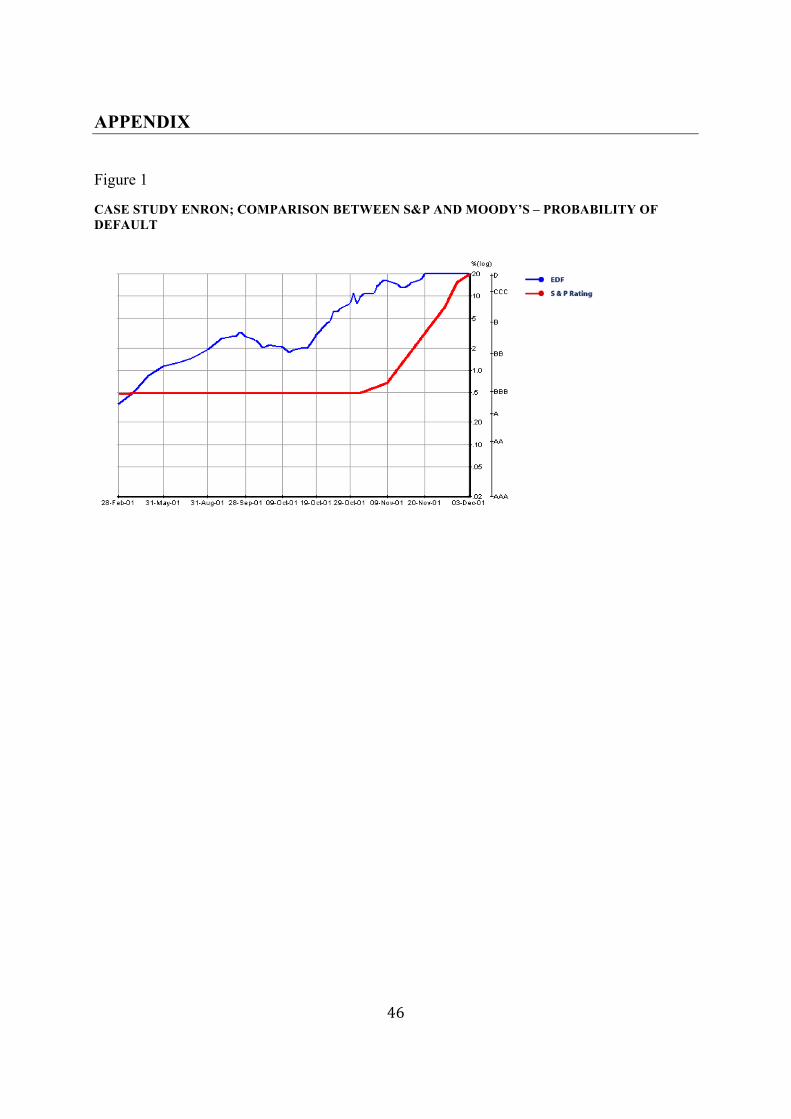
During the financial crisis, rating agencies such as Moody’s, Standard & Poor’s and Fitch
have been criticised for not being able to predict the credit risk of companies appropriately. In
contrast, they have strongly been undervaluing the probability of default. The result has been
that many market participants choose to no longer rely on their ratings.9 The question is how
bad the predictions of the models measuring probability of default actually were. Case studies
show that Moody’s KMV model has been able to predict the default probabilities of
companies earlier than, for example, Standard & Poor’s, see figure 1 in Appendix.10
The financial crisis first started in USA and not until months later the EU was affected. Due
to strong relations and differences between the USA and the EU, we find it interesting to
make a comparison between the economies. There are factors pointing towards a difference in
the ability to predict the default probabilities between the economies but also against, see
further discussion in chapter two. The period during the financial crisis is extremely volatile
and historically important. Many companies have defaulted, both financial and non-financial,
and we therefore find it interesting to analyze this further. We also believe that the difference
in calculating the probability of default of financial and non-financial firms as well as the
“governmental parachutes” of financial institutions, lead to differences in the ability of
predicting the probabilities in between. 9 Worldbank (http://rru.worldbank.org/documents/CrisisResponse/Note8.pdf), p 1 10 Moody’s (http://www.moodyskmv.com/research/files/Enron.pdf)
6
The discussion above leads us to the main question of the thesis:
• Has there been a difference11 in the predictions of the default probabilities of
companies from the USA and EU during the financial crisis?
We further want to answer the question:
• Has there been a difference in the predictions of the default probability of financial
and non-financial firms?
1.3 Purpose
The purpose of the thesis is to examine whether the predictions of default probabilities of
companies in EU have been more accurate than the ones of American companies or vice
versa. The time period which is analyzed in the study is the years between 2006 and 2009.
Further, we will use the structural KMV model in order to perform the study. The study will
be qualitative, using 28 companies, 14 from each of the economies. Since both financial and
non-financial firms will be included in the analysis, another purpose will be to determine
which companies’ predictions of default probabilities are the most accurate.
1.4 Limitations
In the thesis we have decided to limit the study to the economies EU and USA and exclude
other large economies from the study in order to limit the analysis. Since the analysis demand
several parameters and observations, we will focus on a limited number of companies (28).
To be able to analyze the economies as reliable as possible, we have chosen companies from
several industries12 and countries13 as well as both financial and non-financial companies.
In order to fully determine the accuracy of the model we will analyze both defaulted and not
defaulted companies. In this paper we will define default as the point where the market value
of assets is equal to or less than the total liabilities. This definition was first developed in a
11 “Easier to predict the default probabilities in one of the economies than in the other” 12 Holding, Motor Vehicle, Leisure & Media, Telecommunication, Transport, Clothing & Consumer Goods, Metal, High Tech and Financial firms 13 USA, Denmark, France, Germany, Hungary, Iceland, Luxembourg, Netherlands, Sweden and Switzerland. Companies from Iceland and Switzerland are also included in order to capture the volatility of the Icelandic market as well as information about large financial institutions (UBS and Credit Suisse).
7
research made by Moody’s. The market value of assets subtracted by the default point is also
defined as the net worth of a company.14 Since the model requires market data, we will only
analyze stock-noted companies.
There are several different models measuring companies’ probability of default. Further
rating agencies have been strongly criticized during the financial crisis. We wanted to focus
on a modern model, used by rating agencies and investment banks today. Therefore, we chose
to use the KMV model, a model used by the rating institute Moody’s today.
1.5 Previous Studies
Several studies have been performed on the KMV model, primarily in order to examine the
accuracy of the model and finding models to make improvements of it. Many of the studies
can be found on Moody’s website. The KMV model was summarized by Crosbie and Bohn
after making some modifications on the assumptions. They applied the model in order to
calculate the market value and volatility of the firm’s asset from equity in order to improve
the accuracy of the Distance-to-Default.15 Kealhofer and Kurbat argue that Moody’s KMV
model captures more information and react quicker compared to traditional rating agencies.16
Further information about improvements made regarding the KMV model will be discussed
in chapter four. Several scholars have also been interested in examining the accuracy of the
model.17
Korablev and Dwyer validate the performance of Moody’s KMV EDF™ (Expected Default
Frequency) model during the period 1996-2006. They compare the accuracy of the model
predictions in three regions; North America, Europe and Asia. They conclude that the KMV
model works well in all of the three regions.18 Korablev and Qu examine the performance of
Moody’s KMV EDF™ model during the financial crisis. In the study they compare the
performance of the model during 2007-2009 and 1996-2006, using two primary samples;
North American non-financial firms and global financial firms. They find that the model
14 Crosbie, P.J. & Bohn, J.R. (2003), p 7 15 Crosbie, P. J & Bohn J.R. (2003) 16 Kealhofer, S. & Kurbat, M. (2000) 17 Bharath, S.T. & Shumway, T. (2004) 18 Korablev, I. & Dwyer, D.W. (2007)

8
gives good predictions during the financial crisis, providing warning signals a few years
before the actual default event.19
19 Korablev, I. & Qu, S. (2009)

9
2. USA VERSUS EU
This part of the thesis will focus on the relations and the differences between the USA and the
EU indicating the level of interest in comparing the economies.
2.1 Political Relations
In 1953, diplomatic relations were established between the USA and Europe. Although, this
cooperation wasn’t formally set up until 1990 when the economies formed the Transatlantic
Declaration. The New Transatlantic Agenda has been the foundation of the relationship since
1995 including meetings between USA and EU leaders as well as technical work at expert
level. In 2007, the Transatlantic Economic Council (TEC) was founded in order to boost the
economy. Areas covered by the TEC cooperation are among others secure trade, investments,
financial markets as well as innovation and technology.20 Any disputes between the
economies regarding the trade in between are settled through the World Trade Organisation
(WTO), established in 1995. In 2008, 153 countries were members of the organisation, all 27
EU member states included.21
2.2 Statistics
Together, USA and EU stand for the largest investment relationship and bilateral trade in the
world. The transatlantic trade has during the last years followed a steady upward sloping
trend. The economies are together responsible for more than half of the world GDP and
account for almost 40% of the world trade, being each other’s main trading partners (2007).22
Apart from the trade, investments between the economies are also important. In terms of
Foreign Direct Investments, the economies are each other’s most important sources.23 The
table below shows the amounts traded between the economies.
20 European Commission (http://ec.europa.eu/enterprise/policies/international/cooperating-governments/usa/transatlantic-economic-council/index_en.htm#h2-areas-of-cooperation) 21 European Commission (http://ec.europa.eu/trade/creating-opportunities/bilateral-relations/countries/united-states/index_en.htm) 22 European Commission (http://ec.europa.eu/external_relations/us/index_en.htm) 23 European Commission (http://ec.europa.eu/external_relations/us/economic_en.htm)
10
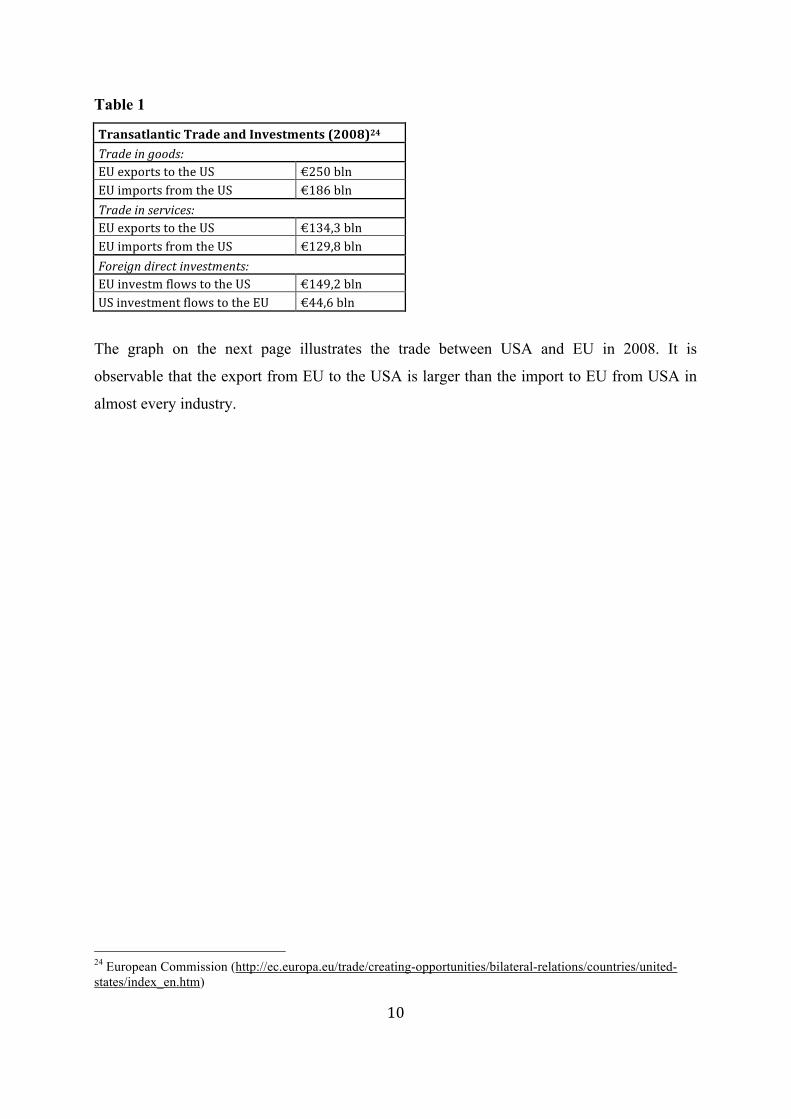
Table 1
TransatlanticTradeandInvestments(2008)24
Tradeingoods:EUexportstotheUS €250blnEUimportsfromtheUS €186blnTradeinservices:EUexportstotheUS €134,3blnEUimportsfromtheUS €129,8blnForeigndirectinvestments:EUinvestmflowstotheUS €149,2blnUSinvestmentflowstotheEU €44,6bln
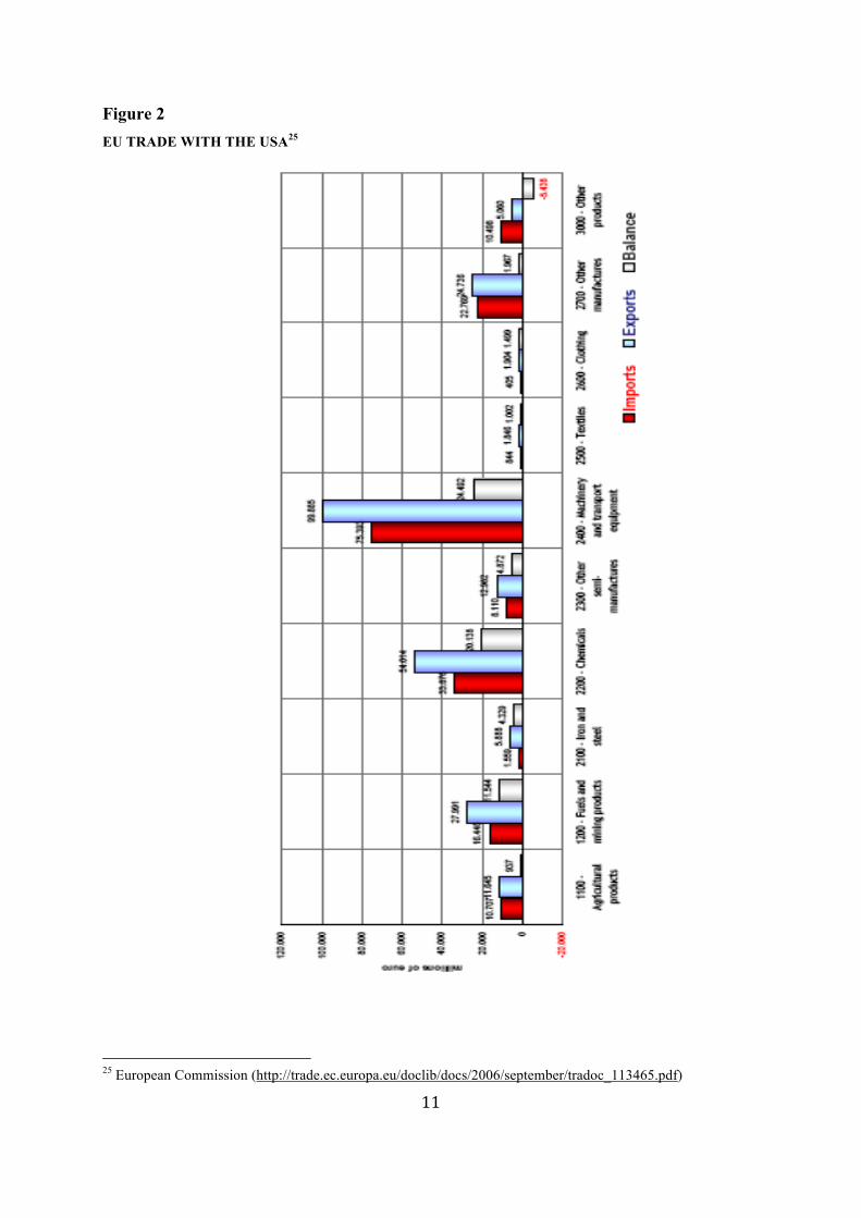
The graph on the next page illustrates the trade between USA and EU in 2008. It is
observable that the export from EU to the USA is larger than the import to EU from USA in
almost every industry.
24 European Commission (http://ec.europa.eu/trade/creating-opportunities/bilateral-relations/countries/united-states/index_en.htm)
11
Figure 2 EU TRADE WITH THE USA25
25 European Commission (http://trade.ec.europa.eu/doclib/docs/2006/september/tradoc_113465.pdf)
12
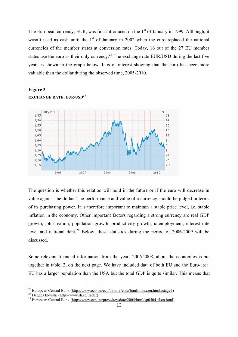
The European currency, EUR, was first introduced on the 1st of January in 1999. Although, it
wasn’t used as cash until the 1st of January in 2002 when the euro replaced the national
currencies of the member states at conversion rates. Today, 16 out of the 27 EU member
states use the euro as their only currency.26 The exchange rate EUR/USD during the last five
years is shown in the graph below. It is of interest showing that the euro has been more
valuable than the dollar during the observed time, 2005-2010.
Figure 3 EXCHANGE RATE, EUR/USD27
The question is whether this relation will hold in the future or if the euro will decrease in
value against the dollar. The performance and value of a currency should be judged in terms
of its purchasing power. It is therefore important to maintain a stable price level, i.e. stable
inflation in the economy. Other important factors regarding a strong currency are real GDP
growth, job creation, population growth, productivity growth, unemployment, interest rate
level and national debt.28 Below, these statistics during the period of 2006-2009 will be
discussed.
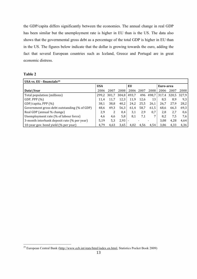
Some relevant financial information from the years 2006-2008, about the economies is put
together in table, 2, on the next page. We have included data of both EU and the Euro-area.
EU has a larger population than the USA but the total GDP is quite similar. This means that
26 European Central Bank (http://www.ecb.int/ecb/history/emu/html/index.en.html#stage2) 27 Dagens Industri (http://www.di.se/trader) 28 European Central Bank (http://www.ecb.int/press/key/date/2005/html/sp050415.en.html)
13
the GDP/capita differs significantly between the economies. The annual change in real GDP
has been similar but the unemployment rate is higher in EU than is the US. The data also
shows that the governmental gross debt as a percentage of the total GDP is higher in EU than
in the US. The figures below indicate that the dollar is growing towards the euro, adding the
fact that several European countries such as Iceland, Greece and Portugal are in great
economic distress.
Table 2
USAvs.EUfinancials29 USAEUEuroareaData\Year 2006 2007 2008 2006 2007 2008 2006 2007 2008Totalpopulation(millions) 299,2 301,7 304,8 493,7 496 498,7 317,4 320,5 327,9GDP,PPP(%) 11,4 11,7 12,3 11,9 12,6 13 8,5 8,9 9,3GDP/capita,PPP(%) 38,1 38,8 40,2 24,2 25,5 26,1 26,7 27,9 28,2Governmentgrossdebtoutstanding(%ofGDP) 48,6 49,3 56,3 61,4 58,7 61,5 68,6 66,3 69,3RealGDP(annual%change) 2,9 2 0,4 3,1 2,9 0,7 2,8 2,7 0,6Unemploymentrate(%oflabourforce) 4,6 4,6 5,8 8,1 7,1 7 8,2 7,5 7,63‐monthinterbankdepositrate(%peryear) 5,19 5,3 2,93 ‐ ‐ ‐ 3,08 4,28 4,6410‐yeargov.bondyield(%peryear) 4,79 4,63 3,65 4,02 4,56 4,54 3,86 4,33 4,36
29 European Central Bank (http://www.ecb.int/stats/html/index.en.html, Statistics Pocket Book 2009)
14
3. THE BANK FOR INTERNATIONAL SETTLEMENT (BIS)
The Bank for International Settlement (BIS) is an international organisation and a bank for
central banks, founded in May, 1930. Its main tasks are to be a counterparty for international
central banks in their financial transactions, a midpoint for economic and monetary research,
an agent in connection with international financial operations and a platform for promotion of
discussion and policy analysis among the central banks.30
3.1 Basel Committee on Banking Supervision
The Basel committee was established in 1974 and consists of central banks from the largest
industrialized countries worldwide31. The committee serves as a regular cooperation on
banking supervisory and in order to improve the quality of it. Further, the committee works
for stability in the economy and one task of the committee is to maintain the international
standards on capital adequacy, known as BIS I (1998) and BIS II (2008).32 The Basel
committee is a part of BIS, but BIS is not a participant in the decisions that are taken within
the committee.33
3.1.1 Basel Capital Accord (BIS I)
Credit risk management and measuring the probability of default of a company is a complex
process which is obstructed primarily by the correlation in credit events. This means that the
uncertainty underlying the probability of default is cyclical due to the fact that a recession will
lead to a cluster of default events. The existence of the default correlation is recognized by
BIS regulations.34
30 Bank of International Settlements (http://www.bis.org/about/index.htm) 31 Argentina, Australia, Belgium, Brazil, Canada, China, France, Germany, Hong Kong SAR, India, Indonesia, Italy, Japan, Korea, Luxembourg, Mexico, the Netherlands, Russia, Saudi Arabia, Singapore, South Africa, Spain, Sweden, Switzerland, Turkey, the United Kingdom and the United States 32 Bank of International Settlements (http://bis.org/bcbs/index.htm#Consultative_Group) 33 Bank of International Settlements (http://www.bis.org/about/index.htm) 34 Dwyer, D. W. (2006), p 3
15
The BIS I framework contains of standards for capital requirements saying that financial
institutions must hold at least 8% of its assets as a reserve against unexpected losses. The
implementation of BIS I was supported by the G-10 countries35.36
3.1.2 Basel Capital Accord (BIS II)
The capital accord, BIS II, is a development of the BIS I framework and was first introduced
in 2007 and further implemented in 2008-2009.37 While BIS I focuses on a single risk
measure and states that all loans should be treated equally, BIS II is more focused on risk
sensitivity. BIS II takes the financial institutions’ internal methodologies, supervisory review
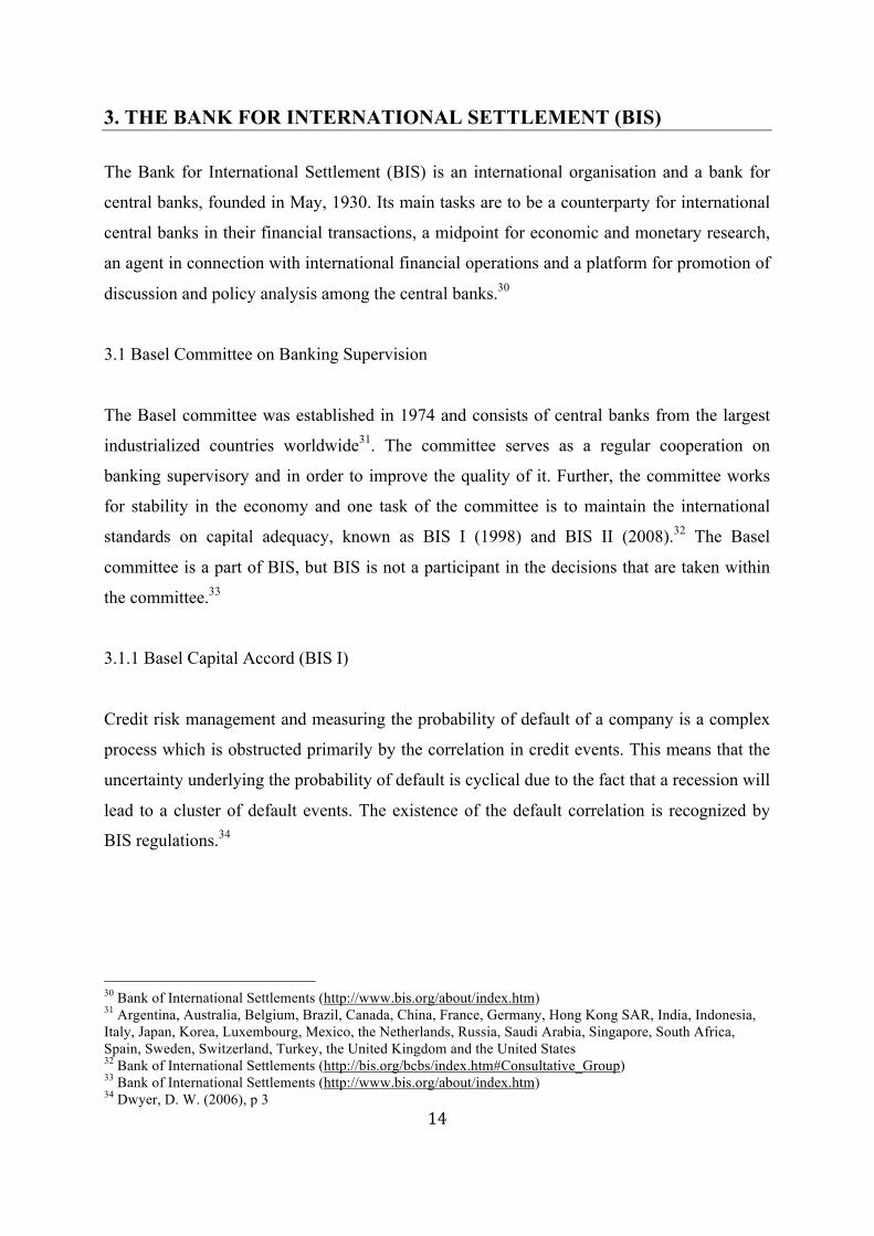
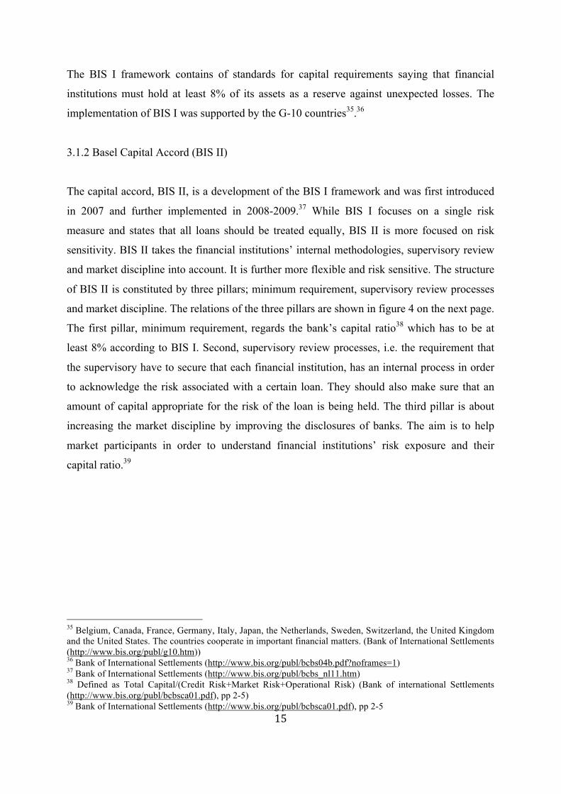
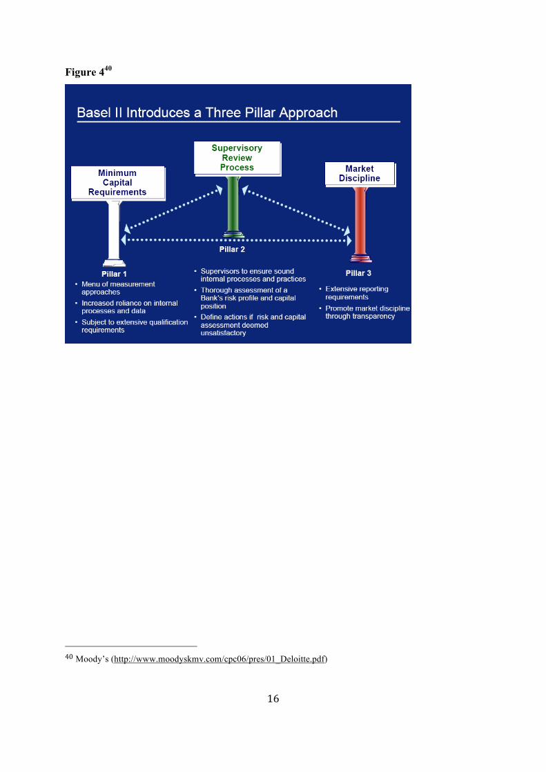
and market discipline into account. It is further more flexible and risk sensitive. The structure
of BIS II is constituted by three pillars; minimum requirement, supervisory review processes
and market discipline. The relations of the three pillars are shown in figure 4 on the next page.
The first pillar, minimum requirement, regards the bank’s capital ratio38 which has to be at
least 8% according to BIS I. Second, supervisory review processes, i.e. the requirement that
the supervisory have to secure that each financial institution, has an internal process in order
to acknowledge the risk associated with a certain loan. They should also make sure that an
amount of capital appropriate for the risk of the loan is being held. The third pillar is about
increasing the market discipline by improving the disclosures of banks. The aim is to help
market participants in order to understand financial institutions’ risk exposure and their
capital ratio.39
35 Belgium, Canada, France, Germany, Italy, Japan, the Netherlands, Sweden, Switzerland, the United Kingdom and the United States. The countries cooperate in important financial matters. (Bank of International Settlements (http://www.bis.org/publ/g10.htm)) 36 Bank of International Settlements (http://www.bis.org/publ/bcbs04b.pdf?noframes=1) 37 Bank of International Settlements (http://www.bis.org/publ/bcbs_nl11.htm) 38 Defined as Total Capital/(Credit Risk+Market Risk+Operational Risk) (Bank of international Settlements (http://www.bis.org/publ/bcbsca01.pdf), pp 2-5) 39 Bank of International Settlements (http://www.bis.org/publ/bcbsca01.pdf), pp 2-5
16
Figure 440
40Moody’s (http://www.moodyskmv.com/cpc06/pres/01_Deloitte.pdf)
17
4. THEORETICAL FRAMEWORK - THE KMV™ MODEL
In this paper we will use the modern credit risk model, KMV™, in order to determine the
default probability of 28 companies. The model has a structural form, meaning that it has the
characteristics of describing the internal debt structure of a company where default is a
consequence of an internal event.41 Default risk is defined as the uncertainty surrounding a
firm’s ability to amortize the debts and fulfil its obligations.42
The KMV model has its origin in the Merton model, developed by Robert Merton in 1974.
The Merton model uses an extended version of the Black and Scholes framework on option
pricing theory in the default prediction of a firm. Later, the Merton model was further
developed by the KMV Corporation. The KMV-Merton model is based upon Merton’s
assumption that a firm’s equity is a European call option on the underlying assets.43 Further,
the founders of the KMV model, Oldrich Vasicek and Stephen Kealhofer, extended the Black
and Scholes framework to the VK-model, assuming that a firm’s equity is a perpetual barrier
option on the underlying value of the firm’s asset in a time, T. In 2002, the KMV Corporation
was bought by the rating agency Moody’s in order to use the KMV model as well as the
competence of the company. Today, the model is known as Moody’s KMV model.44
4.1 Merton Model
When defining the equity of a company as a European call option on the asset of the
company, the model uses the time to maturity, T, and the strike price, X, which is equal to the
repayable debt of the firm. In the development of the Black-Scholes formula, Merton made
several assumptions;
1. There is a perfect market where there are no transactions cost or taxes. There are also
a sufficient number of investors with comparable wealth, no limitations for the
investors when selling and buying assets and short-sales are allowed. The interest rate
is constant and known. 41 Saunders, A. & Allen, L. (2002), p 49 42 Crosbie, P.J. & Bohn, J.R. (2003), p 5 43 Delianedis, G & Geske, R (1998), p 3 44 Crosbie, P.J. & Bohn, J.R. (2003), p 10
18
2. The trading of assets is continuous over time.
3. The value of the firm is invariant with its capital structure, which means that the
company is founded by a single class of equity and a single class of debt (Miller-
Modigliani).
4. There is only one homogeneous class of bonds issued by the firm, maturing within the
period T. The firm is obligated to pay back the bond to the bondholder at T.
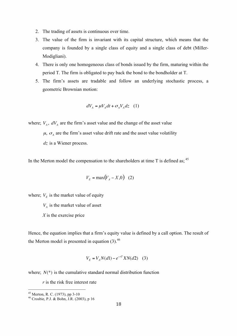
5. The firm’s assets are tradable and follow an underlying stochastic process, a
geometric Brownian motion:
(1)
where; , are the firm’s asset value and the change of the asset value
, are the firm’s asset value drift rate and the asset value volatility
is a Wiener process.
In the Merton model the compensation to the shareholders at time T is defined as; 45
(2)
where; is the market value of equity
is the market value of asset
X is the exercise price
Hence, the equation implies that a firm’s equity value is defined by a call option. The result of
the Merton model is presented in equation (3).46
(3)
where; is the cumulative standard normal distribution function
r is the risk free interest rate 45 Merton, R. C. (1973), pp 3-10 46 Crosbie, P.J. & Bohn, J.R. (2003), p 16
19
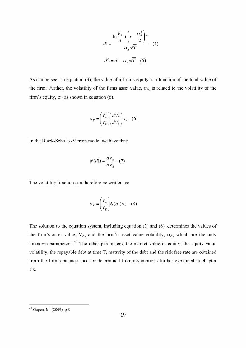
(4)
(5)
As can be seen in equation (3), the value of a firm’s equity is a function of the total value of
the firm. Further, the volatility of the firms asset value, σA, is related to the volatility of the
firm’s equity, σE, as shown in equation (6).
(6)
In the Black-Scholes-Merton model we have that:
(7)
The volatility function can therefore be written as:
(8)
The solution to the equation system, including equation (3) and (8), determines the values of
the firm’s asset value, VA, and the firm’s asset value volatility, σA, which are the only
unknown parameters. 47 The other parameters, the market value of equity, the equity value
volatility, the repayable debt at time T, maturity of the debt and the risk free rate are obtained
from the firm’s balance sheet or determined from assumptions further explained in chapter
six.
47 Gapen, M. (2009), p 8
20
4.1.1 Merton-KMV Model
This model is based upon Merton’s assumptions that the equity is a call option on a firm’s
asset value. Further, according to the Merton model, asset value and asset value volatility are
determined by Black and Scholes option pricing based approach. Further, the KMV model
uses the measures distance-to-default and distance-to-capital when determining the default
probability of non-financial firms and financial firms respectively.
Since we include different countries and industries in the study, it is of great importance that
the model captures the particular differences regarding this information. According to Crosbie
and Bohn, the business risk is measured by the asset volatility which varies between
industries and across countries. They further believe that countries wealth is captured in the
equity and asset values of the companies. Since asset volatility as well as asset and equity
values are included in the model, it is assumed to be applicable when comparing different
industries and countries.48
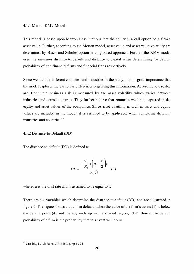
4.1.2 Distance-to-Default (DD)
The distance-to-default (DD) is defined as:
(9)
where; µ is the drift rate and is assumed to be equal to r.
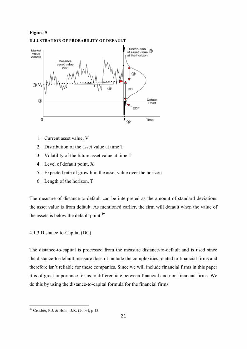
There are six variables which determine the distance-to-default (DD) and are illustrated in
figure 5. The figure shows that a firm defaults when the value of the firm’s assets (1) is below
the default point (4) and thereby ends up in the shaded region, EDF. Hence, the default
probability of a firm is the probability that this event will occur.
48 Crosbie, P.J. & Bohn, J.R. (2003), pp 18-21
21
Figure 5 ILLUSTRATION OF PROBABILITY OF DEFAULT
1. Current asset value, Vt
2. Distribution of the asset value at time T
3. Volatility of the future asset value at time T
4. Level of default point, X
5. Expected rate of growth in the asset value over the horizon
6. Length of the horizon, T
The measure of distance-to-default can be interpreted as the amount of standard deviations
the asset value is from default. As mentioned earlier, the firm will default when the value of
the assets is below the default point.49
4.1.3 Distance-to-Capital (DC)
The distance-to-capital is processed from the measure distance-to-default and is used since
the distance-to-default measure doesn’t include the complexities related to financial firms and
therefore isn’t reliable for these companies. Since we will include financial firms in this paper
it is of great importance for us to differentiate between financial and non-financial firms. We
do this by using the distance-to-capital formula for the financial firms.
49 Crosbie, P.J. & Bohn, J.R. (2003), p 13
22
Both USA and EU are members of BIS and the Basel Committee of Banking Supervision. It
is therefore relevant to use their requirements in our calculations. Since we are not able to
evaluate the companies’ every single debt as BIS II (2008) implies, we will instead use the
requirements of BIS I (1988). BIS I requires that a financial institution must hold a minimum
capital amount equal to 8% of its risky assets. To be able to identify weak banks from strong
and find good solutions for those, several financial institutions have implemented prompt
corrective action (PCA). PCA is a number of rules and actions which need to be used if the
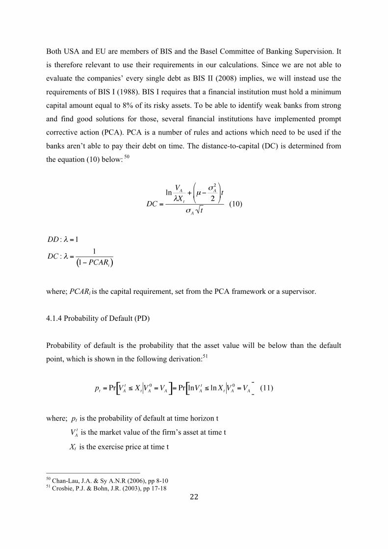
banks aren’t able to pay their debt on time. The distance-to-capital (DC) is determined from
the equation (10) below: 50
(10)
where; PCARi is the capital requirement, set from the PCA framework or a supervisor.
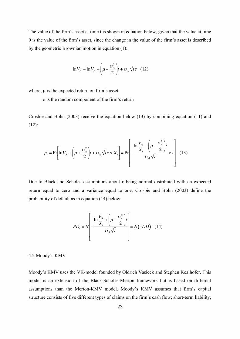
4.1.4 Probability of Default (PD)
Probability of default is the probability that the asset value will be below than the default
point, which is shown in the following derivation:51
(11)
where; pt is the probability of default at time horizon t
is the market value of the firm’s asset at time t
Xt is the exercise price at time t
50 Chan-Lau, J.A. & Sy A.N.R (2006), pp 8-10 51 Crosbie, P.J. & Bohn, J.R. (2003), pp 17-18
23
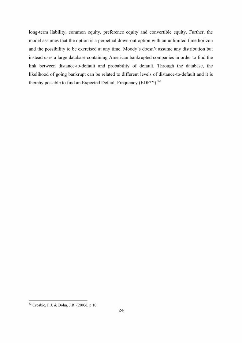
The value of the firm’s asset at time t is shown in equation below, given that the value at time
0 is the value of the firm’s asset, since the change in the value of the firm’s asset is described
by the geometric Brownian motion in equation (1):
(12)
where; µ is the expected return on firm’s asset
ε is the random component of the firm’s return
Crosbie and Bohn (2003) receive the equation below (13) by combining equation (11) and
(12):
(13)
Due to Black and Scholes assumptions about ε being normal distributed with an expected
return equal to zero and a variance equal to one, Crosbie and Bohn (2003) define the
probability of default as in equation (14) below:
(14)
4.2 Moody’s KMV
Moody’s KMV uses the VK-model founded by Oldrich Vasicek and Stephen Kealhofer. This
model is an extension of the Black-Scholes-Merton framework but is based on different
assumptions than the Merton-KMV model. Moody’s KMV assumes that firm’s capital
structure consists of five different types of claims on the firm’s cash flow; short-term liability,
24
long-term liability, common equity, preference equity and convertible equity. Further, the
model assumes that the option is a perpetual down-out option with an unlimited time horizon
and the possibility to be exercised at any time. Moody’s doesn’t assume any distribution but
instead uses a large database containing American bankrupted companies in order to find the
link between distance-to-default and probability of default. Through the database, the
likelihood of going bankrupt can be related to different levels of distance-to-default and it is
thereby possible to find an Expected Default Frequency (EDF™).52
52 Crosbie, P.J. & Bohn, J.R. (2003), p 10
25
5. DATA
5.1 Merton-KMV Model
In this part of the paper, we will present the data collected in order to perform the study. The
data includes corporate stock prices, short and long term debt, number of shares outstanding
as well as the interest rates of 3-month Treasury bills53. All data except the debt was found in
the DataStream database54 and consists of daily observations from the period 2006-01-01 to
2009-12-31. The debt values were collected from the companies’ balance sheets, using yearly
observations. Note that the usage of yearly data slightly will decrease the reliability of the
model. In order to make a relevant comparison between the economies we have chosen 14
companies from the USA and 14 from the EU. Twelve of the companies used in the study
have defaulted during the period and 16 are still running. The defaulted companies included
in our study are chosen based on default dates as late as possible during the period, in order to
analyze a large part of the financial crisis.
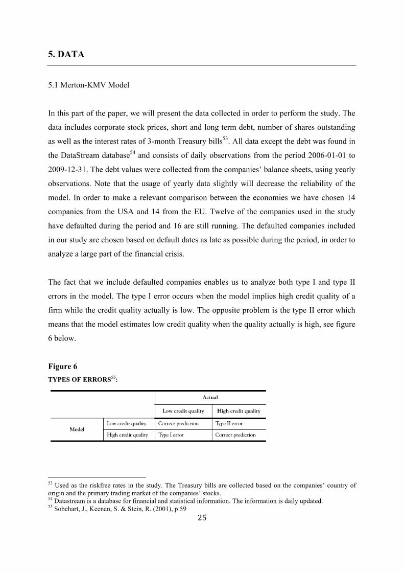
The fact that we include defaulted companies enables us to analyze both type I and type II
errors in the model. The type I error occurs when the model implies high credit quality of a
firm while the credit quality actually is low. The opposite problem is the type II error which
means that the model estimates low credit quality when the quality actually is high, see figure
6 below.
Figure 6 TYPES OF ERRORS55:
53 Used as the riskfree rates in the study. The Treasury bills are collected based on the companies’ country of origin and the primary trading market of the companies’ stocks. 54 Datastream is a database for financial and statistical information. The information is daily updated. 55 Sobehart, J., Keenan, S. & Stein, R. (2001), p 59
26
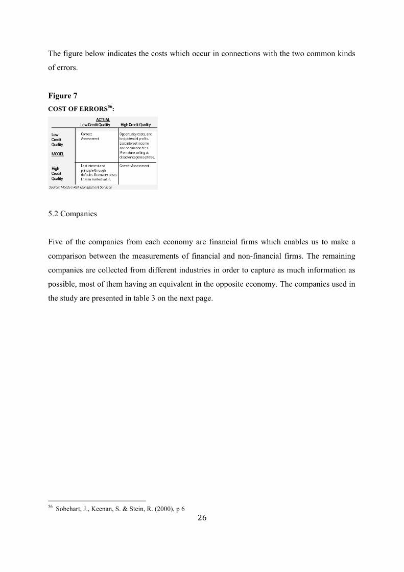
The figure below indicates the costs which occur in connections with the two common kinds
of errors.
Figure 7 COST OF ERRORS56:
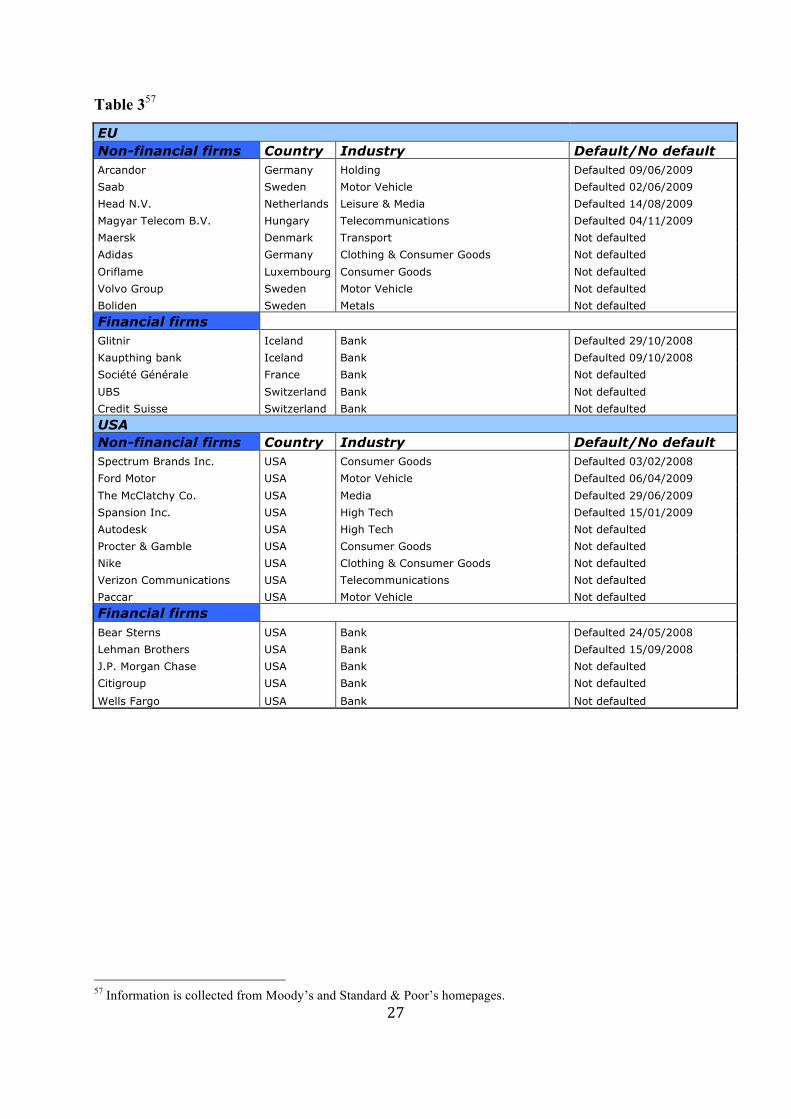
5.2 Companies
Five of the companies from each economy are financial firms which enables us to make a
comparison between the measurements of financial and non-financial firms. The remaining
companies are collected from different industries in order to capture as much information as
possible, most of them having an equivalent in the opposite economy. The companies used in
the study are presented in table 3 on the next page.
56 Sobehart, J., Keenan, S. & Stein, R. (2000), p 6
27
Table 357
EU Non-financial firms Country Industry Default/No default Arcandor Germany Holding Defaulted 09/06/2009
Saab Sweden Motor Vehicle Defaulted 02/06/2009
Head N.V. Netherlands Leisure & Media Defaulted 14/08/2009
Magyar Telecom B.V. Hungary Telecommunications Defaulted 04/11/2009
Maersk Denmark Transport Not defaulted
Adidas Germany Clothing & Consumer Goods Not defaulted
Oriflame Luxembourg Consumer Goods Not defaulted
Volvo Group Sweden Motor Vehicle Not defaulted
Boliden Sweden Metals Not defaulted
Financial firms
Glitnir Iceland Bank Defaulted 29/10/2008
Kaupthing bank Iceland Bank Defaulted 09/10/2008
Société Générale France Bank Not defaulted
UBS Switzerland Bank Not defaulted
Credit Suisse Switzerland Bank Not defaulted
USA Non-financial firms Country Industry Default/No default Spectrum Brands Inc. USA Consumer Goods Defaulted 03/02/2008
Ford Motor USA Motor Vehicle Defaulted 06/04/2009
The McClatchy Co. USA Media Defaulted 29/06/2009
Spansion Inc. USA High Tech Defaulted 15/01/2009
Autodesk USA High Tech Not defaulted
Procter & Gamble USA Consumer Goods Not defaulted
Nike USA Clothing & Consumer Goods Not defaulted
Verizon Communications USA Telecommunications Not defaulted
Paccar USA Motor Vehicle Not defaulted
Financial firms Bear Sterns USA Bank Defaulted 24/05/2008
Lehman Brothers USA Bank Defaulted 15/09/2008
J.P. Morgan Chase USA Bank Not defaulted
Citigroup USA Bank Not defaulted
Wells Fargo USA Bank Not defaulted
57 Information is collected from Moody’s and Standard & Poor’s homepages.
28
6. EMPIRICAL METHODOLOGY
As mentioned in the part about BIS II, the methodology for assigning credit assessment is
important for all companies. In this part of the paper the KMV model will be empirically
applied, using real data in order to compare the accuracy of the model predictions in the USA
and the EU. In order to perform the comparison, we will separate financial from non-financial
firms and defaulted companies from companies not yet defaulted. Further, all of the data we
need isn’t directly observable. Therefore, we have made a few simplifications and
assumptions when implementing the model. This is further explained in chapter four.
6.1 KMV Model
In this part we will derive and determine the three parameters necessary for measuring the
default probability; the market value of assets, asset value volatility and liabilities. In order to
find the parameters both financial statements, book values of the companies’ debt, market
prices of the companies’ equity as well as subjective valuations of the firms’ prospects and
risks are important. The first two parameters, value of assets and asset value volatility, are
unknown and the third parameter, liabilities, is observable but it is discussed what should be
included in it. The liability parameter and the determination of the drift rate and the time to
maturity will be discussed further down in this part.
6.1.1 Estimating Asset Value and Asset Volatility
The Merton-KMV model uses an option based approach when determining the value of assets
and the asset volatility. The equity can be used as a call option on the underlying assets of the
company where the strike price equals the book value of the liabilities. To be able to solve for
the parameters, asset value and asset value volatility, two equations will be used. First we use
the relationship between the market value of a firm’s equity and the market value of its asset
which is explained in equation (3). The equity value is calculated from multiplying the
number of shares outstanding and the stock price of the firm. The second equation which is
explained in equation (8), also defined as σE = f(σA), explains the relationship between the
volatility of the firm’s assets and the volatility of firm’s equity. In order to solve these
29
equations we first need to determine the values of the liabilities, drift rate and time to
maturity.
As was mentioned in the theoretical part, the Merton-KMV model is assumed to be normal
distributed due to the lack of Moody’s database. This assumption implicates several
drawbacks of the result. While the Merton-KMV model sets a constant, the liabilities, to be
equal to the default point, Moody’s default point is a variable. Besides, in our case, the
liabilities are retrieved from the financial statement and are therefore historical and out of
date. Further it has been discussed whether to use the net short-term liabilities or the total
amount of short-term liabilities since different liabilities have different time to maturities.58
Moody’s use the total value of short-term and half of the long-term liabilities of a firm and
this is also the definition we will use in the study.59 Further, the maturity of the debt is
supposed to match the purpose of the study and is therefore assumed to equal one year in this
paper since this is the time horizon of the KMV model. The normality assumption also results
in a loss of extreme observations since its tails aren’t as wide as the ones of the actual
distribution.60 The drift rate is assumed to be equal to the risk-free rate. As mentioned in the
data section, 3-month treasury bills are used in order to determine the risk free interest rate.
The parameters asset value and the asset value volatility are optimized by using Excel and
VBA61.
6.1.2 Calculating Distance-to-Default/Distance-to-Capital and the Default Probability
Using the estimated parameters, we use equation 9 in order to calculate the distance-to-
default of the non-financial firms and equation 10 to calculate the distance-to-capital of the
financial firms. The last step is to calculate the default probabilities, using equation 14, of all
companies included in the study. The results are discussed in part seven below.
58 Saunders, A. & Allen L. (2002), p 51 59 Crosbie, P.J. & Bohn, J.R. (2003), p 7 60 Crosbie, P.J. & Bohn, J.R. (2003), p 18 61 Visual Basic for Applications
30
6.2 Comparing the Predictions of Default Probability
When analyzing the type I error (using companies already defaulted), we will compare the
differences in probability of default between the economies eighteen, twelve and six months
before the actual default event. The type II error (using companies not defaulted), will be
analyzed by observing the predictions of the companies in December 2009, looking at the
most relevant key ratios of the companies. The key ratios used in the analysis are debt to
equity62, net margin63 and solvency64.
A high debt to equity ratio implies that the company uses a large amount of debt in the
financing of its growth which might lead to volatile earnings and high interest expenses. To a
certain rate, it might generate more earnings if the return from investing the borrowed capital
is greater than the cost of the debt. The debt to equity ratio is especially relevant in our
analysis since the parameter “liabilities” has a great impact on the default probabilities. This
value can generally be higher in, for example, a financial firm since this industry is more
stable than for example the high technological industry is. This depends on the level of asset
volatility within the industry.65 Further, a company in a mature business with a strong and
stable cash flow is generally able to manage a low net worth in a better way than a company
in an immature business with a low/weak cash flow.66
62 Defined as Total Liabilities/Shareholders Equity and measures a company’s financial leverage. Describes what portion of debt and equity the company uses in order to finance its assets. What is defined as a high D/E ratio depends on the industry. Capital-intensive industries have D/E-ratios above 2 while less capital-intense industries require ratios below 0,5. (Investopedia.com) 63 Defined as Net Profit/Revenue where Net Profit=Revenue-COGS-Operating Expenses-Interest and Taxes. Measures the percentage of the earned money are translated into profits. (Investopedia.com) 64 Defined as (After Tax Net Profit+Depreciation)/(Long Term Liabilities+Short Term Liabilities) and measures a company’s ability to meet its long term obligations. The level of acceptance depends on the industry but generally a solvency ratio higher than 0,2 is considered good enough. A high solvency ratio implies a low probability of default and vice versa. (Investopedia.com) 65 Crosbie, P.J. & Bohn, J.R. (2003), p 9 66 Investopedia.com
31
7. RESULTS
In the study we have included a total amount of 28 companies, both financial and non-
financial. 14 companies are American and an equal number of companies are from the EU. In
this part of the thesis we will present and discuss our estimated values of the default
probabilities, starting with the companies which have defaulted during the time period and
thereafter present and discuss the data about the remaining (non-defaulted) companies.
7.1 Defaulted Non-Financial and Financial Firms
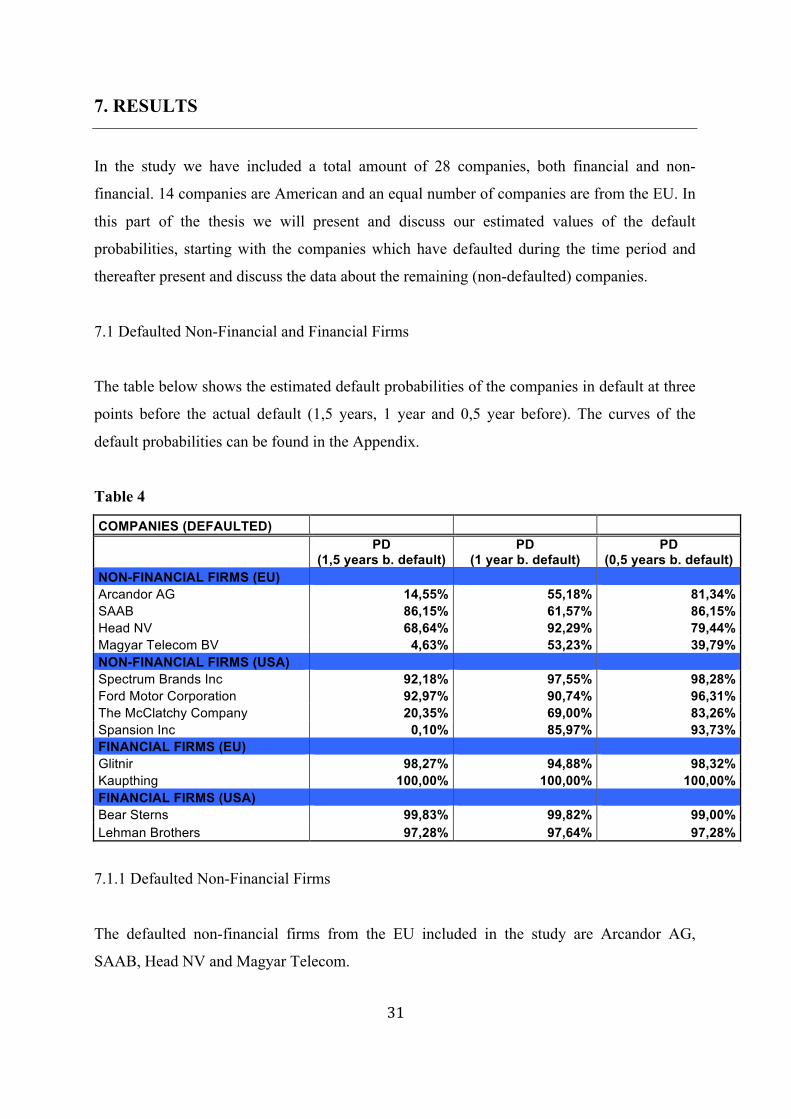
The table below shows the estimated default probabilities of the companies in default at three
points before the actual default (1,5 years, 1 year and 0,5 year before). The curves of the
default probabilities can be found in the Appendix.
Table 4
COMPANIES (DEFAULTED)
PD
(1,5 years b. default) PD
(1 year b. default) PD
(0,5 years b. default) NON-FINANCIAL FIRMS (EU) Arcandor AG 14,55% 55,18% 81,34% SAAB 86,15% 61,57% 86,15% Head NV 68,64% 92,29% 79,44% Magyar Telecom BV 4,63% 53,23% 39,79% NON-FINANCIAL FIRMS (USA) Spectrum Brands Inc 92,18% 97,55% 98,28% Ford Motor Corporation 92,97% 90,74% 96,31% The McClatchy Company 20,35% 69,00% 83,26% Spansion Inc 0,10% 85,97% 93,73% FINANCIAL FIRMS (EU) Glitnir 98,27% 94,88% 98,32% Kaupthing 100,00% 100,00% 100,00% FINANCIAL FIRMS (USA) Bear Sterns 99,83% 99,82% 99,00% Lehman Brothers 97,28% 97,64% 97,28%
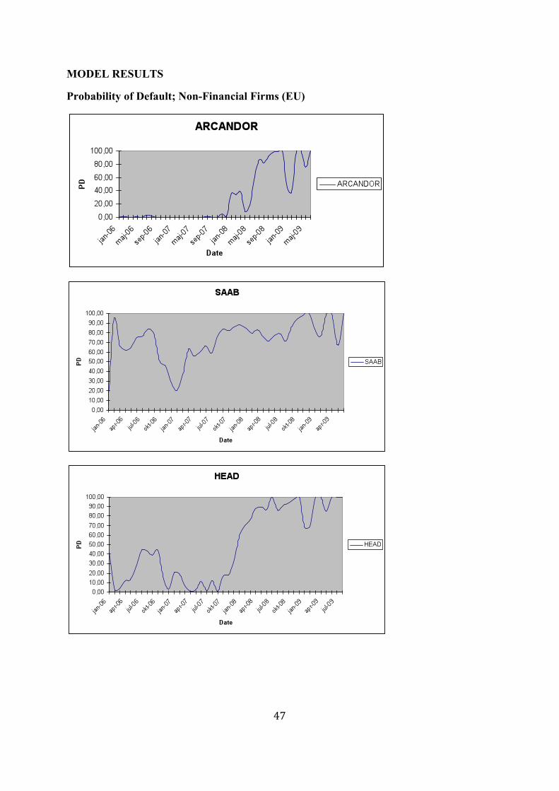
7.1.1 Defaulted Non-Financial Firms
The defaulted non-financial firms from the EU included in the study are Arcandor AG,
SAAB, Head NV and Magyar Telecom.

32
On September 16th 2008, the stock price of Arcandor fell twenty percent following an
announcement about the company’s poor financial health.67 Due to liquidity problems,
Arcandor requested financial assistance from the government in May 2009. In June, the
company declared that they were no longer able to fulfil their rent obligations and filed for
Chapter 11 in the 9th of June in 2009.68 Already 1,5 years before the event of default, a
tendency of default is visible in our results. The probability increases continuously until the
default date, showing extremely high values right after the fall of the stock price.
Ever since SAAB was bought by General Motors in 2000, the losses have been significantly
large. In February 2009, GM declares that they will no longer cover the losses and SAAB
soon applies for reconstruction of the company. On the 2nd of June the same year, the
company enters default.69 The high liquidity problems of the company are shown in the
probability rates already in the beginning of the period.
According to Standard & Poor’s, the liquidity of HEAD NV has been weak during a longer
time period. On August 14 2009, the company defaults.70 Our estimates give early predictions
of the default, showing high probabilities already in the beginning of 2008.
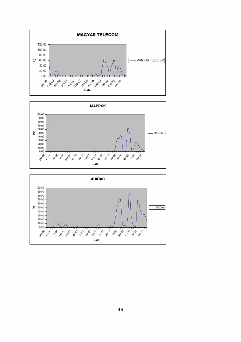
Weaker Hungarian exchange rates by the end of 2008 and decreasing stock prices in 2008-
2009 were some of the reasons which lead to a default of Magyar Telecom NV on the 4th of
November in 2009.71 We can observe relatively high default probabilities during this time,
being much lower the months before.
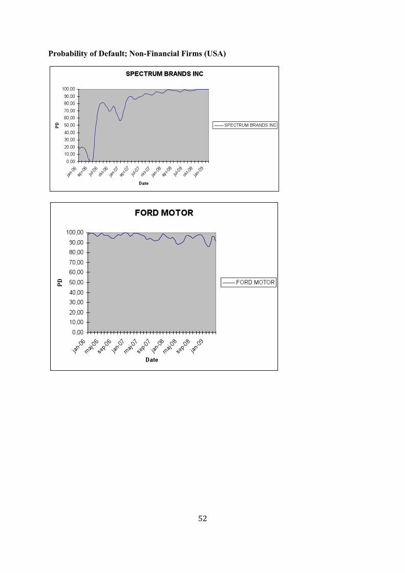
The defaulted American non-financial companies, included in our study, are Spectrum Brands
Inc, Ford Motor, The McClatchy Company and Spansion Inc.
Spectrum Brands Inc has been highly leveraged during the whole period. Because of the large
amount of debt, the company tried to sell off one of their divisions, without success. On the
67 Reuters (http://www.reuters.com/article/idUSLG65509220080916) 68 Arcandor AG (http://www.arcandor.de/en/presse/211.asp) 69 SAAB (http://www.saabgroup.com/) 70 Standard & Poor’s (http://www.standardandpoors.com) 71 Magyar Telecom BV (http://www.telekom.hu/main)
33
4th of February 2009, the company defaulted and further filed for Chapter 11.72 The high
leverage during the period is shown in the default probabilities, predicting default already
from the beginning of the period.
In December 2006, Ford Motor raised its borrowing capacity with a substantial amount of 25
billion dollars. In 2006 and 2007, the company reported large amounts of losses. In June
2008, Ford sold off its subsidiaries Jaguar and Land Rover. In November the same year, Ford,
GM and Chrysler together sought for governmental financial aid. On the 6th of April 2009,
the company defaulted.73 The probability values of Ford have been extremely high during the
entire time period.
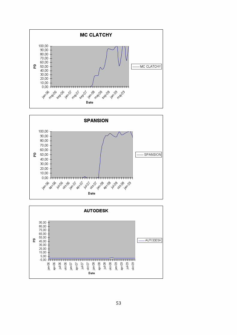
In March 2006, The McClatchy Company announced their plan to acquire Knight Ridder.
After this date, the stock value of McClatchy has decreased continuously, resulting in a value
lower than one dollar in December 2008. On the 29th of June in 2009, the company
defaulted.74 The default probabilities started to increase significantly 1,5 years prior the event
of default.
The share price of Spansion Inc began to fall in the beginning of 2007 and the company
defaulted on the 15th of January in 2009. On the 1st of March in 2009, Spansion Inc filed for
Chapter 11.75 The default probabilities of Spansion Inc started to rise about one year before
the default date.
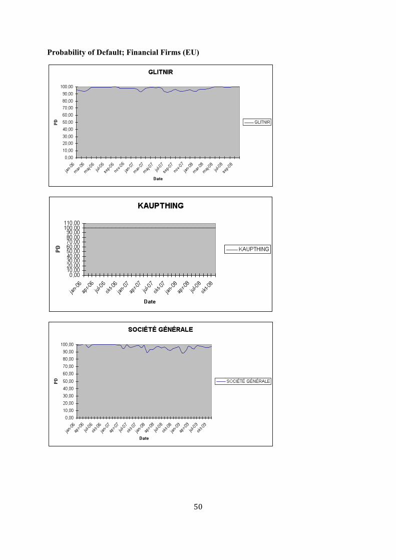
7.1.2 Defaulted Financial Firms
The defaulted financial firms from the EU which are included in the study are Glitnir and
Kaupthing, two Icelandic banks. Iceland has been especially affected by the financial crisis,
having three of the major banks defaulted. A severe inflation and a weak currency are the
results of the crisis.
72 Spectrum Brands Inc (http://www.spectrumbrands.com) 73 Ford Motor Corporation (http://www.ford.com) 74 The McClatchy Company (http://www.mcclatchy.com/) 75 Spansion Inc (http://www.spansion.com/Pages/default.aspx)
34
Glitnir was nationalized on the 7th of October in 2008 when the government of Iceland
acquired large parts of the bank. A few days later, Glitnir’s Norwegian subsidiary was sold
and on the 29th of October the same year, the bank defaulted. In February 2009, the bank
changed its name to Islandsbanki.76 Our estimates are high during the entire period of 2006-
2008, probably due to the severe crisis in Iceland.
Kaupthing Bank was defaulted and nationalized on the 9th of October 2008.77 The probability
values we receive from our model are extremely high during the time period, probably due to
the crisis in the country.
We have also included two defaulted American financial firms in the study; Bear Sterns and
Lehman Brothers. As mentioned in the introductory part, the worldwide financial crisis
started in the USA. The trigger was the American housing bubble and their connected
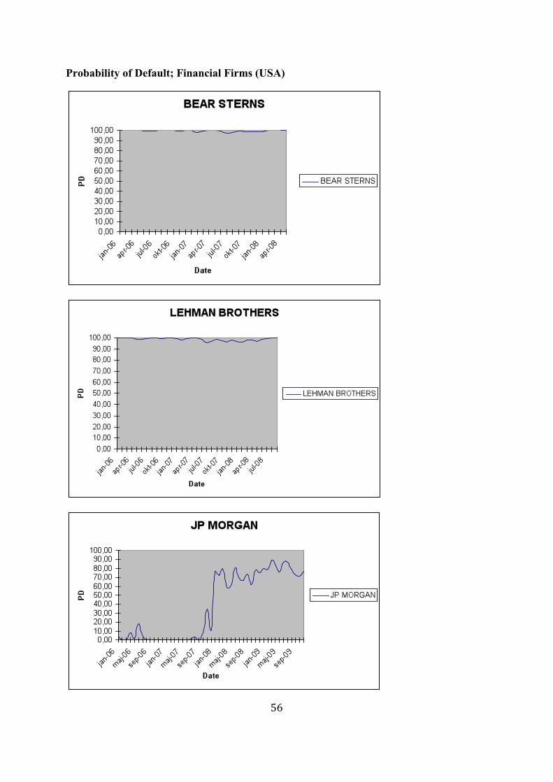
mortgage backed securities (2006-2007).
Bear Sterns was one of the banks deeply involves with the MBS-problems and was therefore
quickly affected by the crisis. In March 2008, the Federal bank of New York, offered an
emergency loan to the bank without success. At last, the bank was sold at fire sale78 to JP
Morgan in March 2008. On the 24th of May, the company defaulted.79 Due to the severe
problems, liquidity issues and high liabilities of the bank, the default probabilities are high
already in the beginning of 2006.
Until the beginning of 2008, Lehman Brothers declared good results. Although, Lehman
Brothers was just like Bear Sterns one of the main underwriters of the mortgage backed
securities which lead to a decline in the share price and a default on the 15th of September
2008.80 The probability values have been just as high as the ones of Bear Sterns even though
their problems occurred at a later time.
76 Islandsbanki (http://www.islandsbanki.is/english/) 77 Kaupthing Bank (http://www.kaupthing.com/?pageid=4131) 78 Defined as a situation in which the prices of the securities are considered to be very low. (Investopedia.com) 79 New York Times (http://www.nytimes.com/2008/03/17/business/17bear.html) 80 Bloomberg (http://www.bloomberg.com/apps/news?sid=awh5hRyXkvs4&pid=20601087)
35
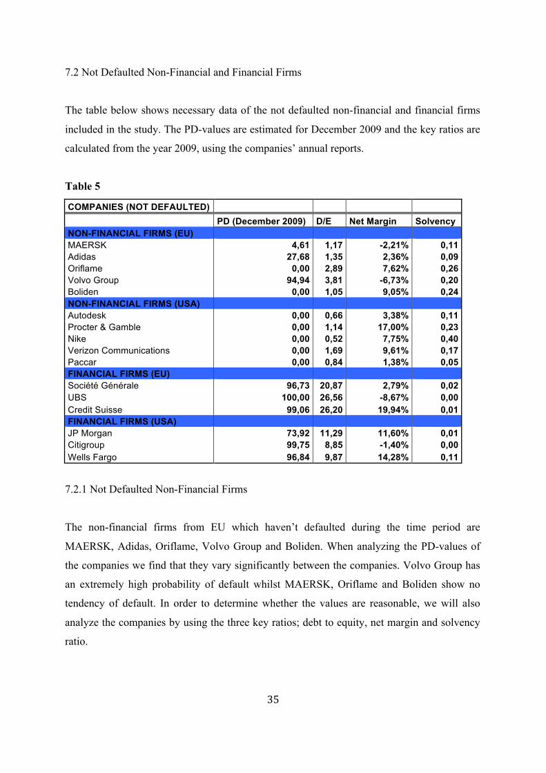
7.2 Not Defaulted Non-Financial and Financial Firms
The table below shows necessary data of the not defaulted non-financial and financial firms
included in the study. The PD-values are estimated for December 2009 and the key ratios are
calculated from the year 2009, using the companies’ annual reports.
Table 5
COMPANIES (NOT DEFAULTED) PD (December 2009) D/E Net Margin Solvency NON-FINANCIAL FIRMS (EU) MAERSK 4,61 1,17 -2,21% 0,11 Adidas 27,68 1,35 2,36% 0,09 Oriflame 0,00 2,89 7,62% 0,26 Volvo Group 94,94 3,81 -6,73% 0,20 Boliden 0,00 1,05 9,05% 0,24 NON-FINANCIAL FIRMS (USA) Autodesk 0,00 0,66 3,38% 0,11 Procter & Gamble 0,00 1,14 17,00% 0,23 Nike 0,00 0,52 7,75% 0,40 Verizon Communications 0,00 1,69 9,61% 0,17 Paccar 0,00 0,84 1,38% 0,05 FINANCIAL FIRMS (EU) Société Générale 96,73 20,87 2,79% 0,02 UBS 100,00 26,56 -8,67% 0,00 Credit Suisse 99,06 26,20 19,94% 0,01 FINANCIAL FIRMS (USA) JP Morgan 73,92 11,29 11,60% 0,01 Citigroup 99,75 8,85 -1,40% 0,00 Wells Fargo 96,84 9,87 14,28% 0,11
7.2.1 Not Defaulted Non-Financial Firms
The non-financial firms from EU which haven’t defaulted during the time period are
MAERSK, Adidas, Oriflame, Volvo Group and Boliden. When analyzing the PD-values of
the companies we find that they vary significantly between the companies. Volvo Group has
an extremely high probability of default whilst MAERSK, Oriflame and Boliden show no
tendency of default. In order to determine whether the values are reasonable, we will also
analyze the companies by using the three key ratios; debt to equity, net margin and solvency
ratio.
36
As mentioned, MAERSK has a low PD-value, indicating a low risk of default. The key ratios
show that the company has a larger share of debt than equity, negative profits and a solvency
which is lower than what is generally desired. The key ratios therefore imply that the PD-
value should be higher.81 Although, it should be mentioned that the industry is capital intense
and that the company has a strong cash flow relative its main competitors.82
Adidas receives a default probability of almost 30% at the end of 2009. The company has a
positive net margin but a relatively weak solvency. The amount of debt is 35% larger than the
shareholders’ equity. The amount of debt as well as a decreased stock price during the year
affects the PD value which can be considered relatively high.
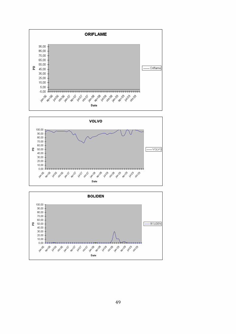
The PD value of Oriflame is zero by the end of 2009 as well as during the rest of the time
period. The key ratios also indicate that Oriflame is a strong company and we believe that a
reason for this is that this industry isn’t as cyclical as other industries and therefore has
managed relatively well during the crisis.
Volvo Group has an extremely high probability of default, with a value of almost 95%. As
mentioned earlier, the motor vehicle industry has been struck hard by the financial crisis. The
key ratios indicate problems within the company as well, having a large amount of liabilities
and a negative profit margin. The share price has decreased since the beginning of 2008 and
the operating cash flow has been weak during 2009.83
Boliden has a default probability equal to zero which can be supported by the values of the
key ratios. The company has a strong net margin as well as a high solvency ratio.
The American non-financial firms which haven’t defaulted are Autodesk, Procter & Gamble,
Nike, Verizon Communications and Paccar. In USA, the default probabilities are zero for all
of the included companies. The key ratios imply the same results since all companies’ debt to
equity ratios are relatively low except for Verizon Communications. The reason for their low
81 MAERSK (http://www.maersk.com/Pages/default.aspx) 82 Annual Reports (2009) of MAERSK (http://www.maersk.com/Pages/default.aspx) and its main competitors Mitsui OSK Lines Ltd (http://www.mol.co.jp/menu-e.html), Neptune Orient Lines Ltd (http://www.nol.com.sg/index.html), Nippon Yusen Kabushiki Line (http://www2.nykline.com/) 83 Volvo Group (http://www.volvo.com/group/volvosplash-global/en-gb/volvo_splash.htm)

37
probability value is probably their high net margin and solvency. It is interesting that Paccar
has managed this well during the crisis, considering the problems in the industry.
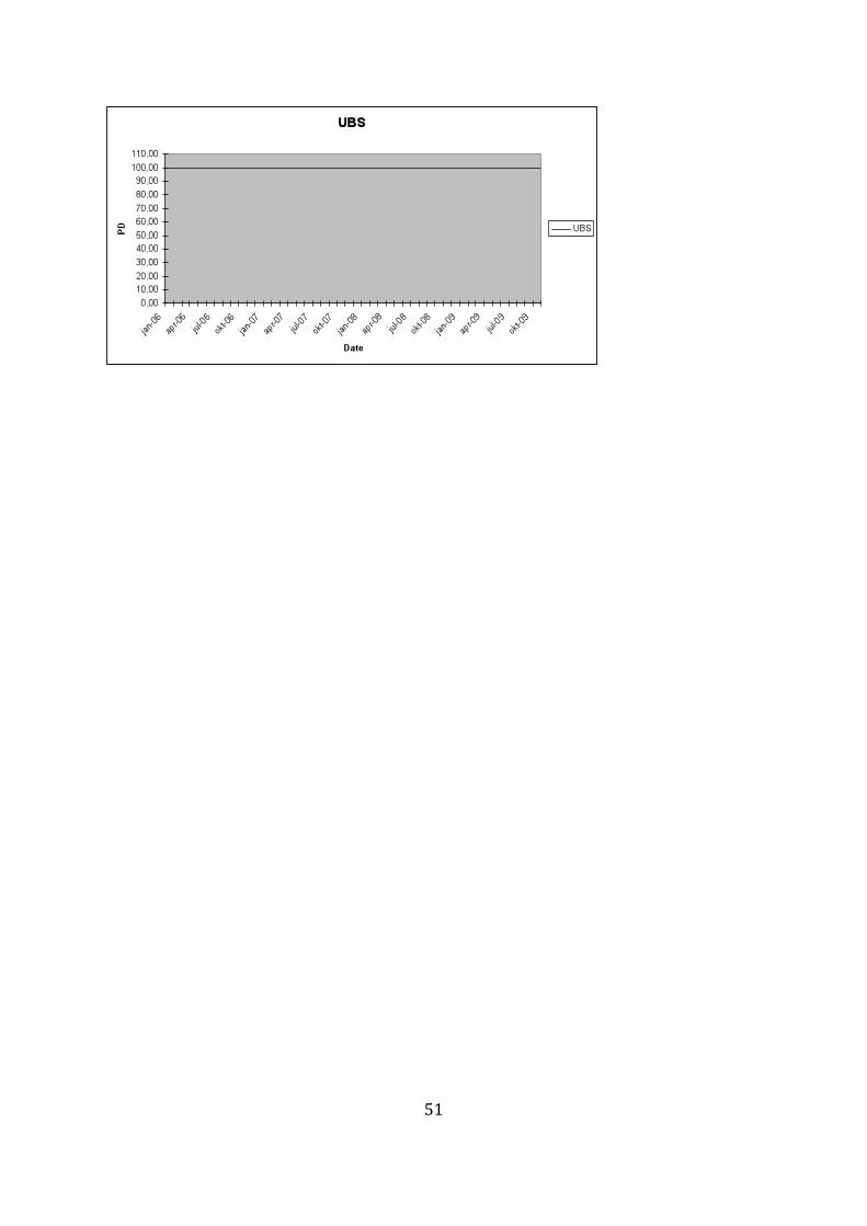
7.2.2 Not Defaulted Financial Firms
In the study, we have included the financial firms Société Générale, UBS and Credit Suisse
from the EU. The American financial firms included are JP Morgan, Citigroup and Wells
Fargo. Scott Talbott, senior vice president of government affairs at the Financial Services
Roundtable84, makes the following announcement in the New York Times; “Our analysis
shows that the banks have varying degrees of solvency and does not reveal that any
institution is insolvent”.85 Due to this announcement we have decided not to analyze this ratio
further. Our estimates show that all banks, both the ones from the EU and the USA, have
extremely high default probabilities during the entire time period. The financial crisis has
globally damaged financial institutions. Since the crisis started within this industry, it is
obvious that the default probabilities have been high as early as our predictions show. Among
the banks from the EU we see that the debt to equity ratios indicate the same conclusion as
the default probabilities do. All banks have default probabilities above 96%. Only JP Morgan
has a lower default probability than 96%, instead having a PD value of approximately 74%.
Their debt to equity ratio is significantly larger than the other banks but the net margin is
much higher. One of the reasons for the better result might be that their share value has
remained the same during the period 2006-2009 whilst the other banks’ share prices have
decreased significantly since 2008. We find that the banks from EU and USA have different
net margins. Although, this fact clearly doesn’t affect the values of the default probabilities.
7.3 Discussion of the Results
In this part, we will try to determine which of the economies, USA or EU, give the best
predictions based on the results above. As mentioned, we will separate financial and non-
financial companies.
84 A trade group whose members include the largest American banks. 85 New York Times (http://www.nytimes.com/2009/02/13/business/worldbusiness/13iht-13insolvent.20163493.html)
38
7.3.1 Non-Financial Firms
For the defaulted non-financial firms from the EU, we can determine that the model has been
able to capture the risk of default well, showing increased probabilities approximately 1,5
years before the default event. In the case of Saab, the PD-values have been relatively large
during the whole period, increasing from 60% to 80% approximately 1,5 years before the
default. Head shows a similar result, predicting 40% default probability before the strong
increase to 70% 1,5 years before the default. Magyar Telecom BV shows low default
probabilities during the whole period. Even though the values increased 1,5 years before the
default, the values were extremely low the months before the default event. Decreasing PD
values in relation with the default might depend on a merger with Cable TV subsidiaries T-
Kabel Hungary and Del-Vonal at that time.86
The predictions about the non-defaulted non-financial firms are not as easy to analyze. What
we find is that the default probabilities of both Adidas, Oriflame, Volvo Group and Boliden
seem reasonable when comparing to the “health” of the companies. The key ratios of
MAERSK on the other hand indicate a higher risk than the default probabilities show.
The model generates reliable PD-values for the American defaulted non-financial firms as
well. The high liabilities of Spectrum Brands and Ford Motor during the whole time period
are followed by high PD values from the beginning of the period. The PD values of
McClatchy started to increase 1,5 years before the default. In contrast, the default
probabilities of Spansion Inc didn’t increase until one year before the default of the company.
All of the companies which haven’t defaulted during the period generate default probabilities
equal to zero. Comparing these values to the “health” of the companies, we find that they
seem reasonable. Autodesk, Procter & Gamble, Nike, Verizon Communications and Paccar
all show proof of strengths within the companies.
All in all, the model has been able to predict the probability of default in EU approximately
1,5 years before the event of default. Drawbacks can be seen in the case of Magyar where low
PD-values are observed despite the default of the company (Type I-error). The model has also
86 Magyar Telecom BV (http://www.telekom.hu/about_magyar_telekom/company_history)
39
generated reasonable default probabilities in the USA where the values seem to match with
the companies and their financial history.
7.3.2 Financial Firms
Since the default probabilities of all of our chosen financial firms are extremely high, it is
difficult to make a comparative analysis between the economies. The financial crisis has had
a great impact on this industry which has lead to high risks and large problems within the
companies. Since financial institutions generally have high debt to equity ratios, especially
during a financial crisis, they will generate high default probabilities. Large amounts of
liabilities aren’t always reason enough for default. If a company has good margins and a
strong cash flow, they have good opportunities to handle the risks from the debt. An example
of this from our study is Credit Suisse which has a strong net margin of approximately 20%
(Type II-error). Note that we only use two key ratios in the analysis and that there are other
parameters affecting the risks of the company as well.
When calculating the probability of default of the financial firms, we used the capital
requirement of Basel I, 8%, in the DC formula. If the capital requirement instead would have
been based on the firm’s rating (Basel II), the estimates probably would have been different.
By using Basel II, it would be possible to capture the companies’ health in a better way when
predicting the default probabilities.
40
8. CONCLUSION
8.1 Final Discussion
It is difficult to draw any conclusions about the difference in default predictions between the
non-financial firms from the EU and the USA since the study is qualitative and only includes
a minor number of companies. Although, our results indicate that there are no significantly
large differences in the predictions. Our study also shows that the model predicts a default on
average 1,5 years before the default actually occurs.
Since the financial crisis has affected financial companies especially bad, leading to a severe
increase in their already high leverage, the default probabilities of these companies are
extremely high. The high probability values as well as the similarities between the companies
make it difficult for us to draw any conclusions about this industry.
It should be mentioned that a financial firm is protected by its government to a larger extent
than non-financial firms. This affects the actual default probability of these companies but
will not be shown in the model. Our results show higher default probabilities during a longer
time among financial firms than non-financial firms. This might depend on the fact that the
crisis has its origin within this industry.
From our study we can conclude that a high default probability generally is connected with an
actual default of the company. Although, there are deviations from this conclusion. In our
study, we have an example of this where the default probability is high but the company
seems reasonably healthy. The reason for this might be the high volatility in the market due to
the current financial crisis. We further came across the opposite problem where a defaulted
company generated low default probabilities. The reason for this problem can for example be
an unexpected set-back of the company.
Earlier in the thesis we show that Moody’s KMV model has been able to make better
predictions than for example Standard & Poor’s. The results of our study are in line with this

41
conclusion, showing that the model generates accurate predictions, which further indicate that
the KMV model is an advantage of Moody’s relative other agencies.
8.2 Further Research
Since our study is qualitative, including a minor number of companies, the results are only an
indication of the differences in the predictions of default probabilities. An idea would be to
perform a study including a larger number of companies in order to find more significant
results. Further, since several defaulted companies generated extremely high default
probabilities during the whole time period, it would be interesting to analyze a longer time
period. This would make it possible to find out how long time ahead the actual default the
model was able to predict the event. Since the default probabilities of financial firms turned
out to be relatively poor estimates, it would be interesting to examine how the capital
requirements of Basel II would affect the probabilities.
42
9. REFERENCES
Arcandor AG, Homepage: http://www.arcandor.de/en/presse/211.asp, retrieved 25-05-2009 Bank of International Settlements (BIS), Homepage: http://www.bis.org/about/index.htm, retrieved 03-05-2010 http://bis.org/bcbs/index.htm#Consultative_Group, retrieved 03-05-2010 http://www.bis.org/publ/bcbs04b.pdf?noframes=1, retrieved 03-05-2010 http://www.bis.org/publ/g10.htm, retrieved 03-05-2010 http://www.bis.org/publ/bcbs_nl11.htm, retrieved 03-05-2010 http://www.bis.org/publ/bcbsca01.pdf, retrieved 02-05-2010 Bharath, S.T. & Shumway, T. (2004) Forecasting Default with the KMV-Merton Model, Working Paper, The University of Michigan Bloomberg, Homepage:
http://www.bloomberg.com/apps/news?sid=awh5hRyXkvs4&pid=20601087, retrieved 25-05-2009
Chan-Lau, J. A. & Sy, A. N. R. (Sep 2006) Distance-to-Default in Banking: A Bridge Too Far?, IMF Working Paper, WP/06/215 Crosbie, P.J. & Bohn, J.R. (2003) Modeling Default Risk: Modeling Methodology. Moody’s KMVTM working paper Dagens Industri, Homepage: http://www.di.se/trader, retrieved 03-05-2010
http://www.e24.se/business/bank-och-finans/hang-med-i-finanskrisens-alla-svangar_777413.e24, retrieved 02-05-2010
Delianedis, G. & Geske, R. (1998) Credit risk and risk neutral default probabilities: Information about rating migrations and defaults, Finance, Anderson Graduate school of Management, UC Los Angeles Dwyer, D. W. (2006) The Distribution of Defaults and Bayesian Model Validation, Research Paper, Moody's KMV European Central Bank (ECB), Homepage: http://www.ecb.int/press/key/date/2005/html/sp050415.en.html, retrieved 14-05-2010
http://www.ecb.int/stats/html/index.en.html, Statistics Pocket Book 2009, retrieved 14-05-2010
http://www.ecb.int/ecb/history/emu/html/index.en.html#stage2, retrieved 28-05-2010
43
European Commission (EC), Homepage: http://ec.europa.eu/external_relations/us/index_en.htm, retrieved 14-05-2010
http://ec.europa.eu/enterprise/policies/international/cooperating-governments/usa/transatlantic-economic-council/index_en.htm#h2-areas-of-cooperation, retrieved 14-05-2010
http://ec.europa.eu/external_relations/us/economic_en.htm, retrieved 14-05-2010 http://ec.europa.eu/trade/creating-opportunities/bilateral-relations/countries/united-states/index_en.htm, 14-05-2010 http://trade.ec.europa.eu/doclib/docs/2006/september/tradoc_113465.pdf, retrieved 28-05-2010
Ford Motor Company, Homepage: http://www.ford.com, retrieved 25-05-2009 Gapen, M. (2009) Measuring and Forecasting Financial Stability, workshop by Deutsche Bundesbank and Technische Universtät Dresden HQ Bank, Homepage:
http://www.hq.se/sv/Strukturerade-produkter/Marknadsinformation/hq-kurslista/USA-vs-Europa/, retrieved 02-05-2010
Investopedia: http://www.investopedia.com Islandsbanki, Homepage: http://www.islandsbanki.is/english/, retrieved 25-05-2009 Kaupthing Bank, Homepage: http://www.kaupthing.com/?pageid=4131, retrieved 25-05-2009 Kealhofer, S. & Kurbat, M. (2000) Benchmarking Quantitative Default Risk Models: A Val-idation Methodology, Research Paper, Moody's KMV Keidel, A. (2008) The Global Financial Crisis: Lessons for the United States and China, Based on a luncheon speech delivered for the U.S.-China Business Council at the Fairmont Hotel in Washington, D.C. Korablev, I. & Dwyer, D. W. (2007) Power and Level Validation of Moody’s KMV EDF™ Credit Measures in North America, Europe and Asia, Research Paper, Moody's KMV Korablev, I. & Qu, S. (2009) Validating the Public EDF™ Model Performance during the Credit Crisis, Research Paper, Moody's KMV MAERSK, Homepage: http://www.maersk.com/Pages/default.aspx, retrieved 26-05-2009 Magyar Telecom BV, Homepage: http://www.telekom.hu/main, retrieved 25-05-2009 http://www.telekom.hu/about_magyar_telekom/company_history, retrieved 27-05-2010

44
Merton R. C., (1973) On the Pricing of Corporate Debt: The Risk Structure of Interest Rates*, presented at the American Finance Association Meeting, New York Mitsui OSK Lines Ltd, Homepage: http://www.mol.co.jp/menu-e.html, retrieved 27-05-2010 Moody’s, Homepage: http://www.moodyskmv.com/cpc06/pres/01_Deloitte.pdf, retrieved 02-05-2010 http://www.moodyskmv.com/research/files/Enron.pdf, retrieved 27-05-2010 Neptune Orient Lines Ltd, Homepage: http://www.nol.com.sg/index.html, retrieved 27-05-2010 Nippon Yusen Kabushiki Line, Homepage: http://www2.nykline.com/, retrieved 27-05-2010 Ogden, J. P., Jen, F. C. & O’Connor, P. F. (2002) Advanced Corporate Finance: Policies and Strategies, Prentice Hall, New Jersey Reuters, Homepage: http://www.reuters.com/article/idUSLG65509220080916, retrieved 25-05-2009 SAAB, Homepage: http://www.saabgroup.com/, retrieved 25-05-2009 Saunders, A. & Allen L. (2002) Credit Risk Measurement; New Approaches to Value at Risk and Other Paradigms, Second Edition, John Wiley & Sons, Inc., New York Sobehart, J., Keenan, S. & Stein, R. (2001) Benchmarking Quantitative Default Risk Models, A Validation Methodology, Algo Research Quarterly, Vol. 4, NOS. ½, March/June Sobehart, J., Keenan, S. & Stein, R. (2000), Rating Methodology, Benchmarking Quantitative Default Risk Models, A Validation Methodology, Research paper, Moody’s Investors Service Spanion Inc., Homepage: http://www.spansion.com/Pages/default.aspx, retrieved 25-05-2009 Spectrum Brands Inc., Homepage: http://www.spectrumbrands.com, retrieved 25-05-2009 Standard & Poor’s, Homepage: http://www.standardandpoors.com, retrieved 25-05-2009 The McClatchy Company, Homepage: http://www.mcclatchy.com/, retrieved 25-05-2009

45
The New York Times, Homepage: http://www.nytimes.com/2008/03/17/business/17bear.html, retrieved 25-05-2009
http://www.nytimes.com/2009/02/13/business/worldbusiness/13iht-13insolvent.20163493.html, retrieved 26-05-2009
Volvo Group, Homepage:
http://www.volvo.com/group/volvosplash-global/en-gb/volvo_splash.htm, retrieved 26-05-2009
Worldbank, Homepage: http://rru.worldbank.org/documents/CrisisResponse/Note8.pdf, retrieved 28-05-2010
46
APPENDIX
Figure 1
CASE STUDY ENRON; COMPARISON BETWEEN S&P AND MOODY’S – PROBABILITY OF DEFAULT
47
MODEL RESULTS
Probability of Default; Non-Financial Firms (EU)
48
49
50
Probability of Default; Financial Firms (EU)
51
52
Probability of Default; Non-Financial Firms (USA)
53

54

55
56
Probability of Default; Financial Firms (USA)
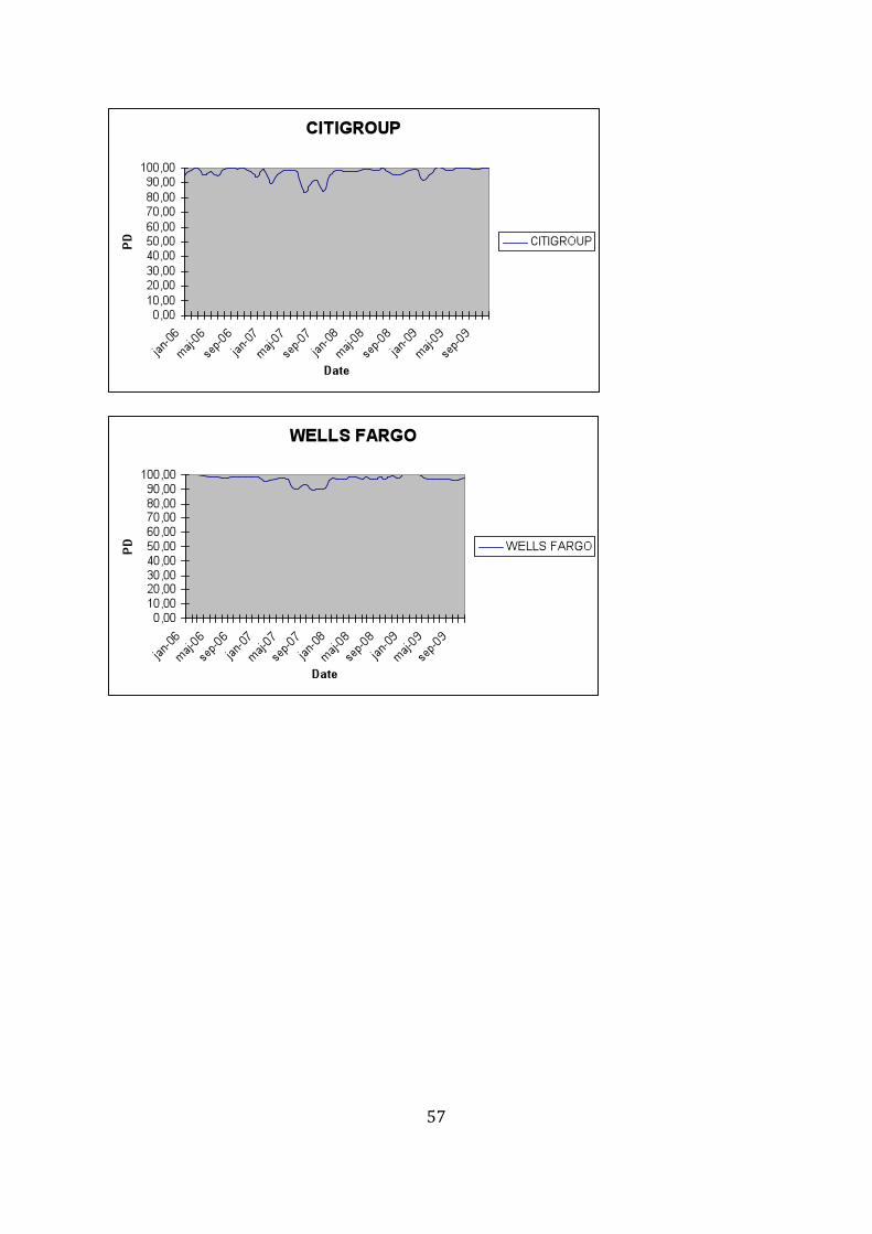
57