Predicting success of government

intervention during GFC

Pearpilai Jutasompakorn

2013

Disclaimer and Copyright

The material in this report is copyright of Pearpilai Jutasompakorn. The views and opinions expressed in this report are solely that of the author’s and do not reflect the views and opinions of the Australian Prudential Regulation Authority. Any errors in this report are the responsibility of the author. The material in this report is copyright. Other than for any use permitted under the Copyright Act 1968, all other rights are reserved and permission should be sought through the author prior to any reproduction.

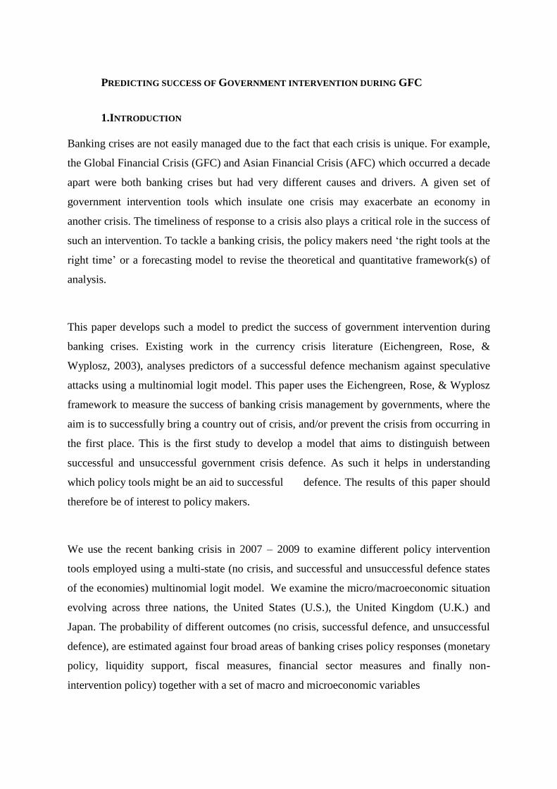
PREDICTING SUCCESS OF GOVERNMENT INTERVENTION DURING GFC

1.INTRODUCTION

Banking crises are not easily managed due to the fact that each crisis is unique. For example,

the Global Financial Crisis (GFC) and Asian Financial Crisis (AFC) which occurred a decade

apart were both banking crises but had very different causes and drivers. A given set of

government intervention tools which insulate one crisis may exacerbate an economy in

another crisis. The timeliness of response to a crisis also plays a critical role in the success of

such an intervention. To tackle a banking crisis, the policy makers need ‘the right tools at the

right time’ or a forecasting model to revise the theoretical and quantitative framework(s) of

analysis.

This paper develops such a model to predict the success of government intervention during

banking crises. Existing work in the currency crisis literature (Eichengreen, Rose, &

Wyplosz, 2003), analyses predictors of a successful defence mechanism against speculative

attacks using a multinomial logit model. This paper uses the Eichengreen, Rose, & Wyplosz

framework to measure the success of banking crisis management by governments, where the

aim is to successfully bring a country out of crisis, and/or prevent the crisis from occurring in

the first place. This is the first study to develop a model that aims to distinguish between

successful and unsuccessful government crisis defence. As such it helps in understanding

which policy tools might be an aid to successful defence. The results of this paper should

therefore be of interest to policy makers.

We use the recent banking crisis in 2007 – 2009 to examine different policy intervention

tools employed using a multi-state (no crisis, and successful and unsuccessful defence states

of the economies) multinomial logit model. We examine the micro/macroeconomic situation

evolving across three nations, the United States (U.S.), the United Kingdom (U.K.) and

Japan. The probability of different outcomes (no crisis, successful defence, and unsuccessful

defence), are estimated against four broad areas of banking crises policy responses (monetary

policy, liquidity support, fiscal measures, financial sector measures and finally non-

intervention policy) together with a set of macro and microeconomic variables

2

2. THE MODEL

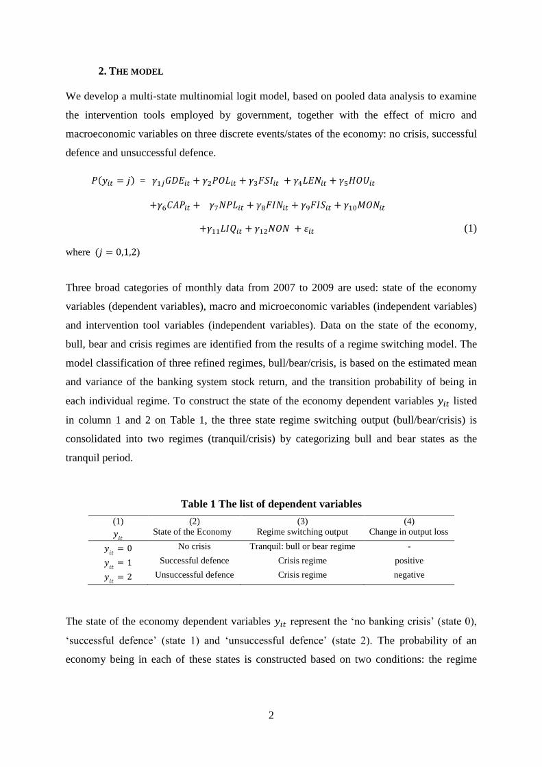
We develop a multi-state multinomial logit model, based on pooled data analysis to examine

the intervention tools employed by government, together with the effect of micro and

macroeconomic variables on three discrete events/states of the economy: no crisis, successful

defence and unsuccessful defence.

( ) =

(1)

where ( )

Three broad categories of monthly data from 2007 to 2009 are used: state of the economy

variables (dependent variables), macro and microeconomic variables (independent variables)

and intervention tool variables (independent variables). Data on the state of the economy,

bull, bear and crisis regimes are identified from the results of a regime switching model. The

model classification of three refined regimes, bull/bear/crisis, is based on the estimated mean

and variance of the banking system stock return, and the transition probability of being in

each individual regime. To construct the state of the economy dependent variables listed

in column 1 and 2 on Table 1, the three state regime switching output (bull/bear/crisis) is

consolidated into two regimes (tranquil/crisis) by categorizing bull and bear states as the

tranquil period.

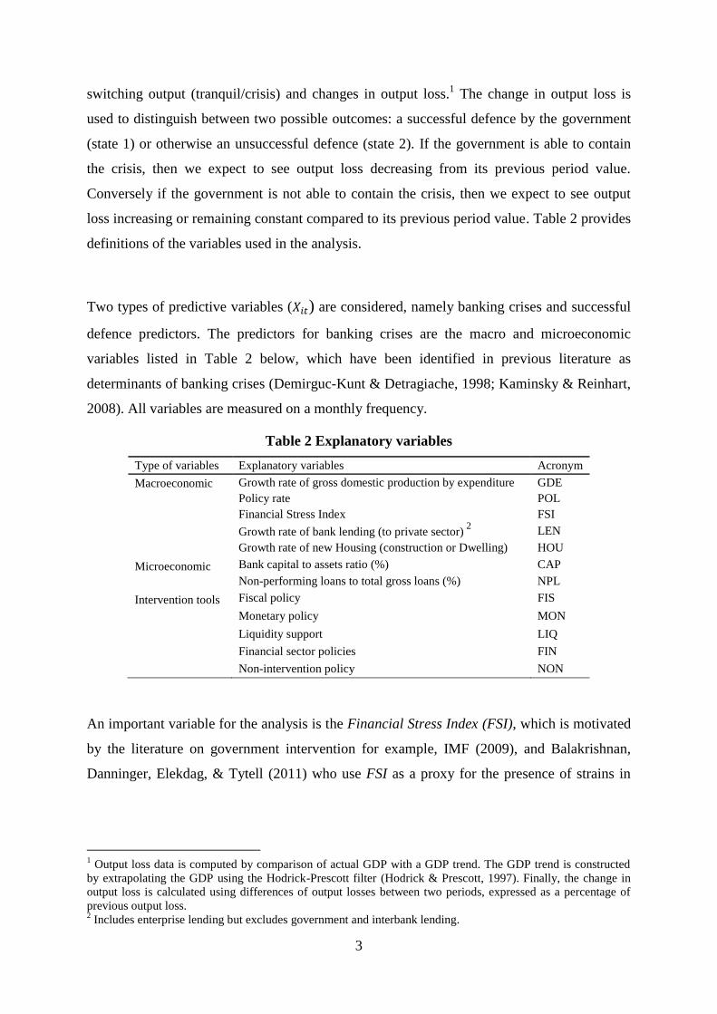
Table 1 The list of dependent variables

(1)

(2)

State of the Economy

(3)

Regime switching output

(4)

Change in output loss

No crisis Tranquil: bull or bear regime -

Successful defence Crisis regime positive

Unsuccessful defence Crisis regime negative

The state of the economy dependent variables represent the ‘no banking crisis’ (state 0),

‘successful defence’ (state 1) and ‘unsuccessful defence’ (state 2). The probability of an

economy being in each of these states is constructed based on two conditions: the regime

3

switching output (tranquil/crisis) and changes in output loss.1 The change in output loss is

used to distinguish between two possible outcomes: a successful defence by the government

(state 1) or otherwise an unsuccessful defence (state 2). If the government is able to contain

the crisis, then we expect to see output loss decreasing from its previous period value.

Conversely if the government is not able to contain the crisis, then we expect to see output

loss increasing or remaining constant compared to its previous period value. Table 2 provides

definitions of the variables used in the analysis.

Two types of predictive variables ( ) are considered, namely banking crises and successful

defence predictors. The predictors for banking crises are the macro and microeconomic

variables listed in Table 2 below, which have been identified in previous literature as

determinants of banking crises (Demirguc-Kunt & Detragiache, 1998; Kaminsky & Reinhart,

2008). All variables are measured on a monthly frequency.

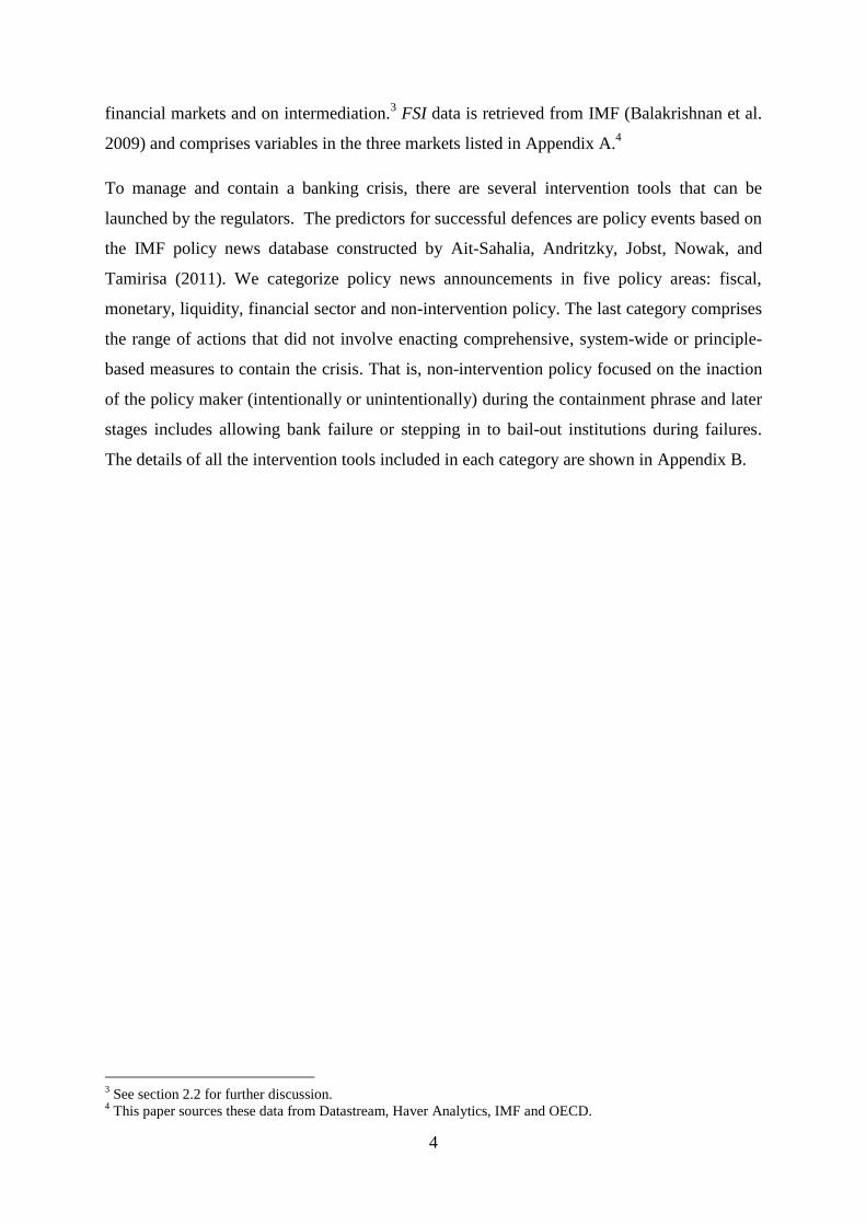
Table 2 Explanatory variables

Type of variables Explanatory variables Acronym

Macroeconomic Growth rate of gross domestic production by expenditure GDE

Policy rate POL

Financial Stress Index FSI

Growth rate of bank lending (to private sector)

2 LEN

Growth rate of new Housing (construction or Dwelling) HOU

Microeconomic Bank capital to assets ratio (%) CAP

Non-performing loans to total gross loans (%) NPL

Intervention tools Fiscal policy FIS

Monetary policy MON

Liquidity support LIQ

Financial sector policies FIN

Non-intervention policy NON

An important variable for the analysis is the Financial Stress Index (FSI), which is motivated

by the literature on government intervention for example, IMF (2009), and Balakrishnan,

Danninger, Elekdag, & Tytell (2011) who use FSI as a proxy for the presence of strains in

1 Output loss data is computed by comparison of actual GDP with a GDP trend. The GDP trend is constructed

by extrapolating the GDP using the Hodrick-Prescott filter (Hodrick & Prescott, 1997). Finally, the change in

output loss is calculated using differences of output losses between two periods, expressed as a percentage of

previous output loss. 2 Includes enterprise lending but excludes government and interbank lending.

4

financial markets and on intermediation.3 FSI data is retrieved from IMF (Balakrishnan et al.

2009) and comprises variables in the three markets listed in Appendix A.4

To manage and contain a banking crisis, there are several intervention tools that can be

launched by the regulators. The predictors for successful defences are policy events based on

the IMF policy news database constructed by Ait-Sahalia, Andritzky, Jobst, Nowak, and

Tamirisa (2011). We categorize policy news announcements in five policy areas: fiscal,

monetary, liquidity, financial sector and non-intervention policy. The last category comprises

the range of actions that did not involve enacting comprehensive, system-wide or principle-

based measures to contain the crisis. That is, non-intervention policy focused on the inaction

of the policy maker (intentionally or unintentionally) during the containment phrase and later

stages includes allowing bank failure or stepping in to bail-out institutions during failures.

The details of all the intervention tools included in each category are shown in Appendix B.

3 See section 2.2 for further discussion.

4 This paper sources these data from Datastream, Haver Analytics, IMF and OECD.

5

3. RESULTS

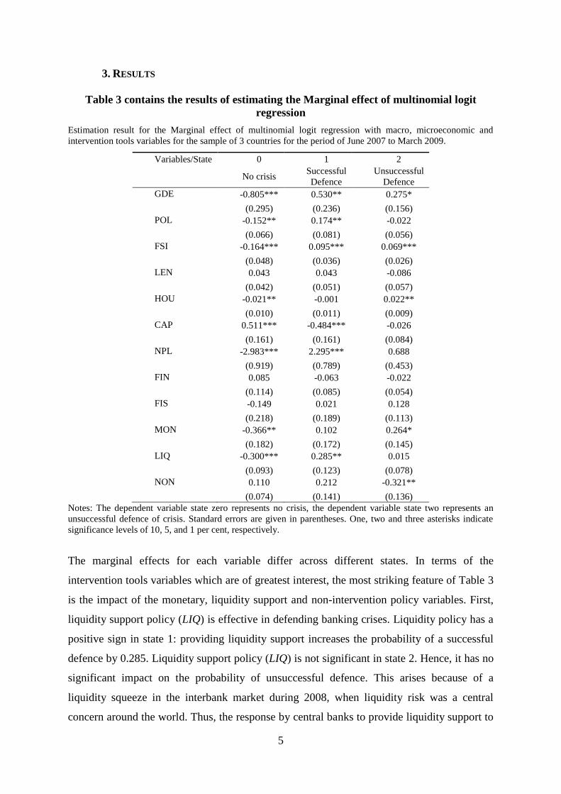
Table 3 contains the results of estimating the Marginal effect of multinomial logit

regression

Estimation result for the Marginal effect of multinomial logit regression with macro, microeconomic and

intervention tools variables for the sample of 3 countries for the period of June 2007 to March 2009.

Variables/State 0 1 2

No crisis Successful

Defence

Unsuccessful

Defence

GDE -0.805*** 0.530** 0.275*

(0.295) (0.236) (0.156)

POL -0.152** 0.174** -0.022

(0.066) (0.081) (0.056)

FSI -0.164*** 0.095*** 0.069***

(0.048) (0.036) (0.026)

LEN 0.043 0.043 -0.086

(0.042) (0.051) (0.057)

HOU -0.021** -0.001 0.022**

(0.010) (0.011) (0.009)

CAP 0.511*** -0.484*** -0.026

(0.161) (0.161) (0.084)

NPL -2.983*** 2.295*** 0.688

(0.919) (0.789) (0.453)

FIN 0.085 -0.063 -0.022

(0.114) (0.085) (0.054)

FIS -0.149 0.021 0.128

(0.218) (0.189) (0.113)

MON -0.366** 0.102 0.264*

(0.182) (0.172) (0.145)

LIQ -0.300*** 0.285** 0.015

(0.093) (0.123) (0.078)

NON 0.110 0.212 -0.321**

(0.074) (0.141) (0.136)

Notes: The dependent variable state zero represents no crisis, the dependent variable state two represents an

unsuccessful defence of crisis. Standard errors are given in parentheses. One, two and three asterisks indicate

significance levels of 10, 5, and 1 per cent, respectively.

The marginal effects for each variable differ across different states. In terms of the

intervention tools variables which are of greatest interest, the most striking feature of Table 3

is the impact of the monetary, liquidity support and non-intervention policy variables. First,

liquidity support policy (LIQ) is effective in defending banking crises. Liquidity policy has a

positive sign in state 1: providing liquidity support increases the probability of a successful

defence by 0.285. Liquidity support policy (LIQ) is not significant in state 2. Hence, it has no

significant impact on the probability of unsuccessful defence. This arises because of a

liquidity squeeze in the interbank market during 2008, when liquidity risk was a central

concern around the world. Thus, the response by central banks to provide liquidity support to

6

the financial system is crucial, as providing liquidity may be effective in supporting credit

supply to the private sector and alleviating the banking crisis duration. In addition, this

finding validates the importance of provision of liquidity support during a banking crisis as

found by many recent studies. Among others, Aït-Sahalia et al. (2011) suggest that liquidity

provision (in not only the U.S., but also in the U.K. and Japan) did help lower interbank risk

premiums and stabilize financial markets during this crisis. Likewise, Laeven and Valencia

(2010) confirm that initially, liquidity support and blanket guarantees were effective during

the containment phase.

While the results show liquidity support policy (LIQ) as a successful defence during the

crisis, the policy makers need to be certain that they are in crisis before using this tool.

Liquidity support policy (LIQ) has a negative sign in state 0: it decreases the probability of

having no crisis by approximately 0.3. This policy is perceived as a negative signal (that the

economy is in a worse stage than previously thought) thus increasing the public’s concern

about the soundness of the overall financial system. In short, liquidity support policy (LIQ)

can be a powerful tool if it is used at the right time, crisis period. On the other hand, if the

policy makers use the right tool at the wrong time, non-crisis period, it can exacerbate or drag

an economy into the crisis.

Government can decide to intervene, they can decide not to intervene or they can make no

decision and consequently do nothing. Non-intervention policy (NON) has a negative sign in

state 2: non-intervention and the decision to allow bank failures/bailouts decrease the

probability of an unsuccessful defence by 0.32. On the other hand, Non-intervention policy

(NON) is insignificant in states 0 and 1, suggesting a government deciding not to intervene,

has no effect on the probability of an economy not being in crisis but also has no effect on the

probability of a successful defence. Therefore, it seems that a government doing nothing or

making a conscious decision not to intervene does not harm in either crisis situation or in

normal time.

Though bank failures and bailouts may seem to be at different ends of the spectrum, these

policies reflect actions outside orderly resolution regimes or financial sector support

packages. Possibly, one of various approaches to policy making depends on a good

7

judgement to bail out viable banks and let non-viable banks fail. Bank bailouts consist of

approximately half of the interventions employed in Non-intervention policy (NON)

category, and are aimed at rescuing distressed financial intermediaries (FIs) to avoid the

immediate system turbulence and melt down.5 Bank bail-outs may lessen or avoid the risk of

contagion to other FIs or the systemic effect which might subsequently exacerbate the crisis.

Examples of ad hoc interventions to bail out troubled FIs during the subprime crisis include

the bailout of Bear Stearns in the United States, and guarantees to Northern Rock in the

United Kingdom (Brunnermeier, 2009; Laeven & Valencia, 2012, respectively).

Two plausible outcomes of making the wrong policy intervention can be compared from the

main findings. One possibility is when there is no crisis but policy makers misread the signs

and decide to intervene, for example with liquidity support policy (LIQ). This action can lead

to adverse outcome of decreasing the probability of an economy being in the non-crisis state.

Another possibility is that in a crisis the policy makers decide not to intervene or fail to

intervene (NON), but the approach leads to a decrease in the probability of unsuccessful

defence. These findings suggest that if the state of an economy is uncertain, intervention

should be procrastinated.

Monetary policy appears to be ineffective in defending against banking crises. As shown in

Table 3, monetary policy actions have a (marginally statistically significant) positive sign in

state 2. This intervention increases the probability of unsuccessful defence by 0.26, providing

some support for the conclusion that monetary policy is ineffective in mitigating strains in the

economy. One possible explanation is monetary policy operates with a lower bound on

interest rates in a weakened banking system. Consequently authorities have few options but

to mainly rely on quantitative and credit easing which is subject to debate in terms of its

effectiveness for the recent crisis and the past crisis in Japan in the 90s (Sellon, 2003).

Additionally, the public and banks may have interpreted monetary policy announcement

(MON) as evidence of forthcoming bad news about the soundness of other FIs even when the

economy is not in crisis. As shown in Table 3, monetary policy (MON) has a negative sign in

state 0: it decrease the probability of having no crisis by approximately 0.36. This associative

5 Non-intervention policy and bank failures/bailouts consist of 50 per cent of bank bailouts, 40 per cent of the

constant interest rate actions and 10 per cent of bank failures. We do not consider long term effects and market

discipline or the moral hazard argument in this study.

8

signalling leads to the observed relation rather than suggesting a causal relationship between

effectiveness of these tools and the state of the economy.

4. CONCLUSION

The results lead to the conclusion that the right tool tailored to the symptoms of a particular

crisis is needed to manage a banking crisis. Our findings suggest that during the GFC,

liquidity support policy (LIQ) is an effective intervention tool, rather than conventional

policies, such as fiscal and monetary policy, aimed at the economy more generally with

lagged effects. It was the right tool targeting the credit crunch facing the financial sector at

that time. Our conjecture is that the policy makers need to implement ‘the right tool(s) at the

right time’. The policy maker may consider employing a Non-intervention policy (NON)

when the stage of an economy is unknown.

The implication of our analysis for future government intervention is to carefully consider

timing and the tools for implementation after diagnosing the problem and state of economy.

Our main contribution has also been to link the findings of Diamon & Rajan (2005) that

banking system liquidity was an important determinant of the recent GFC, with the result that

liquidity also plays an important role in crisis prevention and management. In addition the

paper explores the effectiveness of other methods of government intervention in the 2007-

2009 credit and liquidity crunch.

9

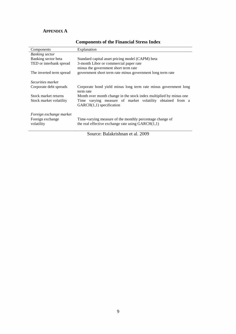
APPENDIX A

Components of the Financial Stress Index

Components Explanation

Banking sector

Banking sector beta Standard capital asset pricing model (CAPM) beta

TED or interbank spread

3-month Libor or commercial paper rate

minus the government short term rate

The inverted term spread government short term rate minus government long term rate

Securities market

Corporate debt spreads Corporate bond yield minus long term rate minus government long

term rate

Stock market returns Month over month change in the stock index multiplied by minus one

Stock market volatility Time varying measure of market volatility obtained from a

GARCH(1,1) specification

Foreign exchange market

Foreign exchange

volatility

Time-varying measure of the monthly percentage change of

the real effective exchange rate using GARCH(1,1)

Source: Balakrishnan et al. 2009

10

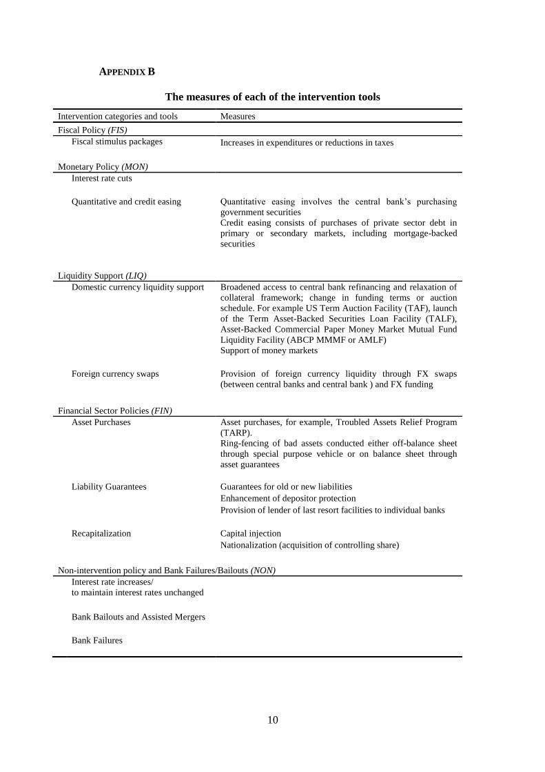
APPENDIX B

The measures of each of the intervention tools

Intervention categories and tools Measures

Fiscal Policy (FIS)

Fiscal stimulus packages Increases in expenditures or reductions in taxes

Monetary Policy (MON)

Interest rate cuts

Quantitative and credit easing Quantitative easing involves the central bank’s purchasing

government securities

Credit easing consists of purchases of private sector debt in

primary or secondary markets, including mortgage-backed

securities

Liquidity Support (LIQ)

Domestic currency liquidity support Broadened access to central bank refinancing and relaxation of

collateral framework; change in funding terms or auction

schedule. For example US Term Auction Facility (TAF), launch

of the Term Asset-Backed Securities Loan Facility (TALF),

Asset-Backed Commercial Paper Money Market Mutual Fund

Liquidity Facility (ABCP MMMF or AMLF)

Support of money markets

Foreign currency swaps Provision of foreign currency liquidity through FX swaps

(between central banks and central bank ) and FX funding

Financial Sector Policies (FIN)

Asset Purchases Asset purchases, for example, Troubled Assets Relief Program

(TARP).

Ring-fencing of bad assets conducted either off-balance sheet

through special purpose vehicle or on balance sheet through

asset guarantees

Liability Guarantees Guarantees for old or new liabilities

Enhancement of depositor protection

Provision of lender of last resort facilities to individual banks

Recapitalization Capital injection

Nationalization (acquisition of controlling share)

Non-intervention policy and Bank Failures/Bailouts (NON)

Interest rate increases/

to maintain interest rates unchanged

Bank Bailouts and Assisted Mergers

Bank Failures

11

REFERENCES

Ait-Sahalia, Y., Andritzky, J., Jobst, A., Nowak, S., & Tamirisa, N. (2011). Market response

to policy initiatives during the global financial crisis. Journal of International

Economics, 87(1), 162-177.

Balakrishnan, R., Danninger, S., Elekdag, S., & Tytell, I. (2011). The Transmission of

Financial Stress from Advanced to Emerging Economies. Emerging Markets Finance

& Trade, 47, 40-68.

Brunnermeier, M. K. (2009). Deciphering the liquidity and credit crunch 2007-2008. Journal

of Economic Perspectives, 23(1), 77-100.

Demirguc-Kunt, A., & Detragiache, E. (1998). The Determinants of Banking Crises in

Developing and Developed Countries. International Monetary Fund Staff Papers,

45(1), 81-109.

Diamond, D. W., & Rajan, R. G. (2005). Liquidity Shortages and Banking Crises. Journal of

Finance, 60(2), 615-647. doi:

http://www.blackwellpublishing.com/journal.asp?ref=0022-1082

Eichengreen, B., Rose, A., & Wyplosz, C. (2003). Exchange Market Mayhem: The

Antecedents and Aftermath of Speculative Attacks: Cambridge and London: MIT

Press.

Hodrick, R. J., & Prescott, E. C. (1997). Postwar US business cycles: an empirical

investigation. Journal of Money, credit, and Banking, 1-16.

IMF. (2009). Global Financial Stability Report: Navigating the Financial challenges ahead

(Vol. April, pp. Chapter III). Washington DC: International Monetary Fund.

Kaminsky, G. L., & Reinhart, C. M. (2008). The Twin Crises: The Causes of Banking and

Balance-of-Payments Problems. In F. Allen & D. Gale (Eds.), Financial Crises (pp.

122-149): Elgar Reference Collection. International Library of Critical Writings in

Economics, vol. 218. Cheltenham, U.K. and Northampton, Mass.: Elgar. (Reprinted

from: [1999]).

Laeven, L., & Valencia, F. (2010). Resolution of Banking Crises: The Good, the Bad, and the

Ugly. IMF Working Papers: 10/146. International Monetary Fund Retrieved from

http://www.imf.org/external/pubs/ft/wp/2010/wp10146.pdf

Laeven, L., & Valencia, F. (2012). Systemic Banking Crises Database: An Update. IMF

Working Papers: 12/163. International Monetary Fund

Sellon, G. H. (2003). Monetary policy and the zero bound: policy options when short-term

rates reach zero. Economic Review-Federal Reserve Bank of Kansas City, 88(4), 5-44.