Predicting Phenotypic Diversity and the Underlying Quantitative Molecular Transitions

Predicting Phenotypic Diversity and the UnderlyingQuantitative Molecular TransitionsClaudiu A. Giurumescu1, Paul W. Sternberg2, Anand R. Asthagiri1*

1 Division of Chemistry and Chemical Engineering, California Institute of Technology, Pasadena, California, United States of America, 2 Division of Biology, California

Institute of Technology, Pasadena, California, United States of America

Abstract

During development, signaling networks control the formation of multicellular patterns. To what extent quantitativefluctuations in these complex networks may affect multicellular phenotype remains unclear. Here, we describe acomputational approach to predict and analyze the phenotypic diversity that is accessible to a developmental signalingnetwork. Applying this framework to vulval development in C. elegans, we demonstrate that quantitative changes in theregulatory network can render ,500 multicellular phenotypes. This phenotypic capacity is an order-of-magnitude belowthe theoretical upper limit for this system but yet is large enough to demonstrate that the system is not restricted to a selectfew outcomes. Using metrics to gauge the robustness of these phenotypes to parameter perturbations, we identify a selectsubset of novel phenotypes that are the most promising for experimental validation. In addition, our model calculationsprovide a layout of these phenotypes in network parameter space. Analyzing this landscape of multicellular phenotypesyielded two significant insights. First, we show that experimentally well-established mutant phenotypes may be renderedusing non-canonical network perturbations. Second, we show that the predicted multicellular patterns include not onlythose observed in C. elegans, but also those occurring exclusively in other species of the Caenorhabditis genus. This resultdemonstrates that quantitative diversification of a common regulatory network is indeed demonstrably sufficient togenerate the phenotypic differences observed across three major species within the Caenorhabditis genus. Using ourcomputational framework, we systematically identify the quantitative changes that may have occurred in the regulatorynetwork during the evolution of these species. Our model predictions show that significant phenotypic diversity may besampled through quantitative variations in the regulatory network without overhauling the core network architecture.Furthermore, by comparing the predicted landscape of phenotypes to multicellular patterns that have been experimentallyobserved across multiple species, we systematically trace the quantitative regulatory changes that may have occurredduring the evolution of the Caenorhabditis genus.

Citation: Giurumescu CA, Sternberg PW, Asthagiri AR (2009) Predicting Phenotypic Diversity and the Underlying Quantitative Molecular Transitions. PLoSComput Biol 5(4): e1000354. doi:10.1371/journal.pcbi.1000354

Editor: Christopher Rao, University of Illinois at Urbana-Champaign, United States of America

Received December 29, 2008; Accepted March 10, 2009; Published April 10, 2009

Copyright: � 2009 Giurumescu et al. This is an open-access article distributed under the terms of the Creative Commons Attribution License, which permitsunrestricted use, distribution, and reproduction in any medium, provided the original author and source are credited.

Funding: This work was supported by the Institute for Collaborative Biotechnologies Grant DAAD 19-03-D-0004 from the U.S. Army Research Office (to A.R.A.),the Center for Biological Circuit Design at Caltech, and the Jacobs Institute for Molecular Engineering for Medicine. P.W.S. is an investigator with the HowardHughes Medical Institute. The funders had no role in study design, data collection and analysis, decision to publish, or preparation of the manuscript.

Competing Interests: The authors have declared that no competing interests exist.

* E-mail: [email protected]

Introduction

During development, regulatory signaling networks instruct cell

populations to form multicellular patterns and structures. To what

extent perturbations in the quantitative performance of these

networks may lead to phenotypic changes remains unclear.

Experimental genetics studies typically uncover mutant pheno-

types that emerge from extreme modes of perturbation (e.g.,

knockout or overexpression) [1,2]. However, there is ample

evidence that biological networks operate amidst quantitative

fluctuations [3–6]. The sources of these quantitative perturbations

include stochastic behavior, population heterogeneity, epigenetic

effects and environmental changes.

The fundamental question then is how much phenotypic

variation is possible by quantitative perturbations in network

performance without wholesale changes to network topology. On

the one hand, we may expect that the wild-type multicellular

phenotype may be highly robust to quantitative variations. Indeed,

computational analysis of the Drosophila segment polarity network

demonstrated the robustness of the wild-type multicellular pattern

to significant parameter changes [7]. This robustness may be a

more pervasive property of developmental regulatory networks

that allows their modular utilization in different multicellular

geometries and developmental contexts [8]. On the other hand,

for a given multicellular system, some degree of fragility in the

regulatory network is essential for evolutionary diversification.

New multicellular phenotypes must be accessible through

modifications to the underlying regulatory network, providing

avenues for sampling new phenotypes that may be more beneficial

under different selective pressures.

The extent to which this phenotypic diversification must involve

a topological overhaul of the regulatory network as opposed to

quantitative changes to a fixed network topology remains unclear.

Closely related species may have evolved by subtle, quantitative

changes in network interactions rather than large-scale changes to

network topology. Indeed, there is evidence for such ‘‘quantitative

diversification’’ of phenotypes in the evolution of maize and finch

beaks [9,10]. However, analyzing extant species identifies only

PLoS Computational Biology | www.ploscompbiol.org 1 April 2009 | Volume 5 | Issue 4 | e1000354

quantitative changes that have withstood selection and conceals

the complete phenotypic diversity that a regulatory network can

render. Meanwhile, experimentally reconstructing that diversity

faces the challenge of systematically imposing quantitative

regulatory perturbations in vivo and scoring the numerous

phenotypes that would be generated.

Computational modeling has proven to be a useful tool for

predicting multicellular patterns and morphology based on the

underlying regulatory mechanisms [7,11–18]. Thus, such models

may provide an effective framework to explore the full diversity of

phenotypes that is accessible through quantitative changes to a

particular developmental regulatory network. Here, we develop a

computational approach to analyze quantitatively the phenotypic

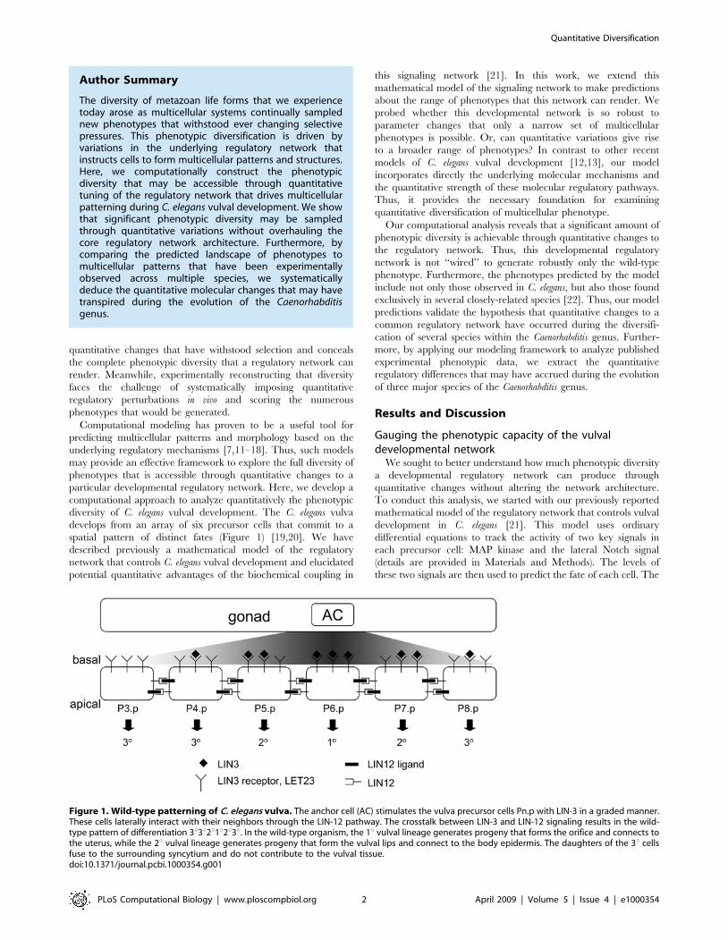
diversity of C. elegans vulval development. The C. elegans vulva

develops from an array of six precursor cells that commit to a

spatial pattern of distinct fates (Figure 1) [19,20]. We have

described previously a mathematical model of the regulatory

network that controls C. elegans vulval development and elucidated

potential quantitative advantages of the biochemical coupling in

this signaling network [21]. In this work, we extend this

mathematical model of the signaling network to make predictions

about the range of phenotypes that this network can render. We

probed whether this developmental network is so robust to

parameter changes that only a narrow set of multicellular

phenotypes is possible. Or, can quantitative variations give rise

to a broader range of phenotypes? In contrast to other recent

models of C. elegans vulval development [12,13], our model

incorporates directly the underlying molecular mechanisms and

the quantitative strength of these molecular regulatory pathways.

Thus, it provides the necessary foundation for examining

quantitative diversification of multicellular phenotype.

Our computational analysis reveals that a significant amount of

phenotypic diversity is achievable through quantitative changes to

the regulatory network. Thus, this developmental regulatory

network is not ‘‘wired’’ to generate robustly only the wild-type

phenotype. Furthermore, the phenotypes predicted by the model

include not only those observed in C. elegans, but also those found

exclusively in several closely-related species [22]. Thus, our model

predictions validate the hypothesis that quantitative changes to a

common regulatory network have occurred during the diversifi-

cation of several species within the Caenorhabditis genus. Further-

more, by applying our modeling framework to analyze published

experimental phenotypic data, we extract the quantitative

regulatory differences that may have accrued during the evolution

of three major species of the Caenorhabditis genus.

Results and Discussion

Gauging the phenotypic capacity of the vulvaldevelopmental network

We sought to better understand how much phenotypic diversity

a developmental regulatory network can produce through

quantitative changes without altering the network architecture.

To conduct this analysis, we started with our previously reported

mathematical model of the regulatory network that controls vulval

development in C. elegans [21]. This model uses ordinary

differential equations to track the activity of two key signals in

each precursor cell: MAP kinase and the lateral Notch signal

(details are provided in Materials and Methods). The levels of

these two signals are then used to predict the fate of each cell. The

Author Summary

The diversity of metazoan life forms that we experiencetoday arose as multicellular systems continually samplednew phenotypes that withstood ever changing selectivepressures. This phenotypic diversification is driven byvariations in the underlying regulatory network thatinstructs cells to form multicellular patterns and structures.Here, we computationally construct the phenotypicdiversity that may be accessible through quantitativetuning of the regulatory network that drives multicellularpatterning during C. elegans vulval development. We showthat significant phenotypic diversity may be sampledthrough quantitative variations without overhauling thecore regulatory network architecture. Furthermore, bycomparing the predicted landscape of phenotypes tomulticellular patterns that have been experimentallyobserved across multiple species, we systematicallydeduce the quantitative molecular changes that may havetranspired during the evolution of the Caenorhabditisgenus.

Figure 1. Wild-type patterning of C. elegans vulva. The anchor cell (AC) stimulates the vulva precursor cells Pn.p with LIN-3 in a graded manner.These cells laterally interact with their neighbors through the LIN-12 pathway. The crosstalk between LIN-3 and LIN-12 signaling results in the wild-type pattern of differentiation 3u3u2u1u2u3u. In the wild-type organism, the 1u vulval lineage generates progeny that forms the orifice and connects tothe uterus, while the 2u vulval lineage generates progeny that form the vulval lips and connect to the body epidermis. The daughters of the 3u cellsfuse to the surrounding syncytium and do not contribute to the vulval tissue.doi:10.1371/journal.pcbi.1000354.g001

Quantitative Diversification


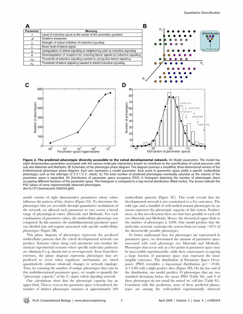
model consists of eight dimensionless parameters whose values

influence the pattern of fate choices (Figure 2A). To determine the

phenotypes that are accessible through quantitative modulation of

the network, we allowed each parameter to vary across a broad

range of physiological values (Materials and Methods). For each

combination of parameter values, the multicellular phenotype was

computed. In this manner, the multidimensional parameter space

was divided into sub-regions associated with specific multicellular

phenotypes (Figure 2B).

This phase diagram of phenotypes represents the predicted

multicellular patterns that the vulval developmental network can

produce. Extreme values along each parameter axis emulate the

classical experimental scenario where specific molecular pathways

are eliminated (e.g., knock out) or overexpressed. Away from these

extremes, the phase diagram represents phenotypes that are

predicted to occur when regulatory mechanisms are tuned

quantitatively without wholesale changes to network topology.

Thus, by counting the number of unique phenotypes that exist in

this multidimensional parameter space, we sought to quantify the

‘‘phenotypic capacity’’ of the C. elegans vulval signaling network.

Our calculations show that the phenotypic capacity has an

upper limit. That is, even as the parameter space is broadened, the

number of distinct phenotypes saturates at approximately 560

multicellular patterns (Figure 2C). This result reveals that the

developmental network is not constrained to a few outcomes. The

wild type and a handful of well-studied mutant phenotypes by no

means represent the phenotypic capacity of this system. Further-

more, in this six-cell system there are four fates possible to each cell

(see Materials and Methods). Hence, the theoretical upper limit to

the number of phenotypes is 4,096. Our model predicts that the

molecular network constrains the system from accessing ,85% of

the theoretically possible phenotypes.

To better understand how the phenotypes are represented in

parameter space, we determined the amount of parameter space

associated with each phenotype (see Materials and Methods).

Phenotypes that occur only at a few points in parameter space may

be inaccessible experimentally, while their counterparts occupying

a large fraction of parameter space may represent the more

tangible outcomes. The distribution of Parameter Space Occu-

pancy (PSO) resembles a log-normal distribution (m= 219.60,

s= 4.90) with a slight positive skew (Figure 2D). On the low end of

the distribution, our model predicts 19 phenotypes that are two

standard deviations below the mean PSO (Table S4), and 9 of

these phenotypes do not entail the mixed ‘m’ cell fate (Table S1).

Consistent with this prediction, none of these predicted pheno-

types are among the well-studied experimentally observed

Figure 2. The predicted phenotypic diversity accessible to the vulval developmental network. (A) Model parameters. The model haseight dimensionless parameters associated with the various molecular interactions known to contribute to the specification of vulval precursor cells(see also Materials and Methods). (B) Schematic of the phenotype phase diagram. This diagram portrays a simplified, three-dimensional version of the8-dimensional phenotype phase diagram. Each axis represents a model parameter. Each point in parameter space yields a specific multicellularphenotype, such as the wild-type (3u3u2u1u2u3u, black). (C) The total number of predicted phenotypes eventually saturates as the volume of theparameter space is expanded. (D) Distribution of parameter space occupancy (PSO). A histogram depicting the number of phenotypes (bars)occupying different fractions of the parameter space. This histogram is compared to a log-normal distribution (filled circles). The arrows indicate thePSO values of some experimentally observed phenotypes.doi:10.1371/journal.pcbi.1000354.g002



phenotypes. These highly unlikely outcomes reduce our evaluation

of the overall phenotypic capacity of this system.

Meanwhile, on the other end of the distribution, a small subset

of phenotypes occupies a disproportionately large portion of the

parameter space (Figure 2D). Within the positive skew is the wild-

type phenotype, consistent with a previous study that showed that

the developmental segment polarity network robustly produces the

wild-type multicellular pattern [7]. Extending beyond the wild-

type phenotype, our model predicts an additional 33 phenotypes

with PSO values that are two standard deviations above the mean

(see Table S5 for a list of these phenotypes), 25 of which do not

entail the mixed ‘m’ cell fate. These phenotypes are highly

represented in parameter space and suggest that significant

phenotypic diversity may be sampled by tuning quantitatively a

common underlying regulatory network. In fact, consistent with

model predictions, several of these 25 phenotypes have been

observed in C. elegans genetics experiments [23,24]. However, 10 of

these 25 phenotypes have not been reported and are novel

predicted phenotypes for future experimental validation.

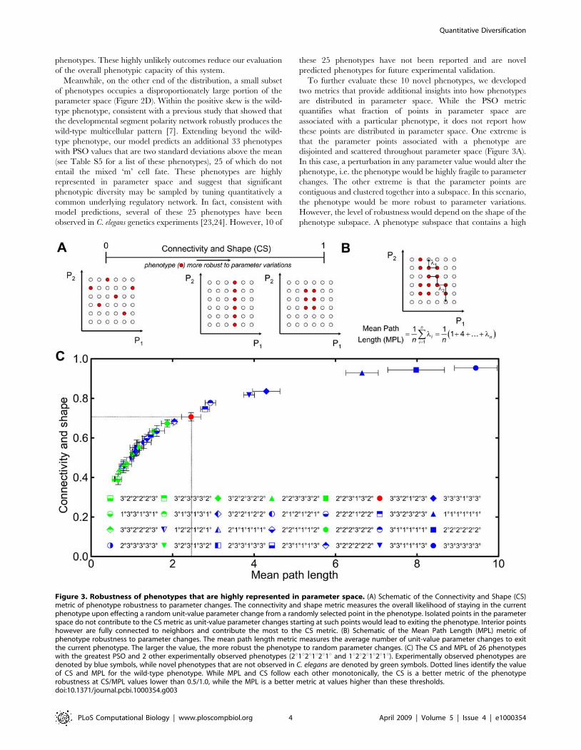
To further evaluate these 10 novel phenotypes, we developed

two metrics that provide additional insights into how phenotypes

are distributed in parameter space. While the PSO metric

quantifies what fraction of points in parameter space are

associated with a particular phenotype, it does not report how

these points are distributed in parameter space. One extreme is

that the parameter points associated with a phenotype are

disjointed and scattered throughout parameter space (Figure 3A).

In this case, a perturbation in any parameter value would alter the

phenotype, i.e. the phenotype would be highly fragile to parameter

changes. The other extreme is that the parameter points are

contiguous and clustered together into a subspace. In this scenario,

the phenotype would be more robust to parameter variations.

However, the level of robustness would depend on the shape of the

phenotype subspace. A phenotype subspace that contains a high

Figure 3. Robustness of phenotypes that are highly represented in parameter space. (A) Schematic of the Connectivity and Shape (CS)metric of phenotype robustness to parameter changes. The connectivity and shape metric measures the overall likelihood of staying in the currentphenotype upon effecting a random unit-value parameter change from a randomly selected point in the phenotype. Isolated points in the parameterspace do not contribute to the CS metric as unit-value parameter changes starting at such points would lead to exiting the phenotype. Interior pointshowever are fully connected to neighbors and contribute the most to the CS metric. (B) Schematic of the Mean Path Length (MPL) metric ofphenotype robustness to parameter changes. The mean path length metric measures the average number of unit-value parameter changes to exitthe current phenotype. The larger the value, the more robust the phenotype to random parameter changes. (C) The CS and MPL of 26 phenotypeswith the greatest PSO and 2 other experimentally observed phenotypes (2u1u2u1u2u1u and 1u2u2u1u2u1u). Experimentally observed phenotypes aredenoted by blue symbols, while novel phenotypes that are not observed in C. elegans are denoted by green symbols. Dotted lines identify the valueof CS and MPL for the wild-type phenotype. While MPL and CS follow each other monotonically, the CS is a better metric of the phenotyperobustness at CS/MPL values lower than 0.5/1.0, while the MPL is a better metric at values higher than these thresholds.doi:10.1371/journal.pcbi.1000354.g003



fraction of points at the ‘‘surface’’ (i.e., borders parameter points

belonging to another phenotype) would be less robust than a

phenotype where all its parameter points are tightly packed into a

subspace with minimal exposure to other phenotypes.

To capture these aspects of how parameter points of a particular

phenotype are distributed in parameter space, we developed a

Connectivity and Shape (CS) metric (Materials and Methods). The

value of the CS metric is bounded between 0 and 1 and represents

the average likelihood that for any point in phenotype subspace, a

unit change in any single parameter value maintains the

phenotype (Figure 3A). Thus, a CS value of 0 would refer to a

highly fragile phenotype whose points in parameter space are

‘‘isolated’’ or surrounded by other phenotypes. In contrast, a CS

value of near 1 would refer to a highly robust phenotype for which

most of the points in its parameter subspace are surrounded by

other points associated with the same phenotype. As a comple-

mentary approach to gauge the robustness of a phenotype to

parameter changes, we quantified the Mean Path Length (MPL) as

the average number of unit changes or ‘‘jumps’’ in parameter

values needed to start from any point within a phenotype subspace

and land on a foreign phenotype (Figure 3B, Materials and

Methods)[25]. Large values of MPL indicate that many changes in

parameter values are needed to change phenotype, signifying a

highly robust phenotype.

We calculated the MPL and CS metrics for the 26 phenotypes

with the highest PSO, including the wild-type phenotype

(Figure 3C). In addition, we computed these metrics for two

phenotypes (1u2u2u1u2u1u and 2u1u2u1u2u1u) that occupy less

parameter space (ranked 78th and 79th, respectively, in terms of

PSO, Figure 2D) but are well-established experimental outcomes.

Among these 28 phenotypes, our calculations show a high

correlation between MPL and CS, suggesting that these two

metrics are equivalent ways to gauge the robustness of a phenotype

to parameter variations. The model predicts seven phenotypes

with CS and MPL values greater than that of wild type. All seven

are experimentally observed in C. elegans, suggesting that

robustness, as quantified by these metrics, may be an important

determinant of experimental realizability. Meanwhile, there are 20

phenotypes with CS/MPL metrics lower than the wild type.

Among these 20, ten have been observed in C. elegans genetics

experiments, while the remaining 10 are the aforementioned novel

phenotypes that have not been observed in C. elegans. Notably, the

CS and MPL values of some of these novel phenotypes (e.g.,

2u2u2u3u2u2u, 3u2u2u3u2u2u, and 3u2u3u1u3u2u) falls within the

range of experimentally observed counterparts, suggesting that

these novel phenotypes may be the most realizable experimentally

upon performing the correct manipulations in the LIN-3/MAP

kinase and the LIN-12 pathways.

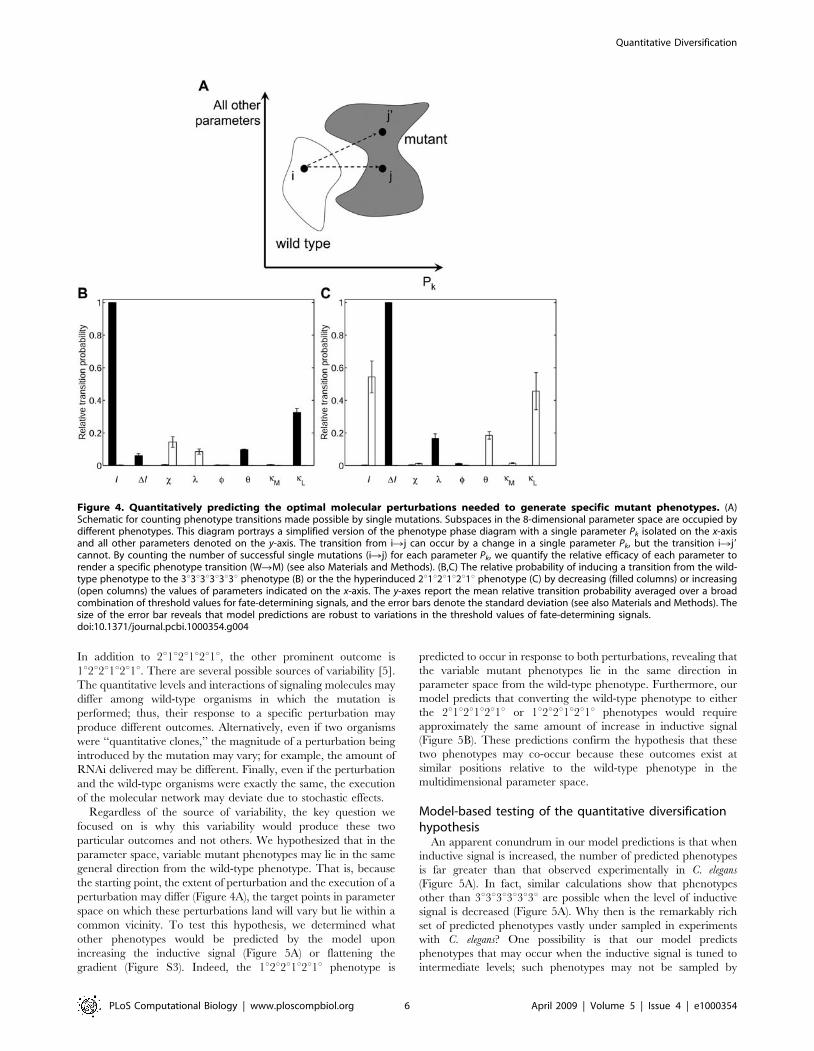
Identifying optimal molecular perturbations to renderspecific mutant phenotypes

Having predicted novel phenotypes and the experimental

realizability of these outcomes, a key question is how does one

render such phenotypes experimentally? The classical computa-

tional approach is to choose reference parameter values for the

wild-type phenotype and then to test the effect of specific

parameter perturbations. The choice of parameter perturbation

is motivated typically by a corresponding mutation that has been

performed experimentally with the goal of determining whether

the predicted phenotype matches the experimental outcome. The

pitfall, however, is that suitable reference parameter values for the

in vivo biochemistry of signaling pathways in live worms are

unknown. Furthermore, worms are not quantitative clones, and

each worm is likely to differ in its parametric settings. Finally, the

execution of a particular experimental perturbation is unlikely to

be realized in the same quantitative manner in each worm in every

trial.

Based on these considerations, we take a different approach that

is enabled by the phase diagram of phenotypes that we have

computed for this system. Using this phase diagram, we determine

all possible single-parameter changes (i.e., single mutations) that

successfully transition the wild-type phenotype into a mutant

phenotype of interest. The fraction of these successful single-

parameter changes that is associated with a particular parameter

reveals the relative efficacy with which that parameter perturba-

tion ‘‘transitions’’ the wild-type phenotype into the mutant

outcome (Figure 4A and Materials and Methods). In this manner,

these computations yield a transition probability that an increase

(or decrease) in each parameter will shift the phenotype from wild

type to a mutant pattern. Parameter changes with a higher

transition probability have a greater likelihood of generating the

desired mutant phenotype. Thus, this approach is the computa-

tional equivalent of a random genetic screen that evaluates all

possible mutations to determine the most effective ones that lead to

the mutant phenotype of interest.

To test initially this approach, we applied it to mutant

phenotypes that have been well established by genetics experi-

ments in C. elegans. We first predicted the best single-parameter

changes needed to transform the wild-type organism into a

vulvaless mutant. Vulvaless phenotypes have been observed in

genetics experiments and occur when all vulval precursor cells

acquire the 3u fate [2,24,26]. Our model predicts that the best way

to render the 3u3u3u3u3u3u phenotype is by decreasing the level of

inductive signaling (Figure 4B). This prediction is consistent with

experiments in which anchor cell ablation yields the uninduced all-

3u fate pattern [27].

In the other extreme of phenotypes, mutant worms with

multiple vulvae have been observed when the inductive signaling

pathway is hyperactivated [28–30]. In these mutants, the vulval

precursor cells acquire an intriguing alternating pattern of

2u1u2u1u2u1u where each 1u cell produces an invagination [31].

Consistent with this experimental observation, the model predicts

an increase in inductive signal as one of the most prominent ways

to yield this alternating phenotype (Figure 4C).

In addition, because all possible single mutations are evaluated,

our model analysis predicts additional ‘‘equivalent mutations’’ that

would render the same 2u1u2u1u2u1u phenotypic outcome

(Figure 4C). One of these equivalent mutations is to flatten the

gradient in soluble inductive factor (Figure 4C). This particular

prediction is remarkably consistent with what has been recently

uncovered about the most classical experimental mutation to yield

this phenotype. The loss of lin-15 has been shown to cause the

secretion of LIN-3 from the surrounding cells, an event that would

ablate the gradient [32]. A second equivalent mutation predicted

by the model is an increase in the threshold of lateral signaling

needed to inhibit the MAP kinase pathway (kL). This prediction

for generating a well-established phenotype through a non-

canonical perturbation is testable experimentally by decreasing

the binding affinity of the lateral signaling transcription complex

(LAG-1:LIN-12-cyto) to LBS elements in the cis-regulatory regions

of the genes that negatively regulate inductive signaling (ark-1, lip-

1, lst-1,2,3,4) [33]. This mutation would require greater lateral

signaling to inhibit the inductive MAP kinase pathway and would

be an indirect way to inflate the inductive signaling activity,

conceptually consistent with the direct hyperactivation of the

inductive signaling pathway.

An intriguing feature of mutants, such as lin-15(lf) [24,31] and

let-60(gf) [34], is that the observed multicellular pattern is variable.



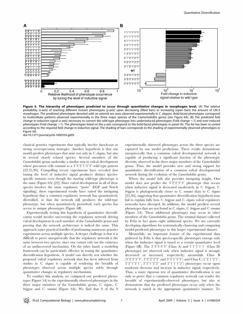
In addition to 2u1u2u1u2u1u, the other prominent outcome is

1u2u2u1u2u1u. There are several possible sources of variability [5].

The quantitative levels and interactions of signaling molecules may

differ among wild-type organisms in which the mutation is

performed; thus, their response to a specific perturbation may

produce different outcomes. Alternatively, even if two organisms

were ‘‘quantitative clones,’’ the magnitude of a perturbation being

introduced by the mutation may vary; for example, the amount of

RNAi delivered may be different. Finally, even if the perturbation

and the wild-type organisms were exactly the same, the execution

of the molecular network may deviate due to stochastic effects.

Regardless of the source of variability, the key question we

focused on is why this variability would produce these two

particular outcomes and not others. We hypothesized that in the

parameter space, variable mutant phenotypes may lie in the same

general direction from the wild-type phenotype. That is, because

the starting point, the extent of perturbation and the execution of a

perturbation may differ (Figure 4A), the target points in parameter

space on which these perturbations land will vary but lie within a

common vicinity. To test this hypothesis, we determined what

other phenotypes would be predicted by the model upon

increasing the inductive signal (Figure 5A) or flattening the

gradient (Figure S3). Indeed, the 1u2u2u1u2u1u phenotype is

predicted to occur in response to both perturbations, revealing that

the variable mutant phenotypes lie in the same direction in

parameter space from the wild-type phenotype. Furthermore, our

model predicts that converting the wild-type phenotype to either

the 2u1u2u1u2u1u or 1u2u2u1u2u1u phenotypes would require

approximately the same amount of increase in inductive signal

(Figure 5B). These predictions confirm the hypothesis that these

two phenotypes may co-occur because these outcomes exist at

similar positions relative to the wild-type phenotype in the

multidimensional parameter space.

Model-based testing of the quantitative diversificationhypothesis

An apparent conundrum in our model predictions is that when

inductive signal is increased, the number of predicted phenotypes

is far greater than that observed experimentally in C. elegans

(Figure 5A). In fact, similar calculations show that phenotypes

other than 3u3u3u3u3u3u are possible when the level of inductive

signal is decreased (Figure 5A). Why then is the remarkably rich

set of predicted phenotypes vastly under sampled in experiments

with C. elegans? One possibility is that our model predicts

phenotypes that may occur when the inductive signal is tuned to

intermediate levels; such phenotypes may not be sampled by

Figure 4. Quantitatively predicting the optimal molecular perturbations needed to generate specific mutant phenotypes. (A)Schematic for counting phenotype transitions made possible by single mutations. Subspaces in the 8-dimensional parameter space are occupied bydifferent phenotypes. This diagram portrays a simplified version of the phenotype phase diagram with a single parameter Pk isolated on the x-axisand all other parameters denoted on the y-axis. The transition from iRj can occur by a change in a single parameter Pk, but the transition iRj9cannot. By counting the number of successful single mutations (iRj) for each parameter Pk, we quantify the relative efficacy of each parameter torender a specific phenotype transition (WRM) (see also Materials and Methods). (B,C) The relative probability of inducing a transition from the wild-type phenotype to the 3u3u3u3u3u3u phenotype (B) or the the hyperinduced 2u1u2u1u2u1u phenotype (C) by decreasing (filled columns) or increasing(open columns) the values of parameters indicated on the x-axis. The y-axes report the mean relative transition probability averaged over a broadcombination of threshold values for fate-determining signals, and the error bars denote the standard deviation (see also Materials and Methods). Thesize of the error bar reveals that model predictions are robust to variations in the threshold values of fate-determining signals.doi:10.1371/journal.pcbi.1000354.g004



classical genetics experiments that typically involve knock-out or

strong overexpression strategies. Another hypothesis is that our

model predicts phenotypes that arise not only in C. elegans, but also

in several closely related species. Several members of the

Caenorhabditis genus undertake a similar step in vulval development

where precursor cells commit to a 3u3u2u1u2u3u wild type pattern

[22,35,36]. Compelling recent experiments have revealed that

tuning the level of inductive signal produces distinct species-

specific mutants even though the starting wild-type phenotype is

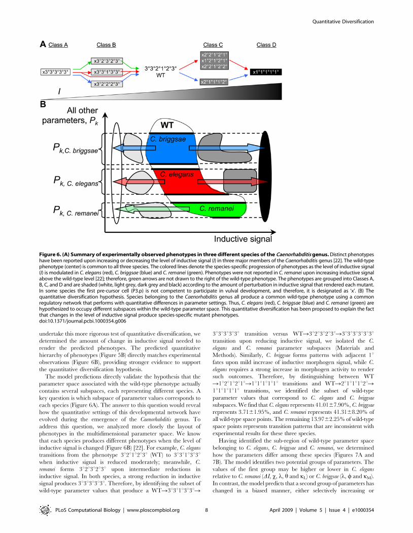
the same (Figure 6A) [22]. Since vulval development in all of these

species involves the same regulatory ‘‘parts’’ (EGF and Notch

signaling), these experimental results have raised the intriguing

hypothesis that a common regulatory network has quantitatively

diversified, so that the network still produces the wild-type

phenotype, but when quantitatively perturbed, each species has

access to unique phenotypes (Figure 6B).

Experimentally testing this hypothesis of quantitative diversifi-

cation would involve uncovering the regulatory network driving

vulval development in each member of the Caenorhabditis genus and

proving that the network architecture is indeed the same. This

approach raises practical hurdles of performing numerous genetics

experiments across multiple species. A deeper challenge is that it is

difficult to prove unequivocally that the regulatory network is the

same between two species, since one cannot rule out the existence

of an undiscovered mechanism. On the other hand, a modeling

framework can be particularly effective in testing the quantitative

diversification hypothesis. A model can directly test whether the

proposed vulval regulatory network that has been inferred from

studies in C. elegans is capable of rendering the breadth of

phenotypes observed across multiple species solely through

quantitative changes in regulatory mechanisms.

To conduct this analysis, we compared our predicted pheno-

types (Figure 5A) to the experimentally observed phenotypes in the

three major members of the Caenorhabditis genus, C. elegans, C.

briggsae and C. remanei (Figure 6A). We find that 8 of the 9

experimentally observed phenotypes across the three species are

captured by our model predictions. These results demonstrate

unequivocally that a common vulval developmental network is

capable of producing a significant fraction of the phenotypic

diversity observed in the three major members of the Caenorhabditis

genus. Thus, the model provides new and strong support for

quantitative diversification of a common vulval developmental

network during the evolution of the Caenorhabditis genus.

Where the model fails also provides intriguing insight. Our

model does not predict the 3u2u2u2u3u phenotype that occurs

when inductive signal is decreased moderately in C. briggsae. C.

briggsae is phylogenetically closer to C. remanei than to C. elegans

[22,36], suggesting that quantitative diversification hypothesis may

fail to explain fully how C. briggsae and C. elegans vulval regulatory

networks have diverged. In addition, the model predicts several

phenotypes that are not found in C. elegans, C. briggsae and C. remanei

(Figure 5A). These additional phenotypes may occur in other

members of the Caenorhabditis genus. The seminal dataset collected

by Felix in fact spans eight additional species. We are currently

developing algorithms for systematically clustering and comparing

model-predicted phenotypes to this larger experimental dataset.

Meanwhile, an important feature of the experimental data

gathered by Felix is that species-specific phenotypes emerge only

when the inductive signal is tuned to a certain quantitative level

(Figure 6B). The 3u3u3u3u3u (Class A) and 1u1u1u1u1u (Class D)

phenotypes are observed only when inductive signal is strongly

decreased or increased, respectively; meanwhile Class B

(3u2u3u2u3u, 3u2u2u2u3u and 3u3u1u3u3u) and Class C (1u2u1u2u1u,2u2u1u2u1u, 2u2u1u2u2u and 2u1u1u1u2u) phenotypes occur upon

moderate decrease and increase in inductive signal, respectively.

Thus, a more rigorous test of quantitative diversification is not

only to prove that a common regulatory network can render the

breadth of experimentally-observed phenotypes, but also to

demonstrate that the predicted phenotypes occur only when the

network is tuned in the appropriate quantitative manner. To

Figure 5. The hierarchy of phenotypes predicted to occur through quantitative changes in morphogen level. (A) The relativeprobability (x-axis) of reaching different mutant phenotypes (y-axis) upon decreasing (filled bars) or increasing (open bars) the amount of LIN-3morphogen. The predicted phenotypes denoted with an asterisk are ones observed experimentally in C. elegans. Bold-faced phenotypes correspondto multicellular patterns observed experimentally in the three major species of the Caenorhabditis genus (see Figure 6A). (B) The predicted foldchange in inductive signal (x-axis) necessary to convert the wild-type phenotype into underinduced phenotypes (Fold change ,1) and over-inducedphenotypes (Fold change .1). The phenotypes listed on the y-axis correspond to the bold-faced phenotypes in panel (A). The list has been re-sortedaccording to the required fold change in inductive signal. The shading of bars corresponds to the shading of experimentally observed phenotypes inFigure 6A.doi:10.1371/journal.pcbi.1000354.g005



undertake this more rigorous test of quantitative diversification, we

determined the amount of change in inductive signal needed to

render the predicted phenotypes. The predicted quantitative

hierarchy of phenotypes (Figure 5B) directly matches experimental

observations (Figure 6B), providing stronger evidence to support

the quantitative diversification hypothesis.

The model predictions directly validate the hypothesis that the

parameter space associated with the wild-type phenotype actually

contains several subspaces, each representing different species. A

key question is which subspace of parameter values corresponds to

each species (Figure 6A). The answer to this question would reveal

how the quantitative settings of this developmental network have

evolved during the emergence of the Caenorhabditis genus. To

address this question, we analyzed more closely the layout of

phenotypes in the multidimensional parameter space. We know

that each species produces different phenotypes when the level of

inductive signal is changed (Figure 6B) [22]. For example, C. elegans

transitions from the phenotype 3u2u1u2u3u (WT) to 3u3u1u3u3uwhen inductive signal is reduced moderately; meanwhile, C.

remanei forms 3u2u3u2u3u upon intermediate reductions in

inductive signal. In both species, a strong reduction in inductive

signal produces 3u3u3u3u3u. Therefore, by identifying the subset of

wild-type parameter values that produce a WTR3u3u1u3u3uR

3u3u3u3u3u transition versus WTR3u2u3u2u3uR3u3u3u3u3u3utransition upon reducing inductive signal, we isolated the C.

elegans and C. remanei parameter subspaces (Materials and

Methods). Similarly, C. briggsae forms patterns with adjacent 1ufates upon mild increase of inductive morphogen signal, while C.

elegans requires a strong increase in morphogen activity to render

such outcomes. Therefore, by distinguishing between WT

R1u2u1u2u1uR1u1u1u1u1u transitions and WTR2u1u1u1u2uR1u1u1u1u1u transitions, we identified the subset of wild-type

parameter values that correspond to C. elegans and C. briggsae

subspaces. We find that C. elegans represents 41.0167.90%, C. briggsae

represents 3.7161.95%, and C. remanei represents 41.3168.20% of

all wild-type space points. The remaining 13.9762.25% of wild-type

space points represents transition patterns that are inconsistent with

experimental results for these three species.

Having identified the sub-region of wild-type parameter space

belonging to C. elegans, C. briggsae and C. remanei, we determined

how the parameters differ among these species (Figures 7A and

7B). The model identifies two potential groups of parameters. The

values of the first group may be higher or lower in C. elegans

relative to C. remanei (DI, x, l, h and kL) or C. briggsae (l, w and kM).

In contrast, the model predicts that a second group of parameters has

changed in a biased manner, either selectively increasing or

Figure 6. (A) Summary of experimentally observed phenotypes in three different species of the Caenorhabditis genus. Distinct phenotypeshave been reported upon increasing or decreasing the level of inductive signal (I) in three major members of the Caenorhabditis genus [22]. The wild-typephenotype (center) is common to all three species. The colored lines denote the species-specific progression of phenotypes as the level of inductive signal(I) is modulated in C. elegans (red), C. briggsae (blue) and C. remanei (green). Phenotypes were not reported in C. remanei upon increasing inductive signalabove the wild-type level [22]; therefore, green arrows are not drawn to the right of the wild-type phenotype. The phenotypes are grouped into Classes A,B, C, and D and are shaded (white, light grey, dark grey and black) according to the amount of perturbation in inductive signal that rendered each mutant.In some species the first pre-cursor cell (P3.p) is not competent to participate in vulval development, and therefore, it is designated as ‘x’. (B) Thequantitative diversification hypothesis. Species belonging to the Caenorhabditis genus all produce a common wild-type phenotype using a commonregulatory network that performs with quantitative differences in parameter settings. Thus, C. elegans (red), C. briggsae (blue) and C. remanei (green) arehypothesized to occupy different subspaces within the wild-type parameter space. This quantitative diversification has been proposed to explain the factthat changes in the level of inductive signal produce species-specific mutant phenotypes.doi:10.1371/journal.pcbi.1000354.g006



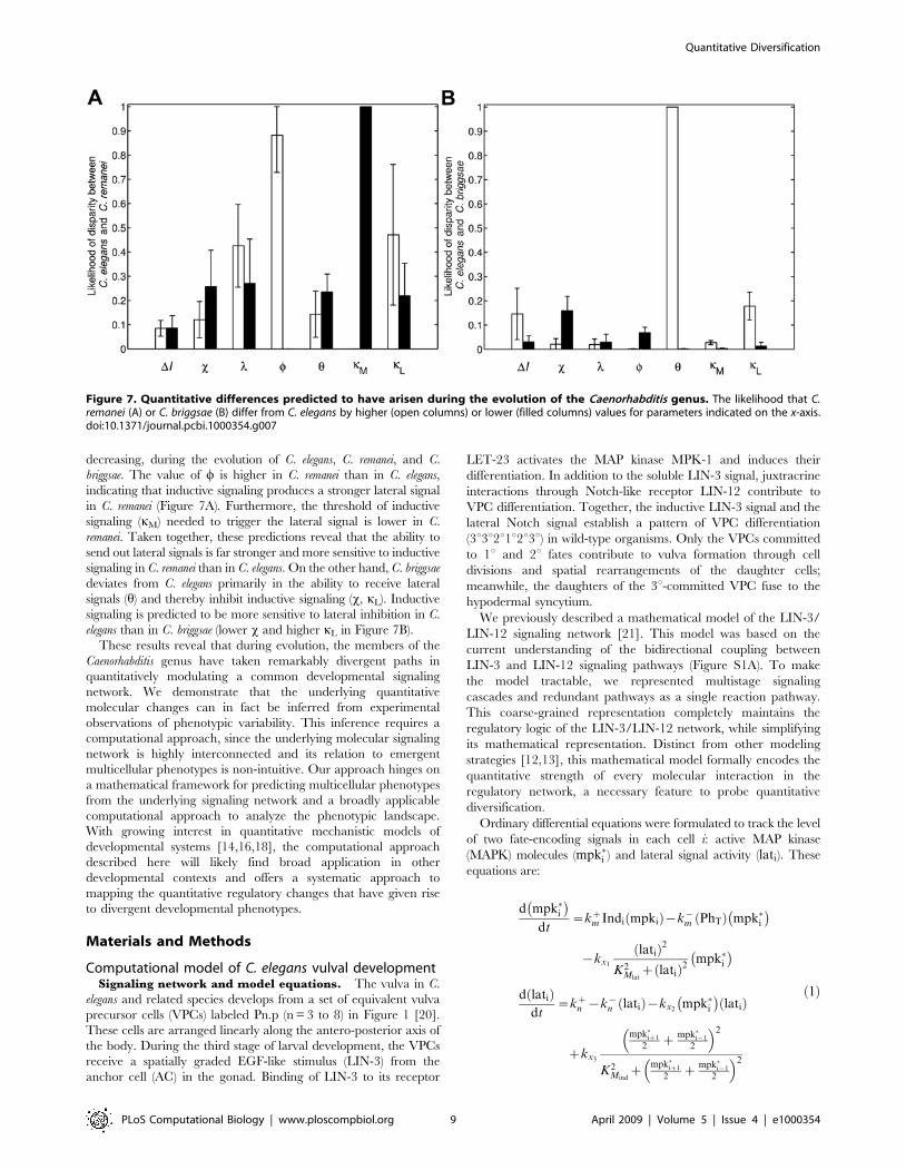
decreasing, during the evolution of C. elegans, C. remanei, and C.

briggsae. The value of w is higher in C. remanei than in C. elegans,

indicating that inductive signaling produces a stronger lateral signal

in C. remanei (Figure 7A). Furthermore, the threshold of inductive

signaling (kM) needed to trigger the lateral signal is lower in C.

remanei. Taken together, these predictions reveal that the ability to

send out lateral signals is far stronger and more sensitive to inductive

signaling in C. remanei than in C. elegans. On the other hand, C. briggsae

deviates from C. elegans primarily in the ability to receive lateral

signals (h) and thereby inhibit inductive signaling (x, kL). Inductive

signaling is predicted to be more sensitive to lateral inhibition in C.

elegans than in C. briggsae (lower x and higher kL in Figure 7B).

These results reveal that during evolution, the members of the

Caenorhabditis genus have taken remarkably divergent paths in

quantitatively modulating a common developmental signaling

network. We demonstrate that the underlying quantitative

molecular changes can in fact be inferred from experimental

observations of phenotypic variability. This inference requires a

computational approach, since the underlying molecular signaling

network is highly interconnected and its relation to emergent

multicellular phenotypes is non-intuitive. Our approach hinges on

a mathematical framework for predicting multicellular phenotypes

from the underlying signaling network and a broadly applicable

computational approach to analyze the phenotypic landscape.

With growing interest in quantitative mechanistic models of

developmental systems [14,16,18], the computational approach

described here will likely find broad application in other

developmental contexts and offers a systematic approach to

mapping the quantitative regulatory changes that have given rise

to divergent developmental phenotypes.

Materials and Methods

Computational model of C. elegans vulval developmentSignaling network and model equations. The vulva in C.

elegans and related species develops from a set of equivalent vulva

precursor cells (VPCs) labeled Pn.p (n = 3 to 8) in Figure 1 [20].

These cells are arranged linearly along the antero-posterior axis of

the body. During the third stage of larval development, the VPCs

receive a spatially graded EGF-like stimulus (LIN-3) from the

anchor cell (AC) in the gonad. Binding of LIN-3 to its receptor

LET-23 activates the MAP kinase MPK-1 and induces their

differentiation. In addition to the soluble LIN-3 signal, juxtracrine

interactions through Notch-like receptor LIN-12 contribute to

VPC differentiation. Together, the inductive LIN-3 signal and the

lateral Notch signal establish a pattern of VPC differentiation

(3u3u2u1u2u3u) in wild-type organisms. Only the VPCs committed

to 1u and 2u fates contribute to vulva formation through cell

divisions and spatial rearrangements of the daughter cells;

meanwhile, the daughters of the 3u-committed VPC fuse to the

hypodermal syncytium.

We previously described a mathematical model of the LIN-3/

LIN-12 signaling network [21]. This model was based on the

current understanding of the bidirectional coupling between

LIN-3 and LIN-12 signaling pathways (Figure S1A). To make

the model tractable, we represented multistage signaling

cascades and redundant pathways as a single reaction pathway.

This coarse-grained representation completely maintains the

regulatory logic of the LIN-3/LIN-12 network, while simplifying

its mathematical representation. Distinct from other modeling

strategies [12,13], this mathematical model formally encodes the

quantitative strength of every molecular interaction in the

regulatory network, a necessary feature to probe quantitative

diversification.

Ordinary differential equations were formulated to track the level

of two fate-encoding signals in each cell i: active MAP kinase

(MAPK) molecules (mpk�i ) and lateral signal activity (lati). These

equations are:

d mpk�i� �

dt~kz

m Indi mpkið Þ{k{m PhTð Þ mpk�i

� �

{kx1

latið Þ2

K2Mlat

z latið Þ2mpk�i� �

d latið Þdt

~kzn {k{

n latið Þ{kx2mpk�i� �

latið Þ

zkx3

mpk�iz1

2z

mpk�i{1

2

� �2

K2Mind

zmpk�iz1

2z

mpk�i{1

2

� �2

ð1Þ

Figure 7. Quantitative differences predicted to have arisen during the evolution of the Caenorhabditis genus. The likelihood that C.remanei (A) or C. briggsae (B) differ from C. elegans by higher (open columns) or lower (filled columns) values for parameters indicated on the x-axis.doi:10.1371/journal.pcbi.1000354.g007



where ni is the number of neighbors for cell i and the other

dimensional parameters are described in the legend to Figure S1A.

In addition, each VPC is stimulated by a local amount of

inductive signal, Indi. The values for Indi were determined by

modeling diffusive transport of the soluble factor coupled with

linear degradation in the extracellular space. At steady state, the

gradient is described by:

0~DL2 Ind½ �

Lx2{kd Ind½ �, ð2Þ

whose solution is:

Ind½ � xð Þ~ IndP6:p

� �e{

ffiffiffikdD

px, ð3Þ

when we require that Ind½ � x~0ð Þ~ IndP6:p

� �. We rewrite this

solution by rescaling the spatial axis, x, in terms of the length of

P3.p-P6.p VPC field, L, as follows:

Ind½ � ~xxð Þ~ IndP6:p

� �e{

ffiffiffikdD

pL2

~xx3~ IndP6:p

� �DI

~xx3, ð4Þ

where ~xx is 0, 1, 2 and 3 for P6.p, P5/7.p, P4/8.p and P3.p,

respectively. Thus, the parameters IndP6.p and DI specify the local

level of inductive signal (Indi). A change in the value of DI alters

the steepness of the exponential gradient in inductive signal.

The dimensional variables mpk�i and lati were normalized by

their characteristic values, mpkT and latT, respectively to yield the

following nondimensional state variables:

mi~mpk�impkT

, li~lati

latT: ð5Þ

Subsequently, dimensional parameters in the model equations

were rearranged to identify the following dimensionless parameter

groups:

t~k{m PhTð Þt, I~

kzm IndP6:p

� �k{

m PhTð Þ , x~kx1

k{m PhTð Þ ,

l~kz

n

k{n latTð Þ , w~

kx3

k{n latTð Þ , h~

kx2mpkTð Þk{

n

,

kM~KMind

mpkT, kL~

KMlat

latT, c~

k{n

k{m PhTð Þ :

ð6Þ

Thus, by using non-dimensional parameters, we have reduced

the space of parameters from 13 dimensional parameters to 9

dimensionless ones. This reduction reduces the computational

load albeit this load is not prohibitive as others have analyzed

parameteric sensitivity of biomolecular networks by sweeping

across 36 dimensional parameters[37]. Using these nondimen-

sional quantities, our model equations may be rewritten as follows:

dmi

dt~ DIð Þ

~xx3I 1{mið Þ{mi{xmi

l2i

k2Lzl2

i

,

dli

dt~c l{li{hmilizw

mi{1

ni{1z miz1

niz1

� �2

k2Mz mi{1

ni{1z miz1

niz1

� �2

264

375:

ð7Þ

Framework for assigning cell fates. The timing of VPC

patterning has been studied by ablating the anchor cell (AC) at

different times during the induction process. Results from these

experiments have established that the AC (and therefore, the LIN-

3 signal that it secretes) is needed for approximately 6 hours in

order for the VPCs to commit to the 3u3u2u1u2u3u fate pattern

[26,27]. Our model calculations show that the fate-determining

signals (MAP kinase (mi) and lateral (li) signals) reach their steady-

state values within 5 hours for reference parameter values (detailed

below). Therefore, we worked under the reasonable assumption

that the steady-state values of mi and li prescribe the fate choice of

each VPC. For all simulations, the steady-state solution of the

dimensionless model equations was determined using the initial

condition that the levels of inductive and lateral signal are zero in

all cells. We note that for steady-state calculations the

dimensionless group c is eliminated from model equations (7).

The output of each simulation is the dimensionless magnitudes

of the fate-determining signals (mi, li). These are in turn recast into

the dimensional form (mpk�i , lati) from which fate assignments are

determined using the framework that we described previously

(Figure S1B) [21]. Briefly, (mpk�i , lati) in each VPC is a point in

the (mpk�, lat) fate plane. Two orthogonal thresholds, (mpk�Th,

latTh) segregate the fate plane into four quadrants. The

dimensional inductive and lateral signals in each cell are compared

against their respective threshold values, which then translate into

1u, 2u, 3u or m fate quadrants (Table S1).

Quantifying phenotypic capacityIn order to explore phenotypes that would result from

quantitative variations in network performance, we varied the

value of each dimensionless parameter, starting from its central

value and expanding in a step-wise fashion by increasing and

decreasing its value by ,3–4 fold. The central values of the

dimensionless parameters were determined as described in

Supporting Text S1. In this manner, the parameter space

hypervolume was expanded sequentially and contained 38, 58,

78, 98 and ultimately 118 points. Therefore, at its maximum size,

the parameter space contained 11 values per parameter (equally

spaced on a log scale), spanned 5–6 orders of magnitude for each

parameter (Tables S2, S3), and represented 118 parameter

combinations in total.

For each combination of 8 model parameter values, we

computed the fate pattern. Importantly, the fate of each cell i is

determined by whether the amounts of MAP kinase and lateral

signals in that cell (mpki and lati) exceed threshold levels (mpk�Th

and latTh, respectively; see Table S1). Because these threshold

values are unknown, and in fact, may be a source of variation in an

evolutionary context, we computed fate patterns across a broad

range of threshold values. Specifically, mpk�Th and latTh were

varied across the ranges 0ƒmpk�Thƒ10,000 molec=cell and

0ƒlatThƒ100,000 molec=cell, respectively. The cumulative

number of fates predicted across the 8-dimensional parameter

space for every combination of threshold values is reported in

Figure 2C.

Calculating the Parameter Space Occupancy (PSO)To quantify the PSO for each phenotype, we determined the

number of parameter points associated with each phenotype at

every combination of threshold values. This total level of

occurrence of each phenotype was divided by the total number

of parameter points to yield the fraction of parameter space

occupied by that particular phenotype. Phenotypes were binned

according to the fraction of parameter space occupied in unit log10

bins (i.e., 1 to 0.1, 0.1 to 0.01, etc). The number of distinct



phenotypes in each bin is plotted on the y-axis in Figure 2D. The

distribution of parameter space occupancy was then fit to a log-

normal probability distribution. There are 19 phenotypes two

standard deviations below the mean (Table S4) and 34 phenotypes

two standard deviations above the mean (Table S5).

Quantifying the robustness of the phenotype subspacesto parameter variations: the Connectivity and Shape (CS)and the Mean Path Length (MPL) metrics

Each point in the 8-dimensional parameter space maps to a

phenotype (Figure 2B). We refer to the collection of points in the

parameter space that are associated with a particular phenotype as

the phenotype subspace. To quantify the CS value for each

phenotype, we distinguished between isolated, edge, and interior

points in the phenotype subspace. Isolated points are those points

for which unit jumps along both (increase and decrease) directions

of every parameter axis lead to points associated with another

phenotype. In the other extreme, there are interior points for

which unit jumps in both directions along every parameter axis reach

points that still belongs to the same phenotype. Finally, between

these possibilities are edge points: a unit jump in at least one

direction along at least one parameter axis leads to another

phenotype. To calculate the CS metric for a phenotype, we assign

each point in the phenotype subspace a score equal to the number

of neighboring points that belong to the same phenotype. This

score ranges between 0 (for isolated points) and 16 (for interior

points). We add the scores of each point in the phenotype subspace

and normalize this total by the maximum possible score for the

phenotype space, accounting for edge effects due to finite

parameter domains. This normalized score is the CS value plotted

in Figure 3C.

A complementary approach to gauge robustness is to quantify

how easy it is to drift out of the phenotype subspace by computing

the MPL of escape from the phenotype subspace. We choose

randomly a point in the subspace and then make unit jumps along

a randomly selected parameter axis and direction. We record the

number of jumps taken before exiting the phenotype. This process

is repeated until the running average number of jumps stabilizes.

We conduct 10 such drift trial reseeding the random number

generator between trials. The mean path length is the average over

these 10 trials.

Importantly, the 8-dimensional phenotype phase diagram will

be sensitive to the threshold values of MAPK (mpk�Th) and lateral

(latTh) signals. Recall that these thresholds determine how fates are

assigned (Table S1). Hence, we computed the MPL and CS

metrics across 25 different threshold combinations spanning the

following ranges:

mpk�Th[ 1000,2000,3000,4000,5000½ � molecules=cell

latTh[ 10000,20000,30000,40000,50000½ � molecules=cell

Figure 3C reports the average and standard error across these 25

threshold combinations.

Predicting the most effective molecular perturbations forrendering mutant phenotypes: the transition probability

Each phenotype, including the wild type, occupies a subspace

within the 8-dimensional parameter space (Figure 2B). This phase

diagram of phenotypes was analyzed to address the following

question: given a choice of 8 single mutations (i.e., 8 parameter

perturbations), which single-parameter change (i.e., single muta-

tion) would be most likely to promote a transition from wild-type

(W) to a mutant (M) phenotype? To address this question, we rank

ordered the parameters according to their relative transition

probabilities (Figures 4B and 4C), computed as described below.

The same transition probability metric is computed to quantify the

single-parameter differences that distinguish C. elegans from closely

related species (Figures 7A and 7B). For this analysis, ‘‘transitions’’

between parameter spaces associated with C. elegans and another

species (C. briggsae or C. remanei) were considered.

For the purpose of this discussion, let Pk denote each

dimensionless parameter where k = 1 to 8. Let i denote a point

in the W parameter space, and j denote a point in the M-

parameter space (Figure 4A). By scanning through all (i, j) pairs,

we determined the total number that differ only by a single

parameter value. These pairs represent the cases where a single-

parameter change can cause a WRM phenotype transition.

Among this total number of single-mutation pairs, we determined

the fraction of phenotype transitions that are attributable to an

increase in a particular parameter Pk. This fraction is the transition

probability of WRM phenotype transition by increasing Pk. The

same calculation was conducted for quantifying the transition

probability due to a decrease in Pk.

To determine the robustness of the transition probability to

variations in the fate-determining thresholds, we computed the

transition probability for 25 different threshold combinations

presented above. Hence, the y-axes of Figures 4B, 4C, 7A, and 7B

report the mean transition probability computed over all these 25

threshold combinations, and the error bar denotes the standard

deviation.

Predicting the phenotypes accessible throughquantitative changes in the level of inductive signal

Starting from the wild-type phenotype, we determined all the

mutant phenotypes that may be rendered solely by increasing (or

decreasing) the inductive signal. Since some mutant phenotypes

are more prevalent than others, we quantified the likelihood that

an increase (or decrease) in inductive signal would produce each

mutant (M). To quantify this likelihood of phenotype occurrence,

we first tallied the total number of ways that a change in inductive

signal (I) would abolish the wild-type (W) phenotype. Among this

total, we quantified the fraction that shifted W to a specific mutant

M upon an increase (or decrease) in I. This fraction represents the

likelihood of producing M phenotype by an increase (or decrease)

in inductive signal (I).

Phenotype assignments must be sensitive to fate-determining

threshold values of MAPK and lateral signals (Table S1). To

quantify the robustness of the likelihood of phenotype occurrence

to threshold variations, we performed the calculation for 25

different threshold combinations (as described above). The mean

of the likelihood of phenotype occurrence is reported in Figure 5A

and Figure S2A, and the error bars denote the standard deviation.

Figure 5A shows the mutant phenotypes with the greatest

likelihood of phenotype occurrence upon an increase (empty) or

decrease (filled) in inductive signal. The more complete set of

phenotypes, including the ones that occur less frequently, are

shown in Figure S2A. Similar calculations were performed to

determine the phenotype diversity due to changes in gradient

steepness. Figure S3 shows the mutant phenotypes with greatest

likelihood of phenotype occurrence upon an increase (empty) and

decrease (filled) in gradient steepness. Note the occurrence of

1u2u2u1u2u1u and 2u1u2u1u2u1u phenotypes in both Figure 5A and

Figure S3.

In addition to the likelihood of generating a particular mutant

phenotype, it is also important to gauge the amount of change in

inductive signal needed to render each mutant. Some mutant



phenotypes may require only small changes, while others may

require substantial perturbations. Therefore, we quantified the

fold change in I needed to produce a specific mutant phenotype

(M). For every increase (or decrease) in I that produced phenotype

M, we kept track of the associated magnitude of change in I. The

geometric mean of these magnitudes was computed to give the

fold change in I. As with other calculations, we examined the

robustness of this quantity to variations in fate-determining

thresholds. The mean fold change in I across a broad range of

threshold settings is reported in Figure 5B and Figure S2B, and the

error bars represent the standard deviation.

Partitioning the wild-type subspace into species-specificregions

A key experimental observation is that changes in inductive

signal produce species-specific phenotypes [22]. Figure S4

highlights the progression of phenotypes observed in C. elegans,

C. briggsae, and C. remanei along the inductive signal axis. We

developed a computational approach to analyze how these

experimental phenotypes are arranged in our predicted phase

diagram of phenotypes with the goal of identifying the regions

within the wild-type subspace that belongs to each species.

First, we designated each phenotype with a letter code (Figure

S4), so that a string of characters or a word may be used to

represent the phenotype progression of each species. Phenotypes

that are not described in Figure S4 were designated ‘O’. For

example, following the lines for C. elegans in Figure S4, one word is

APWRD. Using this nomenclature, we identified the words that

are consistent with the fate progression observed experimentally in

C. elegans, C. briggsae, and C. remanei (Table S6).

Next, we determined the word associated with every predicted

point in the wild-type subspace. To construct the word, we varied

the value of I from its minimum to maximum while holding all

other parameter values constant. As the I-axis was traversed, we

recorded each phenotype with its character designation, thereby

yielding a 11-character word (11 characters because of the

discretization of the I-axis). The length of these words was then

condensed by eliminating adjacent repeats of a character. For

example, APPPOWOSSDD would become APOWOSD (Figure

S5). Since ‘O’ phenotypes include cases where VPCs are

designated as ‘m’ fate (a fate whose experimental equivalent

remains to be elucidated), we removed ‘O’ from the predicted

words. In the example, APOWOSD would become APWSD.

Thus, at the end of this step, every point in the wild-type

parameter is associated with a word that characterizes how the

phenotype would change when I is increased or decreased.

Finally, we compared the predicted words associated with each

point in wild-type parameter space with the experimentally

observed phenotype progressions/words of C. elegans, C. briggsae,

and C. remanei. In this manner, we identified the regions within the

wild-type parameter space associated with each species.

Supporting Information

Text S1 Rationale for the central values of dimensionless

parameters

Found at: doi:10.1371/journal.pcbi.1000354.s001 (0.32 MB PDF)

Figure S1 Model schematic of regulatory network and fate

assignments


Figure S2 Extended set of phenotypes that occur upon changing

the level of inductive signal


Figure S3 Phenotypic diversity caused by quantitative changes

in gradient steepness


Figure S4 Letter representations of the phenotypes observed in

C. elegans, C. briggsae and C. remanei


Figure S5 An illustration of our word representation for the

order of phenotypes that occurs as inductive signal is increased


Table S1 Fate assignment based on threshold values


Table S2 The values of dimensional parameters used to

determine the center values for the dimensionless parameters


Table S3 Range of values for dimensionless model parameters


Table S4 List of phenotypes with PSO values that are two

standard deviations below the mean


Table S5 List of phenotypes with PSO values that are two

standard deviations above the mean


Table S6 Characteristic words associated with each species


Author Contributions

Conceived and designed the experiments: CAG. Performed the experi-

ments: CAG. Analyzed the data: CAG PWS ARA. Contributed reagents/

materials/analysis tools: PWS. Wrote the paper: CAG ARA.

References

1. Nusslein-Volhard C, Wieschaus E (1980) Mutations affecting segment numberand polarity in Drosophila. Nature 287: 795–801.

2. Sulston JE, Horvitz HR (1981) Abnormal cell lineages in mutants of thenematode Caenorhabditis elegans. Dev Biol 82: 41–55.

3. Colman-Lerner A, Gordon A, Serra E, Chin T, Resnekov O, et al. (2005)

Regulated cell-to-cell variation in a cell-fate decision system. Nature 437: 699–706.

4. Elowitz MB, Levine AJ, Siggia ED, Swain PS (2002) Stochastic gene expression

in a single cell. Science 297: 1183–1186.

5. Samoilov MS, Price G, Arkin AP (2006) From fluctuations to phenotypes: the

physiology of noise. Sci STKE 2006: re17.

6. Volfson D, Marciniak J, Blake WJ, Ostroff N, Tsimring LS, et al. (2006) Originsof extrinsic variability in eukaryotic gene expression. Nature 439: 861–864.

7. von Dassow G, Meir E, Munro EM, Odell GM (2000) The segment polaritynetwork is a robust developmental module. Nature 406: 188–192.

8. Meir E, von Dassow G, Munro E, Odell GM (2002) Robustness, flexibility, and

the role of lateral inhibition in the neurogenic network. Curr Biol 12: 778–786.

9. Abzhanov A, Protas M, Grant BR, Grant PR, Tabin CJ (2004) Bmp4 and

morphological variation of beaks in Darwin’s finches. Science 305: 1462–1465.

10. Doebley J, Stec A, Hubbard L (1997) The evolution of apical dominance in

maize. Nature 386: 485–488.

11. Amonlirdviman K, Khare N, Tree D, Chen W, Axelrod JD, et al. (2005)

Mathematical modeling of planar cell polarity to understand domineering

nonautomony. Science 307: 423–426.

12. Fisher J, Piterman N, Hajnal A, Henzinger TA (2007) Predictive modeling of

signaling crosstalk during C. elegans vulval development. PLoS Comput Biol 3: e92.

13. Fisher J, Piterman N, Hubbard EJ, Stern MJ, Harel D (2005) Computational

insights into Caenorhabditis elegans vulval development. Proc Natl Acad

Sci U S A 102: 1951–1956.

14. Giurumescu CA, Asthagiri AR (2007) Signal Processing during Developmental

Multicellular Patterning. Biotechnol Prog.

15. Pribyl M, Muratov CB, Shvartsman SY (2003) Transitions in the model of

epithelial patterning. Dev Dynamics 226: 155–159.



16. Reeves GT, Muratov CB, Schupbach T, Shvartsman SY (2006) Quantitative

models of developmental pattern formation. Dev Cell 11: 289–300.17. Salazar-Ciudad I, Jernvall J (2002) A gene network model accounting for

development and evolution of mammalian teeth. Proc Natl Acad Sci U S A 99:

8116–8120.18. Tomlin CJ, Axelrod JD (2007) Biology by numbers: mathematical modelling in

developmental biology. Nat Rev Genet 8: 331–340.19. Greenwald I (1997) Development of the Vulva. In: Riddle DL, Blumenthal T,

Meyer BJ, Priess JR, eds. C ELEGANS II. Cold Spring Harbor, NY: Cold

Spring Harbor Laboratory Press. pp 519–542.20. Sulston JE, Horvitz HR (1977) Post-embryonic cell lineages of the nematode,

Caenorhabditis elegans. Dev Biol 56: 110–156.21. Giurumescu CA, Sternberg PW, Asthagiri AR (2006) Intercellular coupling

amplifies fate segregation during Caenorhabditis elegans vulval development.Proc Natl Acad Sci U S A 103: 1331–1336.

22. Felix MA (2007) Cryptic quantitative evolution of the vulva intercellular

signaling network in Caenorhabditis. Curr Biol 17: 103–114.23. Greenwald IS, Sternberg PW, Horvitz HR (1983) The lin-12 locus specifies cell

fates in Caenorhabditis elegans. Cell 34: 435–444.24. Sternberg PW, Horvitz HR (1989) The combined action of two intercellular

signaling pathways specifies three cell fates during vulval induction in C. elegans.

Cell 58: 679–693.25. Dayarian A, Chaves M, Sontag ED, Sengupta AM (2009) Shape, size, and

robustness: feasible regions in parameter space of biochemical networks. PLoSComput Biol 5: e1000256.

26. Wang M, Sternberg PW (1999) Competence and commitment of Caenorhabdi-tis elegans vulval precursor cells. Dev Biol 212: 12–24.

27. Kimble J (1981) Alterations in cell lineage following laser ablation of cells in the

somatic gonad of Caenorhabditis elegans. Dev Biol 87: 286–300.28. Beitel GJ, Clark SG, Horvitz HR (1990) Caenorhabditis elegans ras gene let-60

acts as a switch in the pathway of vulval induction. Nature 348: 503–509.

29. Hill RJ, Sternberg PW (1992) The gene lin-3 encodes an inductive signal forvulval development in C. elegans. Nature 358: 470–476.

30. Liu J, Tzou P, Hill RJ, Sternberg PW (1999) Structural Requirements for theTissue-Specific and Tissue-General Functions of the Caenorhabditis elegans

Epidermal Growth Factor LIN-3. Genetics 153: 1257–1269.

31. Sternberg PW (1988) Lateral inhibition during vulval induction in Caenorhab-ditis elegans. Nature 335: 551–554.

32. Cui M, Chen J, Myers TR, Hwang BJ, Sternberg PW, et al. (2006) SynMuvgenes redundantly inhibit lin-3/EGF expression to prevent inappropriate vulval

induction in C. elegans. Dev Cell 10: 667–672.33. Yoo AS, Bais C, Greenwald I (2004) Crosstalk between the EGFR and LIN-12/

Notch pathways in C. elegans vulval development. Science 303: 663–666.

34. Ferguson EL, Sternberg PW, Horvitz HR (1987) A genetic pathway for thespecification of the vulval cell lineages of Caenorhabditis elegans. Nature 326:

259–267.35. Felix MA, Wagner A (2008) Robustness and evolution: concepts, insights and

challenges from a developmental model system. Heredity 100: 132–140.

36. Kiontke K, Barriere A, Kolotuev I, Podbilewicz B, Sommer R, et al. (2007)Trends, stasis, and drift in the evolution of nematode vulva development. Curr

Biol 17: 1925–1937.37. Qiao L, Nachbar R, Kevrekidis I, Shvartsman SY (2007) Bistability and

oscillations in the Huang-Ferrell model of MAPK signaling. PLoS Comput Biol3: 1819–1826.



Documents

Predicting Phenotypic Diversity and the Underlying Quantitative Molecular Transitions