Predicting peptide structures using NMR data and deterministic global optimization

Predicting Peptide StructuresUsing NMR Data and DeterministicGlobal Optimization

J. L. KLEPEIS,1 C. A. FLOUDAS,1 D. MORIKIS,2 J. D. LAMBRIS3

1Department of Chemical Engineering, Princeton University, Princeton, New Jersey 08544-52632Department of Chemistry and Biochemistry, University of California San Diego, La Jolla, California92093-03593Department of Pathology and Laboratory Medicine, University of Pennsylvania, Philadelphia,Pennsylvania 19104

Received 20 January 1999; accepted 8 April 1999

ABSTRACT: The ability to analyze large molecular structures by NMRtechniques requires efficient methods for structure calculation. Currently, thereare several widely available methods for tackling these problems, which, ingeneral, rely on the optimization of penalty-type target functions to satisfy theconformational restraints. Typically, these methods combine simulated annealingprotocols with molecular dynamics and local minimization, either in distance ortorsional angle space. In this work, both a novel formulation and algorithmicprocedure for the solution of the NMR structure prediction problem is outlined.First, the unconstrained, penalty-type structure prediction problem isreformulated using nonlinear constraints, which can be individually enumeratedfor all, or subsets, of the distance restraints. In this way, the violation can becontrolled as a constraint, in contrast to the usual penalty-type restraints. Inaddition, the customary simplified objective function is replaced by a full atomforce field in the torsional angle space. This guarantees a better description ofatomic interactions, which dictate the native structure of the molecule alongwith the distance restraints. The second novel portion of this work involves thesolution method. Rather than pursue the typical simulated annealing procedure,this work relies on a deterministic method, which theoretically guarantees thatthe global solution can be located. This branch and bound technique, based onthe aBB algorithm, has already been successfully applied to the identification ofglobal minimum energy structures of peptides modeled by full atom force

Correspondence to: C. A. Floudas; e-mail: [email protected]

Contractrgrant sponsor: the National Science Foundation,Air Force Office of Scientific Research, and the National Insti-

Ž .tutes of Health; contractrgrant number: NIH R01 GM52032

( )Journal of Computational Chemistry, Vol. 20, No. 13, 1354]1370 1999Q 1999 John Wiley & Sons, Inc. CCC 0192-8651 / 99 / 131354-17

PREDICTING PEPTIDE STRUCTURES

fields. Finally, the approach is applied to the Compstatin structure prediction,and it is found to possess some important merits when compared to existingtechniques. Q 1999 John Wiley & Sons, Inc. J Comput Chem 20: 1354]1370,1999

Keywords: global optimization; structure calculation; NMR; compstatin;complement inhibitor

Introduction

Ž .he use of nuclear magnetic resonance NMRT data has become a widely developed tech-nique for determining protein structures. The dataobtained from NMR studies consist of distanceand angle restraints. Once resonances have been

Ž .assigned, nuclear Overhauser effect NOE con-tacts are selected, and their intensities are used tocalculate interproton distances. Information on tor-sional angles are based on the measurement ofcoupling constants and analysis of proton chemicalshifts. Together, this information can be usedto formulate a nonlinear optimization problem,whose solution should provide the correct proteinstructure.

However, the structure prediction problem isextremely complex for several reasons. The majordifficulty is the imprecision of distance informa-tion due to the influence of spin diffusion andinternal dynamics on the relationship between theNOE intensity and the interproton distance. Evenif this distance information is consistent, the num-ber of distance limits is generally much smallerthan needed to determine a unique structure.Therefore, a simple distance geometry approach isnot sufficient.

To address these problems, the structure predic-tion problem is transformed to an optimizationproblem based on a hybrid energy function of thefollowing form:

Ž .E s E q W E . 1forcefield nmr nmr

The energy, E, specified by this target functionnow includes a chemical description of the proteinconformation through the use of an empirical forcefield, E . However, these force field poten-forcefieldtials are generally much simpler representations oftypical all-atom force fields. The distance and di-

Žhedral angle restraints are included as in pure.distance geometry problems in the objective func-

Žtion, although they now appear as weighted with

.weight W penalty terms that should be drivennmrto zero. Both terms are complicated functions ofthe atomic coordinates, and this problem has gen-erally been referred to as the multiple-minimaproblem. That is, the prediction of the global mini-mum energy structure, which should correspondto the correct structure, is hindered by the pres-ence of many local energy minima with relativelyhigh energy barriers.

Calculating three-dimensional structures usingNMR data is, therefore, dependent on the develop-ment of efficient optimization methods. Typically,one of two optimization methods have been em-ployed. The first is based on the minimization of avariable target function of distance restraints andnonbonded contacts in torsional angle space.1 ] 3

The second relies on optimization of a hybridenergy function by coupling simulated annealingwith molecular dynamics in Cartesian coordinatespace.2, 4 For large proteins, these methods requirerelatively long computation times, and generallyprovide a low yield of acceptable conformations.This is mainly a result of the multiple-minima ofthe objective function, and the difficulty of escap-ing local minima using molecular dynamics inCartesian space. More recent methods have imple-

Ž .mented torsion angle dynamics TAD , and havebeen shown to be more effective than Cartesiancoordinate dynamics.5, 6 In this case, the degrees offreedom are rotations around single bonds, whichreduces the number of variables by approximately10-fold because bond lengths, bond angles, chiral-ity, and planarities are kept fixed at optimal valuesduring the calculation. An overview of availablemethods for predicting three-dimensional proteinstructures can be found elsewhere.7 ] 9

In this work, a novel formulation and globaloptimization approach are proposed for the three-dimensional structure prediction problem usingNMR data. The proposed method is based on aconstrained formulation, which differs from thetraditional formulations that employ penalty func-tion methods. In addition, the nonlinear objectivefunction is represented by a detailed full-atomforce field, rather than simplified nonbonded po-

JOURNAL OF COMPUTATIONAL CHEMISTRY 1355

KLEPEIS ET AL.

tential terms. The solution of this novel NMR-basedformulation is accomplished by developing an al-gorithm based on the ideas of the aBB determinis-tic global optimization approach.10 ] 14 In the nexttwo sections the development of this novel methodis presented, which is then followed by a detailedcase study for the prediction of the three-dimen-sional structure of the 13-residue synthetic pep-tide, Compstatin.15

Theory

ENERGY MODELING

Ž .The target function shown in eq. 1 can berewritten in the following form:

E s E q E q Ebonds angles chiral, planar

Ž .q E q E q E . 2distance dihedral forcefield

In this equation, the E term is expanded, andnmrŽ .the weighting factor W is incorporated sepa-nmr

rately into each individual term. The first threeŽ .terms E , E , and E are typicallybonds angles chiral, planar

treated as quadratic harmonic potentials for bondlengths, bond angles, and chirality and planarity.For example:

2Ž . Ž .E s k r y r , 3Ýbonds r obonds

2Ž . Ž .E s k u y u , 4Ýangles u oangles

2Ž . Ž .E s k f y f . 5Ýchiral, planar f ochiral, planar

Here r , u , and f represent reference valueso o ofor the bond lengths, angles, and dihedral angles,respectively. The k , k , and k are the corre-r u f

sponding force constants.Ž .The fourth term of eq. 2 accounts for the objec-

tive function contribution corresponding to experi-mental distance restraints. This function can take

several forms, although the most general formcorresponds to a simple square well potential,which includes a summation over both upper and

Ž upperlower distance violations i.e., E s E qdistance distancelower .E . When considering upper distance re-distance

straints this becomes:

2upper upperŽ .A d y d if d ) d ,upper j j j j jE s Ýdistance ½ 0 otherwise.upper

Ž .6

The squared violation energy is considered onlywhen the calculated distance d exceeds the upperjreference distance dupper. This squared violation isjthen multiplied by a weighting factor A . A simi-jlar contribution is calculated for those distancesthat violate a lower reference distance, d lower.j

2lower lowerA d y d if d - d ,lower Ž .j j j j jE s Ýdistance ½lower 0 otherwise.

Ž .7

It should be noted that, in general, penaltyterms enforcing both upper and lower distancebounds are used. In this case, the condition d lower

jF d F dupper must be enforced.j j

When considering dihedral angle restraints, rep-Ž .resented by term 5 in eq. 2 , a form similar to eq.

Ž . Ž .6 and 7 is often used. The total violation,E , is a sum over upper and lower violationsdihedralŽ upper lower .i.e., E s E q E . A dihedral an-dihedral dihedral dihedralgle v can be restrained by employing a quadraticj

Ž upper.square well potential using upper v andjŽ lower.lower v bounds on the variable values.j

However, due to the periodic nature of these vari-ables, a scaling parameter must be incorporated tocapture the symmetry of the system. Furthermore,by centering the full periodic region on the regiondefined by the allowable bounds, all transformed

w lowervalues will lie in the domain defined by v yjupper xD HW , v q D HW , where D HW is equalv j v vj j j

to half the excluded range of dihedral angle valuesŽ Ž upper lower. .i.e., D HW s p y v y v r2 . This re-v j jj

sults in the following equations:

2upper¡ v y vj j 2upper upperŽ .A 1 y 2 v y v if v ) v ,upper j j j j j~ upper lower Ž .E s 8Ý ž /2p y v y vdihedral Ž .j jupper¢

0 otherwise,

VOL. 20, NO. 131356


2¡ lowerv y v 2j j lower lowerA 1 y 2 v y v if v - v ,Ž .lower j j j j j~ lower Ž .E s 9Ý ž /2p y v y vdihedral Ž .j jlower¢

0 otherwise.

Ž .Finally, the last term in eq. 2 refers to the forcefield energy expressions used to model the non-bonded interactions of the protein. These oftencorrespond to simple Van der Waals repulsionterms. More detailed force fields employ 6]12Lennard]Jones and modified 10]12 Lennard]Jonesterms to model nonbonded and hydrogen bondedinteractions, respectively. An additional Coulom-bic electrostatic term may also be included.

In practice, when considering NMR restraints,force-field terms are often simplified to includeonly simple geometric energy terms, such as quar-tic Van der Waals repulsions. Such objective func-tions neglect rigorous modeling of energetic termsto ensure that experimental distance violations areminimized. In fact, a simple representation for theobjective function using torsional angle dynamicswould be:

Ž .E s E q E . 10simple distance dihedral

In this case, the target function does not includebond, angle, or chiralityrplanarity violation ener-gies. Notice that when all restraints are satisfied,the objective function is driven to zero.

In this work, a more detailed modeling ap-proach is proposed by using the ECEPPr3 forcefield.16 For this force field, it is assumed that thecovalent bond lengths and bond angles are fixed attheir equilibrium values. Then, the conformation isonly a function of the independent torsional anglesof the system. That is, E , E , andbonds anglesE are inherently equal to zero. The totalchiral, planarforce field energy, E , is calculated as theforcefieldsum of the electrostatic, nonbonded, hydrogenbonded, and torsion contributions. The main en-

Žergy contributions electrostatic, nonbonded, hy-.drogen bonded are computed as the sum of terms

Ž .for each atom pair i, j , whose interatomic dis-tance is a function of at least one dihedral angle.The general potential energy terms of ECEPPr3are shown in Figure 1, while the development ofthe appropriate parameters is discussed and re-ported elsewhere.16

When considering a simple unconstrained mini-mization, this approach corresponds to an objec-

FIGURE 1. Potential energy terms in ECEPP / 3 forcefield. r refers to the interatomic distance of the atomici j

( )pair ij . Q and Q are dipole parameters for thei jrespective atoms, in which the dielectric constant of 2has been incorporated. F is set equal to 0.5 for one toi jfour interactions and 1.0 for one to five and higherinteractions. A , C , AX and B are nonbonded andi j i j i j i jhydrogen bonded parameters specific to the atomic pair.E are parameters corresponding to torsional barriero, kenergies for a given dihedral angle. u represents anykdihedral angle. c takes the values y1, 1, and n refersk kto the symmetry type for the particular dihedral angle.

tive function defined by:

Ž .E s E q E q E . 11detailed distance dihedral ECEPPr3

Ž .This formulation is similar to eq. 10 in that theE , E , and E can be neglected.bonds angles chiral, planarHowever, the detailed energy modeling greatlyincreases the computational complexity of the ob-jective function. It should also be noted that al-though distances correspond to quadratic terms inCartesian coordinate space, their transformation tointernal coordinate space results in complex, highlynonlinear functions. That is, there is not a one-to-one correspondence between distances and inter-nal coordinates. The advantage for working indihedral angle space is that the variable set de-creases, with the disadvantage being the increasednonconvexity of the energy hypersurface.

GLOBAL OPTIMIZATION

The determination of a three-dimensional pro-tein structure defines an optimization problem forwhich the objective function is defined by thetarget functions outlined in the previous section.Methods for addressing this optimization problemare outlined in the following sections. The firstsection presents the standard penalty function


KLEPEIS ET AL.

approach used in structure determination prob-lems. This is followed by a section describing adeterministic global optimization method for

Ž .solving these unconstrained problems. This ap-proach, based on the aBB branch and bound algo-rithm,10 ] 14 can deterministically locate global min-imum energy structures without the bias of initialstructure selection usually associated with stochas-tic searches. The third section introduces a novelconstrained formulation that is easily incorporatedwithin the aBB global optimization procedure,while the final section provides some details re-garding this constrained formulation.

Penalty Function Formulation

A standard procedure for addressing the globaloptimization problem involving NMR and dihe-dral angle restraints consists of a combination of

Ž .discrete geometry metric method optimizationusing a simulated annealing protocol coupled withmolecular or torsional angle dynamics. Generally,multiple initial conformers are generated and opti-mized to provide a set of acceptable structures.Typically, a set containing on the order of 100acceptable conformers may be identified, from

Žwhich a subset of similar structures approxi-.mately 20 are used to characterize the system. The

simulated annealing protocol is incorporated toavoid trapping in local minimum energy wells.

However, the minimization of complex targetfunctions necessitates the use of rigorous globaloptimization approaches. In this work, a detailedforce-field potential is employed in the context of aconformational energy search using NMR re-

Žstraints. This typical penalty type formulation for.distance restraints can be written as:

min E f , c , v , x k , u N , u CŽ .detailed i i i i j j

s E q E q E ,distance dihedral ECEPPr3

subject to

f L F f F fU , i s 1, . . . , N ,i i i RES

c L F c F c U , i s 1, . . . , N ,i i i RES

v L F v F vU , i s 1, . . . , N ,i i i RES

x k , L F x k F x k , U , i s 1, . . . , N ,i i i RES

k s 1, . . . , K i ,u N , L F u N F u N , U , j s 1, . . . , J N ,j j j

C , L C C , U C Ž .u F u F u , j s 1, . . . , J . 12j j j

Here i s 1, . . . , N is an indexed set describingRESthe sequence of amino acid residues in the peptidechain. There are f , c , v , i s 1, . . . , N dihedrali i i RESangles along the backbone of this peptide. In addi-tion, K i denotes the number of dihedral angles forthe side chain of the ith residue; and J N and J C

denote the number of dihedral angles for the aminoand carboxyl end groups, respectively. Also, f L,ic L, v L, x k , L, u N , L, u C, L, and fU, c U, vU,i i i j j i i ix k , U, u N , U, u C, U represent lower and upper boundsi j jon the dihedral angles f , c , v , x k, u N, u C. In thei i i i j jsimplest case, the energy function corresponds to a

Ž .target function of the form given in eq. 10 . How-ever, in this work, E includes both a com-detailedplex force field modeled by ECEPPr3, and NMRdistance and dihedral angle restraints, as shown in

Ž . Ž .eq. 11 . The solution of 12 using either objectivefunction constitutes an unconstrained global mini-mization problem. A deterministic method forsolving such problems is given in the next section.As will be shown, a novel reformulation can alsobe used to effectively treat this problem as a con-strained global conformational energy search.

aBB Deterministic Global Optimization

When NMR restraints are not considered, theŽ .formulation given by eq. 12 corresponds to the

traditional protein folding problem.17 That is,the problem involves the global minimization ofconformational energy with respect to the inde-pendent dihedral angles. Typically, the lower andupper bounds for these variables are set to ypand p , respectively. In this case, a detailed atom-istic-level energy produces a multidimensionalsurface with an astronomically large number oflocal minima. Because the objective function hasmany local minima, using local optimization tech-niques necessarily depends on the initial pointsselected. Therefore, rigorous global optimizationalgorithms are needed to effectively locate theglobal minimum corresponding to the native stateof the protein. A large number of techniques havebeen developed to search this nonconvex confor-mational space. In general, the major limitation isthat these methods also strongly depend on thesupplied initial conformations. As a result, there isno guarantee for global convergence because largesections of the domain space may be bypassed. Toovercome these difficulties, the aBB global opti-mization approach10 ] 14 has been extended to iden-tifying global minimum energy conformations ofpeptides. The development of this branch and

VOL. 20, NO. 131358


bound method was motivated by the need for analgorithm that could guarantee convergence to theglobal minimum of nonlinear optimization prob-lems with twice-differentiable functions.18 The ap-plication of this algorithm to the minimization ofpotential energy functions was first introduced formicroclusters19, 20 and small acyclic molecules.21, 22

The aBB approach has also been applied to gen-eral constrained optimization problems.10 ] 14 Inmore recent work, the algorithm has been shownto be successful for isolated peptide systems usingthe realistic ECEPPr3 potential energy model,23, 24

and including several solvation effects.25, 26

The aBB global optimization algorithm effec-tively brackets the global minimum solution bydeveloping converging sequences of lower andupper bounds. These bounds are refined by itera-tively partitioning the initial domain. Upperbounds on the global minimum are obtained bylocal minimizations of the original energy func-tion, E. Lower bounds belong to the set of solu-tions of the convex lower bounding functions,which are constructed by augmenting E with theaddition of separable quadratic terms. The lowerbounding functions, L, of the energy hypersurfacecan be expressed in the following manner:

NRESL UŽ .Ž .L s E q a f y f f y fÝ f i i i ii

is1

NRESL UŽ .Ž .q a c y c c y cÝ c i i i ii

is1

NRESL UŽ .Ž .q a v y v v y vÝ v i i i ii

is1

N iKRESk , L k k , U kŽ .Ž .kq a x y x x y xÝ Ý x i i i ii

is1 ks1

J N

N , L N N , U NNq a u y u u y uŽ . Ž .Ý u j j j jj

js1

J C

C , L C C , U C Ž .Cq a u y u u y u . 13Ž . Ž .Ý u j j j jjjs1

A gain, f L , c L , v L , x k , L , u N , L , u C , L andi i i i j jfU, c U, vU, x k , U, u N , U, u C, U represent lower andi i i i j jupper bounds on the dihedral angles f , c , v ,i i ix k, u N, u C. The a parameters represent nonnega-i j jtive parameters that must be greater or equal tothe negative one-half of the minimum eigenvalueof the Hessian of E over the defined domain.Rigorous bounds on the a parameters can be ob-

tained through a variety of approaches.12, 13, 21, 27

The overall effect of these terms is to overpowerthe nonconvexities of the original nonconvex termsby adding the value of 2 a to the eigenvalues ofthe Hessian of E.

Once solutions for the upper and lower bound-ing problems have been established, the next stepis to modify these problems for the next iteration.This is accomplished by successively partitioningthe initial domain into smaller subdomains. Forthe protein conformation problems, it has beenfound that an effective partitioning strategy in-volves bisecting the same variable dimensionacross all nodes at a given level. To ensure nonde-creasing lower bounds, the hyperrectangle to bebisected is chosen by selecting the region thatcontains the infimum of the minima of lowerbounds. A nonincreasing sequence for the upperbound is found by solving the nonconvex problem,E, locally and selecting it to be the minimum overall the previously recorded upper bounds. Obvi-ously, if the single minimum of L for any hyper-rectangle is greater than the current upper bound,this hyperrectangle can be discarded because theglobal minimum cannot be within this subdomainŽ .fathoming step . The computational requirementof the aBB algorithm depends on the number of

Ž .variables global on which branching occurs.Therefore, these global variables need to be chosencarefully.

An important implication of the aBB branchand bound approach is the implicit treatment ofdihedral angle restraints. Specifically, because par-titioning of the dihedral angle space represents aninherent part of the aBB problem formulation,these bounds can be easily satisfied by definingappropriate upper and lower bounds on thesevariables. Therefore, the dihedral angle restraintenergy, E , of the target function given indihedral

Ž .eq. 11 is always driven to zero.

Novel Constrained Formulation

Because the aBB approach implicitly handlesdihedral angle restraints, the objective function

Ž .given in 12 only effectively includes the force-field, E , and distance restraint, E , en-ECEPPr3 distance

ergies. The objective function can also be reformu-lated by treating distance restraints as a set of

Ž .general nonlinear constraint s ; that is, the distancerestraint energy, E , is not a required part ofdistance

the objective function. This constrained formula-


KLEPEIS ET AL.

tion becomes:

min E f , c , v , x k , u N , u C ,Ž .forcefield i i i i j j

subject to

Edistance f , c , v , x k , u N , u C F E refŽ .l i i i i j j l

l s 1, . . . , N ,CON





k s 1, . . . , K i ,

u N , L F u N F u N , U , j s 1, . . . , J N ,j j j

C , L C C , U C Ž .u F u F u , j s 1, . . . , J . 14j j j

Ž LThe lower and upper variable bounds f ,ic L , v L , x k , L , u N , L , u C , L and f U , c U , v U ,i i i j j i i i

k , U N , U C, U .x , u , u are first modified to correspondi j Jto upper and lower dihedral angle restraints, ratherthan the entire domain of yp to p . Distancerestraints, Edistance, are now constrained to be be-llow a total reference energy, E ref. These distancelconstraints are typically identical in form to thesummation of the square well violation energies,

Ž . Ž .as given in eqs. 6 and 7 , although other func-tional forms may be used. In addition, note that

Ž .formulation 14 may include a full enumeration ofall distance restraints or a selected subset of theserestraints. In general, the constrained formulationis more rigorous than a penalty function approachbecause the choice of E ref strictly determines thelextent to which each set of restraints must besatisfied. In addition, in the limit that E ref ap-lproaches zero, all restraints are implicitly enforced.Because this violation energy is imposed as a set ofconstraints, all local solutions are also required tomeet this specification. As a result, the proposedconstrained formulation has the advantage of notrequiring the specification of penalty coefficients,which are typically updated through variable tar-get function methods when using the uncon-strained penalty-type approaches.

Lower Bounding via the aBB

To treat the NMR structure prediction problemvia the constrained formulation, a number of mod-

ifications must be made to the aBB methodologypreviously outlined. In particular, the identifica-tion of valid lower bounds on the global solutionof the nonconvex problem relies on the fact thatthe underestimating problem generated in eachsubdomain must be convex. The development ofthe appropriate convex lower bounding functionfor the objective function has already been dis-cussed. In addition, all inequality constraints in thelower bounding problem must be convex, whichimplies that all inequality constraints appearing in

Ž .eq. 14 must be replaced by their convex relax-ation. For each constraint the following expressionis used:

Ldistancel

s Edistancel

NRESdistance L UŽ .Ž .q a f y f f y fÝ f , l i i i ii

is1

NRESdistance L UŽ .Ž .q a c y c c y cÝ c , l i i i ii

is1

NRESdistance L UŽ .Ž .q a v y v v y vÝ v , l i i i ii

is1

N iKRESdistance k , L k k , U kŽ .Ž .kq a x y x x y xÝ Ý x , l i i i ii

is1 ks1

jN

distance N , L N N , U NNq a u y u u y uŽ . Ž .Ý u , l j j j jj

js1

J C

distance C , L C C , U CCq a u y u u y u .Ž . Ž .Ý u , l j j j jj

js1

Ž .15

The adistance represent nonnegative parameters thatlmust be greater or equal to the negative one-halfof the minimum eigenvalue of the Hessian ofEdistance over the defined domain. These functionslmust be developed for each constraint belongingto the set l s 1, . . . , N . Rigorous bounds onCONthese a parameters can be obtained via severalmethods.12, 13, 21, 27

Therefore, the full lower bounding formulationfor the constrained NMR problem can be ex-pressed as:

k N C Ž .min L f , c , v , x , u , u , 16Ž .forcefield i i i i j j

VOL. 20, NO. 131360


subject to

Ldistance f , c , v , x k , u N , u C F E refŽ .l i i i i j j l

l s 1, . . . , N ,CON





k s 1, . . . , K i ,u N , L F u N F u N , U , j s 1, . . . , J N ,j j j

u C , L F u C F u C , U , j s 1, . . . , J C ,j j j

In this formulation, variable bounds are specificto the subdomain for which the lower boundingfunctions are constructed. L refers to theforcefield

wconvex representation of the objective function eq.Ž .x distance13 , while L denotes the convex relaxationl

Ž .of the inequality constraints as given in eq. 15 . Asbefore, a converging sequence of upper and lowerbounding values are developed, although thesevalues now depend on the solution of the prob-

Ž . Ž .lems given by eqs. 14 and 16 , respectively.

Algorithmic Steps

A description of the steps involved in the solu-tion of the NMR structure prediction problem us-ing the constrained aBB approach can be general-ized to any force field model and any routine forlocally solving constrained optimization problems.In this work, the aBB approach is interfaced withPACK28 and NPSOL.29 PACK is used to transformto and from Cartesian and internal coordinate sys-tems, which is needed to obtain function and gra-dient contributions for the ECEPPr3 force fieldand the distance constraint equations. NPSOL is alocal nonlinear optimization solver that is used tolocally solve the constrained upper and lowerbounding problems in each subdomain.

The implementation can be broken down intotwo main phases: initialization and computation.The basic steps of the initialization phase are asfollows:

1. Choose the set of global variables. Becausethe bounds on these variables will be refinedduring the course of global optimization, theyshould be selected based on their overalleffect on the structure of the molecule. In this

Ž .work and in general the f and c dihedralangles provide the largest structural variabil-ity, and are chosen to constitute the globalvariable set.

2. Set upper and lower bonds on all dihedralŽ .angles variables . If information is not avail-

able for a given dihedral angle, the variablew xbounds are set to yp , p . Because a con-

strained local optimization solver is used,these bounds are strictly enforced.

3. Identify the set of NOE derived distancerestraints to be used in the constraints. Ingeneral, this set can include all intra- andinterresidue restraints. In this work, onlybackbone sequential and mediumrlong-range information was used in developingthe constraints, because intraresidue re-straints are less likely to affect the overallfold. In addition, although multiple con-straints with varying weights can be han-dled, all distance information was formu-

Ž .lated as one constraint N s 1 withCONconstant weighting for simplicity.

4. Choose the value of E ref to be used in con-lstraints. This can be determined by simplyperforming several local constrained opti-mizations or possibly a short global opti-mization run with simplified energy models.In this work, information based on X-PLOR4

results was used to define the E ref parameterŽ .see below .

5. Identify initial a values for both the objec-tive function and constraints, as defined inthe aBB Deterministic Global Optimization,and Lower Bounding via the aBB sections,respectively.

6. Set initial best upper bound to an arbitrarilylarge value.

The computation phase of the algorithm in-volves an iterative approach, which depends onthe refinement of the original domain by partition-ing along the global variables. In each subdomain,upper and lower bounding problems based on the

Ž . Ž .formulations given in 14 and 16 , respectively,are solved locally and used to develop the se-quence of converging upper and lower bounds.The basic steps are as follows:

Ž .1. The original domain defined above is parti-tioned along one of the global variables.

2. Lower bounding functions for both the objec-w Ž .x w Ž .xtive eq. 13 and constraints eq. 15 are


KLEPEIS ET AL.

constructed in both subdomains. A con-Ž .strained local minimization with NPSOL is

Ž .performed using the following procedure: a100 random points are generated and usedfor evaluation of the lower bounding objec-

Ž .tive function and constraints. b The pointwith the minimum objective function valueis used as a starting point for local minimiza-

w Ž .x Ž .tion of formulation 16 using NPSOL. c Ifthe minimum value found is greater than thecurrent best upper bound the subdomain can

Žbe fathomed global minimum is outside re-.gion , otherwise the solution is stored.

Ž3. The upper bounding problems original con-.strained formulation are then solved in both

subdomains according to the following pro-Ž .cedure: a 100 random points are generated

and used for evaluation of the objective func-Ž .tion and constraints. b The point with the

minimum objective function value and feasi-ble constraints is used as a starting point for

w Ž .xlocal minimization of formulation 14 us-ing NPSOL. If a feasible starting point is notfound, local minimization is not performed.Ž .c All feasible solutions are stored.

4. The current best upper bound is updated tobe the minimum of those thus far stored.

5. The subdomain with the current minimumvalue of L is selected and partitionedforcefieldalong one of the global variables.

6. If the best upper and lower bounds are withina defined tolerance the program will termi-nate, otherwise it will return to Step 2.

The location of the global minimum relies oneffectively solving the upper bounding problemlocally. In addition, convergence to this globalminimum can be enhanced by consistently identi-fying low energy solutions. Although this propertyis not required to prove convergence to the global

Žminimum because subsequent partitioning revis-.its regions containing the global solution , it can

have important practical implications for high di-mensional problems. These observations illustratethe need for reliably locating low energy feasiblepoints. For the Compstatin example, the approachoutlined above proved to be sufficient; however,this performance may not be expected for all ex-amples. Along these lines, we are developingmethods that combine aspects of torsion angle

Ž .dynamics TAD and constrained local minimiza-tion within the framework of the constrained aBBapproach.30

Results and Discussion

COMPSTATIN CASE STUDY: TRADITIONALSOLUTION STRUCTURES

ŽCompstatin is a synthetic 13-residue ICV-.VQDWGHHRCT cyclic peptide that binds to C3

Ž .third component of complement and inhibitscomplement activation.31 The synthetic peptide iscyclic, with a disulfide bridge between the Cys2

and Cys12 residues. The solution structure waspreviously identified using two-dimensional NMRtechniques.15 A total of 30 backbone sequentialŽ b .including H ]backbone , 23 medium and long

Ž .range including disulfide and 82 intraresidueNOE restraints were identified. In addition, 7fangle and 2 x angle dihedral restraints were pro-1vided. In previous work, 15 a traditional distancegeometry-simulated annealing protocol was uti-

wlized to minimize the associated target function asŽ .xin eq. 2 in the Cartesian coordinate space using

the program X-PLOR.4 This target function con-sisted of quadratic harmonic potential terms forbonds, angles, planarity, and chirality. The forcefield energy, E , was simplified to accountforcefieldfor only quartic Van der Waals repulsion of non-bonded contacts. That is, no hydrogen bonding,electrostatic or Lennard]Jones-type empirical po-tential energy terms were included. NOE distanceand dihedral angle restraints were modeled usinga quadratic square well potential, similar to those

Ž . Ž . 3of eqs. 6 and 7 . In addition J couplingNH ] H a

constant restraints were included as harmonic po-tentials.15

Employing typical NMR refinement protocolsresulted in a family of structures with similargeometries in the Gln5]Gly 8 region. Using an en-semble of 21 refined structures, an average struc-ture was obtained by averaging the coordinates ofthe individually refined structures and then sub-jecting this structure to further refinement to re-lease geometric strain produced by the averagingprocess. The formation of a type I b-turn wasidentified as a common characteristic for thesestructures. This information is displayed in Table I.

LOCAL MINIMIZATION

The consistency of the ensemble of Compstatinsolution structures was determined by evaluatingdistance restraints for each of the original 21 struc-

Žtures accession number 1a1p at the Brookhaven.Protein Data Bank, http:rrwww.pdb.bnl.gov , as

VOL. 20, NO. 131362


TABLE I.Type I b-Turn for Gln5-Asp6-Trp7-Gly8Segments.

o o o o a a ˚ ˚( ) ( ) ( ) ( ) ( ) ( )f yc f c C y C A = O y N A2 2 3 3 1 4 1 4

Classic Type I b y60 " 30 y30 " 30 y90 " 30 0 " 30 F 7 2 y 5² :Compstatin y65 " 13 y26 " 8 y108 " 12 y14 " 3 4.7 " 0.2 3.3 " 0.4Compstatin y76 y23 y100 y14 4.8 3.4

² :The first entry provides the criteria for a class type I b turn. Compstatin refers to the ensemble of 21 refined structures andCompstatin refers to the average structure.

well as the average Compstatin conformation. Inconsidering distance restraints, only backbone se-quential and mediumrlong range NOE were con-sidered. That is, the 82 intraresidue restraints wereneglected because they are less likely to effect theoverall fold of the Compstatin peptide. This resultsin a total of 52 restraints, with an additional re-straint on the distance between the sulfur atoms

Žforming the disulfide bridge a total of 53 distance.restraints . To quantify these results, the sum of

Ž .distance violations D and a violation energyVIOŽ .E are reported for each of the original PDBVIOstructures. The sum of distance violations corre-sponds to the sum of the absolute values of the

Ž .upper and lower violations based on eqs. 6 andŽ .7 . When all restraints are satisfied, this summa-tion goes to zero. The violation energy is calcu-

Ž . Ž .lated by combining eqs. 6 and 7 :

upper lower Ž .E s E q E . 17VIO distance distance

In these calculations, the value of the weightingŽ .factor A is assumed to be constant and set equalj

to 50 kcalrmolrA2. Table II summarizes this infor-mation.

The results shown in Table II indicate that theŽ .average structure Compstatin possesses the

largest value of D , as well as the third largestVIOviolation energy. The smallest distance violation

Ž²and energy is given by structure number 8 Com-: .pstatin . These results provide a range of com-8

parison for total distance violations and violationenergies. In addition, the analysis is used to set the

ref w Ž .xvalue of E from eq. 14 to 200 kcalrmol. Thisvalue is chosen so that the sum of the violationenergies will necessarily result in an improvementover the violation energy for the average Comp-statin structure, Compstatin.

To measure the performance of the proposedglobal optimization approach, the ensemble and

Ž² :average Compstatin structures Compstatin and.Compstatin were used as starting points for local

Ž .minimization, as defined by 14 . Because PACK

TABLE II.( )Summation of Distance Violations D Column 2VIO

( )and Violation Energy E Column 3 for Each ofVIO²²²²² :::::the Original 21 Compstatin Structures and the

Average Structure Compstatin for BackboneSequential and Medium ///// Long RangeNOE Restraints.

˚( ) ( )Structure D A E kcal / molVIO VIO

² :Compstatin 5.290 129.001² :Compstatin 6.686 189.772² :Compstatin 5.745 145.833² :Compstatin 4.749 100.214² :Compstatin 4.569 114.705² :Compstatin 6.545 176.636² :Compstatin 5.154 129.337² :Compstatin 4.269 92.148² :Compstatin 5.708 150.639² :Compstatin 5.492 152.8910² :Compstatin 5.565 163.7211² :Compstatin 5.204 129.9812² :Compstatin 6.000 169.7613² :Compstatin 5.679 164.3914² :Compstatin 5.036 107.9715² :Compstatin 5.298 137.3416² :Compstatin 6.848 211.4717² :Compstatin 6.349 206.9018² :Compstatin 4.278 113.8519² :Compstatin 5.160 114.3120² :Compstatin 6.589 173.1121

Compstatin 6.919 205.90

Ž .and, thus, ECEPPr3 builds peptide structuresŽwith fixed bond lengths and bond angles in the

internal coordinate, rather than Cartesian coordi-.nate space , the corresponding Compstatin PDB

structures could only be used to derive dihedralangle values. These dihedral angles were then usedas input to directly evaluate the correspondingforce field energy. Because the differences in bondlengths and bond angles propagate through thegeneration of the corresponding ECEPPr3 struc-ture, an inherent RMSD exists between the PDB


KLEPEIS ET AL.

structure and the ECEPPr3 generated structure.For example, when using the set of dihedral anglescalculated from the Compstatin PDB, the ECEPPr3

˚ Žstructure possesses a 0.581 A all-atom RMSD all.heavy atoms in backbone and side chains with

respect to the original Compstatin structure. Thecorresponding ECEPPr3 energy equals 519.2kcalrmol. In addition, due to the differences inbond lengths and angles, the distance violation for

Ž .the ECEPPr3 structure Compstatin increasesECEPP˚from 6.9 to 8.7 A, which results in a subsequent

increase in violation energy to 315 kcalrmol. Thesuperposition of the original and ECEPPr3Compstatin conformations is shown in Figure 2.

Due to the relatively large distance violationsand energies obtained after direct transformation

Ž .of PDB to PACK ECEPPr3 structures, the 22Ž ² : .structures 21 Compstatin and Compstatin werei

then subjected to local minimization. The problemformulation uses the same set of 53 restraints, a

˚ Ž .constant 50 kcalrmolrA weighting factor A andjŽ ref .a constraint parameter E equal to 200 kcalrmol.

Ž .The energy values and distance violations DVIOfor these local minima are given in Table III. In allcases, the corresponding violation energy reachedthe upper bound value of 200 kcalrmol. The corre-sponding total distance violations increased, with

˚an average value of 6.766 A. The smallest distance˚Ž .violation 5.873 A was reported for structure

Ž² :Local.number 10 Compstatin , whereas the corre-10Žsponding energy for this structure y41.685

.kcalrmol was only slightly above the averageenergy of y47.75 kcalrmol. The lowest energy

FIGURE 2. Superposition of Compstatin structureOrig( ) (in light gray and corresponding ECEPP / 3 structure in

)black using calculated dihedral angles( )Compstatin .ECEPP

TABLE III.Local Minimization Results for the ECEPP ///// 3²²²²² :::::Compstatin and Compstatin Starting Structures.

˚( ) ( )Local Minimum D A E kcal / molVIO ECEPP/3

Local² :Compstatin 6.547 y37.2301Local² :Compstatin 6.963 y71.6132Local² :Compstatin 6.293 y17.1203Local² :Compstatin 6.727 y17.9274Local² :Compstatin 7.343 y41.5585Local² :Compstatin 6.622 y58.0956Local² :Compstatin 6.481 y54.0687Local² :Compstatin 7.064 y36.8328Local² :Compstatin 7.120 y67.6539Local² :Compstatin 5.873 y41.68510Local² :Compstatin 7.185 y61.84311Local² :Compstatin 7.056 y42.54012Local² :Compstatin 6.510 y43.08113Local² :Compstatin 6.847 y47.39614Local² :Compstatin 6.789 y35.09515Local² :Compstatin 6.035 y41.59416Local² :Compstatin 6.540 y62.53717Local² :Compstatin 6.764 y54.81318Local² :Compstatin 7.158 y65.82519Local² :Compstatin 7.348 y35.49120Local² :Compstatin 6.832 y68.70421LocalCompstatin 6.392 y52.283

Ž ² :Localstructures y71.613 for Compstatin , y68.7042² :Localkcalrmol for Compstatin , y67.653 kcalrmol21

² :Local.for Compstatin provided above-average val-9Žues for total distance violation 6.963, 6.832, and

˚ .7.120 A, respectively . In addition, the conforma-tion obtained from the average Compstatin struc-

Ž .ture Compstatin exhibited near average values forŽ .energy y52.283 kcalrmol and total distance vio-

˚Ž .lations 6.392 A .Structural comparisons between these struc-

tures were also quantified using RMSD calcula-tions. These results are shown in Tables IV throughVII. The first two tables include all-atom and back-

Ž .bone RMSD values between the original PDBŽ .average Compstatin structure Compstatin and the

ensemble of 21 original Compstatin PDB structuresŽ² : .Compstatin . When considering all heavy atoms,i

Ž .these values see column 2, Table IV are all clus-˚tered near a value of 2 A. When considering only

Ž .backbone atoms see column 2, Table V , the range˚of values generally fall between 1]2 A. The third

Ž .column see both Tables IV and V reports RMSDvalues between the original PDB structures andtheir locally minimized counterparts. In general,these values are larger, which indicates a signifi-cant conformational change during local minimiza-

VOL. 20, NO. 131364


TABLE IV.RMSD Values for Full Compstatin Structures UsingAll Heavy Atoms.

Compstatin- Original- Local-Structure Original Local Compstatin

² :Compstatin 2.372 1.988 2.8441² :Compstatin 1.979 3.671 2.0212² :Compstatin 2.445 3.415 2.8653² :Compstatin 1.910 2.235 2.2494² :Compstatin 2.185 3.162 2.3865² :Compstatin 2.438 3.317 2.5136² :Compstatin 1.934 5.074 4.4727² :Compstatin 2.268 3.058 3.0478² :Compstatin 2.030 3.756 2.4339² :Compstatin 2.387 4.176 3.36310² :Compstatin 2.567 3.275 2.66211² :Compstatin 2.314 3.737 2.50912² :Compstatin 2.000 3.092 2.08313² :Compstatin 2.148 3.314 2.91514² :Compstatin 1.847 2.332 2.02415² :Compstatin 2.089 2.421 2.34916² :Compstatin 2.438 3.849 3.07317² :Compstatin 2.480 3.422 2.21118² :Compstatin 2.142 4.104 2.56119² :Compstatin 2.145 2.315 2.54720² :Compstatin 2.305 3.596 2.25721

Compstatin — 2.773 —

(²Column 2 compares the original PDB structure Compsta-: ) ( )tin to the average Compstatin PDB structure Compstatin .i

(²Column 3 compares the original PDB structure Compsta-: )tin to the ECEPP / 3 local minimum using this structurei

(² :L ocal)as a starting point Compstatin . Column 4 com-i(² :L ocal)pares this local minimum structure Compstatin toi

the local minimum for the average Compstatin structureL ocal( )Compstatin .

Žtion. Finally, the fourth column see both Tables IV.and V provides a comparison similar to that given

by the corresponding second columns, except thestructures correspond to local minimum ratherthan original PDB structures. In general, theseRMSD values follow the same trends as the second

Ž .column see both Tables IV and V , and in somecases the backbone RMSD are smaller than for theoriginal structures. This indicates that local mini-mization is providing structural differences thatare on the same order as those provided by the

Žoriginal structures. The second set of tables Tables.VI and VII repeats this analysis, but for the re-

Žduced sequence involving residues 5 to 8 the.b-turn region . When considering all heavy atoms,

the RMSD values are similar, with most values˚falling within the 0.5 to 1 A range. These results

indicate that the b-turn is a common structural

TABLE V.RMSD Values for Full Compstatin Structures Using

a( )Only Backbone Atoms N, C , C9 .



Compstatin } 1.633 }





feature, even when comparing the original PDBstructures to their locally minimized counterparts.A similar trend is observed for the backbone atomRMSD values. The effect of local minimization onconserving the b-turn structure is even more ap-parent when considering the relatively low andconsistent RMSD values of the last column, which

Ž .compares residues 5 to 8 the local minimum ofLocalŽ .the average Compstatin structure Compstatin

to the local minimum of the individual Comp-Ž² :Local.statin structures Compstatin . Plots fori

Ž . ² :Localthe superpositioning all atom of Compstatin 13

and the average local minimum structureLocalŽ .Compstatin are given in Figure 3. The super-

positioning of these two structures results in twoof the smallest RMSD values, as given in Tables IVand VI.


KLEPEIS ET AL.

TABLE VI.RMSD Values for the b-Turn Regions( )Residues 5 through 8 Using All-Heavy Atoms.








GLOBAL MINIMIZATION

A full global minimization of the Compstatinstructure was then performed according to theconstrained implementation outlined in the Algo-rithmic Steps section. In total, Compstatin pos-sesses 73 independent torsion angles, of which 26Ž .all f and c were treated globally, while theremaining were allowed to vary locally. As withthe local minimizations, the same set of restraintswere used to formulate the nonlinear constraint,

˚with a constant 50 kcalrmolrA weighting factorŽ . Ž ref .A and a constraint parameter E equal to 200jkcalrmol. The lowest energy structure satisfyingthe distance constraint and dihedral angle boundsprovided an ECEPPr3 energy of y85.71 kcalrmol,which is lower in energy than any of the localminimum structures given in Table III. The globalminimization required approximately 40 CPU

TABLE VII.RMSD Values for the b-Turn Regions( )Residues 5 through 8 Using Only Backbone

a( )Atoms N, C , C99999 .








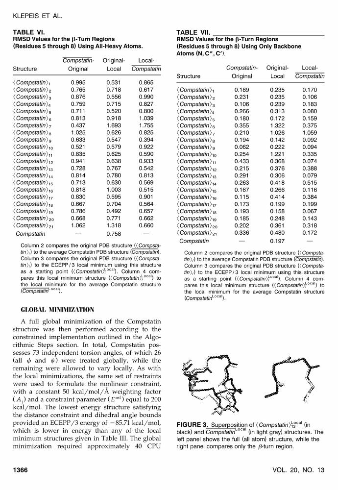
² :Local (FIGURE 3. Superposition of Compstatin in13Local) ( )black and Compstatin in light gray structures. The

( )left panel shows the full all atom structure, while theright panel compares only the b-turn region.

VOL. 20, NO. 131366


hours on a HP C160. As with the local minimiza-tions, the global minimum structure reached the200 kcalrmol bound on the violation energy con-

Ž .straint. The total distance violation D equaledVIO˚6.690 A, which is near the average distance viola-

tion from those local minimum structures given inTable III.

A number of RMSD calculations were per-formed to further quantify the structural differ-ences between the global minimum energy struc-ture and the other Compstatin structures. Theseresults are given in Tables VIII and IX. Table VIII

Ž .provides all-atom and backbone atom RMSD val-ues between the full local minimum energy struc-

Local LocalŽ² : .tures Compstatin and Compstatin andi

the global minimum energy structure. When com-² :Localparing backbone RMSDs, the Compstatin ,9

² :Local ² :Local ²Compstatin , Compstatin , and Compsta-21 19:Localtin structures offer the best correspondence17

with the global minimum energy structure. Thesestructures also correspond to four of the lowestenergy local minima as given in Table III. This

TABLE VIII.RMSD Values for Full Compstatin Structures.

Structure Heavy Atoms Backbone Atoms



Column 2 reports RMSD using all heavy atoms, while 3( a )accounts for only backbone atoms N, C , C9 . Both columns

(²compare the ECEPP / 3 local minimum structures Comp-L ocal L ocal: )statin and Compstatin to the global minimumi

( Global)Compstatin PDB structure Compstatin .

indicates that some of the lowest energy conform-ers exhibit similar backbone structural characteris-tics. However, it is interesting to note that the

² :Locallowest energy local minimum, Compstatin , is2

less similar to the global minimum energy struc-ture. Table IX provides RMSD values comparingonly the b-turn section of the Compstatin struc-ture. In this case, the lowest energy local minimado not necessarily provide the best correspondencewith the global minimum energy structure. Thisobservation, coupled with the relatively low RMSDvalues between all structures, indicates that theb-turn structure is a dominant characteristic for allconformers, including the global minimum energy

Žstructure. Plots for superpositioning backbone.atoms of the average local minimum energy struc-

Localture Compstatin and the global minimum en-ergy structure are given in Figure 4. The superpo-sitioning of these two structures results in char-acteristic RMSD values, as given in Tables VIIIand IX.

TABLE IX.RMSD Values for the b-Turn Regions( )Residues 5 through 8 .

Structure Heavy Atoms Backbone Atoms




(²compare the ECEPP / 3 local minimum structures Comp-L ocal L ocal: )statin and Compstatin to the global minimumi

( Global)Compstatin PDB structure Compstatin .


KLEPEIS ET AL.

( )FIGURE 4. Superposition of global minimum in blackLocal ( )and Compstatin in light gray structures. The left

( )panel shows the full backbone atom structure, whilethe right panel compares only the b-turn region.

COMPARISON WITH TAD: DYANA

A comparison to an independent method forsolving distance restraint problems was also madeto gauge the performance of the proposed aBBconstrained formulation. Specifically, a torsional

Žangle dynamics rather than a Cartesian coordinate. 5dynamics such as X-PLOR package was used.

The coupled simulated annealingrTAD protocolfrom DYANA was applied to a starting sample of1000 randomly generated structures. The same di-hedral angle constraints and 53 medium andlong-range distance constraints were considered;that is, no heuristic methods for reducing thevariable space were employed. In the case of un-specified symmetric hydrogens, a pseudoatom ap-proach, in which the restraint is based on a pseu-doatom central to the symmetric hydrogen atoms,was used. A subset consisting of the 20 conformersexhibiting the best target values were then used asstarting points for a second set of runs. Finally, a

Žset of five conformations with the smallest viola-.tions were used for further analysis. Because each

Ž .method DYANA vs. ECEPPr3 employed differ-ent structural definitions, based on fixed bondlengths and bond angles, a direct comparison wasnot sufficient. Instead, the DYANA generatedstructures were used as starting points for localminimizations using the local constrained formula-tion. In all cases, the violations reached the upperbound of 200 kcalrmol for E ref. The correspondingviolation values, including final local minimum

Ž .energy values E are given in Table X.ECEPPr3The results given in Table X indicate that al-

though the DYANA conformers satisfy the corre-sponding constraint, their energy values are signif-icantly higher than that of the global minimum

Ž .energy structure more than 70 kcalrmol . This

TABLE X.Local Minimization Results for the Best DYANA( )TAD -Generated Conformations.

E EVIO ECEPP/3

˚( ) ( ) ( )Local Minimum D A kcal / mol kcal / molVIO

DYANACompstatin 6.234 200.0 y11.9451DYANACompstatin 6.538 200.0 6.7822DYANACompstatin 6.163 200.0 y10.2083DYANACompstatin 5.476 200.0 y14.5164DYANACompstatin 6.927 200.0 5.0065

D refers to the total distance violation, E is the corre-VIO VIOsponding violation, and energy and E is the forceECEPP/ 3field energy at the local minima.

can be anticipated because the goal of the DYANAalgorithm is to minimize distance restraint viola-tions via penalty term optimization, while neglect-ing any detailed force field terms. In fact, an analy-sis of the structural characteristics indicate that thetype I b-turn does not appear along the Gln5]Gly 8

backbone in these structures. This is verified bythe data in Table XI, which gives the f and cdihedral angle values for the central b-turnresidues. The problem is evidenced by the Asp6

residue, which has f]c values in a forbiddenregion of the Ramachandran plot. It appears thatthis may be related to clustering of the side chainsin the DYANA predicted structures.

Including Intraresidue Restraints with DYANA

To further examine this deviation from the pre-Ž .vious results which define a type I b-turn the

DYANA protocol was also tested on the full set ofrestraints, including intraresidue distances. Thefive DYANA predicted structures exhibiting thelowest target function values were then subjected

TABLE XI.f and c Values for Central Residues

6 7( )Asp and Trp for the Anticipated b-Turn Region.

o o o o( ) ( ) ( ) ( )Local Minimum f c f c2 2 3 3

DYANACompstatin 166.9 y66.07 y80.00 y40.401DYANACompstatin 165.9 y65.55 y81.02 y33.992DYANACompstatin 180.0 y60.94 y81.76 y42.433DYANACompstatin 168.8 y50.32 y80.00 y42.224DYANACompstatin 165.4 y72.75 y97.79 y39.865

The subscripts refer to the second and third residues in theGln5 ]Gly8 sequence.

VOL. 20, NO. 131368


to local minimization using the constrained formu-lation. As before, only the 53 medium and long-range distance restraints were included during thelocal minimizations. As the results in Table XIIshow, the average energy has decreased for thisset of conformers. However, the structural analysisof the Gln5]Gly 8 region, given in Table XIII stillindicates that a type I b-turn is not preferred.

An additional comparison between the struc-Ž .tural characteristics of these DYANA local min-

ima and the global minimum was also performedusing RMSD calculations, as given in Tables XIVand XV. These values are consistently larger

LocalŽ .than those between the average Compstatinand local minimum solutions structuresŽ² :Local.Compstatin , and global minimum energyi

structure. The RMSD values not only indicate thatthere is significant structural difference over the

Ž .entire structure Table XIV , but also that theŽ .b-turn region Table XV is not a structural charac-

teristic of the DYANA local minima. This is evi-denced by the superpositioning of the lowest en-ergy DYANA structure and the global minimumenergy structure, given in Figure 5.

TABLE XII.Local Minimization Results for the Best DYANA( )TAD -Generated Conformations UsingAll Restraints.

E EVIO ECEPP/3

˚( ) ( ) ( )Local Minimum D A kcal / mol kcal / molVIO

DYANACompstatin 6.222 200.0 24.7141cDYANACompstatin 5.643 200.0 y31.2162cDYANACompstatin 6.527 200.0 y17.5693cDYANACompstatin 7.135 200.0 y27.11044DYANACompstatin 5.926 200.0 y14.6565c

D refers to the total distance violation, E is the corre-VIO VIOsponding violation, and energy and E is the forceECEPP/ 3field energy at the local minima.

TABLE XIII.f and c Values for Central Residues

6 7( )Asp and Trp for the Anticipated b-Turn Region.

o o o o( ) Ž . Ž . Ž .Local Minimum f c f c2 2 3 3

DYANACompstatin y180.0 y58.61 y80.00 y47.721cDYANACompstatin 177.5 y63.77 y82.74 y33.532cDYANACompstatin 180.0 y63.98 y82.18 y23.323cDYANACompstatin 163.0 y58.56 y109.2 y4.534cDYANACompstatin y180.0 y70.46 y92.40 y41.225c

The subscripts refer to the second and third residues in theGln5 ]Gly8 sequence.

TABLE XIV.RMSD Values for Full Compstatin Structures.

Local Minimum Heavy Atoms Backbone Atoms

DYANACompstatin 4.117 2.8121cDYANACompstatin 4.866 3.8932cDYANACompstatin 5.243 3.9433cDYANACompstatin 4.892 2.6544cDYANACompstatin 4.506 3.1805c


compare the DYANA local minimum structures( DYANA )Compstatin to the global minimum Compstatin PDBi

( Glob a l )structure Compstatin .

TABLE XV.RMSD Values for the b-Turn Regions( )Residues 5 through 8 .

Local Minimum Heavy Atoms Backbone Atoms

DYANACompstatin 1.163 0.6251cDYANACompstatin 1.473 0.7322cDYANACompstatin 1.607 0.7213cDYANACompstatin 1.327 0.7214cDYANACompstatin 1.277 0.7815c


compare the DYANA local minimum structures( DYANA )Compstatin to the global minimum Compstatin PDBi

( Glob a l )structure Compstatin .

Concluding Remarks

In this work a novel and completely generalmethod was outlined for solving the three-dimen-sional protein and nucleic acid structure predictionproblem using conformational restraints derivedfrom NMR data. In several ways, the method con-trasts strongly with typical techniques that rely on

( )FIGURE 5. Superposition of global minimum in blackDYANA ( )and Compstatin in gray structures. The left panel1c

( )shows the full backbone atom structure, while the rightpanel compares only the b-turn region.


KLEPEIS ET AL.

the optimization of penalty-type target functionusing simulated annealing and molecular dynam-

Ž .ics plus local minimization protocols.One difference involves a novel reformulation

of the structure prediction problem. A commoncharacteristic of most current methods is their de-pendence on a penalty-type, unconstrained prob-lem formulation, in which the objective is to mini-mize the sum of violation energies. In this work,the problem is formulated using nonlinear con-straints, which can be individually enumerated forall or subsets of the distance restraints. In addition,the simplified potential function used by manytechniques is replaced by a full-atom force field,which aids in defining the correct conformationaldetails.

Finally, the solution technique represents an-other enhancement over existing methods. Ratherthan rely on stochastic methods for finding low-energy minima, this work utilizes a deterministicmethod, which theoretically guarantees that theglobal solution will be located. This branch andbound technique, based on the aBB algorithm, hasalready been successfully applied to the identifica-tion of global minimum energy structures of pep-tides modeled by full-atom force fields.

The application of this technique to the Comp-statin structure prediction problem emphasizes themerits of the approach. The globally predictedstructure agrees with previous results based onX-PLOR4 when comparing structural characteris-tics, such as the formation of a type I b-turn.However, the overall structure exhibits an im-proved energy, which indicates better definition ofstructural details. In contrast, results obtained fromTAD fail to identify a type I b-turn. This is mostlikely attributable to the simplistic form of energymodeling and the difficulties in searching the con-formational space.

Acknowledgments

CAF gratefully acknowledges financial supportfrom the National Science Foundation, Air ForceOffice of Scientific Research, and the National In-

Ž .stitutes of Health R01 GM52032 .

References

1. Braun, W.; Go, N. J Mol Biol 1985, 186, 611.2. Guntert, P.; Braun, W.; Wuthrich, K. J Mol Biol 1991, 217,¨ ¨

517.

3. Guntert, P.; Wuthrich, K. J Biomol NMR 1991, 1, 446.¨ ¨4. Brunger, A. T. X-PLOR User Guide; Yale University Press:¨

New Haven, 1992.5. Guntert, P.; Mumenthaler, C.; Wuthrich, K. J Mol Biol 1997,¨ ¨

273, 283.6. Rice, L. M.; Brunger, A. T. Proteins 1994, 19, 277.¨7. Brunger, A. T.; Adams, P. D.; Rice, L. M. Structure 1997, 5,¨

325.8. Nilges, M. Curr Opin Struct Biol 1996, 6, 617.9. Torda, A. E.; van Gunsteren, W. F. In Reviews in Computa-

tional Chemistry; Lipkowitz, K. B.; Boyd, D. B. Eds.; VCHPublishers: Weinheim, 1992, p. 143, vol. 3.

10. Adjiman, C. S.; Androulakis, I. P.; Maranas, C. D.; Floudas,C. A. Comput Chem Eng 1996, 20, S419.

11. Adjiman, C. S.; Androulakis, I. P.; Floudas, C. A. ComputChem Eng 1997, 21, S445.

12. Adjiman, C. S.; Androulakis, I. P.; Floudas, C. A. ComputChem Eng 1998, 22, 1159.

13. Adjiman, C. S.; Dallwig, S.; Floudas, C. A.; Neumaier, A.Comput Chem Eng 1998, 22, 1137.

14. Androulakis, I. P.; Maranas, C. D.; Floudas, C. A. J GlobOpt 1995, 7, 337.

15. Morikis, D.; Assa]Munt, N.; Sahu, A.; Lambris, J. D. Pro-tein Sci 1998, 7, 619.

16. Nementhy, G.; Gibson, K. D.; Palmer, K. A. Yoon, C. N.;´Paterlini, G.; Zagari, A.; Rumsey, S.; Scheraga, H. A. J PhysChem 1992, 96, 6472.

17. Floudas, C. A.; Klepeis, J. L.; Pardalos, P. M. In DIMACSSeries in Discrete Mathematics and Theoretical ComputerScience, American Mathematical Society: Providence, RI,1999, p. 141, vol. 47.

18. Floudas, C. A. In Large Scale Optimization with Applica-tions, Part II: Optimal Design and Control, Biegler, L. T.;Coleman, T. F.; Conn, A. R.; Santosa, F. N., Eds. IMAVolumes in Mathematics and its Applications; Springer-Verlag: Berlin, 1997, p. 129, vol. 93.

19. Maranas, C. D.; Floudas, C. A. J Chem Phys 1992, 97, 7667.20. Maranas, C. D.; Floudas, C. A. Ann Oper Res 1993, 42, 85.21. Maranas, C. D.; Floudas, C. A. J Chem Phys 1994, 100, 1247.22. Maranas, C. D.; Floudas, C. A. J Glob Opt 1994, 4, 135.23. Androulakis, I. P.; Maranas, C. D.; Floudas, C. A. J Glob

Opt 1997, 11, 1.24. Maranas, C. D.; Androulakis, I. P.; Floudas, C. A. In DI-

MACS Series in Discrete Mathematics and TheoreticalComputer Science; American Mathematical Society: Provi-dence, RI, 1996, p. 133, vol. 23.

25. Klepeis, J. L.; Androulakis, I. P.; Ierapetritou, M. G.; Floudas,C. A. Comput Chem Eng 1998, 22, 765.

26. Klepeis, J. L.; Floudas, C. A. J Comput Chem, 1999, 20, 636.27. Adjiman, C. S.; Floudas, C. A. J Glob Opt 1996, 9, 23.28. Scheraga, H. A. PACK: Programs for Packing Polypeptide

Chains, 1996, online documentation.29. Gill, P. E.; Murray, W.; Saunders, M. A.; Wright, M. H.

NPSOL 4.0 User’s Guide; Systems Optimization Labora-tory, Dept. of Operations Research, Stanford University:Stanford, CA, 1986.

Ž30. Klepeis, J. L.; Floudas, C. A. 1999, submitted for publica-.tion .

31. Sahu, A.; Kay, B. K.; Lambris, J. D. J Immunol 1996, 157,884.

VOL. 20, NO. 131370

Documents

Predicting peptide structures using NMR data and deterministic global optimization