Embed Size (px)
Citation preview
PREDICTING HPGR PERFORMANCE AND UNDERSTANDING ROCK PARTICLE
BEHAVIOR THROUGH DEM MODELLING
by
Amit Kumar
B.Tech. (Mineral Engineering), Indian School of Mines, 2011
M.Tech. (Mineral Resource Management), Indian School of Mines, 2011
A THESIS SUBMITTED IN PARTIAL FULFILLMENT OF THE REQUIREMENTS FOR
THE DEGREE OF
MASTER OF APPLIED SCIENCE
in
THE FACULTY OF GRADUATE AND POSTDOCTORAL STUDIES
(Mining Engineering)
THE UNIVERSITY OF BRITISH COLUMBIA
(Vancouver)
April 2014
© Amit Kumar, 2014

ii
Abstract
High pressure grinding rolls (HPGR) are becoming an increasingly popular energy efficient
solution for comminution of hard rock ores. A significant barrier to the increased adaptation of
HPGRs is the current requirement for large amounts of sample for pilot testing.
The primary objective of the research was to develop a DEM based computer model for an
HPGR to analyze the particle behavior in the unit and to predict its sizing information. EDEM, a
DEM based software, was used to model the pilot scale HPGR unit and single particle
compression test was used to evaluate the particle breakage and then used as an input parameter
for the simulations. The results obtained from the simulation were then validated with the results
from the pilot scale tests.
Results obtained from the simulation suggested that a DEM-based model can be used to identify
the pressure/force distribution profile for an HPGR roll surface that can then be used to design
the appropriate piston geometry to match the HPGR pressure profile. Also, the developed HPGR
model was used to estimate the critical sizing information for certain samples and machine
operating conditions. The model generated similar trends as the pilot scale test with a lower
magnitude of m-dot and specific energy consumption primarily due to the absence of a packed
particle bed.
The HPGR model, combined with powerful computers and larger sample masses for simulation,
can be used as a procedure to size and select an industrial HPGR unit and to analyze the
equipment behavior under various operating conditions and feed characteristics.

iii
Preface
This project work is a part of the UBC HPGR research program that took place at the University
of British Columbia, and was supported by the Canadian Mining Industry Research Organization
(CAMIRO). The objective was to develop an HPGR model to evaluate its working behavior and
performance under different operating conditions.
Under the supervision of Dr. Bern Klein, professor at the Norman B. Keevil Institute of Mining
Engineering at the University of British Columbia, I was responsible for developing the test
program, conducting the test work and interpreting the results.
Zorigkhuu Davaanyam and Stefan Nadolski assisted with the HPGR and piston-die tests and in
interpreting the data. Data provided in Appendix B is based on the HPGR pilot test results
provided by Zorigkhuu Davaanyam.
iv
Table of contents
Abstract .......................................................................................................................................... ii
Preface ........................................................................................................................................... iii
Table of contents .......................................................................................................................... iv
List of tables................................................................................................................................ viii
List of figures ................................................................................................................................ ix
List of symbols ............................................................................................................................. xii
List of abbreviations .................................................................................................................. xiv
Acknowledgements ......................................................................................................................xv
Chapter 1: Introduction ................................................................................................................1
1.1 Background ..................................................................................................................... 1
1.2 Thesis objectives ............................................................................................................. 3
1.3 Thesis outline .................................................................................................................. 4
Chapter 2: Literature review ........................................................................................................5
2.1 Introduction ..................................................................................................................... 5
2.2 High pressure grinding rolls ............................................................................................ 5
2.2.1 HPGR history and adaptation ..................................................................................... 6
2.2.2 HPGR configuration and fundamentals ...................................................................... 8
2.2.3 HPGR critical sizing parameters ............................................................................... 10
2.2.4 HPGR benefits .......................................................................................................... 12
2.2.5 Disadvantages of HPGR ........................................................................................... 14

v
2.2.6 HPGR sizing ............................................................................................................. 14
2.2.7 Effects of variable parameters .................................................................................. 15
2.2.8 Pressure distribution on HPGR roll .......................................................................... 19
2.3 Piston-die test ................................................................................................................ 22
2.4 Computer modelling and simulation ............................................................................. 23
2.4.1 Introduction ............................................................................................................... 23
2.4.2 Discrete element method modelling ......................................................................... 24
2.4.3 DEM basics ............................................................................................................... 26
2.4.4 DEM modelling challenges....................................................................................... 28
2.4.5 Particle breakage modelling ...................................................................................... 28
Chapter 3: EDEM software and model set-up ..........................................................................32
3.1 EDEM software ............................................................................................................ 33
3.2 Limitations of EDEM ................................................................................................... 35
3.3 Model set-up ................................................................................................................. 38
3.3.1 Particle-particle interaction model ............................................................................ 38
3.3.2 Particle-geometry contact model .............................................................................. 43
3.3.3 Particle body force (breakage model) ....................................................................... 43
3.3.4 Material properties and interactions.......................................................................... 46
3.3.5 HPGR geometry ........................................................................................................ 47
3.3.6 Motion of geometries ................................................................................................ 49
3.3.7 Base particle definition ............................................................................................. 51

vi
3.3.8 Defining the domain ................................................................................................. 53
3.3.9 Particle factory .......................................................................................................... 54
3.3.10 Particle breakage factory ....................................................................................... 56
3.3.11 Timestep ................................................................................................................ 57
3.3.12 Simulation time ..................................................................................................... 58
Chapter 4: Experimental procedures.........................................................................................59
4.1 Methodology ................................................................................................................. 59
4.2 Sample description ........................................................................................................ 60
4.3 Pilot scale HPGR test .................................................................................................... 61
4.4 Single particle compression test.................................................................................... 63
Chapter 5: Results and discussions ............................................................................................67
5.1 Force and pressure distribution modelling .................................................................... 67
5.1.1 HPGR force distribution ........................................................................................... 67
5.1.2 Pressure distribution and piston geometry ................................................................ 73
5.1.3 Pressure distribution and particle size ....................................................................... 78
5.2 HPGR tests and simulation analysis ............................................................................. 87
5.2.1 HPGR pilot testing results ........................................................................................ 87
5.2.2 Single particle compression testing results ............................................................... 91
5.2.3 DEM model results ................................................................................................... 97
5.2.4 Model vs. pilot scale results .................................................................................... 103
Chapter 6: Conclusions and recommendations ......................................................................111

vii
6.1 Major research findings .............................................................................................. 111
6.2 Recommendations for future testwork ........................................................................ 114
References ...................................................................................................................................115
Appendices ..................................................................................................................................125
Appendix A – HPGR experiment data.................................................................................... 125
Appendix B - Single particle compression tests ..................................................................... 137
B.1 Iron ore ......................................................................................................................... 137
B.2 Copper ore .................................................................................................................... 142

viii
List of tables
Table 2-1: Actual lifetime hours achieved by HPGR roll surfaces .............................................. 10
Table 3-1: Material properties ...................................................................................................... 46
Table 3-2: Particle and roll surface interactions ........................................................................... 47
Table 3-3: Particle sizes for simulation for iron ore ..................................................................... 52
Table 3-4: Particle sizes for simulation for copper ore ................................................................. 53
Table 3-5: Number of particles for simulation ............................................................................. 55
Table 4-1: Technical specifications of the pilot HPGR unit ......................................................... 62
Table 4-2: Single particle compression test samples .................................................................... 65
Table 5-1: HPGR pilot scale test results summary ....................................................................... 88
Table 5-2: HPGR modelling results summary ............................................................................ 100
Table 5-3: Throughput and m-dot (pilot scale vs. modelled results) .......................................... 106
Table 5-4: P80 and P50 for iron ore (pilot scale vs. modelled results) ......................................... 108

ix
List of figures
Figure 2-1: HPGR growth in the mining industry .......................................................................... 7
Figure 2-2: HPGR configuration .................................................................................................... 9
Figure 2-3: Effect of roll speed on specific energy consumption and specific throughput .......... 17
Figure 2-4: Effect of roll speed on specific energy consumption ................................................. 18
Figure 2-5: Compression and nip angle in an HPGR ................................................................... 19
Figure 2-6: Pressure distribution with compression angle ............................................................ 20
Figure 2-7: Pressure profile across roll width ............................................................................... 21
Figure 2-8: Pressure distribution across roll width ....................................................................... 21
Figure 2-9: Particle breakage model ............................................................................................. 30
Figure 3-1: EDEM analysis loop .................................................................................................. 33
Figure 3-2: HPGR simulation results from 100mm feed to 35mm product size .......................... 36
Figure 3-3: Shear modulus vs. simulation run time ...................................................................... 37
Figure 3-4: Schematic diagram for Hertz-Mindlin contact model................................................ 39
Figure 3-5: Particle replacement with two particles ..................................................................... 44
Figure 3-6: Particle replacement with cluster ............................................................................... 45
Figure 3-7: HPGR geometry from EDEM .................................................................................... 48
Figure 3-8: Forces on the floating roll .......................................................................................... 50
Figure 4-1: Experimental program description ............................................................................. 60
Figure 4-2: Pilot HPGR installed at UBC Mining Engineering ................................................... 61
Figure 4-3: MTS hydraulic press installed at UBC Mining Engineering ..................................... 64

x
Figure 5-1: Compressive force on the particles at different pressing forces ................................ 68
Figure 5-2: Total compressive force on particles across roll width .............................................. 70
Figure 5-3: Worn out HPGR roll at Cerro Verde mine, Peru ....................................................... 71
Figure 5-4: Average compressive force on each particle across roll width .................................. 72
Figure 5-5: Average pressure on roll surface across the roll width .............................................. 72
Figure 5-6: Piston geometries ....................................................................................................... 74
Figure 5-7: Floor pressure distribution with piston-1 ................................................................... 75
Figure 5-8: Floor pressure distribution with piston-2 ................................................................... 76
Figure 5-9: Floor pressure distribution with piston-3 ................................................................... 76
Figure 5-10: Floor pressure distribution with piston-4 ................................................................. 77
Figure 5-11: Die floor pressure at 1 second (-12.5+11.2mm) ...................................................... 79
Figure 5-12: Die floor pressure at 1 second (-6.7+5.6mm) .......................................................... 80
Figure 5-13: Die floor pressure at 1 second (-2.8+2.0mm) .......................................................... 80
Figure 5-14: Die floor pressure at 4 seconds (-12.5+11.2mm) ..................................................... 81
Figure 5-15: Die floor pressure at 4 seconds (-6.7+5.6mm) ......................................................... 81
Figure 5-16: Die floor pressure at 4 seconds (-2.8+2.0mm) ......................................................... 82
Figure 5-17: Die floor pressure at 8 seconds (-12.5+11.2mm) ..................................................... 82
Figure 5-18: Die floor pressure at 8 seconds (-6.7+5.6mm) ......................................................... 83
Figure 5-19: Die floor pressure at 8 seconds (-2.8+2.0mm) ......................................................... 83
Figure 5-20: Die floor pressure at 12 seconds (-12.5+11.2mm) ................................................... 84
Figure 5-21: Die floor pressure at 12 seconds (-6.7+5.6mm) ....................................................... 85

xi
Figure 5-22: Die floor pressure at 12 seconds (-2.8+2.0mm) ....................................................... 85
Figure 5-23: Effect of specific pressing force on net specific energy consumption ..................... 89
Figure 5-24: Effect of specific pressing force on specific throughput constant ........................... 90
Figure 5-25: Effect of roll speed on net specific energy consumption and specific throughput
constant ......................................................................................................................................... 91
Figure 5-26: Single particle compression test result (iron ore)..................................................... 92
Figure 5-27: Single particle compression test result (copper ore) ................................................ 92
Figure 5-28: Force per unit mass vs. particle size ........................................................................ 94
Figure 5-29: Threshold energy vs. particle size for iron ore......................................................... 95
Figure 5-30: Threshold energy vs. particle size for copper ore .................................................... 96
Figure 5-31: Operating gap vs. time at different pressing force (iron ore) ................................... 98
Figure 5-32: Operating gap vs. time at different roll speed (iron ore) .......................................... 98
Figure 5-33: Operating gap vs. time at different pressing force (copper ore) .............................. 99
Figure 5-34: Simulated effect of specific pressing force on net specific energy consumption .. 101
Figure 5-35: Simulated effect of specific pressing force on specific throughput constant ......... 102
Figure 5-36: Simulated effect of roll speed on net specific energy consumption and specific
throughput constant for iron ore ................................................................................................. 102
Figure 5-37: Operating gap (pilot scale vs. modelled results) .................................................... 104
Figure 5-38: Product size distribution for iron ore (pilot scale vs. modelled results) ................ 107
Figure 5-39: Energy consumption (pilot scale vs. modelled results).......................................... 109
Figure 5-40: Energy consumption for both ore types (pilot scale vs. modelled results) ............ 110
Figure 6-1: Approach for small scale test procedure .................................................................. 113

xii
List of symbols
Symbol Description
Fsp Specific pressing force
D Roll diameter
W Roll width
Esp Net specific energy consumption
Pt Total motor power draw
Pi Idle motor power draw
Q Throughput
m-dot Specific throughput constant
V Roll peripheral speed
vi Transitional velocity
ωi Angular velocity
Ii Moment of inertia
R Particle radius
Fn Normal force
Ft Tangential force
E*
Young’s modulus
m Mass of particles
v Poisson’s ration
R* Equivalent radius

xiii
m* Equivalent mass
E Coefficient of restitution
Sn Normal stiffness
vnrel
Relative normal velocity
vtrel
Relative tangential velocity
G*
Equivalent shear modulus
St Tangential stiffness
µr Coefficient of rolling friction
µs Coefficient of static friction
τ Torque
δn Normal overlap
δt Tangential overlap
X Position on x-axis
Y Position on y-axis
Z Position on z-axis
F80 80% passing feed
P80 80% passing product
F50 50% passing feed
P50 50% passing product

xiv
List of abbreviations
Abbreviation Description
ROM Run of mine
AG Autogenous grinding
SAG Semi-autogenous grinding
HPGR High pressure grinding roll
SABC Semi-autogenous/ball mill/crushing
DEM Discrete element method
RPM Revolutions per minute
SPT Static pressure test
API Advanced programming interface
PSD Particle size distribution

xv
Acknowledgements
I would like to express my appreciation to all those on my supervisory committee, and also to
provide a special thank you to my supervisor Dr. Bern Klein, for his supervision, guidance and
support throughout this research project. I would like to express my gratitude for the support of
all the sponsors involved in providing the equipment and funds necessary for this study.
I would also like to convey my gratefulness to Koeppern Machinery Australia for providing the
pilot HPGR results that were used for validation. I would like to acknowledge Senthil
Arumugam, Ammar Khaliq, Mark Cook and Stephen Cole for providing me assistance with
training and consultation with respect to software usage and coding.
The assistance of Zorigkhuu Davaanyam, Stefan Nadolski, Chengtie Wang and Yu Hou in
performing the HPGR and piston-die tests, and their constant support and guidance are also
deeply acknowledged.
I would like to appreciate the emotional support and love received from my friends most
particularly Jaishankar Iyer, Tugs Tsedenbaljir, Enkhbold Tsagaabkhuu, Solongo Bumtseren,
Dulguun Dukunuu and Linlin Zhang who helped make my stay enjoyable and pleasant.
Finally, I would like to thank my parents and siblings for their love and constant support.

1
CHAPTER 1: INTRODUCTION
1.1 Background
Comminution is the process of reducing the size of run of mine (ROM) ore, and is accomplished
through the application of mechanical forces in order to separate the valuable minerals from
unwanted gangue minerals. It begins with the blasting of rocks in the mine and is then further
achieved through crushing and grinding. The mechanism of size reduction can be classified as
impact/compression and abrasion/chipping (Drozdiak, 2013).
Crushers such as jaw, gyratory or cone crushers and grinders such as AG, SAG or ball mills are
the most commonly used comminution equipment in processing plants. Pease (2007) has
suggested that comminution consumes 3% of the total energy around the globe. Approximately
50-80% of the total energy consumption in a mineral processing plant is utilized by comminution
equipment (Abouzeid & Fuerstenau, 2009; Haque, 1999; Wang, 2013), rendering comminution
as an energy intensive process. The efficiency of grinding equipment can be as low as 1%
(Haque, 1999), which makes comminution highly energy inefficient. A decrease in the metal
grade of ROM ore and increased plant throughput during last decades has forced researchers to
look into more energy-efficient comminution processes.
The High Pressure Grinding Roll (HPGR) is one of the more energy efficient comminution units
for hard rock ores. Studies have suggested that HPGR-based circuits are 10-25% more energy
efficient than conventional SABC circuits (Von Michaelis, 2009; Wang 2013). A significant
barrier to the increased adaption of HPGRs is the current requirement for a high quantity of

2
sample for pilot testing. A typical HPGR test for sizing and selection requires approximately 1-5
tonnes of samples. Various studies using a piston and die arrangement have been conducted to
analyze the performance of lab scale HPGR and thus simulate the behavior of industrial scale
units. The piston-die tests have not however, been accepted worldwide for sizing HPGR units.
In order to develop a small-scale procedure for HPGR assessment, the motion of feed particles
and the distribution of roll forces and particle interactions need to be understood. The
understanding of particle movement and force distribution in a piston-die arrangement would
also assist in the development of small-scale testing and their accompanying procedures.
Modelling methods, such as the Discrete Element Method (DEM), provide a means through
which to understand these behaviors. DEM-based software packages have been used successfully
in the design and optimization of comminution equipment such as gyratory crushers, rod and ball
mills, SAG mills and stirred mills.
In this research, a working model for the HPGR has been developed using EDEM (a DEM based
software) which is validated against the pilot-scale test results using two different sample types.
At the same time, the pressure distributions in a piston die arrangement have also been analyzed
using different piston arrangements to simulate the behavior of the pressure distribution in an
HPGR unit across the roll width.

3
1.2 Thesis objectives
The primary objective of this research was to develop a working model of an HPGR which could
then be used to predict the sizing information for an HPGR unit especially with regard to the
energy consumption and throughput. In order to achieve the primary objective of the research,
the following intermediate objectives were targeted:
Developing a computer model for HPGR using Discrete Element Method to better
understand the rock particle behavior and to predict HPGR sizing information.
Gaining an understanding of the HPGR configuration and developing an HPGR geometry
similar to that of the pilot scale unit available at the NBK Institute of Mining Engineering.
Studying single particle compression test, developing a procedure to analyze threshold force
for rock breakage for a given ore and using it as an input parameter for the HPGR computer
model to be developed.
Creating the computer model for HPGR that simulates the pilot scale unit at various
operating conditions.
Analyzing the force/pressure distribution profile on HPGR rolls and simulating the pressure
distribution in a piston-die arrangement using different piston geometries to compare the two
distributions.
Comparing the HPGR behavior from available pilot scale results and modelled outputs at
different operating conditions in order to validate the DEM model performance.

4
1.3 Thesis outline
Chapter 2 provides a literature review on HPGR and its different aspects as they relate to sizing
and selection. This chapter also discusses important and relevant terminologies and includes a
preview of the piston-die arrangement used for HPGR scale-up. This section also covers the
basic of DEM modelling and its application for the optimization of comminution equipment.
Chapter 3 discusses EDEM software and provides the details needed for model development
setup.
Chapter 4 describes the experimental procedure followed for HPGR tests and lab scale single
particle breakage tests.
Results and discussions regarding lab tests, pilot tests and computer model results are presented
in Chapter 5 along with the model validation.
This thesis is concluded in Chapter 6 with the presentation of the study’s main conclusions and
recommendations for future work.

5
CHAPTER 2: LITERATURE REVIEW
2.1 Introduction
Run of mine (ROM) ore contains valuable minerals locked within the unwanted gangue
materials. The rock size needs to be reduced in order to liberate the valuable from the gangues.
Comminution involves the process of reducing the size of ROM ore to prepare it for subsequent
processing.
Crushing equipment such as jaw crushers, gyratory crushers and cone crushers followed by rod
mills and ball mills made up the conventional flow-sheet designs used until 1950’s. With a
gradual increase in plant throughput, it became necessary to develop new equipment to handle
the higher tonnage. Autogenous (AG) mills and semi-autogenous (SAG) mills, and subsequently
followed by ball mills gained popularity due to their higher proficiencies in handling capacity.
The grinding inefficiencies of both AG and SAG mills were the prime factors prompting
researchers to continue research into more energy-efficient comminution equipment. HPGRs are
one of the most energy-efficient types of equipment that have gained favor in hard rock mining
over the past decade.
2.2 High pressure grinding rolls
In order to develop the computer model for an HPGR, its fundamentals, configuration and
associated parameters need to be studied and analyzed. This section provides detailed

6
information regarding the history and adaptation of HPGR in hard rock mining, its geometry
description, working fundamentals, and parameters affecting its adaptation and performance.
2.2.1 HPGR history and adaptation
High pressure grinding rolls are a relatively new technology in the hard rock mining industry.
They are derived from the briquetting technique which uses high pressure double roll compactors
to press fine coal into solid lumps (Lynch & Rowland, 2005).
Schoenert (1979) has shown that the process of compressing particles between two plates is the
most energy-efficient method for rock breakage. HPGR was first introduced in the cement
industry in 1985 to grind clinkers. Aydoğan et al. (2006) used various HPGR circuit options to
show that closed circuit HPGR applications provide substantial energy savings in the cement
industry. By 2000, HPGR was used in many cement plants, and it was reported to provide up to
50% energy savings when compared to conventional circuits (Casteel, 2005).
After the adaptation in the cement industry, HPGR became widespread in the diamond industry
for secondary crushing and re-crushing. According to Daniel (2010), the liberation of high value
diamonds through the use of HPGR was the reason for the speed of its adaptation. Due to the
packed bed of particles and the relatively high pressure the system employed, minimal damage
was caused to the diamonds while the surrounding rocks were successfully broken. Premier
Diamond mine in South Africa installed the first HPGR in the diamond industry in 1987-88
(Casteel, 2005).

7
Following its adaptation in the diamond industry, HPGR was then embraced by the iron industry
to grind iron ore as a preparation for pelletization (Casteel, 2005). The adaptation of HPGR for
hard rock ore processing began in 1995 with an 18 month trial at Cyprus Sierrita copper mine in
Arizona, United States (Morley, 2010). According to Morley (2010), the overall machine
utilization was around 60%. This relatively low percentage was due to the difficulties and
experimentation with roll wear surfaces. Similar problems had also been experienced in the past
at Argyle diamond mine in Western Australia. Downtime due to liner wear and the reduced
availability of HPGR hindered its adaptation in hard rock mining. It took almost 10 years to
improve the HPGR technology to a level acceptable for its preparation for its first commercial
installation at Cerro Verde, Peru in 2006 (Casteel, 2005).
Figure 2-1 shows the number of installations of HPGR units in the mining industry over the last
20 years.
Figure 2-1: HPGR growth in the mining industry (Burchardt et al., 2011)

8
Burchardt et al. (2011) have noticed that HPGRs have been installed in various new plants
including Cerro Verde (Peru), Boddington (Western Australia), Mogalakwena (South Africa) to
function in tertiary crushing applications whereas at the PTFI Grasberg mine (Indonesia) HPGRs
have been proven successful for quaternary crushing applications. In October 2009, HPGR was
commissioned for Goldfields Tarkwa mine (Ghana) heap leach operations (Burchardt et al.,
2011).
2.2.2 HPGR configuration and fundamentals
A typical HPGR unit consists of two counter rotating rolls mounted in a frame. As shown in
Figure 2-2, one roll is fixed in the horizontal position whereas the opposite roll, referred as a
floating roll is able to move freely in the horizontal position according to the forces of the
particle bed and the hydraulic forces. The particle bed is created between the two rolls by gravity
choke feeding and compression is achieved through the application of a high pressure by the
hydraulics. Inter-particle compression breakage is responsible for the size reduction. Most
vendors have similar machine arrangements though with differences in roll width and diameter.

9
Figure 2-2: HPGR configuration (KHD Humboldt Wedag, 2011)
In the past, the major drawback of the system was the roll wear, which affected the availability
of HPGRs. Different vendors have different wear lining profiles such as Hexadur®, which was
developed by Koeppern Machinery (Germany). The autogenous layer formed during the
operations helps improve the life of HPGR rolls by providing a shield from the moving particle
bed. As seen in Table 2-1, KHD Humboldt Wedag (2011) has listed the linear lifetime hours
actually achieved in an HPGR.

10
Table 2-1: Actual lifetime hours achieved by HPGR roll surfaces (KHD Humboldt Wedag, 2011)
Type of Operation Operating hours (hrs)
Iron ore (pellet) 14000-36000
Iron ore (coarse) 6000-17000
Gold ore (coarse) 4000-6000
Kimberlite Rock (coarse) 4000-7000
Phosphate ore (coarse) 6000-12000
2.2.3 HPGR critical sizing parameters
To understand HPGR operations, several parameters and terminologies which are specific to
HPGR need to be clarified. These parameters are critical for pilot scale testing as well as for the
sizing of an industrial scale HPGR.
Operating gap
The operating gap is defined as the smallest distance between the fixed roll and the floating roll
during HPGR tests. The operating gap fluctuates depending upon the ore characteristics and
machine operating conditions.

11
Specific pressing force
Specific pressing force is the total force per unit of the projection area of the roll due to the
external forces exerted by the hydraulic cylinders as shown in Equation 2-1. This parameter
controls the energy consumption, operating gap and product size distribution rendering it as the
most critical parameter.
Equation 2-1
Where, Fsp is the specific pressing force (N/mm2), Ft is the total force exerted by the hydraulic
cylinders (N), D is roll diameter (mm) and W is the roll width (mm).
Net Specific Energy Consumption
Net specific energy consumption is the net power drawn from the motor per unit ton of ore
processed as shown in Equation 2-2. This parameter is used to size the motor for industrial scale
HPGRs.
Equation 2-2
Where, Esp is the net specific energy consumption (kWh/t), Pt is total motor power draw (kW), Pi
is idle motor power draw (kW) and Q is throughput (tph).

12
Specific throughput constant (m-dot)
The specific throughput constant, for a given material, is the throughput rate for an HPGR with
1m roll diameter, 1m roll width and 1m/s peripheral speed as shown in Equation 2-3. Based on
the m-dot information, the sizing for roll dimensions is performed on an industrial scale.
Equation 2-3
Where, m-dot is the specific throughput constant (ts/hm3), Q is throughput (tph), D is roll
diameter (m), W is the roll width (m) and V is the roll peripheral speed (m/s).
2.2.4 HPGR benefits
The increased adaption of an HPGR based circuits is due to its potential advantages over
conventional comminution circuits such as:
Energy Savings
Wang (2013) showed that HPGR-ball mill circuits provide 23-30% energy savings over the
AG/SAG mill-ball mill circuit. Several studies have found that HPGR-based circuits provide
significantly higher energy savings over conventional comminution circuits (Drozdiak, 2011;
Rosario & Hall, 2010; Schönert, 1988; Valery & Jankovic, 2004).

13
Bond ball mill work index
Wang (2013) has shown that an approximately 10-15% drop in the bond ball mill work index can
be achieved by using HPGR to produce ball mill feed. This drop can be used to increase the
throughput for the ball mill. Valery & Jankovic (2004) also listed that an increase in the specific
pressing force reduces the bond ball mill work index.
Micro-cracking and liberation
Compression breakage in the HPGR generates micro-cracks in the obtained product which help
in the downstream processes such as floatation and leaching (Morley, 2010; Von Michaelis,
2009). When compared to conventional technologies, HPGR produces more micro-factures and
produce better liberation for copper and gold ores (Esna-Ashari & Kellerwessel, 1988). Dunne
(1996) has suggested that micro-fractures improve the floatation recovery for coarse sized
fractions and leach extraction. McNab (2006) suggested that the degree of liberation depend on
the specific pressing force.
Savings in media cost
HPGR does not use any grinding media such as steel balls as in SAG mills, thus reducing the
operating costs for the HPGR. Due to enhanced life of the liner, the machine’s availability rises.
Furthermore, it also shows less sensitivity to the variability in ore hardness, thus helping to
provide a constant throughput.

14
2.2.5 Disadvantages of HPGR
In addition to its potential advantages over conventional comminution circuits, HPGR-based
circuits also have some disadvantages.
A typical HPGR circuit has a higher capital cost when compared to a conventional crushing
flow-sheet due to the need of extra screening and conveying equipment for feed preparation.
Cerro Verde, an HPGR operation in Peru, uses a secondary crusher in reverse closed circuit of a
vibratory screen for HPGR feed preparation followed by an HPGR in closed circuit of a screen,
which increases the capital cost by approximately 23% over that of an SAG circuit (Vanderbeek
et al., 2006; Wang, 2013).
Morley (2010) has also suggested that the higher moisture content in the feed reduces the HPGR
throughput and decreases the liner life as it prevents autogenous layer formation. Highly abrasive
ore also increases the linear wear rate and reduces the life of the liner.
2.2.6 HPGR sizing
Even with the advantage of energy savings and lower operating costs, the adaptation of HPGR
has been slow. The main reason for this has been the absence of a small lab-scale tests and
procedure for the sizing and selection of HPGR units.
A typical HPGR pilot scale test requires around 250-300kgs of sample, depending on the ore.
These tests provide information on specific energy consumption which is then used to size the
15
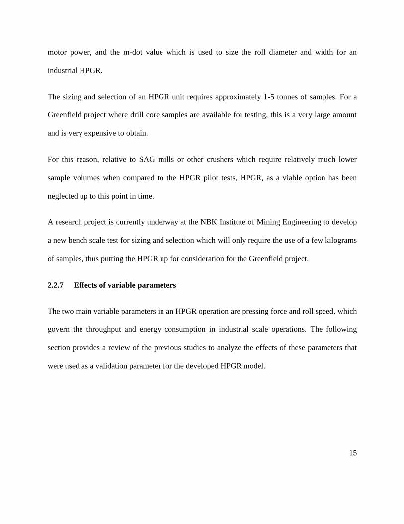
motor power, and the m-dot value which is used to size the roll diameter and width for an
industrial HPGR.
The sizing and selection of an HPGR unit requires approximately 1-5 tonnes of samples. For a
Greenfield project where drill core samples are available for testing, this is a very large amount
and is very expensive to obtain.
For this reason, relative to SAG mills or other crushers which require relatively much lower
sample volumes when compared to the HPGR pilot tests, HPGR, as a viable option has been
neglected up to this point in time.
A research project is currently underway at the NBK Institute of Mining Engineering to develop
a new bench scale test for sizing and selection which will only require the use of a few kilograms
of samples, thus putting the HPGR up for consideration for the Greenfield project.
2.2.7 Effects of variable parameters
The two main variable parameters in an HPGR operation are pressing force and roll speed, which
govern the throughput and energy consumption in industrial scale operations. The following
section provides a review of the previous studies to analyze the effects of these parameters that
were used as a validation parameter for the developed HPGR model.

16
Pressure
The specific pressing force applied by the piston on the floating roll governs the operating gap.
Increasing the pressing force decreases the operating gap and thus generates finer product size
distribution. At the same time, an increase in the force causes an increase in the torque which
eventually increases the total power draw from the motor.
Dundar et al. (2011) have shown that an increase in pressure decreases the operating gap
significantly, thus resulting in a drop in the throughput and it also increases the total motor
power draw. Similar results were obtained when Lim et al. (1997) performed HPGR lab scale
and pilot scale tests on gold, diamond and bauxite ore.
Roll Speed
The effects of roll speed were studied by Dundar et al. (2011), who found that the throughput
and total power draw were increased significantly at higher roll speeds whereas the operating gap
remained almost unchanged. A change of 0.5 mm was recorded in these tests.
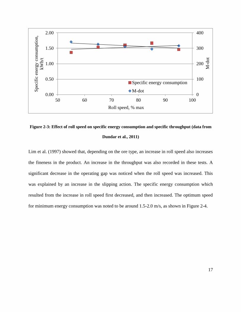
Based on the data provided by Dundar et al. (2011), specific energy and m-dot at different roll
speeds were calculated and plotted as shown in Figure 2-3.
17
Figure 2-3: Effect of roll speed on specific energy consumption and specific throughput (data from
Dundar et al., 2011)
Lim et al. (1997) showed that, depending on the ore type, an increase in roll speed also increases
the fineness in the product. An increase in the throughput was also recorded in these tests. A
significant decrease in the operating gap was noticed when the roll speed was increased. This
was explained by an increase in the slipping action. The specific energy consumption which
resulted from the increase in roll speed first decreased, and then increased. The optimum speed
for minimum energy consumption was noted to be around 1.5-2.0 m/s, as shown in Figure 2-4.
0
100
200
300
400
0.00
0.50
1.00
1.50
2.00
50 60 70 80 90 100
M-d
ot
Sp
ecif
ic e
ner
gy c
on
sum
pti
on
,
kW
h/t
Roll speed, % max
Specific energy consumption
M-dot

18
Figure 2-4: Effect of roll speed on specific energy consumption (Lim et al., 1997)
The difference between the plots shown in Figure 2-3 and Figure 2-4 can be explained by the
difference in the HPGR configurations used for the experiment. Dundar et al. (2011) analyzed
the effect of the roll speed using an industrial HPGR unit of 1700mm roll diameter and 850mm
roll width whereas Lim et al. (1997) used a laboratory scale HPGR of 250mm roll diameter and
100mm roll width. By increasing the roll diameter and width, the power draw through the HPGR
is increased significantly which in turns increases the net specific energy consumption.
Based on Figure 2-3 and Figure 2-4, the effect of roll speed on the specific energy consumption
is uncertain, simulations at different roll speed would be a way to analyze the response.

19
2.2.8 Pressure distribution on HPGR roll
One of the objectives for this research was to gain an understanding of the rock particle behavior
in an HPGR system. Using the developed model, the distribution of the hydraulic forces on the
particles under compression across the roll width was needed to understand this behavior.
In an HPGR unit, the hydraulic cylinder applies a force to the bearing that gets transmitted
throughout the roll surface. However, previous studies have shown that the distribution of the
pressure is not even throughout the roll width.
The compression angle (α) for an HPGR is defined as the angle where the feed material
experiences the pressure from the rolls whereas nip angle (β) indicates the region where no slip
occurs between particle bed and roll surface (Nadolski, 2012) as shown in Figure 2-5. Nip angle
is less than or equal to the compression angle.
Figure 2-5: Compression and nip angle in an HPGR (Nadolski, 2012)

20
Schönert and Sander (2002) suggested that the pressure on the HPGR roll surface drops with the
compression angle as shown in Figure 2-6. The maximum pressure is obtained at the center of
the roll where angle (α) is 0 degrees and decreases with the increase in the angle. It is also
concluded that the particle bed compression occurs till an angle of 10 degrees in the feed side
and it also drops to zero at an angle of 4 degrees when the product exits the compression zone.
Figure 2-6: Pressure distribution with compression angle (Schönert & Sander, 2002)
Lubjuhn (1992) has suggested that the pressure drop at the edge depends on the grinding force
and can drop by up to 75% when compared to the pressure at the center independent of the
material properties. Torres and Casali (2009) used this information and plotted the pressure
profile across the roll width as shown in Figure 2-7, where piE and pi
C are the product distribution
at the edge and the center respectively.

21
Figure 2-7: Pressure profile across roll width (Torres & Casali, 2009)
Nadolski (2012) used similar information to model the stress intensity across the roll width for
copper ore, as shown in Figure 2-8.
Figure 2-8: Pressure distribution across roll width (Nadolski, 2012)
22
2.3 Piston-die test
One of the greatest barriers to the faster adaptation of HPGR has been the lack of availability of
small lab-scale test procedures which use a few kilograms of sample in order to evaluate the
performance of HPGR and predict all levels of sizing information.
Piston-die tests are commonly used to study the inter-particle compression behavior of rocks. In
the past few years, various researchers have used piston-die pressing tests to predict sizing
information for HPGR. Hawkins (2007) used a piston and die arrangement to evaluate the
performance of a lab scale HPGR unit. She suggested that the piston and die test alone, or along
with lab scale HPGR tests, can be used to simulate industrial scale HPGR units.
Bulled et al. (2009) used a piston-die test, called a static pressure test (SPT), to estimate the
grindability index for HPGR and identified a high pressure grindability index which provided an
estimation of specific energy consumption for an HPGR unit.
Kalala et al. (2011) used different piston-die diameters to evaluate the breakage behavior of
particles. He used these tests to obtain the size distribution of a piston pressed product and
compared it with a lab scale HPGR product at different energy inputs. He also modified the flat
bottom piston arrangement to incorporate the edge effect that is observed in the HPGR
operations. A finer center product was obtained than the edge product for all the tapered piston
geometry tests.

23
Davaanyam et al. (2013) used a piston pressing method to correlate the piston-die test results
with a pilot-scale HPGR unit that could be used directly afterwards to size an industrial scale
HPGR unit.
The piston-die tests developed by Davaanyam et al. (2013) is more efficient in terms of
predicting the sizing and selection information of an industrial unit due to its direct correlation
with the pilot scale HPGR unit which has a 1:1 scale up factor rather than a laboratory scale unit.
2.4 Computer modelling and simulation
2.4.1 Introduction
Computer modelling is a technique used to gain an understanding regarding equipment and
particle behavior in any given system. It is difficult to formalize and run a test to understand
particle and equipment behavior under all machine and operating conditions. Understanding and
optimizing comminution equipment is expensive and time consuming and it also requires
considerable manpower and sample size (Delaney et al. 2010).
Computer models use real life machine setups and, based on the laws of physics, they analyze
the movement of different components which can further be used to simulate a variety of
operating conditions and predict the behavior of the machine. The outputs from the simulation
can be used for sizing, selection and optimization.

24
Various modelling approaches have been used in the past to study the behaviors of crushers
including cone crushers, jaw crushers, roll crushers and mills such as SAG mills, ball mills and
rod mills, as well as horizontal and vertical stirred mills.
Gupta et al. (1982) have suggested that the linearized population balance model can be used to
predict the size distribution of ball mill product. Soni et al. (2009) used the matrix method, which
includes selection and breakage functions, to simulate particle behavior in smooth double roll
crushers.
2.4.2 Discrete element method modelling
The modelling technique used for this research is the Discrete Element Method (DEM)
developed by Cundall and Stack (1979). They defined the Discrete Element Method as a
modeling technique used to simulate the behavior, interaction and motion of a collection of rigid
or deformable particles of arbitrary shape and size against each other. It uses individual particle
properties and their dynamic behavior to model movement and to trace the motion of the
particles.
DEM Modelling has successfully explained the particle breakage in tumbling mills such as ball
mills (Mishra & Rajamani, 1992), SAG mills (Cleary et al., 2003a), stirred mills (Cleary et al.,
2006).
Herbst et al.’s (2008) DEM based model is used to predict diamond liberation in kimberlitic ores
in an AG mill. Khanal and Morrison (2008) used DEM to model the abrasion breakage in a

25
tumbling mill using the collision and energy spectra. Potapov et al. (2007) used DEM and the
population balance model to simulate particle breakage in cone crushers. Murariu (2007) used
DEM to create a 3D model for the optimization of a magnetic roll separator.
Mishra and Thornton (2002) used DEM to simulate the ball mall and predict the torque on the
mill within 8% of the experimental results. Refahi et al. (2009) created a model for a jaw crusher
using DEM and compared the bond crushing energy with the energy required for single particle
breakage in the crusher. Abd El-Rahman et al. (2001) used DEM to predict the tumbling mill
power for industrial applications in order to study the effects of changes in lifters and other
design variations. Wang et al. (2012) investigated the collision energy, dissipated energy and
maximum impact energy in a ball mill and used it to predict product size distribution. Tavares
and de Carvalho (2009) modelled the breakage rate of particles in ball mills for batch grinding
using DEM.
Many other papers have also indicates that DEM has successfully simulated the power
consumption, liner geometry, particle motion and wear in different comminution units (Bwalya
& Moys, 2003; Cleary, 1998; Cleary & Hoyer, 2000; Cleary et al., 2001; Cleary et al., 2003b;
Hlungwani et al., 2003; Morrison et al., 2001; Morrison et al., 2007; Powell et al., 2003;
Rajamani & Mishra, 1996; Sinnott et al., 2006; Wang et al., 2012).
HPGRs, which are a relatively new type of comminution equipment, have only had a limited
numbers of papers written with respect to their DEM Modelling. Herbst et al. (2011)
implemented an energy-based population balance model and used discrete element method

26
modelling for the METSO ProSim flow-sheet simulator. Packed bed compression tests were
used to estimate selection and breakage function parameters and the trained model was used to
predict power, throughput and product size distribution. A DEM model for HPGR breakage can
be seen on the ROCKY (DEM Software) website. This model was used by Nordell and Potapov
(2011) to predict the difference in energy consumption between an HPGR and a Conjugate
Anvil-Hammer mill (CAHM).
Djordjevic and Morrison (2006) modelled the compressed particle bed using DEM and showed
that the stress intensity within the bed and particles increased with an increase in the applied
stress.
2.4.3 DEM basics
DEM uses a contact detection algorithm to find the particles that are in contact. Once the
contacts have been established, it uses various contact models (such as the Hertz-Mindlin contact
model) to calculate the contact forces (normal and tangential). Depending on the system which
needs to be modelled, various contact models are available including as the linear and hysteretic
spring models for elastic systems, linear cohesion and JKR (Johnson-Kandall-Roberts) cohesion
models for wet particles, and the Hertz-Mindlin model with heat conduction for heat transfer
systems (DEM Solutions, 2012).
Once the force is calculated, Newton’s second law of motion is used to trace the movement of
the particles. As shown in the Equation 2-4 and Equation 2-5,

27
Equation 2-4
(
| Equation 2-5
Where,
i and j are the interacting particles
vi = transitional velocity
ωi = angular velocity
Ii = moment of inertia
Ri = particle radius
Fn
ij = normal contact force
Ftij = tangential contact force
µr = coefficient of rolling friction
tor ue due to tangential forces
Based on these equations, the motion of the particles is traced, and movement is analyzed at each
time interval.

28
2.4.4 DEM modelling challenges
As a computer program, DEM inevitably uses intensive computational techniques. One of the
basic challenges is to incorporate the fine particles in the analysis. In any grinding equipment,
such as ball and SAG mills, the motion of the particles and mill behavior are highly depended on
the presence of fine particles. HPGR produces finer products than do any other types of crusher
equipment and its packed bed formation is due to the presence of fine particles in the sample or
fine particles generated during the crushing process. In the absence of fine, the particle bed will
not resemble the actual process which may render the model validation and sizing information
untenable. However, the analysis of the HPGR behavior under various operating conditions is
feasible.
The second important challenge is describing the comminution within the packed bed or creating
a particle breakage model for the packed bed. The population balance model and bonded particle
model only define the impact breakage realistically (Weerasekara et al., 2013).
2.4.5 Particle breakage modelling
Comminution is the process through which larger particles break into smaller particles through
the application of impact, shear or compression force. Implementing particle breakage into the
model is a difficult process while performing the modelling of any type of comminution
equipment. The breakage phenomenon depends highly on the nature of the forces, and the size
and shape of the particles.

29
In a modelling process, particle shapes and sizes are predefined that function as fixed parameters
and the phenomenon of particle breakage is defined accordingly so that the parent particle will
generate daughter particles of the same shapes and sizes that are predefined in the model, so that
the daughter particle have a definition for sequential breakage.
In actual particle breakage, the parent particles will break into irregularly shaped daughter
particles, and the sizes of the daughter particles can be estimated by lab tests which usually have
large ranges of size distribution (unlike the particle sizes, as pre-defined in the model).
Incorporating all the size ranges renders, the model complex and slow, hence, only a few size
fractions are considered for the modelling. This procedure makes it harder for any model to
accurately predict the real life behavior of equipment.
Various researchers have used different methods to incorporate particle breakage in a DEM
model. Thornton et al. (1996) used a large number of 2-dimensional discs (representing micro-
particles) in a region brought together by the application of a centripetal gravity force and
calibrated at a high, moderate and low velocity impact to model the breakage of agglomerates.
Potapov and Campbell (1994) employed triangular particles glued together to represent 2
dimensional particles, and assumed that if stress at any contact point exceeded a critical limit, the
glue would break and the crack would propagate accordingly. Potyondy and Cundall (2004) used
cluster of highly packed spherical rocks, called as meta-particles which were bonded together at
contact points and here breakage was represented by broken bonds based on the application of
stress. Hosseininia & Mirghasemi (2006) used the bonded particle/ meta-particle approach and
30
simulated particle breakage when the levels of shear, compressive or tensile stress were made to
exceed the allowable limit.
Delaney (2010) used a different approach where breakage conditions were first identified, and
then after the breakage of the parent particle occurred, it was then replaced by an appropriate
cluster of daughter particles.
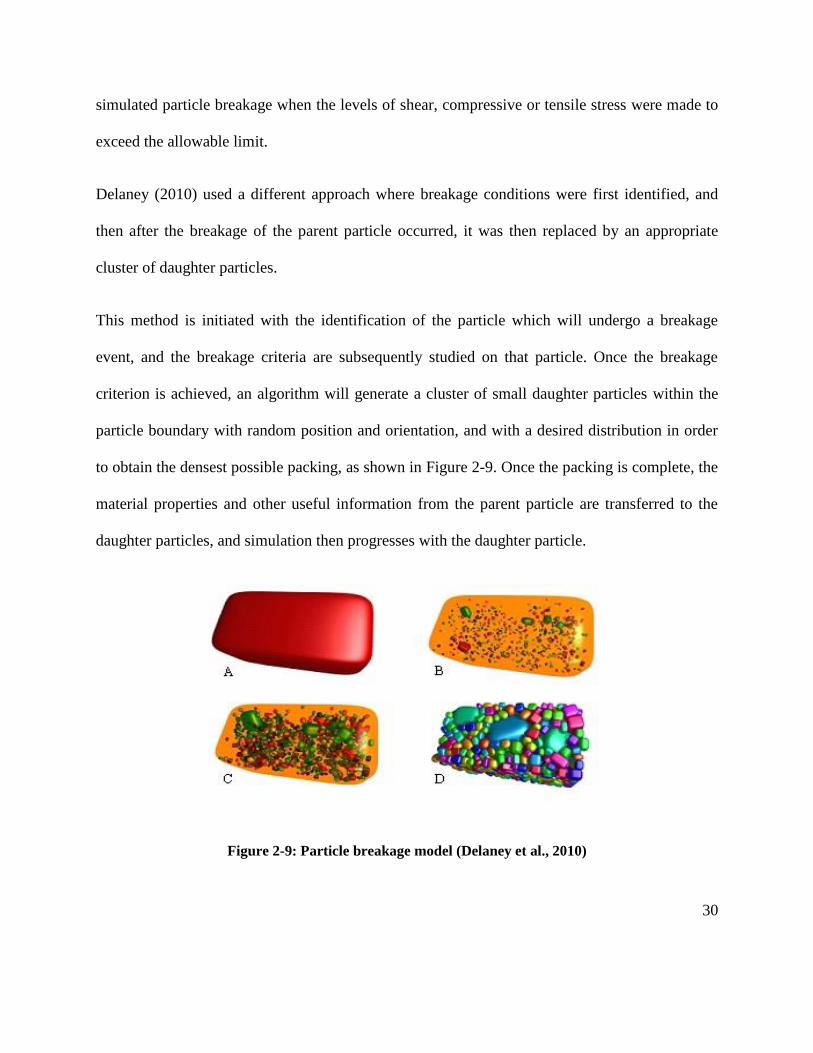
This method is initiated with the identification of the particle which will undergo a breakage
event, and the breakage criteria are subsequently studied on that particle. Once the breakage
criterion is achieved, an algorithm will generate a cluster of small daughter particles within the
particle boundary with random position and orientation, and with a desired distribution in order
to obtain the densest possible packing, as shown in Figure 2-9. Once the packing is complete, the
material properties and other useful information from the parent particle are transferred to the
daughter particles, and simulation then progresses with the daughter particle.
Figure 2-9: Particle breakage model (Delaney et al., 2010)

31
A similar approach is used for particle breakage modelling using spherical particles in this
research due to its simpler identification of the breakage criteria and particle replacement by the
densest packing distribution of the progeny.

32
CHAPTER 3: EDEM SOFTWARE AND MODEL SET-UP
The primary objective of this DEM-based research are to create a computer model to simulate
the conditions of a pilot-scale HPGR unit and to predict critical HPGR sizing information such
as energy consumption and m-dot, for certain samples and under certain machine operating
conditions.
There are five most basic steps involved in any modelling and simulation work which are listed
and explained below:
1. Physics of the model: Hertz-Mindlin contact model, which uses Newton’s laws of motion to
trace the particle movement, was used for this simulation. The details of the physics of the
model are available in section 3.3.1, 3.3.2 and 3.3.3.
2. Geometry and domain: Geometry for the model was created using Solidworks and EDEM
user’s platform. The domain defines the limit of the particles movement. The details of the
geometry and domain are available in section 3.3.5 and 3.3.8.
3. Boundary conditions: The physical boundaries of the model were defined by the geometry
of the system. The cheek plates and the HPGR rolls worked as the boundary for the particle
movement.
4. Initial conditions: Initial conditions for the simulation were limited to the choke and gravity
fed conditions for the feed particles. Initial conditions for the motion of the geometries are
explained in section 3.3.6.

33
5. Materials properties: EDEM software uses shear modulus, Poisson’s ratio and density as the
input parameter for the model. Section 3.3.4 includes the details for materials properties.
The Discrete Element Method (DEM) is a modelling technique used to simulate the behavior,
interaction and motion of a collection of rigid or deformable particles of arbitrary shape and size
against each other (Cundall & Stack, 1979). All DEM software works on the principle of contact
detection, force calculation and of tracing particle movements. All contact force data is saved
based on user requirements.
3.1 EDEM software
The DEM software used for this research work is EDEM, introduced by DEM solutions in 2005.
It is the one of the most flexible software options available for DEM modelling as the user can
modify and create custom codes to suit certain applications. The analysis loop for EDEM is
shown in Figure 3-1.
Figure 3-1: EDEM analysis loop (DEM Solutions, 2012b)
34
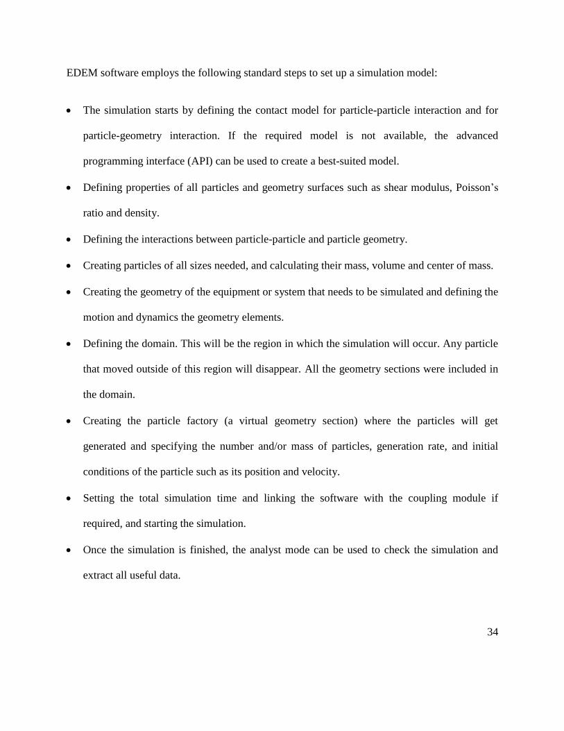
EDEM software employs the following standard steps to set up a simulation model:
The simulation starts by defining the contact model for particle-particle interaction and for
particle-geometry interaction. If the required model is not available, the advanced
programming interface (API) can be used to create a best-suited model.
Defining properties of all particles and geometry surfaces such as shear modulus, Poisson’s
ratio and density.
Defining the interactions between particle-particle and particle geometry.
Creating particles of all sizes needed, and calculating their mass, volume and center of mass.
Creating the geometry of the equipment or system that needs to be simulated and defining the
motion and dynamics the geometry elements.
Defining the domain. This will be the region in which the simulation will occur. Any particle
that moved outside of this region will disappear. All the geometry sections were included in
the domain.
Creating the particle factory (a virtual geometry section) where the particles will get
generated and specifying the number and/or mass of particles, generation rate, and initial
conditions of the particle such as its position and velocity.
Setting the total simulation time and linking the software with the coupling module if
required, and starting the simulation.
Once the simulation is finished, the analyst mode can be used to check the simulation and
extract all useful data.

35
The parameters studied in this research were roll speed and specific pressing force. The effect of
these parameters on operating gap, throughput, m-dot and energy consumption was analyzed.
3.2 Limitations of EDEM
As mentioned earlier, EDEM is the one of the most flexible software options available for DEM
modelling as the user can modify and create custom codes to suit certain applications. DEM, in
general, involves time-consuming computational techniques. The factors affecting the speed of
the simulation can be listed as:
Number of particles
Increasing the number of particles in a simulation increases the simulation time exponentially.
An HPGR pilot scale test requires approximately 250-300 kg of sample per test in order to obtain
enough stability to gather all the critical sizing parameters. The number of particles in a 250 kg
sample based on particle size can go in the billions, which is a huge number based on DEM
standards. All the simulations run for this research were kept to 25 kg sample mass in order to
drop the number of particles to approximately 100,000.
Size of the particles
Decreasing the particle size increases the number of particles for the same mass, and thus
decreases the simulation speed and increase the completion time. Based on the a paper published
by Nordell & Potapov (2011), DEM simulation can accurately model the grinding for particles of
up to 35mm size, as shown Figure 3-2.

36
Figure 3-2: HPGR simulation results from 100mm feed to 35mm product size (Nordell & Potapov,
2011)
Material parameters
According to the EDEM manual (2012b), simulation time increases exponentially with the
increase in the shear modulus of the particle, as shown in Figure 3-3. Increasing the shear
modulus of the particle increases the forces and stress intensity, that then results in a lower
timestep to capture these forces (Roufail, 2011). A simulation with a lower timestep will improve
the model behavior but it will also increase the total simulation time significantly.

37
Figure 3-3: Shear modulus vs. simulation run time (DEM Solutions, 2012b)
Complexity of the model
The complexity of the model can be defined in terms of the structure of user-defined codes, the
complexity in the geometry, use of different particle sizes at the same time, and particle shape.
User defined codes were used to extract force and pressure data between particle-particle and
particle-surface interactions, and to incorporate particle breakage in the model. All these
complex algorithms decrease the simulation speed and thus increase the simulation completion
time.
Simulation-runtime
Most of the simulations run for HPGR models were either very short in terms of time, or
information of the runtime was not provided. A simulation for the variation of roll width between

38
HPGR rollers provided by EDEM was run for approximately 3.8 seconds (DEM Solutions),
which is quite low in order to simulate pilot-scale HPGR performance.
Computer hardware
The processor used for this research was Intel(R) Core (TM) i7 – 3960X CPU @ 3.30 Ghz, 16.0
GB RAM, a 64-bit operating system which was one of the fastest portable computers available at
the time of purchase. However, its computational capacity is restricted. ROCKY (DEM
software) was run on a 32-core computer to model the comminution in HPGRs and mills
(Nordell & Potapov, 2011).
Even if using a higher processor speed, all the mentioned limitations would still function to limit
the validation of the model when compared to an actual pilot scale test. However, it should be
feasible to compare the trends of force, energy consumption or operating gap with the pilot scale
and use the correlations to estimate the sizing information.
3.3 Model set-up
Various models and interaction parameters needed to be set in order to create an HPGR and
piston-die model. All the interactions and parameters are included in this section.
3.3.1 Particle-particle interaction model
EDEM has various built-in contact models. The model used for this simulation was the Hertz-
Mindlin Contact Model (Figure 3-4). In this model, the normal force component is based on

39
Hertzian contact theory and a tangential force model is based on the work of Mindlin-
Deresiewicz (DEM Solutions, 2012).
Figure 3-4 illustrates the collision between the two particles A and B using a linear spring-
dashpot model which represents the elastic and non-elastic particle behavior. The total force
between the particles can be divided into normal and tangential forces. Spring and damping
components are available for both the forces, friction is available only for tangential component
and coefficient of restitution is related to the normal force component.
Figure 3-4: Schematic diagram for Hertz-Mindlin contact model (Roufail, 2011)
This model calculates the normal forces using material properties such as the coefficient of
restitution, Young’s modulus, Poisson’s ratio, size and mass, which can be expressed from
Equation 3-1 to Equation 3-7. All the equation provided was extracted from DEM solutions
manual (2012a).

40
√
Equation 3-1
Equation 3-2
Equation 3-3
√
√
Equation 3-4
(
)
Equation 3-5
√ Equation 3-6
√ Equation 3-7
Where,
Ei, vi, Ri, mi and Ej, vj, Rj, mj are Young’s modulus, Poisson’s ratio, radius and mass of the
particles in contact.

41
Fn = Normal force
E* E uivalent Young’s modulus
R*= Equivalent radius
m* = Equivalent mass
Fnd
= Normal damping force
vnrel
= Relative normal velocity
Sn = Normal stiffness
E = Coefficient of restitution
Also, in order to calculate the tangential forces, this model uses the shear modulus, tangential
velocities, coefficient of static friction and tangential stiffness as shown from Equation 3-8 to
Equation 3-10.
Equation 3-8
√ Equation 3-9

42
√
√
Equation 3-10
Where,
Ft = Tangential force
G*= Equivalent Shear modulus
Ftd = Tangential damping force
Vtrel
= Relative tangential velocity
St = Tangential stiffness
In the case of the rolling friction and torque calculation, angular velocities at contact are taken
into account and use Equation 3-11,
Equation 3-11
Where,
τi = Torque at the contacting surfaces
µr =Coefficient of rolling friction

43
Ri = Distance of the contact point from center of mass
ωi = Angular velocity vector of the particle at the contact point
According to DEM Solutions (2012), this contact model is the default model due to its accurate
and efficient force calculations. Advanced Programming Interface (API) module was used to
write codes in order to record the magnitude and direction of forces for further use as well as
calculations that are used for particle breakage.
3.3.2 Particle-geometry contact model
The Hertz-Mindlin Contact Model was used for particle and geometry interactions for HPGR
simulations. In order to analyze the distribution of the force on the rolls and piston-press, an API,
which records the pressure data at every timestep at each mesh point, was used.
3.3.3 Particle body force (breakage model)
The particle breakage model was created using the API in combination with Microsoft Visual
C++ Express. The model used for this purpose is the Particle Replacement Model in which
broken particles are replaced by smaller particles depending on their size.
A series of compression tests was conducted in order to measure the minimum force at which the
rock will break for a given size. The relationship between this minimum force and particle size
was determined for mineral samples and used as an input for the DEM model. The contact model
in EDEM calculates the force on each particle and compares it with the force value provided. As

44
soon as the force on the particle equals or exceeds the given minimum force value, it is moved
out of the simulation domain and replaced by daughter particles.
During the compression tests, it was observed that most of the particles have a tendency to break
in half. The particles having a shape closer to a sphere have two contact points, one with the
piston and other with the die. When such a particle is compressed, the crack initiates at the
contact point, propagates through the rock middle plane and fractures it into two identical half
sized rocks.
Since spherical particles are used for simulation purposes in order to reduce complexity and
improve simulation speed, the daughter particles were transformed into two particles in the next
smaller size range, as shown in Figure 3-5.
Figure 3-5: Particle replacement with two particles
When a particle is broken and replaced by its progeny, neighboring particles are pushed aside
due to the sudden change in particle size and volume. This can be likened to an explosion effect

45
and is not considered to take place during actual HPGR operation. In order to reduce this error,
the maximum force acting on the particle is restricted to a fraction of the breakage force for a
short period of time, allowing for the particles to separate. Based on the simulation, a time
interval of approximately 0.45 sec was found to suitably reduce this error. This phenomenon
renders the simulated environment stable, but also reduces the likelihood of duplicating the
actual process.
In order to minimize this occurrence, another system was created whereby, - a sphere of a size
representative of the particle to be replaced, - was filled up with maximum numbers of
predefined smaller sized particles similar to the particle replacement model presented by Delaney
(2010) as illustrated in Figure 3-6. This cluster was then used as the progeny. This method has
the limitation of having a longer simulation time, as the numbers of newly created particles are
much higher.
Figure 3-6: Particle replacement with cluster

46
3.3.4 Material properties and interactions
The primary objective of this research was to create a model which can be validated against the
pilot scale test results. In order to best approximate the real case, the material properties of
HPGR geometries and particles were kept similar as possible to the real scale tests.
Shear modulus, Poisson’s ratio and density were the three properties used by EDEM. Based on
the available literature, values for similar materials were obtained. Gereck (2007) and Stanford
(GEOL 615) have recorded some of the material properties and their interaction values that were
used for the purposes of simulation. The material properties used for the EDEM simulation are
listed in Table 3-1 below.
Table 3-1: Material properties
Materials Shear modulus (GPa) Poisson’s ratio Density (kg/m3)
Roll surface 78 0.29 7850
Particle (iron ore) 40 0.25 2880
Particle (copper ore) 31.2 0.25 2630
Density values used for particles which obtained from lab tests included the weight of the rock
dry and weight of rock in water. The weight of the rock in the water provides the volume of the
rock. By diving the dry rock mass by its volume, the density of the rock was determined.

47
Material interactions (particle to particle and particle to roll surface) values are listed in Table
3-2. The values for the material interactions are based on similar materials and were obtained
from the literatures and from various websites (2012) listed in the references.
Table 3-2: Particle and roll surface interactions
COR COSF CORF
Particle-particle 0.5 0.6 0.01
Particle-roll surface 0.5 0.45 0.01
Where, COR = co-efficient of restitution, COSF = co-efficient of static friction and CORF = co-
efficient of rolling friction.
3.3.5 HPGR geometry
The pilot scale HPGR consists of various geometrical sections which were designed separately,
and then used for simulation purposes. The important moving sections were created to
approximate those of the pilot scale machine available at UBC’s mining laboratory, whereas
other stationary parts were designed to ensure for uninterrupted particle flow. The motions of the
geometries were assigned based on the pilot scale tests operating conditions. If the geometry
used was made up of simple cubes or cylinders, it was created within the EDEM software
whereas complicated geometries such as the HPGR rolls were designed using computer-aided
design software.

48
The pilot scale unit available at the UBC mining laboratory has a roll diameter of 750mm, a roll
width of 220mm, and it is lined with HEXADUR® profile, as shown in Figure 3-7. A similar
structure was created using Solidworks (A CAD software) and then imported to EDEM for
simulation.
Figure 3-7: HPGR geometry from EDEM
As a result of their simple designs, the hopper, cheek plates and the feed chute were designed
within the EDEM software. The factory is the virtual geometry where the particles get created.
Generated particles were collected in the hopper, and were then fed to the HPGR under various
operating conditions.

49
3.3.6 Motion of geometries
Fixed roll movement
In the HPGR model, one of the rolls is fixed in a horizontal position and can easily be modelled
using EDEM geometry dynamics. A linear rotational motion was provided to this roll and the
angular speed was assigned according to the simulation requirements.
Floating roll movement
In the HPGR model, the roll which is able to move freely in the horizontal position according to
the forces of the particle bed and the opposing hydraulic forces is referred as a floating roll.
Special coding is required to model the more complex dynamics that are associated with the
floating roll. This code, which was developed in Microsoft Visual C++ Express, determines the
force values from EDEM, performs the mathematical calculations for the roll, and sends the new
roll position back to EDEM. The forces being exerted onto the floating roll are shown Figure
3-8, where Fx is the force on the roll due to the particles and FEXT is the force on the roll due to
hydraulics and X, Y, Z is the center of mass of the roll at any given time.

50
Figure 3-8: Forces on the floating roll
Considering the forces in the x-axis, the new position of the roll is calculated based on the forces,
using Newton’s e uation for motion, and Equation 3-12 to Equation 3-15,
Equation 3-12
Equation 3-13
Equation 3-14
Equation 3-15
An ‘if’ condition is applied to stop the further movement of the roll when the minimum distance
between the rolls, referred as the static gap, which is 9mm in the pilot unit established at UBC
Mining Engineering Department, is achieved as shown in Equation 3-16.

51
If (gap between two rolls <= 9 mm and Roller Velocity(x) < 0)
Roller Velocity = 0.0
Equation 3-16
The rotational motion of the floating roll was kept a constant, similar to the fixed roll, and had no
impact on the linear motion of the floating roll.
Feed chute movement
A linear translation motion was given to the chute gate. If the speed of the gate is kept too high,
it will create a bouncing effect on the falling particles as they hit the roll surface. Various
simulations were run to obtain the optimum speed at which this effect was minimized. The
optimum speed of the gate was found to be 0.5m/s and this value was kept constant for all the
simulations.
3.3.7 Base particle definition
For the purpose of a pilot scale HPGR test, the entire sample is crushed and screened at 32mm.
Hence, 32mm was maintained as the top size for the tests and a 2 screen series was used for the
upper and lower size limits for the particles created in EDEM. The upper and lower limits for
particle sizes along with the mean sizes are listed in Table 3-3 and Table 3-4. The mean sizes
were used as the particle diameter in the simulation.
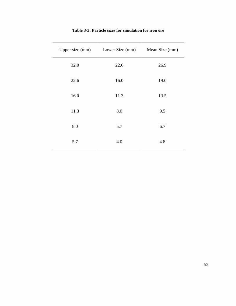
52
Table 3-3: Particle sizes for simulation for iron ore
Upper size (mm) Lower Size (mm) Mean Size (mm)
32.0 22.6 26.9
22.6 16.0 19.0
16.0 11.3 13.5
11.3 8.0 9.5
8.0 5.7 6.7
5.7 4.0 4.8

53
Table 3-4: Particle sizes for simulation for copper ore
Upper size (mm) Lower Size (mm) Mean Size (mm)
32.0 22.6 26.9
22.6 16.0 19.0
16.0 11.3 13.5
11.3 8.0 9.5
8.0 5.7 6.7
5.7 0.0 2.8
Using the particle properties listed in Table 3-1, particle volume, mass and moment of inertia
were calculated. Twenty-five kilograms of sample were used for each simulation.
3.3.8 Defining the domain
The domain of a model is the area in which the actual simulation will take place. The particles
and geometry inside this domain are analyzed. Once the particle goes outside of the domain area,
it disappears and the analyzer ceases to do estimates on its behavior.

54
In this model, the domain area was manually forced to be larger than the actual geometry area in
order to facilitate analysis and allow sufficient time for particles to stay in the domain before
they disappeared.
To establish the particle breakage phenomena, a large amount of sudden force is applied on the
parent particle that needs to be replaced so that it moves out of the domain and thus disappears.
3.3.9 Particle factory
A particle factory is a virtual geometry which defines, where, when and how the particles appear
in the simulation. As shown in Figure 3-7, the factory was placed above the hopper so that the
particles would gather in the hopper, and were then fed to the HPGR.
Each particle size has its own factory, which can be set as either dynamic or static particle
generation. The generation rate and number of particles can also be set. For this research, the
generation rate for each particle size, as well as the total number of particles were both kept
constant. No initial velocity was provided to the particles. Hence, the gravitational field was
responsible for their movement. The numbers of particles used for the purpose of the simulation,
determined using the mean size and the weight percentage of that size in the pilot scale HPGR
test feed, are listed in Table 3-5 below:

55
Table 3-5: Number of particles for simulation
Iron Ore Copper Ore
Mean Size (mm) No. of Particles Mean Size (mm) No. of Particles
26.9 22 26.9 126
19.0 111 19.0 853
13.5 1385 13.5 1867
9.5 6961 9.5 2353
6.7 17233 6.7 2535
4.8 6917 2.8 108389
Total 32607 Total 116123
A sample mass of 25 kg was used for all the simulations in order to reduce the simulation time
and to obtain sufficient data points for further analysis. In order to match the feed characteristics
of the pilot scale HPGR test, feed size distribution for simulation was kept similar to the pilot test
feed. A skewed feed distribution might improve the simulation time, but the simulation results
then can’t be used for validation due to difference in feed characteristics.

56
3.3.10 Particle breakage factory
The factory for particle generation during the breakage process is different than the normal
factory used for feed particle generation. This factory was compiled using the API module which
provides predefined size, number, position, orientation and other parameters for newly generated
particles. Both particle breakage methods have similar ways to generate new particles, except
with respect to the position reading of new particles with respect to the parent particles which got
replaced.
The API reads all the basic properties of the parent particle including its position, velocity and
orientation. Based on the type of replacement method used, it generates a number of new
particles and then places them in pre-assigned positions.
In the case of particle replacement with two particles, the position of the newly created particle is
calculated using Equation 3-17 and Equation 3-18,
X1 = XR + R, Y1 = YR, Z1 = ZR Equation 3-17
X2 = XR - R, Y2 = YR, Z2 = ZR Equation 3-18
Where,
X1, Y1, Z1 and X2, Y2, Z2 are the x, y, z positions of the new particles
XR, YR, ZR are the x, y, z positions of the replaced particle
57
R is the radius of the newly created particles (next smaller size fraction).
In the case of particle replacement with a cluster, the x, y, z position of the new smaller sphere
with respect of the replaced sphere is extracted from EDEM and the position of the new sphere is
given by Equation 3-19,
Xi = XR + xi, Yi = YR + yi, Xi = XR + xi and Zi = ZR + zi Equation 3-19
Where,
Xi, Yi, Zi are the x, y, z positions of the new particles
xi, yi, zi are the x, y, z positions of the new particles with respect of the replaced particles
XR, YR, ZR are the x, y, z positions of the replaced particle.
The orientation, linear velocity and angular velocity in different axes and planes are matched
with those of the replaced particles. Once all the information is assigned to the newly created
particles, the compiled factory creates the new sphere with those properties.
3.3.11 Timestep
The timestep is the amount of time between calculations. The smaller the timestep, the better and
more accurate the results will be, but, at the same time a small timestep also slows down the
simulation process.
58
A Rayleigh timestep, which is an idealized DEM timestep, is calculated based on the complexity
of the model by EDEM. A fraction of this time is used as a fixed timestep at which EDEM will
perform the actual calculations. Various simulations were run to analyze the timestep and an
optimum timestep was established for the whole simulation. As the particle fineness increases, a
smaller timestep needs to be set up in order to maintain accuracy.
For copper ore the fixed timestep used was 10% of the Rayleigh timestep whereas for iron ore it
was 20% of the Rayleigh timestep.
3.3.12 Simulation time
The simulation time equals the total simulation time for which the simulation will actually run.
No fixed time was used for this purpose. Simulations were stopped according to manual
observation when all the particles had passed through the rolls.

59
CHAPTER 4: EXPERIMENTAL PROCEDURES
This chapter includes detailed methodology, description of the sample used for the research and
the major equipment used to achieve the primary objective of the research. The major objective
of the research was to develop a computer model of an HPGR and analyze its behavior. In this
case, the results from the HPGR pilot tests on two different ore samples, copper and iron, were
used to validate the simulation results.
4.1 Methodology
In order to develop the computer model for HPGR for analyzing the behavior of the rocks in the
system and understanding equipment behavior under different machine operating conditions, an
experimental program was developed to generate the input data parameters for simulation.
Figure 4-1 shows a simplified flowsheet for the major components of the experimental
procedures.

60
Figure 4-1: Experimental program description
4.2 Sample description
Two samples from two different Canadian mines were identified for this research purpose. The
HPGR pilot results were performed within a two year window and enough feed samples were
available for further lab testing.

61
1. Copper ore deposit: A copper-porphyry sample with an average copper grade of 0.38%
copper and 0.007% molybdenum was used as one of the samples. Major minerals consisted
of chalcopyrite, bornite and pyrite, with quartz.
2. Iron ore deposit: The iron ore sample used for the test purpose contained approximately 30-
32% Fe mostly in the form of hematite with a small proportion of magnetite.
4.3 Pilot scale HPGR test
Actual pilot scale tests were not performed during this research work. The results from a total of
10 pilot tests performed earlier were directly used for analysis. However, the procedure for the
pilot scale HPGR tests is summarized here. All the tests were conducted using a pilot scale
HPGR manufactured by Koeppern Machinery Australia and installed at the UBC mining
engineering lab. The available HPGR is lined with a HEXADUR® lining profile designed by
Koeppern itself (Figure 4-2).
Figure 4-2: Pilot HPGR installed at UBC Mining Engineering (Wang, 2013)

62
All the HPGR tests were performed according to industrial standards. Table 4-1 summarizes the
technical specifications of this unit.
Table 4-1: Technical specifications of the pilot HPGR unit
Parameter Value Units
Roll diameter 750 mm
Roll width 220 mm
Main motor power 200 Kw
Maximum specific pressing force 8.5 N/mm2
Maximum roll speed 1.57 m/s
Roll wear liner HEXADUR ® -
Feed system Gravity -
The test procedure for a pilot scale HPGR test starts with screening the feed sample at 32 mm
and crushing the +32 mm to obtain 100% passing at 32mm. Crushed product and screen
undersize is homogenized using a rotary splitter and a representative sample for feed size
distribution and single particle compression testing is obtained.
63
All the testing parameters such as roll speed, pressing force, and moisture were adjusted and then
approx. 250-300 kg sample was used for the pilot test. Product from the stable operation was
split into a center and two edges, which were then sampled to obtain representative samples for
product size distribution. The product from the unstable operation was disregarded as waste. Roll
speed, power consumption, and operating gap were logged and analyzed to calculate critical
HPGR selection parameters such as specific energy and specific throughput. Product size
distribution was performed using lab scale screens to obtain the P80 and P50 numbers. The data
generated from these tests was used in the model for validation.
4.4 Single particle compression test
The major objective of the DEM modelling was to understand the behavior of rock particles in
an HPGR and predict its sizing information. In order to achieve the required objective, a particle
breakage model was needed to be introduced in the HPGR model which can reflect the
compression breakage. The single particle compression test was used as a means of introducing
particle breakage into the HPGR model. It measures the amount of compressive force required to
break a particle and then the measured force was used as an input parameter for the model.
This method was used to obtain the force value at which the rock had its first breakage. The test
was performed using the MTS hydraulic press as shown in Figure 4-3. The MTS load cell has a
rated hysteresis of +/- 325 Newtons.

64
Figure 4-3: MTS hydraulic press installed at UBC Mining Engineering
Representative feed samples from pilot scale HPGR tests were screened to obtain various size
fractions. The minimum size used for this test was 9.5 mm. Testing sizes lower than 9.5 mm as
single particles are impractical in MTS as the force value will be too low and the rock mass will
also be significantly low. The smaller rocks will have higher level of variation between the
particles which will render higher fluctuations in breaking force.
The number of rocks and the size fractions tested for the samples are listed in Table 4-2 below.

65
Table 4-2: Single particle compression test samples
Mean Size (mm) Upper size level (mm) Lower size level (mm)
Number of tests
(copper ore/iron ore)
28.51 32.00 25.40 15/5*
21.97 25.40 19.00 30/10*
17.44 19.00 16.00 30/20*
14.14 16.00 12.50 30/30
11.83 12.50 11.20 30/30
10.32 11.20 9.50 30/20*
*the iron ore sample was an AG mill product and fewer rocks with symmetrical shapes were
available in these size ranges.
For every size range, individual rocks were placed on a hardened steel plate. They were then put
into the MTS unit and pressed using displacement controlled movement. A fixed vertical
displacement rate of 1mm/min was used for all the tests. The displacement rate set-point was
kept low enough for slow compression breakage and to observe the rock breakage. Rocks were
pressed until breakage occurred at both their top and bottom contact surfaces. As for Point Load
Index (PLI) testing criteria, chipping and abrasion were not considered as breakage. Force values

66
were measured with a load cell and logged every 0.25 seconds. The peak force for a number of
equally sized particles was determined, and an average value was used as the breaking force to
obtain the relationship between breakage force and size. This value was then used in the HPGR
model.

67
CHAPTER 5: RESULTS AND DISCUSSIONS
This chapter summarizes the results of the single particle compression tests, results for the
HPGR pilot tests, predicted results from the simulation tests and their comparison with the actual
pilot scale HPGR tests.
5.1 Force and pressure distribution modelling
5.1.1 HPGR force distribution
As has been explained in literature review, the hydraulic force applied to the floating roll is not
evenly distributed across the roll width. The simulation tests performed using different specific
pressing forces were used to visualize the force acting on the particle near the center of the roll
geometry. Figure 5-1 shows the distribution of compressive force on the particles across the roll
width.
Due to the absence of the finer particles, the particle bed is not uniformly distributed. The red
spheres represent the particles experiencing maximum amount of force, green being the medium
force values and blue being the least amount of force on the particle. Figure 5-1 demonstrates the
compressive force distribution on the particles at different specific pressing force. Due to the
absence of fine particles in the system the distribution of force is not even in any given area.
However, it can be seen that at a specific pressing force of 2N/mm2, the combined number of red
and green particles is less than that at the specific pressing force of 3.5N/mm2. As the specific
pressing force increases from 2N/mm2 to 3.5N/mm
2, the number of blue particles in the central

68
region decreases and number of particles experiencing higher forces increases. This suggests that
increasing the specific pressing force increases the probability of breakage for a given particle. In
case of 3.5N/mm2, most of the particles having the forces in the green or above region will go
through a breakage event.
Figure 5-1: Compressive force on the particles at different pressing forces
Based on Figure 5-1, it can be concluded that by increasing the specific pressing force, the
compressive force on the particles would increase which in turns would improve the reduction

69
ratio. At the same time, it would also increase the linear wear rate and thus reduce the liner life.
By reducing the pressing force, liner life can be improved but at a trade of the reduction ratio.
The product size required for subsequent operation need to be analyzed in order to perform the
HPGR operation at an optimum pressing force and thus reducing the wear rate of the HPGR roll
surface. A trade off study between the wear rate and reduction ration would be needed to
estimate the optimum pressing force.
The figure also shows that the number of green and red particles for each specific force values is
higher near the center of the roll and decreases towards the edge. This suggests that the
concentration of the compressive force near the center of the roll is more than that near the
edges, which indicates that the particle towards the center of the roll have a higher probability of
breakage than the particle near the edge.
As can be seen in Figure 2-6, the pressure between a compression angle of 3 degrees towards the
feeding zone and 1 degree towards the product zone is significantly higher compared to higher
compression angles. The particles in this region, due to very high compression, were considered
for the analysis of force/pressure distribution across roll width.
Since the particle beds shown in Figure 5-1 are not uniformly distributed across the roll width, it
is harder to analyze the exact trend of the force/pressure distribution across the roll width.
However, the particle bed is more uniformly distributed at a specific pressing force of 3.5N/mm2
than the others; the values at this specific pressing force were used to plot the force/pressure
profile on the roll width.

70
Based on Figure 5-1, the compressive force values on the particles for 3 seconds with a timestep
of 0.1 seconds were extracted from the simulation for further analysis. The entire width of the
roll was subdivided into 11 zones and forces on the particles in each zones was analyzed and
averaged over the time.
Figure 5-2: Total compressive force on particles across roll width
Figure 5-2 shows that the compressive force on the particles near the edges of the roll is lower
than the center. This suggests that the pressure on the roll is higher at the center than the edges,
which concludes that the wear rate at the center will be higher at the center than the edges.
A worn out roll after 2,600 hours of operation at Cerro Verde mine in Peru (Koski et al., 2011) is
shown in Figure 5-3, which confirms the prediction of higher pressure towards the center of the
roll. It also suggests that major focus would be required on the central region on the roll liners as
the liner near the edge was still in better condition.
0
50
100
150
200
250
300
0 20 40 60 80 100 120 140 160 180 200 220
Com
pre
ssiv
e fo
rce,
kN
Roll width, mm
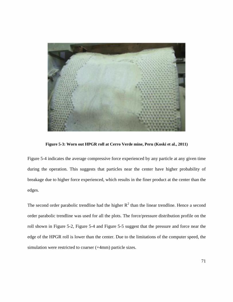
71
Figure 5-3: Worn out HPGR roll at Cerro Verde mine, Peru (Koski et al., 2011)
Figure 5-4 indicates the average compressive force experienced by any particle at any given time
during the operation. This suggests that particles near the center have higher probability of
breakage due to higher force experienced, which results in the finer product at the center than the
edges.
The second order parabolic trendline had the higher R2 than the linear trendline. Hence a second
order parabolic trendline was used for all the plots. The force/pressure distribution profile on the
roll shown in Figure 5-2, Figure 5-4 and Figure 5-5 suggest that the pressure and force near the
edge of the HPGR roll is lower than the center. Due to the limitations of the computer speed, the
simulation were restricted to coarser (+4mm) particle sizes.

72
Figure 5-4: Average compressive force on each particle across roll width
Figure 5-5: Average pressure on roll surface across the roll width
0
4
8
12
16
20
0 20 40 60 80 100 120 140 160 180 200 220
Co
mp
ress
ive
forc
e, k
N
Roll width, mm
0
100
200
300
400
500
0 20 40 60 80 100 120 140 160 180 200 220
Aver
gae
pre
ssure
, M
pa
Roll width, mm

73
The pressure on the HPGR rolls (Figure 5-5) is significantly higher than the observed pressure
during an HPGR operation due to the absence of fines. Due to the lack of fines, the coarse
particles were in direct contact with the roll surface and thus exerting a higher force on the rolls.
The finer size fractions in the samples would provide a cushioning effect, which in turns would
reduce the total force on the roll due to the particles and thus exert less pressure.
The distribution of the pressure and the magnitude of pressure drop also depend of the roll width.
A larger HPGR with bigger roll width is expected to have a higher drop in the pressure near the
edges. Increasing the roll width would increase the pressure drop at the edges, but it might also
stabilize the pressure profile across the roll width. A simulation with larger roll width would be a
way to analyze the force/pressure distribution in industrial scale HPGR rolls and to better
understand the optimum roll width to minimize the edge effect.
It also suggests that the simulations can be used to develop the pressure distribution curves
which will help to develop the piston geometries with similar profiles that will then be used to do
small lab scale piston tests. In order to improve the force profile, simulations with finer particle
sizes would be required over a longer time period.
5.1.2 Pressure distribution and piston geometry
Based on the information obtained by the simulations on HPGR and the pressure distribution
profiles, different piston geometries can be modelled in order to introduce the similar edge effect

74
in the piston-die tests (Kalala et al., 2011). Performing piston-die tests with tapered piston
geometry is one of the ways to introduce the edge effect.
Piston-die tests have been developed as the small scale test procedures for the HPGR sizing,
selection and performance analysis due to its lesser sample requirements (Davaanyam et al.,
2013). In order to further improve the laboratory scale test procedure using a piston-die and to
confirm the suitability of these tests for an HPGR analysis, the pressure profile in a piston-die
needs to be compared to the profile of an HPGR roll.
In order to analyze the pressure distribution across the floor of a die, elastic particles that were
infinitely compressible were used. As shown in Figure 5-6, a piston design with a variable
bottom angle similar to the one used by Kalala (2011) was incorporated in the 72 mm die and
pressed for a longer time period to obtain a steady pressure distribution that could be used to
evaluate the floor pressure.
Figure 5-6: Piston geometries (Kalala et al., 2011)

75
Since the software provides the pressure values at a single point, in order to have maximum
floor-particle contact points, randomly sized particles (2.6mm to 600 microns) were used. All the
four pistons shown in Figure 5-6 were moved down in a die from a given height, and pressure
data was recorded at the same time in all the cases. The distribution of pressure for all cases is
shown from Figure 5-7 to Figure 5-10.
The pressure values are substantiality higher than the values seen in HPGR (Figure 5-5) due to
the elastic nature of particles used to analyze the pressure profile and higher pressing duration
time without stopping the piston at any given force.
Figure 5-7: Floor pressure distribution with piston-1
0
20
40
60
80
100
-35 -30 -25 -20 -15 -10 -5 0 5 10 15 20 25 30 35
Pre
ssure
, M
Pa
(x10
6)
Die floor from center, mm

76
Figure 5-8: Floor pressure distribution with piston-2
Figure 5-9: Floor pressure distribution with piston-3
0
20
40
60
80
100
-35 -30 -25 -20 -15 -10 -5 0 5 10 15 20 25 30 35
Pre
ssu
re,
MP
a (x
10
6)
Die floor from center, mm
0
20
40
60
80
100
-35 -30 -25 -20 -15 -10 -5 0 5 10 15 20 25 30 35
Pre
ssure
, M
Pa
(x10
6)
Die floor from center, mm

77
Figure 5-10: Floor pressure distribution with piston-4
The results obtained by Kalala (2011) also suggested having a finer product size distribution at
the center of the piston and a coarser product size distribution at the edges. This concluded the
pressure drop seen in the pressure profile obtained by changing the bottom angle and a reduced
force near the die edges.
The pressure values at all the points were exported from the model and were plotted with the
distance of the point form the center of the die. A trendline that provides the maximum R2 was
added to the points in order to analyze the distribution. It was seen that the second order
parabolic trendline had the higher R2 than the linear trendline. Hence a second order parabolic
trendline was used for all the plots.
0
20
40
60
80
100
-35 -30 -25 -20 -15 -10 -5 0 5 10 15 20 25 30 35
Pre
ssu
re,
MP
a (x
10
6)
Die floor from center, mm

78
From the plots obtained from the pressure distribution at the die floor, it can be seen that
introducing a tapered bottom piston increases the edge effect as seen in HPGR roll pressure
profiles. It also concluded that changing the bottom angle for a piston can be a possible way to
introduce the edge effect in the piston-die test. Further laboratory scale tests using tapered
bottom would be required to confirm the suitability of this procedure.
Based on the pressure profile on the roll of a given HPGR obtained from the simulation, a
suitable piston geometry that matches the pressure profile of the HPGR can be derived and can
be used to perform the piston-die test at different energy levels in order to estimate the product
size distribution for an industrial scale HPGR unit.
It can be concluded that edge effect can be considered in the piston test. Depending on the HPGR
roll geometry (width), the appropriate piston design can be determined.
5.1.3 Pressure distribution and particle size
A study was conducted to analyze the effects of particle size on the pressure transmitted to the
floor of the die. The die was filled with rigid particles of three different particle sizes (-
12.5+11.2mm, -6.7+5.6mm, -2.8+2.0mm) with a constant total volume of 240ml. A cylindrical
piston was placed at approximately the same height from the particle bed (closest to the material)
and a velocity of 0.5mm/sec was provided to the piston. The speed at which the piston moves
downwards in a die, does not affect the results. Lower speeds increases the simulation time
hence, in order to record enough data points, a sufficiently slow speed was used.

79
The pressure at the die floor was visualized at 1, 4, 8, 12 seconds, as shown from Figure 5-11 to
Figure 5-22. Each dot represents a particle-die contact point.
It can be seen from Figure 5-11, that in the case of the coarsest particle (-12.5+11.2mm), the
figure has a higher number of red dots compared to green at 1 second, which suggests that the
force from the piston is transmitted to the die floor effectively. The number of red dots at 1
second is lower in the intermediate size fraction than the coarsest fraction (Figure 5-12) and
drops down to almost negligible for finest size fraction (Figure 5-13). This suggests that the force
from the piston is not able to get transmitted to the die floor.
Figure 5-11: Die floor pressure at 1 second (-12.5+11.2mm)
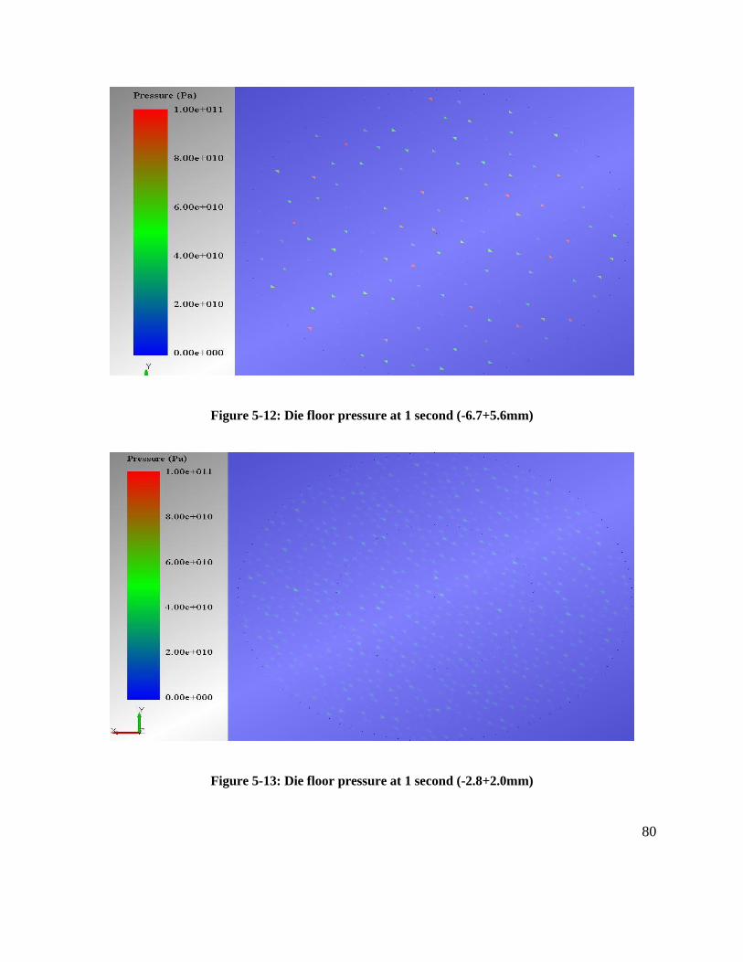
80
Figure 5-12: Die floor pressure at 1 second (-6.7+5.6mm)
Figure 5-13: Die floor pressure at 1 second (-2.8+2.0mm)

81
Figure 5-14: Die floor pressure at 4 seconds (-12.5+11.2mm)
Figure 5-15: Die floor pressure at 4 seconds (-6.7+5.6mm)

82
Figure 5-16: Die floor pressure at 4 seconds (-2.8+2.0mm)
Figure 5-17: Die floor pressure at 8 seconds (-12.5+11.2mm)

83
Figure 5-18: Die floor pressure at 8 seconds (-6.7+5.6mm)
Figure 5-19: Die floor pressure at 8 seconds (-2.8+2.0mm)

84
Increasing the time duration, increases the number of red dots for every size fraction. At 12
seconds, all the points for all three size fractions are red suggesting that the force is now getting
transmitted to the die floor as shown in Figure 5-20, Figure 5-21 and Figure 5-22.
Figure 5-20: Die floor pressure at 12 seconds (-12.5+11.2mm)

85
Figure 5-21: Die floor pressure at 12 seconds (-6.7+5.6mm)
Figure 5-22: Die floor pressure at 12 seconds (-2.8+2.0mm)

86
The software provides the pressure values at the points at which the particle is in contact with the
die floor. From Figure 5-11 to Figure 5-22 , it can be concluded that during the first few seconds,
most of the force applied by the piston is utilized for particle rearrangement, especially for the
smaller-sized particles. Since, the number of particles for the smallest sized fraction is
significantly larger than for the biggest particles, pressure at the die floor is significantly lower
for the -2.8+2.0 mm size fraction compared to coarser sizes. Once the rearrangement process is
completed, the force from the piston can easily get transmitted through the compacted particle
bed to the die floor as can be shown in Figure 5-20, Figure 5-21 and Figure 5-22.
Also, the finer particles provide higher levels of cushioning effect to the force transmission than
do the larger particles, which inhibit the piston force from transmitting to the die floor. For a
particle bed consisting of fine sized particles, the particle rearrangement will take longer time
compared to the coarse particle bed and thus the particles can keep getting compressed. Once the
bed is fully compacted, the piston force can easily get transmitted through the compacted bed to
the die floor.
In an HPGR application, finer particles have similar effect as the piston press. It helps in creating
the packed particle bed and provides the cushioning effect to the larger particles. The time spent
by the particle bed in the compression zone is very small which is not sufficient enough for
particle rearrangement and breakage, hence, it can be concluded that the finest fraction will pass
through the HPGR without much size reduction.

87
In order to analyze the pressure distribution trends of the particle bed, particle breakage was not
incorporated into the piston models. Hence, the energy usage in the piston-die, that uses the
force-displacement curve to calculate the energy, was not estimated.
5.2 HPGR tests and simulation analysis
HPGR pilot tests results were used as reference data points and were then used to validate the
results from the HPGR model. A correlation was established between the simulated results and
the pilot scale results to predict critical sizing information such as m-dot and specific energy
consumption.
5.2.1 HPGR pilot testing results
Results from a total of 10 pilot tests performed at the UBC Coal and Mineral Processing
Laboratory were used to analyze the effects of specific pressing force and roll speed. These
results were obtained by performing HPGR pilot scale tests based on industrial standards. These
data can be used directly to size and select the industrial scale HPGR unit. A summary of the test
results is listed in Table 5-1. A complete data sheet for these tests is included in Appendix A.

88
Table 5-1: HPGR pilot scale test results summary
Test No. Fsp
Roll
speed
M-dot Esp net
Operating gap Throughput
(N/mm2) (RPM) (mm) (tph) (ts/hm
3) (kWh/t)
IO 1 3.5 19.10 17.42 26.20 210 1.89
IO 2 2.5 19.10 18.25 26.90 215 1.44
IO 3 2.0 19.10 18.59 27.86 223 1.20
IO 4 2.0 19.10 18.02 28.70 229 0.99
IO 5 2.0 12.73 18.16 19.50 234 0.94
IO 6 2.0 25.47 18.20 38.90 234 0.95
CO 1 5.0 19.10 17.68 24.78 200 2.35
CO 2 4.0 19.10 18.09 24.81 196 1.98
CO 3 3.0 19.10 18.30 24.86 200 1.57
CO 4 2.0 19.10 21.01 26.17 210 1.15
(IO – iron ore, CO – copper ore; IO 1, 2 and 3 were run on scalped feed @ 4mm)

89
Based on the results listed in Table 5-1, the effect of specific pressing force on net specific
energy consumption and m-dot can be generated. In order to analyze the effects of the specific
pressing force and roll speed on the net specific energy consumption and m-dot, and to further
use it as validation criteria for the model, the following graphs were plotted.
An increase in specific pressing force increases the net specific energy consumption and
decreases the m-dot value linearly as shown in Figure 5-23 and Figure 5-24 respectively. Similar
results were obtained by Wang (2013).
From Table 5-1, it can also be concluded that the operating gap decreases with the increase in the
specific pressing force and increases with the increases roll speed.
Figure 5-23: Effect of specific pressing force on net specific energy consumption
0.0
0.5
1.0
1.5
2.0
2.5
1.5 2 2.5 3 3.5 4 4.5 5 5.5
Net
spec
ific
ener
gy c
onsu
mpti
on,
kW
h/t
Specific pressing force, N/mm2
Iron ore
Copper ore

90
Figure 5-24: Effect of specific pressing force on specific throughput constant
The effect of roll speed on net specific energy consumption and m-dot is not very significant
over the range of speed tested as shown in Figure 5-25. In order to analyze the impact of roll
speed, more pilot scale tests with higher and lower speeds will be required.
0
60
120
180
240
300
1.5 2 2.5 3 3.5 4 4.5 5 5.5
M-d
ot,
ts/
hm
3
Specific pressing force, N/mm2
Iron ore
Copper ore

91
Figure 5-25: Effect of roll speed on net specific energy consumption and specific throughput
constant
5.2.2 Single particle compression testing results
Single particle compression test were carried out to analyze the minimum force requirement to
break a particle for a given size and for a given ore type. These tests were developed to
determine the breakage parameter for compression breakage in a similar manner that the JK
DropWeight test used to assess the impact breakage parameters. Using similar standards as JK
DropWeight test, mono-sized samples were screened from the samples and 10-30 rocks from
each size fraction, depending on the rock size, were slowly compressed in a piston-press until its
fracture and the force value at the breakage was recorded.
The complete test results from single particle compression tests and force data can be seen in
Appendix B. The variations in the threshold force for the same sample and similar particle size
0
60
120
180
240
300
0.0
0.5
1.0
1.5
2.0
0 5 10 15 20 25 30
M-d
ot,
ts/
hm
3
Net
spec
ific
ener
gy c
onsu
mpti
on,
kW
h/t
Roll speed, rpm
Net Energy consumption
M-dot

92
range reflects the variation in the strength of the rocks due to their different composition. The
relationship between the minimum breakage force and the size of the particle can be seen in
Figure 5-26 and Figure 5-27.
Figure 5-26: Single particle compression test result (iron ore)
Figure 5-27: Single particle compression test result (copper ore)
1000
3000
5000
7000
0.0 5.0 10.0 15.0 20.0 25.0 30.0 35.0
Th
resh
old
forc
e, N
Particle size, mm
1000
3000
5000
7000
0.0 5.0 10.0 15.0 20.0 25.0 30.0 35.0
Thre
shold
forc
e, N
Particle size, mm

93
The trendline was used to estimate the threshold forces for the particle size used in the simulation
and then used as an input parameter in the particle breakage modelling codes.
A linear relationship was found between the force at which a particle experiences its first
breakage and its original size. When the individual threshold force for a given size particle was
normalized with the mass of the corresponding rocks to obtain force dissipated per gram of rock,
an exponential decreasing trend was obtained as shown in Figure 5-28. Since the particle size is
an indicator for the particle mass, the force vs. size curve was used as an input parameter for the
model. It can be seen that force per unit mass for iron ore is lesser than that for copper ore. Since,
the iron ore sample was an AG mill product, it was weaker compare to the copper ore which was
as SAG mill feed.
As shown in Figure 5-28, increasing the rock size, decreases the force acting on a unit mass of
the rock exponentially. The plot confirms that when rocks get bigger, the normalized force value
decreases and becomes nearly constant. At the same time, when the rocks get smaller, the
normalized force value increases and becomes so high that it will be nearly impossible to break
the rock by compression.
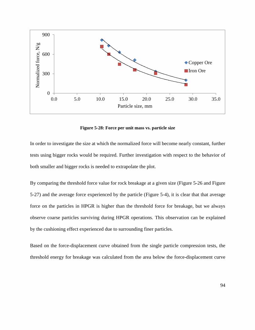
94
Figure 5-28: Force per unit mass vs. particle size
In order to investigate the size at which the normalized force will become nearly constant, further
tests using bigger rocks would be required. Further investigation with respect to the behavior of
both smaller and bigger rocks is needed to extrapolate the plot.
By comparing the threshold force value for rock breakage at a given size (Figure 5-26 and Figure
5-27) and the average force experienced by the particle (Figure 5-4), it is clear that that average
force on the particles in HPGR is higher than the threshold force for breakage, but we always
observe coarse particles surviving during HPGR operations. This observation can be explained
by the cushioning effect experienced due to surrounding finer particles.
Based on the force-displacement curve obtained from the single particle compression tests, the
threshold energy for breakage was calculated from the area below the force-displacement curve
0
300
600
900
0.0 5.0 10.0 15.0 20.0 25.0 30.0 35.0
Norm
aliz
ed f
orc
e, N
/g
Particle size, mm
Copper Ore
Iron Ore

95
until fracture point and dividing it by the mass of the rock. This threshold force indicates the
minimum energy required to break a particle of a given size.
Figure 5-29 and Figure 5-30 shows the relationship of threshold energy for breakage and particle
size with 95% confidence intervals. It can be concluded that the threshold energy decreases with
the increase in the particle size. Further testing using different ore samples would be required to
confirm the nature of the plot.
Figure 5-29: Threshold energy vs. particle size for iron ore (Nadolski et al., In press)

96
Figure 5-30: Threshold energy vs. particle size for copper ore (Nadolski et al., In press)
As can be seen from the plots, the value of the threshold energy is significantly lower than the
energy consumption in a tumbling mill or an HPGR. Threshold energy, for a given particle size,
is the minimum energy required to impart breakage to the rock (Nadolski et al., In press). These
energy values can be used to investigate into more efficient comminution equipment. These
results can be further used to develop a performance index (Equation 5-1) for comminution
equipment by comparing the threshold energy for the rock to the actual energy consumed in the
actual operation. This index would be able to provide a benchmark for the rock breakage and
estimate the efficiency of the comminution unit.
Equation 5-1

97
The test also suggests that the single particle compression tests is an effective method to analyze
the breakage parameters and can be further used to generate the energy-size relationship for
compression breakage & similar procedure was developed by Davaanyam et al. (2013) to create
the small scale procedure for HPGR sizing and selection by using a piston-die test.
5.2.3 DEM model results
Simulations were run for the ore samples at different pressing forces and roll speeds to observe
their effect on the dynamic gap between the roll surfaces. As described in section 3.3.7, a sample
size of 25 kg was used for the simulation. The variation in operating gap with time shown in
Figure 5-31 to Figure 5-33 indicates that, for iron ore, it took 2 seconds for the floating roll to
reach the steady state and by 5 seconds the sample was becoming depleted. In the case of the
copper ore, the stable region was not obtained. However, the 2 to 4 second region was used for
the purposes of this study. A simulation with more sample mass over a longer period of may
provide steady and stable operation. For the speed variability test, the operating gap stability was
found to be different for different speeds.

98
Figure 5-31: Operating gap vs. time at different pressing force (iron ore)
Figure 5-32: Operating gap vs. time at different roll speed (iron ore)
0
5
10
15
20
25
30
0 1 2 3 4 5 6 7 8
Op
erat
ing g
ap,
mm
Time, sec
2 N/mm2
2.5 N/mm2
3.5 N/mm2
0
5
10
15
20
25
30
0 2 4 6 8 10 12
Oper
atin
g g
ap,
mm
Time, sec
10.0 rpm15.0 rpm19.1 rpm25.0 rpm35.0 rpm
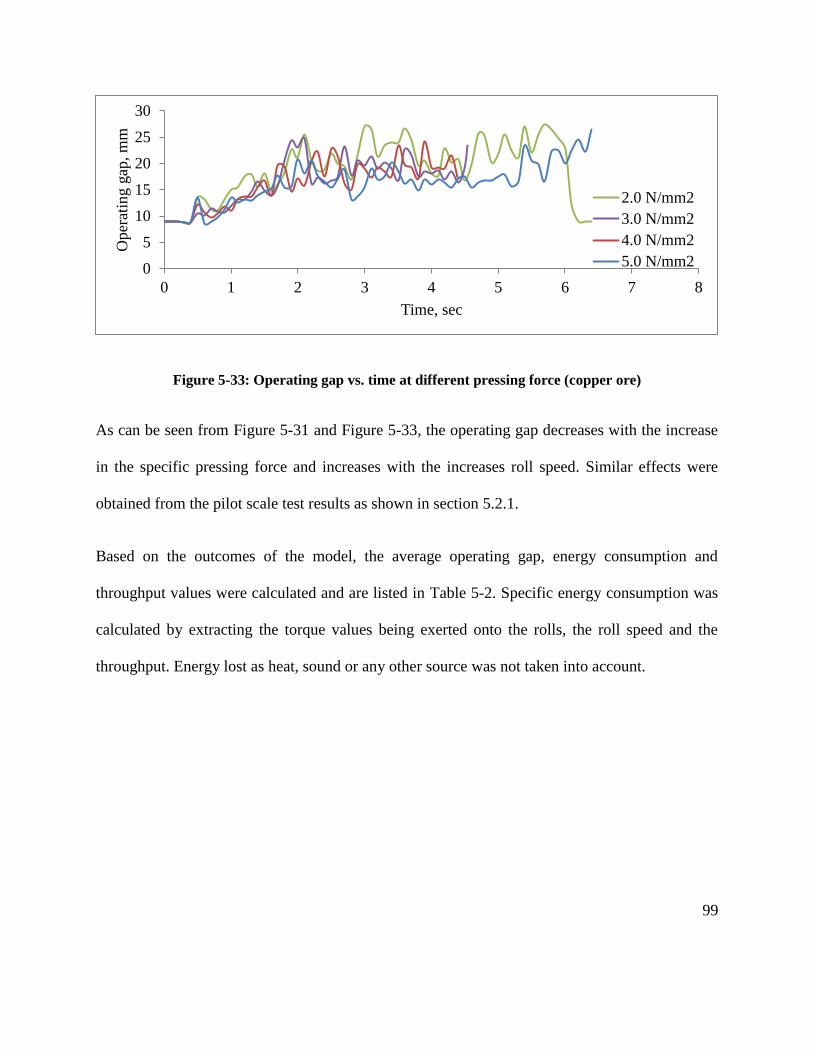
99
Figure 5-33: Operating gap vs. time at different pressing force (copper ore)
As can be seen from Figure 5-31 and Figure 5-33, the operating gap decreases with the increase
in the specific pressing force and increases with the increases roll speed. Similar effects were
obtained from the pilot scale test results as shown in section 5.2.1.
Based on the outcomes of the model, the average operating gap, energy consumption and
throughput values were calculated and are listed in Table 5-2. Specific energy consumption was
calculated by extracting the torque values being exerted onto the rolls, the roll speed and the
throughput. Energy lost as heat, sound or any other source was not taken into account.
0
5
10
15
20
25
30
0 1 2 3 4 5 6 7 8
Op
erat
ing g
ap,
mm
Time, sec
2.0 N/mm2
3.0 N/mm2
4.0 N/mm2
5.0 N/mm2

100
Table 5-2: HPGR modelling results summary
Ore Fsp Roll speed
Operating
gap Throughput M-dot Esp net
(N/mm2) (RPM) (mm) (tph) (ts/hm
3) (kWh/t)
Iron 3.5 19.10 13.00 18.38 148.55 1.37
Iron 2.5 19.10 13.64 18.81 152.00 0.87
Iron 2.0 19.10 14.09 18.46 149.17 0.82
Iron 2.0 10.00 13.18 11.71 180.20 0.63
Iron 2.0 15.00 14.15 16.41 168.94 0.69
Iron 2.0 19.10 14.09 18.46 149.17 0.82
Iron 2.0 25.00 14.39 23.75 146.51 0.83
Iron 2.0 35.00 15.20 28.16 124.01 1.03
Copper 5.0 19.10 16.98 20.54 166.01 1.37
Copper 4.0 19.10 19.23 21.73 175.62 1.12
Copper 3.0 19.10 19.26 22.20 179.37 0.85
Copper 2.0 19.10 21.65 22.26 179.86 0.54

101
Data collected from the simulation results are shown in Figure 5-34 and Figure 5-35 that
demonstrate that the effect of the specific force on m-dot and specific energy consumption can
be observed by the computer model. An increase in the specific pressing force increases the
specific energy consumption and decreases the m-dot. It can also be concluded that the
simulation results generate similar trends to those observed in a pilot scale test. The magnitudes
of the m-dot and net specific energy consumption are lower that is further analyzed in section
5.2.4.
Figure 5-34: Simulated effect of specific pressing force on net specific energy consumption
0.0
0.2
0.4
0.6
0.8
1.0
1.2
1.4
1.6
1.5 2 2.5 3 3.5 4 4.5 5 5.5
Net
spec
ific
ener
gy c
onsu
mpti
on,
kW
h/t
Specific pressing force, N/mm2
Iron ore
Copper ore

102
Figure 5-35: Simulated effect of specific pressing force on specific throughput constant
Figure 5-36: Simulated effect of roll speed on net specific energy consumption and specific
throughput constant for iron ore
0
60
120
180
240
300
1.5 2 2.5 3 3.5 4 4.5 5 5.5
M-d
ot,
ts/
hm
3
Specific pressing force, N/mm2
Iron ore
Copper ore
0
60
120
180
240
300
0.0
0.5
1.0
1.5
2.0
0 10 20 30 40
M-d
ot,
ts/
hm
3
Net
spec
ific
ener
gy c
onsu
mpti
on,
kW
h/t
Roll speed, rpm
Net Energy consumption
M-dot

103
Due to the narrow roll speed ranges tested in the pilot scale, the effect of the roll speed from the
pilot test was not established as shown in Figure 5-25. From Figure 5-36, a trend similar to
Figure 2-3 can be observed for specific energy consumption and m-dot with respect to roll speed
for a longer range of roll speed. Based on these figures, it can be concluded that over a longer
range of increasing speed tests a decreasing effect on m-dot and an increasing effect on energy
consumption will be obtained.
5.2.4 Model vs. pilot scale results
This section provides a detailed comparison between the data obtained from the pilot scale
HPGR test and the results obtained from the simulations.
Operating gap
In the case of iron ore, as shown in Figure 5-37, the operating gap values for iron ore determined
from the simulation were found to be lower than those measured through pilot scale testing
whereas, for the copper ore, the operating gap values determined from the simulation were closer
to the pilot scale tests under same machine conditions.

104
Figure 5-37: Operating gap (pilot scale vs. modelled results)
The deviation was considered because of two major reasons. The major reason for the deviation
is the absence of finer particles in the simulation. Finer particles help to create a packed bed
between the rolls and provide a cushion effect and thus expand the operating gap. Since, the
copper ore simulation used finer particles than the iron ore simulation, it produced a better
correlation.
Also, the deviation can be caused as the result of the proportion of the simulated particles
passing through the physical boundary of the rolls and bypassing the roll gap due to a relatively
higher time step size which caused the decrease in the operating gap. In DEM, the force
calculated on a particle is based on the particle contact overlap which represents the deformation
of the particle. Due to high forces and a longer time step, the particle overlap gets higher than the
12.0
14.0
16.0
18.0
20.0
22.0
12.0 14.0 16.0 18.0 20.0 22.0
Act
ual
Oper
atin
g g
ap,
mm
Simulated Operating gap, mm
Iron ore
Copper ore

105
particle radius and the particle passes through the boundary. In reality, the particle will likely
break, and not deformed that results in underestimation of the gap by simulation.
The results for the iron ore have shown that a strong correlation does exist between modelled and
measured values. The actual operating gap is 30% higher than the simulated operating gap.
With the presence of finer particles, it can be assumed that the simulated operating gap will be
closer to the actual gap. However, more simulations with finer particles needed to be performed
to evaluate the effect.
Throughput and m-dot
The throughput and m-dot from the simulation were found to be lower than the results measured
in the pilot scale tests. The difference in results is due to the model’s use of spherical particles,
which do not capture the packing characteristics of actual mineral samples and display a higher
sliding effect than the actual test. As shown in Figure 5-24 and Figure 5-35, a similar trend was
obtained for pilot scale and computer model results.
Table 5-3, it is clear that the presence of a finer particle size in the simulation significantly
reduces the deviation between the actual and modelled results. Throughput for an HPGR unit is
highly dependent on the operating gap. For a smaller operating gap, less material will pass
through at a given time and hence throughput will be lower.

106
Table 5-3: Throughput and m-dot (pilot scale vs. modelled results)
Test No. Throughput (tph) M-dot (ts/hm
3)
Actual Simulated % Difference Actual Simulated % Difference
IO 1 26.20 18.38 29.8 210 149 29.0
IO 2 26.90 18.81 30.1 215 152 29.3
IO 3 27.86 18.46 33.7 223 149 33.2
Average 31.2 30.5
CO 1 24.78 20.54 17.1 200 166 17.0
CO 2 24.81 21.73 12.4 196 176 10.2
CO 3 24.86 22.20 10.7 200 179 10.5
CO 4 26.17 22.26 14.9 210 180 14.3
Average 13.8 13.0
As shown in Figure 5-37, the simulated operating gap for iron ore is lower than the actual gap
which in turn reduces the throughput and hence a higher deviation is observed. In case of the
copper ore, the simulated operating gap is closer to the actual gap, hence the deviation is lower.

107
Product size distribution
The product size distributions for the actual pilot tests and simulation are shown in Figure 5-38
and corresponding percent passing 80 and percent passing 50 values are listed in Table 5-4. The
modelled HPGR product size distributions were analyzed for the time period ranging from 2 to 5
seconds, where simulated machine conditions were considered to be stable. Since the minimum
particle size was 4mm, product size distribution down to 4 mm is shown in the figure. The
product size distribution for iron ore was used as an example due to the greater stability of the
operating gap during simulation.
Figure 5-38: Product size distribution for iron ore (pilot scale vs. modelled results)
From Figure 5-38, it is clear that the product size distribution from the model is coarser than the
actual product. The explanation behind the coarser product size distribution might be due to the
0
20
40
60
80
100
1 10 100
Cum
. per
cent
pas
sing,
%
Particle size, mm
2.0 N/mm2 (Sim)
2.5 N/mm2 (Sim)
3.0 N/mm2 (Sim)
Feed (Sim)
Feed (Pilot)
2.0 N/mm2 (Pilot)
2.5 N/mm2 (Pilot)
3.0 N/mm2 (Pilot)

108
weakness of the particle replacement model used for the particle breakage. The particle
replacement model used for the research replaces the parent particles by a cluster of smaller
spheres rock size. Since, the smallest size of particle was 4mm, the parent particles were being
replaced by a cluster of daughter particles of sizes equal to or greater than 4 mm, which in turns
created a coarser product size distribution than the actual operation.
Table 5-4: P80 and P50 for iron ore (pilot scale vs. modelled results)
Test No. P80 (mm) P50 (mm)
Actual Simulated Actual Simulated
Feed 11.95 13.06 9.17 9.27
IO 1 4.69 8.34 0.54 -
IO 2 5.36 8.47 0.86 4.31
IO 3 5.73 8.78 1.49 5.15
Since, the minimum particle size is 4 mm, the P50 value for IO 1 (3.5 N/mm2) is not available.
In order to improve the product size distribution and to match it to the actual product, an
intensive algorithm for particle replacement model will be required. The model should be able to
replace the parent particles by their actual progeny, which will also require the generation of
finer and unsymmetrically shaped size fractions. The algorithm for the particle replacement

109
process shown in Figure 2-9 will be a better model for this purpose but it will require intensive
calculations and a faster computer.
Energy consumption
The energy consumption calculated from the DEM computer model is lower than the actual
energy, as shown in Figure 5-39 and Figure 5-40. Modelled energy is calculated on the basis of
torque and RPM and does not take into account inefficiencies from bearings, couplings and
gearboxes, noise and heat.
Figure 5-39: Energy consumption (pilot scale vs. modelled results)
There are many reasons for decreased modelled energy such as lack of the presence of fines,
simulation with spherical particles and the particle breakage model. Due to the absence of finer
sizes and particle breakage not creating the finer fractions, the product size will be coarser for all
0.0
0.5
1.0
1.5
2.0
2.5
0.0 0.5 1.0 1.5 2.0 2.5
Ener
gy (
Pil
ot
scal
e),
kW
h/t
Energy (Simulated), kWh/t
Iron ore
Copper ore

110
the simulated results, which in turns generates a lower torque and thus a lower energy
consumption.
Figure 5-40: Energy consumption for both ore types (pilot scale vs. modelled results)
The presence of finer fractions is the most determining factors in the simulation outputs. It
creates the cushion for particle movement and an effective packed particle bed which is one of
the most influencing factors in an HPGR operation. Using finer particle sizes for simulation
purposes will be able to provide the packed bed conditions and hence improve the modelled
results.
Simulation with finer particles is suggested for future work to improve the estimation of the
sizing information such as energy, m-dot and specific energy consumption.
0.0
0.5
1.0
1.5
2.0
2.5
0.0 0.5 1.0 1.5 2.0 2.5
Ener
gy (
Pil
ot
scal
e),
kW
h/t
Energy (Simulated), kWh/t
111
CHAPTER 6: CONCLUSIONS AND RECOMMENDATIONS
6.1 Major research findings
The objective of this research was to develop a model for HPGR that can predict the critical
factors for the selection and sizing of industrial HPGR units. Due to the limitations of the
software and computer speed, a model using coarser particles was simulated. The simulation
results were compared with the pilot scale and lab scale test results in order to validate the
model. The conclusions from the lab tests, pilot tests and the simulation data are summarized
below:
The principle outcome of the research was a DEM computer model that was able to capture
the effect of the operating parameters on the HPGR behavior. The model incorporated a
breakage parameter based on the results obtained by single particle compression tests and
coded using EDEM and Microsoft Visual C++ Express. The results from the computer
simulation provided similar trends as were achieved in the pilot tests. Hence, the computer
based DEM model can be used to analyze the effect of different machine and operating
parameters on HPGR performance.
From the literature review and the results of the simulation, it is evident that force/pressure
distribution on the HPGR roll is not uniform. For piston press testing simulation, changing
the tapering angle of the piston bottom yielded a similar pressure distribution. Changing the
piston geometry is one of the ways to incorporate the edge effect seen in an HPGR and can
be used to estimate the product size distribution.

112
Single particle compression tests confirm that the amount of force required to break a particle
increases with the particle size. The threshold energy for a given particle size is significantly
lower than the energy consumed in any comminution process. These tests not only provide
the input parameters for the DEM model but also support information on comminution
fundamentals. The results from these tests can be used as a benchmark to access efficiency
and to further improve the comminution methods and DEM based software can be used to
develop and analyze the new methods for crushing and grinding.
The deviation between the modelled results and the actual pilot test results were attributed to
the inability to account for finer particles sizes, smaller than 2.8mm and irregularity in
particle shapes. Further modelling attempts using finer and unsymmetrical shaped particles
would be required to reduce the estimation errors.
The DEM model has future potential to be expanded to aid with the analysis of HPGR design
factors such as roll width and liner profile.
Overall, the proposed research concludes that DEM based simulation is an effective tool to
indicates the trends at different operating conditions. In terms of predicting the m-dot or energy
consumption, the model needs to be expanded to smaller particles and to consider other factors
such as irregular shapes, larger sample mass and faster computers. Based on the findings of the
research, a simplified approach for using DEM model for sizing and selection for an HPGR is
proposed in Figure 6-1.

113
Figure 6-1: Approach for small scale test procedure
Depending upon the properties of the given sample and the feed size distribution, an EDEM
model for HPGR can be developed and simulation would be run to identify the pressure profile
for the HPGR. Based on the pressure profile, the piston geometry would be calibrated to obtain
appropriate geometry that matches the HPGR profile. EDEM simulation at different operating
conditions with full size range (including finer size) would be used to estimate the throughput,
m-dot and net specific energy consumption. The piston die test at different specific energies

114
would be used to obtain the product size distribution. Thus the combination of DEM modelling
and small scale piston tests would be able to estimate the critical sizing information for an
HPGR.
6.2 Recommendations for future testwork
The HPGR simulation which was run in this research was limited by time consumed by
simulation, software limitations and computer speed. Some recommendations for future testwork
are listed below:
The model input parameters such as shear modulus, Poisson’s ratio and material interaction
properties used in the simulation were obtained from various websites and the literatures
regarding similar rocks. The future use of drill core samples to determine these parameters is
recommended in order to achieve better accuracy.
Investment into a faster and more powerful processor that could allow for a reduced
simulation time and for a simulation to be run for a longer period of time is recommended.
Performing simulations with finer and irregularly shaped particles and with more feed mass
are also recommended in order to generate data for longer and more stable operations.
Working towards an algorithm generation for a more accurate particle breakage model
similar to the model developed by Delaney (2010) also considering the normal and tangential
force component of the total force experienced by the rock for breakage function and then
replacing the parent particle by its actual will be required.
115
REFERENCES
Abd El-Rahman, M. K., Mishra, B. K., & Rajamani, R. K. (2001). Industrial tumbling mill
power prediction using the discrete element method. Minerals Engineering, 14(10), 1321-
1328.
Abouzeid, A. M., & Fuerstenau, D. W. (2009). Grinding of mineral mixtures in high-pressure
grinding rolls. International Journal of Mineral Processing, 93(1), 59-65.
Aydoğan, N. a., Ergün, L., & Benzer, H. (2006). High pressure grinding rolls (HPGR)
applications in the cement industry. Minerals Engineering, 19(2), 130-139.
Bulled, D., Husain, K., & Lozano, C. (2009). A small scale test to determine a work index for
high pressure grinding rolls. 41st Annual Canadian Mineral Processors Conference,
Ottawa, Canada.
Burchardt, E., Patzelt, N., Knecht, J., & Klymowsky, R. (2011). HPGR's in minerals: What do
existing operations tell us for the future? International Autogenous and Semiautogenous
Grinding Technology 2011, Vancouver, BC, Canada.
Bwalya, M. M., & Moys, M. H. (2003). The use of DEM in predicting grinding rate. XXII
International Mineral Processing Congress, Cape Town, South Africa. pp. 1612-1617.
Casteel, K. (2005). High-pressure grinding - playing a wider role. Mining and Quarry World, , 2.
(3) pp. 12-17.
Cleary, P. W. (1998). Predicting charge motion, power draw, segregation and wear in ball mills
using discrete element methods. Minerals Engineering, 11(11), 1061-1080.

116
Cleary, P. W. (2001). Charge behaviour and power consumption in ball mills: Sensitivity to mill
operating conditions, liner geometry and charge composition. International Journal of
Mineral Processing, 63(2), 79-114.
Cleary, P. W., & Hoyer, D. (2000). Centrifugal mill charge motion and power draw: Comparison
of DEM predictions with experiment. International Journal of Mineral Processing, 59(2),
131-148.
Cleary, P. W., Morrisson, R., & Morrell, S. (2003a). Comparison of DEM and experiment for a
scale model SAG mill. International Journal of Mineral Processing, 68(1–4), 129-165.
Cleary, P. W., Morrisson, R., & Morrell, S. (2003b). Comparison of DEM and experiment for a
scale model SAG mill. International Journal of Mineral Processing, 68(1–4), 129-165.
Cleary, P. W., Sinnott, M., & Morrison, R. (2006). Analysis of stirred mill performance using
DEM simulation: Part 2 – coherent flow structures, liner stress and wear, mixing and
transport. Minerals Engineering, 19(15), 1551-1572.
Coefficent of friction. Retrieved 06/12, 2012, from http://www.supercivilcd.com/FRICTION.htm
Cundall, P. A., & Stack, O. D. L. (1979). A discrete numerical model for granular assemblies.
Geotechnique, 29, 47-65.
Daniel, M. J., & Morley, C. (2010). Can diamonds go all the way with HPGRs? The Southern
African Institute of MInign and Metallurgy, pp. 201-214.
Davaanyam, Z., Klein, B., Nadolski, S., & Kumar, A. (2013). A new bench scale test for
determining energy requirement of an HPGR. Annual Conference of Metallurgists 2013,
Montreal, Canada.

117
Delaney, G. W., Cleary, P. W., Sinnott, M. D., & Morrison, R. D. (2010). Novel application of
DEM to modelling comminution processes. IOP Conference Series: Materials Science and
Engineering, 10(1)
DEM Solutions. GAP width between HPGR roller varies. Retrieved 05/17, 2013, from
http://www.dem-solutions.com/software/edem-video-gallery/
DEM Solutions. (2012a). EDEM 2.4: Theory reference guide
DEM Solutions. (2012b). EDEM manual
Djordjevic, N., & Morrison, R. (2006). Exploratory modelling of grinding pressure within a
compressed particle bed. Minerals Engineering, 19(10), 995-1004.
Drozdiak, J. A. (2011). A pilot-scale examination of a novel high pressure grinding roll / stirred
mill comminution circuit for hard-rock mining applications. (Master of Applied Science,
University of British Columbia).
Drozdiak, J. A. (2013). MINE 331: Introduction to comminution & size classification
(PowerPoint slides).https://www.elearning.ubc.ca
Dundar, H., Benzer, H., Mainza, A. N., & Dzomeku, C. (2011). Effects of the rolls' speed and
pressure on the HPGR performance during gold ore grinding. Fifth International
Conference on Autogenous & Semiautogeneous Grinding Technology<br />, Vancouver,
BC, Canada.
Dunne, R., Goulsbra, A., & Dunlop, I. (1996). High pressure grinding rolls and the effect on
liberation: Comparative test results. Randol Gold Forum 96, Olympic Valley, CA,
Esna-Ashari, M., & Kellerwessel, H. (1988). Roller press comminution improves heap leach
recovery. Randol Perth International Gold Conference, Perth, Australia. pp. 50-53.

118
Friction coefficents. Retrieved 06/12, 2012, from
http://www.roymech.co.uk/Useful_Tables/Tribology/co_of_frict.htm
General properties of steels. Retrieved 06/12, 2012, from
http://www.efunda.com/materials/alloys/alloy_home/steels_properties.cfm
Gereck, H. (2007). Poisson’s ratio values for rocks. International Journal of Rock Mechanics
and Mining Sciences, 44(1), 1-13.
Gupta, V. K., Hodouin, D., & Everell, M. D. (1982). An analysis of wet grinding operation using
a linearized population balance model for a pilot scale grate-discharge ball mill. Powder
Technology, 32, 233-244.
Haque, K. E. (1999). Microwave energy for mineral treatment processes—a brief review.
International Journal of Mineral Processing, 57(1), 1-24.
Hawkins, R. (2007). A piston and die test to predict laboratory-scale HPGR performance.
(Master of Philosophy, Julius Kruttschnitt Mineral Research Centre, Department of Mining,
Minerals and Materials, University of Queensland, Australia).
Herbst, J., Potapov, A., Hambidge, G., & Rademan, J. (2008). Modeling of diamond liberation
and damage for debswana kimberlitic ores. Minerals Engineering, 21(11), 766-769.
Herbst, J. A., Mular, M. A., Patel, W. T., & Qiu, X. (2011). Detailed modeliing of an
HPGR/HRC for prediction of plant scale unit performance. Fifth International Conference
on Autogenous and Semiautogenous Grinding Technology, Vancouver, Canada.
Hlungwani, O., Rikhotso, J., Dong, H., & Moys, M. H. (2003). Further validation of DEM
modeling of milling: Effects of liner profile and mill speed. Minerals Engineering, 16(10),
993-998.

119
Kalala, J. T., Dong, H., & Hinde, A. L. (2011). Using piston-die press to predict the breakage
behaviour of HPGR. International Autogenous and Semiautogenous Grinding Technology
2011, Vancouver, BC, Canada.
Khanal, M., & Morrison, R. (2008). Discrete element method study of abrasion. Minerals
Engineering, 21(11), 751-760.
KHD Humboldt Wedag. (2011). First choice for HPGR technology and service
Koski, S., Vanderbeek, J. L., & Enriquez, J. (2011). Cerro verde concentrator-four years
operating HPGRs. Fifth International Conference on Autogenous and Semiautogenous
Grinding Technology, Vancouver, Canada.
Lim, W. I. L., Campbell, J. J., & Tondot, L. A. (1997). The effect of rolls speed and rolls surface
pattern on high pressure grinding rolls performance.10(4), 401-419.
Lubjuhn, U. (1992). Materialtransport und druckverteilung im spalt der gutbett-walzenmühle.
Fortschritt-Berichte, Düsseldorf, Germany, 3
Lynch, A. J., & Rowland, C. A. (2005). Roller mills. The history of grinding (pp. 77). Colorado,
USA: Society of mining, Metallurgy, and Exploration, Inc.
McNab, B. (2006). Exploring HPGR technology for heap leaching of fresh rock gold ores. IIR
Crushing and Grinding Conference 2006, Townsville, Qld.
Metals and alloys - densities. Retrieved 06/12, 2012, from
http://www.engineeringtoolbox.com/metal-alloys-densities-d_50.html
Mishra, B. K., & Rajamani, R. K. (1992). The discrete element method for the simulation of ball
mills. Applied Mathematical Modelling, 16(11), 598-604.

120
Mishra, B. K., & Thornton, C. (2002). An improved contact model for ball mill simulation by the
discrete element method. Advanced Powder Technology, 13(1), 25-41.
Modulus of rigidity. Retrieved 06/12, 2012, from http://www.engineeringtoolbox.com/modulus-
rigidity-d_946.html
Morley, C. (2010). HPGR - FAQ. The Southern African Institute of Mining and Metallurgy, 110,
107-115.
Morrison, R., Cleary, P. W., & Valery, W. (2001). Comparing power and performance trends
from DEM and JK modelling. The Third International Conference on Autogenous and
Semiautogenous Grinding Technology, Vancouver, Canada. , 4. pp. 284.
Morrison, R. D., Shi, F., & Whyte, R. (2007). Modelling of incremental rock breakage by impact
– for use in DEM models. Minerals Engineering, 20(3), 303-309.
Murariu, V. (2007). DEM 3D model of the magnetic roll separator. 4th International Conference
of Discrete Element Method, Brisbane, Australia.
Nadolski, S., Klein, B., Kumar, A., & Davaanyam, Z. (In press). An energy benchmarking model
for mineral comminution. [Minerals Engineering]
Nadolski, S. (2012). Development of a laboratory scale procedure for predicting throughput of
high pressure grinding rolls. (Master of Applied Science, University of British Columbia).
Nordell, L., & Potapov, A. (2011). Novel comminution machine may vastly improve crushing-
grinding. Fifth International Conference on Autogenous and Semiautogenous Grinding
Technology, Vancouver, BC, Canada.
Pease, J. (2007). Increasing the energy efficiency of processingXstrata Technology.

121
Petruk, W. (2000). Mineralogical characteristics and processing of iron ores. Applied mineralogy
in the mining industry (pp. 182). The Netherlands: Elsevier Science Publ. Co.
Poisson's ratio. Retrieved 06/12, 2012, from http://www.engineeringtoolbox.com/poissons-ratio-
d_1224.html
Potapov, A., Herbst, J., Song, M., & Pate, W. (2007). A DEM-PBM fast breakage model for
simulation of comminution process. Proceedings of Discrete Element Methods, Brisbane,
Australia.
Potapov, A. V., & Campbell, C. S. (1994). Computer simulation of impact-induced particle
breakage. Powder Technology, 81(3), 207-216.
Potyondy, D. O., & Cundall, P. A. (2004). A bonded-particle model for rock. International
Journal of Rock Mechanics and Mining Sciences, 41(8), 1329-1364.
Powell, M. S., McBride, A. T., & Govender, I. (2003). Application of DEM outputs to refining
applied sag mill models. XXII International Mineral Processing Congress, Cape Town,
South Africa. pp. 307-316.
Rajamani, R. K., & Mishra, B. K. (1996). Dynamics of ball and rock charge in SAG mills. The
Second International Conference on Autogenous and Semiautogenous Grinding
Technology,
Refahi, A., Mohandesi, J. A., & Rezai, B. (2009). Comparison between bond crushing energy
and fracture energy of rocks in a jaw crusher using numerical simulation. The Southern
African Institute of Mining and Metallurgy, 109, 709-717.
ROCKY DEM HPGR breakage simulation (in-house only). Retrieved 05/15, 2012, from
http://www.conveyor-dynamics.com/Examples/youtubev23.html
122
Rocscience coefficent of restitution table. Retrieved 06/12, 2012, from
http://www.rocscience.com/downloads/rocfall/webhelp/baggage/rn_rt_table.htm
Rosario, P., & Hall, R. (2010). A structured approach to the evaluation of the energy
requirements of HPGR and SAG mill circuits in hard ore applications. The Southern African
Institute of Mining and Metallurgy, , 117-123.
Roufail, R. A. (2011). The effect of stirred mill operation on particles breakage mechanism and
their morphological features. (Doctor of Philosophy, University of British Columbia).
Schoenert, K. (1979). Aspects of the physics of breakage relevant to comminution. 4th
Tewksbury Symp on Fract, Fract at Work, Melbourne, Australia.
Schönert, K. (1988). A first survey of grinding with high-compression roller mills. International
Journal of Mineral Processing, 22(1–4), 401-412.
Schönert, K., & Sander, U. (2002). Shear stresses and material slip in high pressure roller mills.
Powder Technology, 136, 136-144.
Seyedi Hosseininia, E., & Mirghasemi, a. a. (2006). Numerical simulation of breakage of two-
dimensional polygon-shaped particles using discrete element method. Powder Technology,
166(2), 100-112.
Sinnott, M., Cleary, P. W., & Morrison, R. (2006). Analysis of stirred mill performance using
DEM simulation: Part 1– media motion, energy consumption and collisional environment.
Minerals Engineering, 19(15), 1537-1550.
Soni, S. K., Shukla, S. C., & Kundu, G. (2009). Modeling of particle breakage in a smooth
double roll crusher. International Journal of Mineral Processing, 90(1-4), 97-100.

123
Stanford (GEOL 615). Some useful numbers on the engineering properties of materials (geologic
and otherwise). Retrieved 06/12, 2012, from
http://www.stanford.edu/~tyzhu/Documents/Some%20Useful%20Numbers.pdf
Tavares, L. M., & de Carvalho, R. M. (2009). Modeling breakage rates of coarse particles in ball
mills. Minerals Engineering, 22(7–8), 650-659.
Thornton, C., Yin, K. K., & Adams, M. J. (1996). Numerical simulation of the impact fracture
and fragmentation of agglomerates. Applied Physics, 29, 424-435.
Torres, M., & Casali, a. (2009). A novel approach for the modelling of high-pressure grinding
rolls. Minerals Engineering, 22(13), 1137-1146.
Valery, W., & Jankovic, A. (2004). Multi-stage crushing versus SAG mill and HPGR. The 5th
Annual I.I.R. Crushing and Grinding Conference, Townsville, Australia.
Vanderbeek, J. L., Linde, T. B., Brack, W. S., & Marsden, J. O. (2006). HPGR implementation
at cerro verde. International Autogenous and Semiautogenous Grinding Technology 2006,
Vancouver, BC, Canada. , 4. pp. 45-61.
Von Michaelis, H. (2009). How energy efficient is HPGR? World Gold Conference 2009, Cape
Town, South Africa. pp. 7-18.
Wang, C. (2013). Comparison of HPGR – ball mill and HPGR – stirred mill circuits to the
existing AG/SAG mill – ball mill circuits. (Master of Applied Science, University of British
Columbia).
Wang, M. H., Yang, R. Y., & Yu, A. B. (2012). DEM investigation of energy distribution and
particle breakage in tumbling ball mills. Powder Technology, 223(0), 83-91.

124
Weerasekara, N. S., Powell, M. S., Cleary, P. W., Tavares, L. M., Evertsson, M., Morrison, R.
D., et al. (2013). The contribution of DEM to the science of comminution. Powder
Technology, 248(0), 3-24.

125
Appendices
Appendix A– HPGR experiment data
Roller Diameter (D) [m] 0.750
Roller Width (W) [m] 0.220
Symbol Unit
Press Constants
Process set points
IO 6IO 4Description
Test Number: IO 1 IO 2 IO 3
Speed
DataIO 5
n [m/s] 0.75 0.75 0.75 0.75 0.50 1.00
n [rpm] 19.10 19.10 19.10 19.10 12.73 25.47
Static Gap X0 [mm] 9.0 9.0 9.0 9.0 9.0 9.0
Hydraulic Pressure P [bar] 72 51.3 41.0 41.0 41.0 41.0
Pressing Force F [kN] 577.5 412.5 330.0 330.0 330.0 330.0
Specific Pressing Force FSP [N/mm2] 3.5 2.5 2.0 2.0 2.0 2.0
Process set points
Process data
Speed
Test Time t [s] 16.67 15.01 19.09 19.69 18.23 18.47
Average Actual Speed: wAV [m/s] 0.76 0.76 0.76 0.76 0.51 1.01
Standard Deviation sw 0.41 0.30 0.35 0.52 0.28 0.48
Actual Roller gap (average) XgAV [mm] 17.42 18.25 18.59 18.02 18.16 18.20
Standard Deviation sX 0.24 0.27 0.28 0.18 0.22 0.29
Actual Hydraulic Pressure (average) PAV [bar] 72.0 50.0 40.9 42.2 41.4 41.6
Standard Deviation 0.43 0.75 0.69 0.78 0.18 0.27
Actual Pressing Force (average) FAV [kN] 579 402 329 339 333 334
Actual Specific Pressure (average) FSPAV [N/mm2] 3.52 2.45 2.00 2.06 2.02 2.03
Idle Power Draw Pi [kW] 7.14 7.26 6.36 7.65 4.07 11.85
Power Draw P [kW] 56.64 46.02 39.78 36.21 22.40 48.70
Total Specific Energy Consumption ESP [kWh/t] 2.16 1.71 1.43 1.26 1.15 1.25
Net Specific Energy Consumption ESP net [kWh/t] 1.89 1.44 1.20 0.99 0.94 0.95
Press throughput W [t/h] 26.2 26.9 27.86 28.7 19.5 38.9
Specific Throughput Constant m dot [ts/hm3] 210 215 223 229 234 234
Process data
Material Data
Average Flake Density rF [t/m3] NA NA NA 2.49 2.55 2.60
Standard Deviation NA NA NA 0.02 0.10 0.03
Flake Thickness Average XF [mm] NA NA NA 21.71 18.53 20.97
Standard Deviation NA NA NA 2.47 2.75 2.80
Feed Moisture [% ] 1.5% 1.5% 1.5% 4.0% 5.5% 5.5%
Proctor Density (solids) [t/m3] 2.18 2.18 2.18 2.20 2.20
Proctor Density (sample @ % H20) [t/m3] 2.21 2.21 2.21 2.32 2.32
Particle Size Distribution
Feed: 100% Passing Size [mm] 32 32 32 32 32 32
Feed: 80% Passing Size F80 [mm] 11.95 11.95 11.95 5.16 5.16 5.16
Feed: 50% Passing Size F80 [mm] 9.17 9.17 9.17 2.57 2.57 2.57
Centre: 80% Passing Size P80 [mm] 4.29 5.01 5.37 2.38 2.68 2.65
Centre: 50% Passing Size P50 [mm] 0.46 0.69 1.23 0.59 0.68 0.66
Edge: 80% Passing Size P80 [mm] 7.46 8.16 8.46 3.77 3.60 4.28
Edge: 50% Passing Size P50 [mm] 3.48 4.16 4.42 1.67 1.53 1.78
Scaled Product P80 (90% center, 10% edge) P80 [mm] 4.69 5.36 5.73 2.55 2.78 2.81
Scaled Product P50 (90% center, 10% edge) P50 [mm] 0.54 0.86 1.49 0.68 0.76 0.76
Reduction Ratio F80/P80 (Scaled product) 2.55 2.23 2.09 2.02 1.85 1.83
Reduction Ratio F50/P50 (Scaled product) 16.98 10.66 6.15 3.80 3.38 3.40
Mass Balance
Feed [kg] 346.7 342.8 332.5 322.2 338.9 327.3
Center [kg] 93.5 103.3 108 114.9 77.6 156.9
Total Edge [kg] 33.5 40.3 44.6 40.2 25.8 53.9
Edge Percent (E/(C+E)) [%] 26% 28% 29% 26% 25% 26%
Sample Mass (center + edge) [kg] 127 143.6 152.6 155.1 103.4 210.8
Waste [kg] 212.4 198.4 176.4 158.2 216.1 106.5
Collected Mass: [kg] 339.4 342 329 313.3 319.5 317.3
Lost Sample, % of Total Feed: [%] 2% 0% 1% 3% 6% 3%
Material Data

126
Roller Diameter (D) [m] 0.750
Roller Width (W) [m] 0.220
Symbol Unit
n [m/s] 0.75 0.75 0.75 0.75
n [rpm] 19.10 19.10 19.10 19.10
Static Gap X0 [mm] 9.0 9.0 9.0 9.0
Hydraulic Pressure P [bar] 103 82.1 61.5 41.0
Pressing Force F [kN] 825.0 660.0 495.0 330.0
Specific Pressing Force FSP [N/mm2] 5.0 4.0 3.0 2.0
Press Constants
Process set points
Process data
CO 4Description
Test Number: CO 1 CO 2 CO 3
Speed
Data
Test Time t [s] 20.00 20.20 20.60 19.79
Average Actual Speed: wAV [m/s] 0.75 0.77 0.75 0.76
Standard Deviation sw 0.07 0.20 0.06 0.06
Actual Roller gap (average) XgAV [mm] 17.68 18.09 18.30 20.01
Standard Deviation sX 0.47 0.50 0.43 0.73
Actual Hydraulic Pressure (average) PAV [bar] 101.8 80.9 61.0 41.1
Standard Deviation 0.76 1.08 1.07 2.08
Actual Pressing Force (average) FAV [kN] 819 650 491 330
Actual Specific Pressure (average) FSPAV [N/mm2] 4.98 3.95 2.98 2.01
Idle Power Draw Pi [kW] 9.78 9.44 9.50 9.45
Power Draw P [kW] 68.05 58.48 48.49 39.43
Total Specific Energy Consumption ESP [kWh/t] 2.75 2.36 1.95 1.51
Net Specific Energy Consumption ESP net [kWh/t] 2.35 1.98 1.57 1.15
Press throughput W [t/h] 24.78 24.81 24.86 26.17
Specific Throughput Constant m dot [ts/hm3] 200 196 200 210
Process data
Material Data
Average Flake Density rF [t/m3] 2.17 2.19 2.18 2.17
Standard Deviation 0.05 0.07 0.03 0.03
Flake Thickness Average XF [mm] 21.50 22.17 20.69 22.82
Standard Deviation 1.68 2.20 1.64 1.48
Feed Moisture [% ] 1.5% 1.5% 1.5% 1.5%
Proctor Density (solids) [t/m3] 1.92 1.92 1.92 1.92
Proctor Density (sample @ % H20) [t/m3] 1.89 1.89 1.89 1.89
Particle Size Distribution
Feed: 100% Passing Size [mm] 32 32 32 32
Feed: 80% Passing Size F80 [mm] 20.47 20.47 20.47 20.47
Feed: 50% Passing Size F80 [mm] 15.31 15.31 15.31 15.31
Centre: 80% Passing Size P80 [mm] 4.18 4.85 5.90 7.68
Centre: 50% Passing Size P50 [mm] 0.95 1.23 1.54 2.22
Edge: 80% Passing Size P80 [mm] 9.16 9.70 10.08 11.48
Edge: 50% Passing Size P50 [mm] 3.40 3.71 4.46 5.34
Scaled Product P80 (90% center, 10% edge) P80 [mm] 4.77 5.35 6.50 8.19
Scaled Product P50 (90% center, 10% edge) P50 [mm] 1.08 1.33 1.72 2.43
Reduction Ratio F80/P80 (Scaled product) 4.29 3.82 3.15 2.50
Reduction Ratio F50/P50 (Scaled product) 14.17 11.53 8.93 6.30
Mass Balance
Feed [kg] 261 262 261 263
Center [kg] 100.4 97.4 99.8 102.1
Total Edge [kg] 36.8 41.5 42.2 41.8
Edge Percent (E/(C+E)) [%] 26.8% 29.9% 29.7% 29.0%
Sample Mass (center + edge) [kg] 137.2 138.9 142.0 143.9
Waste [kg] 123 119 115 116
Collected Mass: [kg] 260 257 257 260
Lost Sample, % of Total Feed: [%] 0.4% 1.9% 1.6% 1.3%
Material Data

127
Test No. IO 1 Feed 346.7 kg
Moisture 1.50% Center 93.5 kg
Pressure 3.5 N/mm2 Edge 33.7 kg
Waste 212.4 kg
Center % 74%
Edge % 26%
Feed Center Product Edge Product Full Product PSD Scaled (90/10)
Size Cum. Passing Cum. Passing Cum. Passing Cum. Passing Cum. Passing
[mm] [%] [%] [%] [%] [%]
32.0 100.0 100.0 100.0 100.0 100.0
25.0 98.7 100.0 100.0 100.0 100.0
19.0 96.0 100.0 100.0 100.0 100.0
16.0 92.9 100.0 100.0 100.0 100.0
12.5 85.9 99.9 99.2 99.7 99.8
8.0 37.4 95.7 83.9 92.6 94.5
5.6 6.3 87.6 66.3 82.0 85.5
4.0 1.9 78.4 53.6 71.8 75.9
2.8 1.9 71.4 45.2 64.4 68.7
2.0 1.9 66.5 40.1 59.5 63.9
1.4 1.9 62.3 36.9 55.6 59.8
1.0 1.9 59.5 35.6 53.2 57.1
0.710 1.9 55.7 32.0 49.4 53.3
0.500 1.9 51.6 28.4 45.4 49.3
0.355 1.9 45.9 24.3 40.2 43.7
0.250 1.9 38.2 19.0 33.1 36.3
0.180 1.9 30.4 14.1 26.1 28.8
0.125 1.9 23.6 8.3 19.5 22.0
0.090 1.9 16.6 5.1 13.6 15.5
0.063 1.9 9.4 3.8 7.9 8.9
0.045 1.9 4.9 3.8 4.6 4.7
Passing 80 (mm) 11.95 4.29 7.46 5.29 4.69
Passing 50 (mm) 9.17 0.46 3.48 0.75 0.54
0
10
20
30
40
50
60
70
80
90
100
0.01 0.1 1 10 100
Cum
. per
cent
pas
sing,
%
Particle size, mm
Feed
Center Product
Edge Product
Full Product PSD
Scaled (90/10)

128
Test No. IO 2 Feed 342.8 kg
Moisture 1.50% Center 103.3 kg
Pressure 2.5 N/mm2 Edge 40.3 kg
Waste 198.4 kg
Center % 72%
Edge % 28%
Feed Center Product Edge Product Full Product PSD Scaled (90/10)
Size Cum. Passing Cum. Passing Cum. Passing Cum. Passing Cum. Passing
[mm] [%] [%] [%] [%] [%]
32.0 100.0 100.0 100.0 100.0 100.0
25.0 98.7 100.0 100.0 100.0 100.0
19.0 96.0 100.0 100.0 100.0 100.0
16.0 92.9 99.9 99.9 99.9 99.9
12.5 85.9 99.7 98.4 99.3 99.6
8.0 37.4 93.6 79.3 89.6 92.1
5.6 6.3 83.9 61.0 77.5 81.6
4.0 1.9 73.2 48.7 66.4 70.8
2.8 1.9 65.4 41.0 58.6 63.0
2.0 1.9 60.0 36.5 53.4 57.7
1.4 1.9 56.1 32.7 49.6 53.8
1.0 1.9 54.1 30.1 47.4 51.7
0.710 1.9 50.5 27.8 44.1 48.3
0.500 1.9 46.1 24.8 40.1 44.0
0.355 1.9 40.5 21.2 35.1 38.6
0.250 1.9 32.9 16.9 28.4 31.3
0.180 1.9 25.3 12.4 21.7 24.0
0.125 1.9 19.3 8.0 16.1 18.1
0.090 1.9 13.7 4.7 11.2 12.8
0.063 1.9 7.3 3.3 6.2 6.9
0.045 1.9 3.3 2.0 3.0 3.2
Passing 80 (mm) 11.95 5.01 8.16 6.10 5.36
Passing 50 (mm) 9.17 0.69 4.16 1.47 0.86
0
10
20
30
40
50
60
70
80
90
100
0.01 0.1 1 10 100
Cum
. per
cent
pas
sing,
%
Particle size, mm
Feed
Center Product
Edge Product
Full Product PSD
Scaled (90/10)

129
Test No. IO 3 Feed 332.5 kg
Moisture 1.50% Center 108.0 kg
Pressure 2.0 N/mm2 Edge 44.6 kg
Waste 176.4 kg
Center % 71%
Edge % 29%
Feed Center Product Edge Product Full Product PSD Scaled (90/10)
Size Cum. Passing Cum. Passing Cum. Passing Cum. Passing Cum. Passing
[mm] [%] [%] [%] [%] [%]
32.0 100.0 100.0 100.0 100.0 100.0
25.0 98.7 100.0 100.0 100.0 100.0
19.0 96.0 100.0 100.0 100.0 100.0
16.0 92.9 100.0 99.8 99.9 100.0
12.5 85.9 99.5 97.8 99.0 99.4
8.0 37.4 92.8 78.0 88.5 91.3
5.6 6.3 81.6 59.2 75.0 79.4
4.0 1.9 70.3 46.7 63.4 68.0
2.8 1.9 61.5 39.3 55.0 59.2
2.0 1.9 56.0 34.8 49.8 53.8
1.4 1.9 51.4 31.1 45.4 49.3
1.0 1.9 48.1 29.3 42.6 46.3
0.710 1.9 45.0 26.8 39.6 43.1
0.500 1.9 41.2 23.7 36.1 39.4
0.355 1.9 36.0 20.0 31.3 34.4
0.250 1.9 28.9 15.4 24.9 27.5
0.180 1.9 22.2 11.4 19.1 21.1
0.125 1.9 16.5 8.1 14.1 15.7
0.090 1.9 10.6 5.7 9.1 10.1
0.063 1.9 6.3 2.4 5.2 6.0
0.045 1.9 2.9 0.6 2.3 2.7
Passing 80 (mm) 11.95 5.37 8.46 6.49 5.73
Passing 50 (mm) 9.17 1.23 4.42 2.03 1.49
0
10
20
30
40
50
60
70
80
90
100
0.01 0.1 1 10 100
Cum
. per
cent
pas
sing,
%
Particle size, mm
Feed
Center Product
Edge Product
Full Product PSD
Scaled (90/10)
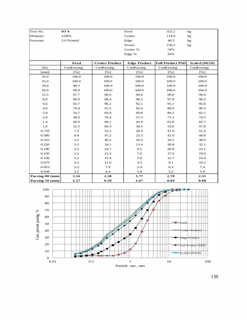
130
Test No. IO 4 Feed 322.2 kg
Moisture 4.00% Center 114.9 kg
Pressure 2.0 N/mm2 Edge 40.2 kg
Waste 158.2 kg
Center % 74%
Edge % 26%
Feed Center Product Edge Product Full Product PSD Scaled (90/10)
Size Cum. Passing Cum. Passing Cum. Passing Cum. Passing Cum. Passing
[mm] [%] [%] [%] [%] [%]
32.0 100.0 100.0 100.0 100.0 100.0
25.0 100.0 100.0 100.0 100.0 100.0
19.0 99.5 100.0 100.0 100.0 100.0
16.0 99.0 100.0 100.0 100.0 100.0
12.5 97.7 99.9 99.8 99.9 99.9
8.0 90.9 98.4 96.3 97.9 98.2
5.6 83.7 96.2 92.1 95.1 95.8
4.0 70.4 91.2 82.4 88.9 90.3
2.8 54.7 83.9 69.8 80.2 82.5
2.0 38.4 76.4 57.3 71.5 74.5
1.4 20.9 68.1 43.9 61.8 65.7
1.0 12.5 60.3 34.5 53.6 57.8
0.710 7.2 53.5 28.4 47.0 51.0
0.500 4.8 47.2 23.3 41.0 44.8
0.355 3.2 40.2 18.5 34.5 38.0
0.250 3.2 34.1 13.4 28.8 32.1
0.180 3.2 24.7 9.5 20.8 23.2
0.150 3.2 21.3 7.0 17.6 19.9
0.106 3.2 15.4 5.0 12.7 14.4
0.075 3.2 11.0 3.5 9.1 10.3
0.053 3.2 7.9 2.4 6.5 7.4
0.038 3.2 6.4 1.8 5.2 5.9
Passing 80 (mm) 5.16 2.38 3.77 2.78 2.55
Passing 50 (mm) 2.57 0.59 1.67 0.84 0.68
0
10
20
30
40
50
60
70
80
90
100
0.01 0.1 1 10 100
Cum
. per
cent
pas
sing,
%
Particle size, mm
Feed
Center Product
Edge Product
Full Product PSD
Scaled (90/10)
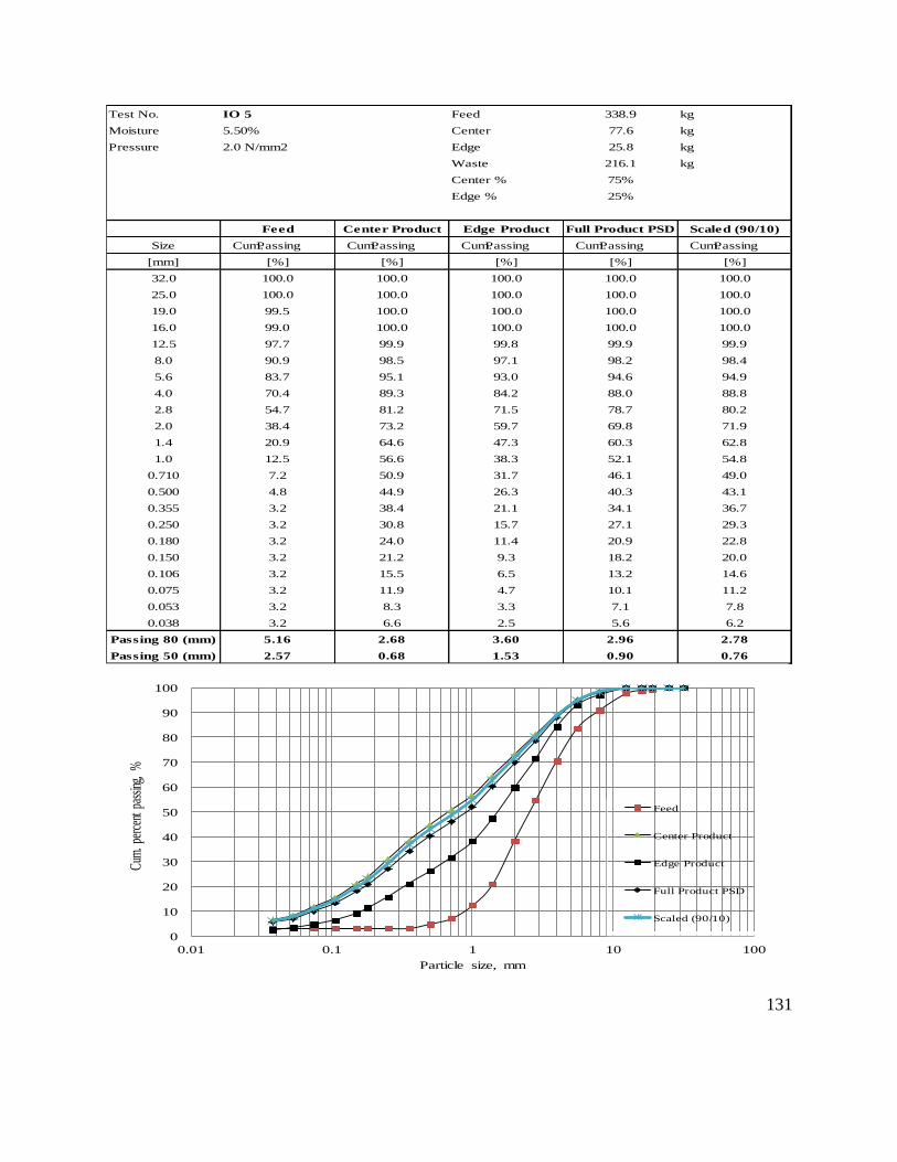
131
Test No. IO 5 Feed 338.9 kg
Moisture 5.50% Center 77.6 kg
Pressure 2.0 N/mm2 Edge 25.8 kg
Waste 216.1 kg
Center % 75%
Edge % 25%
Feed Center Product Edge Product Full Product PSD Scaled (90/10)
Size Cum. Passing Cum. Passing Cum. Passing Cum. Passing Cum. Passing
[mm] [%] [%] [%] [%] [%]
32.0 100.0 100.0 100.0 100.0 100.0
25.0 100.0 100.0 100.0 100.0 100.0
19.0 99.5 100.0 100.0 100.0 100.0
16.0 99.0 100.0 100.0 100.0 100.0
12.5 97.7 99.9 99.8 99.9 99.9
8.0 90.9 98.5 97.1 98.2 98.4
5.6 83.7 95.1 93.0 94.6 94.9
4.0 70.4 89.3 84.2 88.0 88.8
2.8 54.7 81.2 71.5 78.7 80.2
2.0 38.4 73.2 59.7 69.8 71.9
1.4 20.9 64.6 47.3 60.3 62.8
1.0 12.5 56.6 38.3 52.1 54.8
0.710 7.2 50.9 31.7 46.1 49.0
0.500 4.8 44.9 26.3 40.3 43.1
0.355 3.2 38.4 21.1 34.1 36.7
0.250 3.2 30.8 15.7 27.1 29.3
0.180 3.2 24.0 11.4 20.9 22.8
0.150 3.2 21.2 9.3 18.2 20.0
0.106 3.2 15.5 6.5 13.2 14.6
0.075 3.2 11.9 4.7 10.1 11.2
0.053 3.2 8.3 3.3 7.1 7.8
0.038 3.2 6.6 2.5 5.6 6.2
Passing 80 (mm) 5.16 2.68 3.60 2.96 2.78
Passing 50 (mm) 2.57 0.68 1.53 0.90 0.76
0
10
20
30
40
50
60
70
80
90
100
0.01 0.1 1 10 100
Cum
. per
cent
pas
sing,
%
Particle size, mm
Feed
Center Product
Edge Product
Full Product PSD
Scaled (90/10)
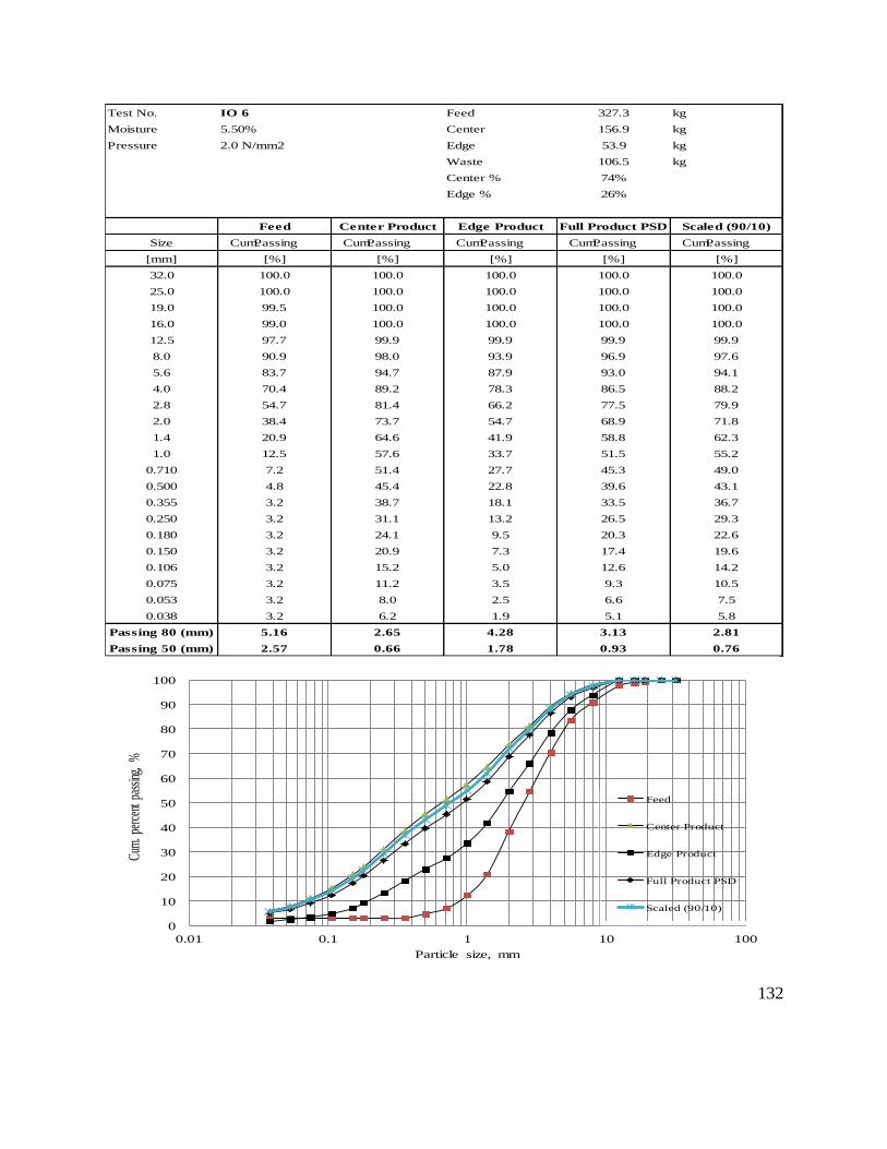
132
Test No. IO 6 Feed 327.3 kg
Moisture 5.50% Center 156.9 kg
Pressure 2.0 N/mm2 Edge 53.9 kg
Waste 106.5 kg
Center % 74%
Edge % 26%
Feed Center Product Edge Product Full Product PSD Scaled (90/10)
Size Cum. Passing Cum. Passing Cum. Passing Cum. Passing Cum. Passing
[mm] [%] [%] [%] [%] [%]
32.0 100.0 100.0 100.0 100.0 100.0
25.0 100.0 100.0 100.0 100.0 100.0
19.0 99.5 100.0 100.0 100.0 100.0
16.0 99.0 100.0 100.0 100.0 100.0
12.5 97.7 99.9 99.9 99.9 99.9
8.0 90.9 98.0 93.9 96.9 97.6
5.6 83.7 94.7 87.9 93.0 94.1
4.0 70.4 89.2 78.3 86.5 88.2
2.8 54.7 81.4 66.2 77.5 79.9
2.0 38.4 73.7 54.7 68.9 71.8
1.4 20.9 64.6 41.9 58.8 62.3
1.0 12.5 57.6 33.7 51.5 55.2
0.710 7.2 51.4 27.7 45.3 49.0
0.500 4.8 45.4 22.8 39.6 43.1
0.355 3.2 38.7 18.1 33.5 36.7
0.250 3.2 31.1 13.2 26.5 29.3
0.180 3.2 24.1 9.5 20.3 22.6
0.150 3.2 20.9 7.3 17.4 19.6
0.106 3.2 15.2 5.0 12.6 14.2
0.075 3.2 11.2 3.5 9.3 10.5
0.053 3.2 8.0 2.5 6.6 7.5
0.038 3.2 6.2 1.9 5.1 5.8
Passing 80 (mm) 5.16 2.65 4.28 3.13 2.81
Passing 50 (mm) 2.57 0.66 1.78 0.93 0.76
0
10
20
30
40
50
60
70
80
90
100
0.01 0.1 1 10 100
Cum
. per
cent
pas
sing,
%
Particle size, mm
Feed
Center Product
Edge Product
Full Product PSD
Scaled (90/10)

133
Test No. CO 1 Feed 260.8 kg
Moisture 1.48% Center 100.4 kg
Pressure 5.0 N/mm2 Edge 36.8 kg
Waste 122.5 kg
Center % 73%
Edge % 27%
Feed Center Product Edge Product Full Product PSD Scaled (90/10)
Size Cum. Passing Cum. Passing Cum. Passing Cum. Passing Cum. Passing
[mm] [%] [%] [%] [%] [%]
32.0 100.0 100.0 100.0 100.0 100.0
25.0 100.0 100.0 100.0 100.0 100.0
19.0 99.5 100.0 99.9 100.0 100.0
16.0 99.0 99.9 99.1 99.6 99.8
12.5 97.7 98.5 93.6 97.2 98.0
8.0 90.9 91.8 75.3 87.4 90.1
5.6 83.7 85.7 63.5 79.7 83.5
4.0 70.4 79.3 54.4 72.6 76.8
2.8 54.7 71.6 45.6 64.6 69.0
2.0 38.4 64.4 39.2 57.6 61.8
1.4 20.9 57.2 32.9 50.7 54.8
1.0 12.5 51.1 28.2 45.0 48.8
0.710 7.2 44.6 24.3 39.1 42.5
0.500 4.8 38.2 20.6 33.5 36.4
0.355 3.2 32.7 17.5 28.6 31.1
0.250 3.2 27.3 14.6 23.9 26.0
0.180 3.2 22.2 12.0 19.5 21.2
0.125 3.2 16.4 9.0 14.4 15.7
0.090 3.2 13.1 7.1 11.5 12.5
0.063 3.2 8.7 4.9 7.7 8.4
0.045 3.2 6.5 3.8 5.8 6.2
Passing 80 (mm) 5.16 4.18 9.16 5.68 4.77
Passing 50 (mm) 2.57 0.95 3.40 1.35 1.08
0
10
20
30
40
50
60
70
80
90
100
0.01 0.1 1 10 100
Cum
. per
cent
pas
sing,
%
Particle size, mm
Feed
Center Product
Edge Product
Full Product PSD
Scaled (90/10)

134
Test No. CO 2 Feed 262.4 kg
Moisture 1.48% Center 97.4 kg
Pressure 4.0 N/mm2 Edge 41.5 kg
Waste 118.5 kg
Center % 70%
Edge % 30%
Feed Center Product Edge Product Full Product PSD Scaled (90/10)
Size Cum. Passing Cum. Passing Cum. Passing Cum. Passing Cum. Passing
[mm] [%] [%] [%] [%] [%]
32.0 100.0 100.0 100.0 100.0 100.0
25.0 100.0 100.0 100.0 100.0 100.0
19.0 99.5 100.0 100.0 100.0 100.0
16.0 99.0 99.9 98.7 99.6 99.8
12.5 97.7 98.0 92.8 96.4 97.4
8.0 90.9 90.5 72.2 85.0 88.7
5.6 83.7 83.4 60.9 76.7 81.1
4.0 70.4 76.2 52.1 69.0 73.8
2.8 54.7 68.0 43.5 60.7 65.6
2.0 38.4 60.3 37.2 53.4 58.0
1.4 20.9 53.0 31.2 46.5 50.9
1.0 12.5 46.1 26.9 40.3 44.2
0.710 7.2 40.0 22.9 34.9 38.3
0.500 4.8 34.4 19.6 30.0 32.9
0.355 3.2 29.4 16.8 25.7 28.2
0.250 3.2 24.4 14.0 21.3 23.4
0.180 3.2 20.0 11.5 17.5 19.2
0.125 3.2 14.9 8.6 13.0 14.3
0.090 3.2 10.9 6.4 9.6 10.5
0.063 3.2 7.3 4.3 6.4 7.0
0.045 3.2 4.8 3.2 4.3 4.6
Passing 80 (mm) 5.16 4.85 9.70 6.55 5.35
Passing 50 (mm) 2.57 1.23 3.71 1.70 1.35
0
10
20
30
40
50
60
70
80
90
100
0.01 0.1 1 10 100
Cum
. per
cent
pas
sing,
%
Particle size, mm
Feed
Center Product
Edge Product
Full Product PSD
Scaled (90/10)

135
Test No. CO 3 Feed 261.1 kg
Moisture 1.48% Center 99.8 kg
Pressure 3.0 N/mm2 Edge 42.2 kg
Waste 115 kg
Center % 70%
Edge % 30%
Feed Center Product Edge Product Full Product PSD Scaled (90/10)
Size Cum. Passing Cum. Passing Cum. Passing Cum. Passing Cum. Passing
[mm] [%] [%] [%] [%] [%]
32.0 100.0 100.0 100.0 100.0 100.0
25.0 100.0 100.0 100.0 100.0 100.0
19.0 99.5 100.0 99.9 100.0 100.0
16.0 99.0 99.5 98.5 99.2 99.4
12.5 97.7 97.0 91.4 95.4 96.5
8.0 90.9 87.1 70.2 82.1 85.4
5.6 83.7 79.0 56.3 72.2 76.7
4.0 70.4 71.5 47.4 64.3 69.1
2.8 54.7 63.1 39.3 56.1 60.7
2.0 38.4 55.7 33.3 49.1 53.5
1.4 20.9 48.2 27.9 42.2 46.2
1.0 12.5 41.7 23.7 36.4 39.9
0.710 7.2 35.9 20.2 31.2 34.3
0.500 4.8 30.8 17.1 26.7 29.4
0.355 3.2 26.0 14.6 22.6 24.9
0.250 3.2 21.4 12.2 18.7 20.5
0.180 3.2 17.6 9.8 15.3 16.9
0.125 3.2 13.4 7.2 11.6 12.8
0.090 3.2 10.3 5.3 8.8 9.8
0.063 3.2 7.5 3.4 6.3 7.1
0.045 3.2 5.7 2.6 4.8 5.4
Passing 80 (mm) 5.16 5.90 10.08 7.49 6.50
Passing 50 (mm) 2.57 1.54 4.46 2.11 1.72
0
10
20
30
40
50
60
70
80
90
100
0.01 0.1 1 10 100
Cum
. per
cent
pas
sing,
%
Particle size, mm
Feed
Center Product
Edge Product
Full Product PSD
Scaled (90/10)
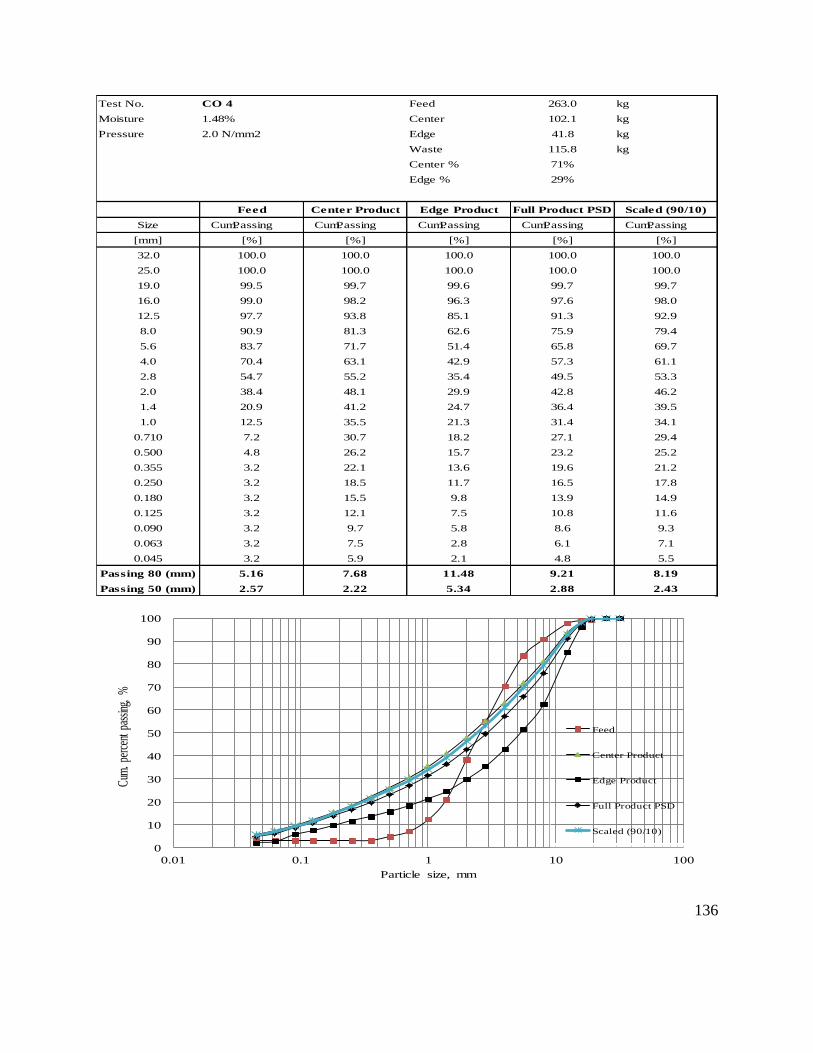
136
Test No. CO 4 Feed 263.0 kg
Moisture 1.48% Center 102.1 kg
Pressure 2.0 N/mm2 Edge 41.8 kg
Waste 115.8 kg
Center % 71%
Edge % 29%
Feed Center Product Edge Product Full Product PSD Scaled (90/10)
Size Cum. Passing Cum. Passing Cum. Passing Cum. Passing Cum. Passing
[mm] [%] [%] [%] [%] [%]
32.0 100.0 100.0 100.0 100.0 100.0
25.0 100.0 100.0 100.0 100.0 100.0
19.0 99.5 99.7 99.6 99.7 99.7
16.0 99.0 98.2 96.3 97.6 98.0
12.5 97.7 93.8 85.1 91.3 92.9
8.0 90.9 81.3 62.6 75.9 79.4
5.6 83.7 71.7 51.4 65.8 69.7
4.0 70.4 63.1 42.9 57.3 61.1
2.8 54.7 55.2 35.4 49.5 53.3
2.0 38.4 48.1 29.9 42.8 46.2
1.4 20.9 41.2 24.7 36.4 39.5
1.0 12.5 35.5 21.3 31.4 34.1
0.710 7.2 30.7 18.2 27.1 29.4
0.500 4.8 26.2 15.7 23.2 25.2
0.355 3.2 22.1 13.6 19.6 21.2
0.250 3.2 18.5 11.7 16.5 17.8
0.180 3.2 15.5 9.8 13.9 14.9
0.125 3.2 12.1 7.5 10.8 11.6
0.090 3.2 9.7 5.8 8.6 9.3
0.063 3.2 7.5 2.8 6.1 7.1
0.045 3.2 5.9 2.1 4.8 5.5
Passing 80 (mm) 5.16 7.68 11.48 9.21 8.19
Passing 50 (mm) 2.57 2.22 5.34 2.88 2.43
0
10
20
30
40
50
60
70
80
90
100
0.01 0.1 1 10 100
Cum
. per
cent
pas
sing,
%
Particle size, mm
Feed
Center Product
Edge Product
Full Product PSD
Scaled (90/10)

137
Appendix B - Single particle compression tests
B.1 Iron ore
Force (N) Mass (g)
1 1916.9 2.42
2 2175.3 2.73
3 1499.1 2.60
4 1750.6 2.48
5 1757.8 2.64
6 482.5 2.34
7 2403.2 2.05
8 1302.9 2.88
9 2710.8 2.24
10 2299.1 2.30
11 1843.0 1.82
12 2700.7 2.48
13 1991.7 2.50
14 972.7 2.32
15 1386.1 1.84
16 1689.7 2.26
17 1374.6 3.48
18 1348.5 2.86
19 1402.4 1.93
20 1736.8 2.20
Average 1737.2 2.42
Std. Dev. 541.3 0.38
Error % 31.2 15.83
Iron ore (-11.20 + 9.50 mm)
500
1000
1500
2000
2500
3000
0 5 10 15 20
Fo
rce
, N
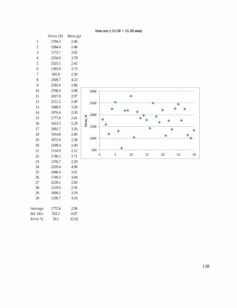
138
Force (N) Mass (g)
1 1794.3 2.96
2 1584.4 2.48
3 1172.7 3.62
4 2254.9 3.78
5 2525.1 2.42
6 1302.9 3.73
7 565.9 2.30
8 2169.7 4.23
9 2185.9 2.86
10 2796.9 2.98
11 1027.8 2.97
12 2112.2 2.40
13 1848.9 3.30
14 1974.4 2.50
15 1777.8 2.61
16 1423.3 2.29
17 2491.7 3.26
18 1914.8 2.60
19 1672.0 2.28
20 2199.4 2.40
21 1110.9 2.12
22 1740.2 2.71
23 1376.7 2.29
24 2259.4 4.98
25 2446.4 3.01
26 1749.3 3.04
27 2239.1 2.83
28 1129.6 2.56
29 1000.2 3.19
30 1330.7 4.16
Average 1772.6 2.96
Std. Dev. 533.2 0.67
Error % 30.1 22.62
Iron ore (-12.50 + 11.20 mm)
500
1000
1500
2000
2500
3000
0 5 10 15 20 25 30
Forc
e,
N

139
Force (N) Mass (g)
1 1599.7 7.11
2 1848.2 3.76
3 230.4 4.51
4 1508.1 7.56
5 4157.2 6.22
6 2429.4 8.39
7 4275.5 8.74
8 4101.2 8.41
9 2187.3 4.04
10 1775.7 4.38
11 2350.8 4.86
12 2067.0 5.26
13 2089.7 3.60
14 1323.9 4.62
15 3769.0 5.22
16 1245.2 5.43
17 3734.5 5.32
18 1767.5 4.93
19 3230.5 3.62
20 2250.7 4.30
21 2772.4 4.04
22 3596.4 4.80
23 3122.9 4.46
24 2233.8 7.51
25 3210.3 3.90
26 2577.0 3.75
27 2213.8 4.20
28 2100.8 5.43
29 919.0 4.32
30 1315.2 8.74
Average 2400.1 5.38
Std. Dev. 1002.6 1.62
Error % 41.8 30.13
Iron ore (-16.00 + 12.50 mm)
1000
1500
2000
2500
3000
3500
4000
4500
0 5 10 15 20 25 30
Forc
e,
N

140
Force (N) Mass (g)
1 3325.5 9.32
2 4928.8 10.74
3 2267.9 11.13
4 3701.5 10.17
5 5037.0 7.35
6 3704.7 12.28
7 3310.9 6.61
8 6347.9 7.91
9 1625.3 10.00
10 1604.1 7.59
11 2516.0 6.83
12 4511.9 16.77
13 2359.1 8.83
14 1935.6 8.23
15 1342.6 8.20
16 4877.4 10.71
17 3212.7 5.75
18 2595.2 6.21
19 3398.5 14.54
20 3949.8 6.35
Average 3327.6 9.28
Std. Dev. 1305.8 2.79
Error % 39.2 30.13
Iron ore (-19.00 + 16.00 mm)
1000
2000
3000
4000
5000
6000
7000
0 5 10 15 20
Forc
e,
N

141
Force (N) Mass (g)
1 7136.1 16.08
2 7367.2 25.71
3 2427.6 13.46
4 6014.9 11.05
5 4973.7 11.54
6 4395.2 11.07
7 6876.1 18.03
8 1806.4 18.69
9 4667.6 16.84
10 1759.9 11.41
Average 4742.5 15.39
Std. Dev. 2045.6 4.46
Error % 43.1 28.98
Iron ore (-25.40 + 19.00 mm)
4000
4500
5000
5500
6000
6500
7000
7500
8000
0 2 4 6 8 10
Fo
rce
, N
Force (N) Mass (g)
Force Mass
1 4642.1 49.71
2 6040.3 51.23
3 6210.3 44.81
4 5489.5 29.27
5 4415.6 26.20
Average 5359.6 40.24
Std. Dev. 722.5 10.48
Error % 13.5 26.03
Iron ore (-32.00 + 25.40 mm)
4000
5000
6000
7000
0 1 2 3 4 5
Fo
rce
, N

142
B.2 Copper ore
Force (N) Mass (g)
1 1542.1 2.66
2 1041.0 2.35
3 1723.9 1.89
4 1823.6 2.64
5 1479.2 1.70
6 1236.9 1.65
7 1604.5 1.78
8 1817.9 1.58
9 1360.1 2.63
10 2623.7 2.32
11 791.5 2.16
12 1271.6 2.61
13 1837.0 1.80
14 2575.9 2.26
15 2102.1 2.13
16 1820.2 2.03
17 1575.6 2.37
18 1767.4 1.78
19 2571.0 2.27
20 2385.2 3.24
21 2213.3 2.26
22 2127.1 2.56
23 1466.9 2.12
24 1782.6 1.79
25 1678.9 1.78
26 2528.8 2.76
27 1396.3 2.70
28 2283.2 2.40
29 1396.7 2.19
30 2622.9 2.16
Average 1814.9 2.22
Std. Dev. 487.3 0.39
Error % 26.8 17.60
Copper ore (-11.20 + 9.50 mm)
500
1000
1500
2000
2500
3000
0 5 10 15 20 25 30
Forc
e,
N

143
Force (N) Mass (g)
1 2505.7 4.04
2 2685.5 3.71
3 2487.6 3.78
4 2286.7 3.41
5 3483.1 3.26
6 1971.4 3.05
7 2411.7 3.77
8 2469.3 3.05
9 3224.2 3.81
10 1706.7 3.07
11 2012.2 2.48
12 2740.9 3.25
13 1984.7 2.44
14 1874.7 3.71
15 2613.3 4.01
16 2107.6 2.87
17 1966.1 2.39
18 1629.0 3.74
19 2337.2 2.69
20 3070.9 2.99
21 1475.1 2.98
22 2406.4 2.68
23 2212.1 2.38
24 2491.9 2.70
25 1500.1 2.30
26 1758.0 2.64
27 1917.5 2.10
28 1511.5 3.28
29 2029.2 2.53
30 2378.2 2.90
Average 2241.6 3.07
Std. Dev. 491.5 0.55
Error % 21.9 17.93
Copper ore (-12.50 + 11.20 mm)
1000
1500
2000
2500
3000
3500
0 5 10 15 20 25 30
Forc
e,
N

144
Force (N) Mass (g)
1 3314.0 5.50
2 4772.7 4.91
3 4898.8 6.26
4 3843.8 6.58
5 3081.8 5.74
6 4348.4 4.97
7 3720.1 4.12
8 3706.6 4.79
9 2734.2 6.98
10 2151.0 5.33
11 2938.2 3.66
12 2330.6 4.40
13 3678.1 6.35
14 2060.7 4.12
15 2811.5 4.70
16 2572.2 4.79
17 4011.2 4.53
18 3188.8 5.31
19 4249.3 6.91
20 3081.1 5.60
21 3667.7 5.54
22 3044.4 4.31
23 3028.3 4.14
24 2664.9 4.45
25 3611.1 5.70
26 3041.2 5.53
27 2242.6 5.23
28 4862.3 7.04
29 3659.1 8.20
30 3292.5 3.74
Average 3353.6 5.31
Std. Dev. 765.5 1.07
Error % 22.8 20.21
Copper ore (-16.00 + 12.50 mm)
2000
2500
3000
3500
4000
4500
5000
0 5 10 15 20 25 30
Forc
e,
N
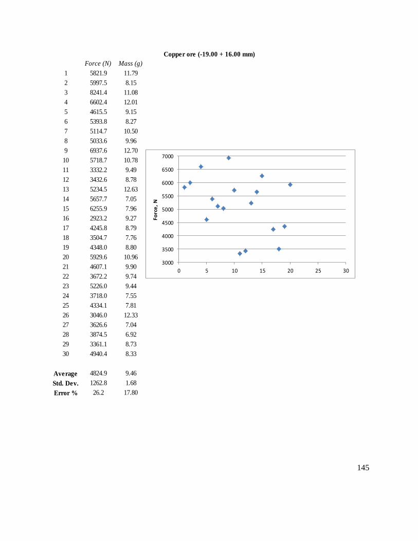
145
Force (N) Mass (g)
1 5821.9 11.79
2 5997.5 8.15
3 8241.4 11.08
4 6602.4 12.01
5 4615.5 9.15
6 5393.8 8.27
7 5114.7 10.50
8 5033.6 9.96
9 6937.6 12.70
10 5718.7 10.78
11 3332.2 9.49
12 3432.6 8.78
13 5234.5 12.63
14 5657.7 7.05
15 6255.9 7.96
16 2923.2 9.27
17 4245.8 8.79
18 3504.7 7.76
19 4348.0 8.80
20 5929.6 10.96
21 4607.1 9.90
22 3672.2 9.74
23 5226.0 9.44
24 3718.0 7.55
25 4334.1 7.81
26 3046.0 12.33
27 3626.6 7.04
28 3874.5 6.92
29 3361.1 8.73
30 4940.4 8.33
Average 4824.9 9.46
Std. Dev. 1262.8 1.68
Error % 26.2 17.80
Copper ore (-19.00 + 16.00 mm)
3000
3500
4000
4500
5000
5500
6000
6500
7000
0 5 10 15 20 25 30
Forc
e,
N

146
Force (N) Mass (g)
1 5994.8 18.74
2 10381.7 19.17
3 5354.4 20.71
4 4374.6 15.54
5 8734.0 28.20
6 11040.1 24.88
7 5684.8 30.13
8 4766.0 22.14
9 6033.5 21.61
10 6865.0 21.60
11 7821.2 20.46
12 5997.6 22.76
13 7800.5 19.92
14 2743.0 17.51
15 9731.0 17.17
16 3182.3 17.82
17 12872.4 22.43
18 5896.7 22.48
19 4385.4 14.29
20 4399.2 15.11
21 3204.4 17.53
23 5667.7 15.80
24 8899.9 15.07
25 3394.9 20.30
26 3130.2 13.65
27 7228.6 15.06
28 8310.9 16.60
29 2673.1 13.34
30 5753.5 14.96
30 9582.2 17.52
Average 6396.8 19.08
Std. Dev. 2622.9 4.07
Error % 41.0 21.32
Copper ore (-25.40 + 19.00 mm)
3000
4000
5000
6000
7000
8000
9000
10000
11000
0 5 10 15 20 25 30
Forc
e,
N

147
Force (N) Mass (g)
1 3855.247 27.913
2 6239.644 34.990
3 9433.032 35.710
4 8945.170 33.947
5 7001.174 39.050
6 5639.351 33.779
7 5028.864 36.860
8 7577.074 33.570
9 4542.054 27.730
10 7921.655 30.448
11 8538.829 32.639
12 4383.090 27.990
13 7608.987 32.360
14 5876.109 35.128
15 8650.760 43.635
Average 6749.4 33.72
Std. Dev. 1746.7 4.17
Error % 25.9 12.36
Copper ore (-32.00 + 25.40 mm)
3000
4000
5000
6000
7000
8000
9000
10000
11000
0 2 4 6 8 10 12 14
Fo
rce
, N