Predicting Financial Distress and the Performance of DistressedStocks

(Article begins on next page)

The Harvard community has made this article openly available.Please share how this access benefits you. Your story matters.

Citation Campbell, John Y., Jens Dietrich Hilscher, and Jan Szilagyi. 2011.Predicting financial distress and the performance of distressedstocks. Journal of Investment Management 9(2): 14-34.

Published Version https://www.joim.com/abstract.asp?IsArticleArchived=1&ArtID=401

Accessed July 14, 2018 1:45:03 PM EDT

Citable Link http://nrs.harvard.edu/urn-3:HUL.InstRepos:9887619

Terms of Use This article was downloaded from Harvard University's DASHrepository, and is made available under the terms and conditionsapplicable to Open Access Policy Articles, as set forth athttp://nrs.harvard.edu/urn-3:HUL.InstRepos:dash.current.terms-of-use#OAP

Predicting Financial Distress and the Performanceof Distressed Stocks

John Y. Campbell, Jens Hilscher, and Jan Szilagyi1

January 2010

1John Y. Campbell, Department of Economics, Littauer Center 213, Harvard University, Cam-bridge MA 02138, USA, and NBER. Tel 617-496-6448, email john_campbell@harvard.edu. JensHilscher, International Business School, Brandeis University, 415 South Street, Waltham MA 02453,USA. Phone 781-736-2261, email hilscher@brandeis.edu. Jan Szilagyi, Duquesne Capital Manage-ment LLC, 40 West 57th Street, 25th Floor, New York NY 10019, USA. Phone 212-830-6665, emailjan@duquesne.com. The views expressed in this paper are those of the authors and do not necessar-ily represent the views of the authors�employers. This material is based upon work supported bythe National Science Foundation under Grant No. 0214061 to Campbell. We would like to thankRobert Jarrow and Don van Deventer of Kamakura Risk Information Services (KRIS) for providingus with data on corporate failures.

Abstract

In this paper we consider the measurement and pricing of distress risk. We presenta model of corporate failure in which accounting and market-based measures forecastthe likelihood of future �nancial distress. Our best model is more accurate thanleading alternative measures of corporate failure risk. We then use our measure of�nancial distress to examine the performance of distressed stocks from 1981 to 2008.We �nd that distressed stocks have highly variable returns and high market betas andthat they tend to underperform safe stocks by more at times of high market volatilityand risk aversion. However, investors in distressed stocks have not been rewardedfor bearing these risks. Instead, distressed stocks have had very low returns, bothrelative to the market and after adjusting for their high risk. The underperformanceof distressed stocks is present in all size and value quintiles. It is lower for stockswith low analyst coverage and institutional holdings, which suggests that informationor arbitrage-related frictions may be partly responsible for the underperformance ofdistressed stocks.

1 Introduction

Interest in the pricing of �nancially distressed �rms is widespread. Chan and Chen(1991) describe marginal and distressed �rms as follows: �They have lost marketvalue because of poor performance, they are ine¢ cient producers, and they are likelyto have high �nancial leverage and cash �ow problems. They are marginal in thesense that their prices tend to be more sensitive to changes in the economy, and theyare less likely to survive adverse economic conditions.� Asset pricing theory suggeststhat investors will demand a premium for holding such stocks. It is an empiricalquestion whether or not investors are indeed rewarded for bearing such risk.

We investigate the pricing of �nancially distressed stocks in two steps: First, wepresent a model predicting �nancial distress. Second, we consider the historicalperformance of investing in distressed stock portfolios.

Our proposed measure of �nancial distress is the probability of failure. FollowingShumway (2001) we predict failure in a hazard model using explanatory variablesconstructed from observable accounting and market-based measures. This approachis related to an earlier literature pioneered by Beaver (1966) and Altman (1968) whointroduced Z-score as a measure of bankruptcy risk, and has recently been used byBeaver, McNichols, and Rhie (2005).

We classify a �rm as more distressed if it is more likely to �le for bankruptcy underChapter 7 or Chapter 11, de-list for performance related reasons, or receive a D ratingfrom a rating agency. This expanded measure of failure (relative to measuring onlybankruptcy �lings) allows us to capture at least some instances in which �rms fail butreach an agreement with creditors before an actual bankruptcy �ling (Gilson, John,and Lang 1990, Gilson 1997). Our data set is monthly and includes more than 2million �rm-months and close to 1,750 failure events.

We predict failure over the next month (similar to Chava and Jarrow (2004)).However, in addition we also consider the probability of failure for longer horizons.After all, an investor will certainly care not only about imminent failure, but ratherwill want to get a sense well in advance which are the �rms that are most likely tofail. Although probably quite accurate, it may not be useful to predict a heart attackwith a person clutching their hand to their chest.

Firms that are distressed have the characteristics we would expect: they have re-

1

cently made losses, have high leverage, their stock returns have been low and volatile,and they have low levels of cash holdings. Our best model, which makes severalchanges relative to Shumway (2001) and Chava and Jarrow (2004), improves forecastaccuracy by 16% when compared to these models. It also outperforms another lead-ing alternative ��distance-to-default��a measure based on the famous Merton (1974)model of risky corporate debt and popularized by Moody�s KMV (see, for example,Crosbie and Bohn(2001)). Relative to distance-to-default our model almost doublesforecast accuracy.

We next investigate the performance of distressed stocks using our best modelto measure �nancial distress. Portfolios of distressed stocks have very high levelsof volatility and high market betas, which means that they are risky and shouldcommand a high risk premium. However, their returns from 1981 to 2008 have beenlow: distressed stocks have signi�cantly underperformed the S&P500. A portfoliogoing long safe stocks and shorting distressed stocks has been a highly pro�tablestrategy and has a signi�cantly higher average return and Sharpe ratio than theS&P500.

The underperformance of distressed stocks is puzzling given that investors seemto realize that distressed stocks are risky: The high market betas of distressed stocksimply that the market perceives distressed stocks as being more sensitive to overallmarket conditions. Furthermore, we �nd that distressed stocks underperform moreseverely at times of increases in market volatility, as measured by the VIX, the impliedvolatility of S&P500 index options. In the last four months of 2008 a strategy oflong safe, short distressed stocks earned a return of 59%, while the return for all of2008 was 145%.

Even if the average investor does not react, such high performance levels shouldattract signi�cant arbitrage capital and over time we should see declining pro�ts tothis strategy. One reason why we have not observed this could be that it is di¢ cultto obtain information about the health of distressed stocks and that they may bedi¢ cult to short sell. Due to these constraints arbitrage activity could be limited.Consistent with this hypothesis we �nd that the distress e¤ect is more concentratedin stocks with low analyst coverage and in stocks with low levels of institutionalholdings, which has been proposed as a proxy for the ability to short such stocks.

The remainder of the paper is organized as follows. After a brief review of theexisting literature, Section 2 discusses our data and the construction of our explana-tory variables. Section 3 presents our model of failure prediction. We investigate the

2

ability of our variables to predict failure at di¤erent horizons and compare the fore-cast accuracy of our best model to leading alternatives. We also consider the abilityof our model to predict changes in the aggregate failure rate over time. Section 4focuses on the performance of distressed stock portfolios. We document performanceover time and consider performance across size and value quintiles, as well as for �rmswith higher information and arbitrage-related frictions. Section 5 concludes.

1.1 Related literature

There are several di¤erent approaches to predicting bankruptcy. Early studies fo-cused entirely on accounting ratios and often compared �nancial ratios in a group ofnon-bankrupt �rms to a group of bankrupt �rms, e.g. Altman�s (1968) Z-score. Thesubsequent literature introduced market-based variables and adopted more suitablestatistical techniques to model probability of bankruptcy. Shumway (2001) discussesthis line of research and points out the shortcomings of the early studies. Our pa-per adds to this line of work by developing the variables used by Shumway (2001)further and adding additional variables that lead to a large increase in the model�sexplanatory power.

Other studies have instead focused on using Merton (1974) as the basis for model-ing and have chosen distance-to-default as the main variable to predict future bank-ruptcy. Examples include Hillegeist et al. (2004), Vassalou and Xing (2004), andDu¢ e et al. (2007). We show that using a larger set of explanatory has signi�cantlyhigher forecasting ability, a fact also pointed out by Bharath and Shumway (2008).

Another possibility is to use credit ratings as a summary measure of the risk offuture bankruptcy. Hilscher and Wilson (2009) �nd that using the model describedbelow has much higher forecast accuracy than credit ratings.

2 Constructing measures of �nancial distress

Our measure of �nancial distress is the probability of failure. We de�ne failure to bethe �rst of the following events: chapter 7 or chapter 11 bankruptcy �ling, de-listingdue to performance related reasons, and a default or selective default rating by arating agency. We use monthly failure event data that runs from January 1963 to

3

December 2008. Our data on failures was provided by Kamakura Risk InformationServices (KRIS) and represents an updated version of the data in Campbell, Hilscher,and Szilagyi (2008), who use data up to December 2003.

We use accounting and market-based measures to forecast failure. Taking themodels used in Shumway (2001) and Chava and Jarrow (2004) as the starting pointwe construct the following eight measures of �nancial distress, three accounting-basedmeasures and �ve market-based measures. We construct all our measures usingquarterly and annual accounting data from COMPUSTAT and daily and monthlydata from CRSP.

1. We measure pro�tability as the ratio of net income (losses) over the previousquarter to the market value of total assets (NIMTA). We �nd that the marketvalue of total assets, the sum of book value of total liabilities and market equity,is a more accurate measure of assets than book value of total assets, a measureused to scale income in previous studies. Scaling by market value of assetsgives a potentially more timely and accurate picture of the asset value of the�rm. Market equity capitalization is available in real time and re�ects recentnews to the �rm. Furthermore, it also allows for a more accurate valuationof assets, e.g. growth opportunities, intangibles, departure from replacementvalue, and may also re�ect the �nancing capacity of the �rm both in terms ofequity issuance as well as its ability to secure short-term �nancing.

2. Our measure of leverage is total liabilities divided by market total assets (TLMTA).Similar to pro�tability, we �nd that this measure more accurately re�ects dis-tress than when scaling by book value of total assets.

3. We measure short-term liquidity using cash holdings scaled by market totalassets (CASHMTA). If a �rm runs out of cash and cannot secure �nancingit will fail, even if its value of assets is larger than the level of its liabilities.

4. We add the �rm�s equity return (EXRET ) which is the stock�s excess returnrelative to the S&P 500 index return. We expect �rms close to bankruptcy andfailure to have negative returns.

5. Volatility (SIGMA) is a measure of the stock�s standard deviation over theprevious three months. Not surprisingly, distressed �rms�stocks returns arehighly volatile.

4

6. Relative size (RSIZE) is the �rm�s equity capitalization relative to the S&P500index, which we measure by taking the log of the ratio. We expect, ceterisparibus, smaller �rms to have less of an ability to secure temporary �nancingto prevent failure.

7. We calculate the �rm�s ratio of market equity to book equity (MB). Market-to-book may capture over-valuation of distressed �rms that have recently ex-perienced heavy losses. It may also be important in modeling default since itmight enter as an adjustment factor to our three accounting measures that arescaled by market equity.

8. We add the log of the stock price, which we cap at $15 (PRICE). Distressed�rms often have very low prices, a re�ection of their decline in equity value.If �rms are slow or reluctant to implement reverse stock splits this measurewill be related to failure. Variation above $15 does not seem to a¤ect failureprobability and so the measure is capped at that level.

All of our measures are lagged so that they are observable at the beginning of themonth over which we measure whether or not the �rm fails. The three accountingmeasures are based on quarterly data and we assume that it is available two monthsafter the end of the accounting quarter. Market data is measured at the end of theprevious month. This way we ensure that the failure prediction we propose can beimplemented in real time and that the investment returns that we discuss in Section4 can be constructed using available data.

To control for outliers we winsorize the variables at the 5th and 95th percentile oftheir distributions. This means that we replace any value below the 5th percentilewith the 5th percentile value and replace values above the 95th percentile with the95th percentile value. The appendix of the paper describes the variable constructionin more detail.

2.1 Summary statistics

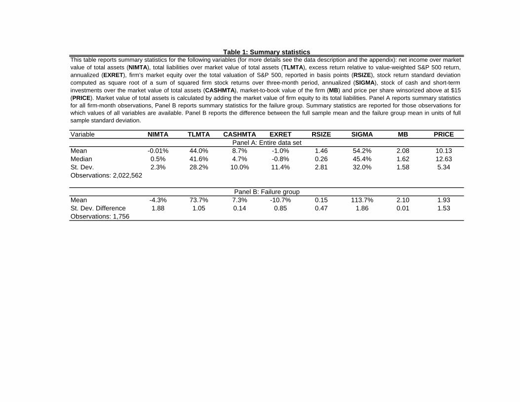
Table 1 reports summary statistics for these eight measures. Panel A reports sum-mary statistics for the full sample of �rm-months that we use to model failure pre-diction. Panel B reports statistics for the sample of �rms that fail over the followingmonth. The table also reports the di¤erence in means in units of standard deviation.

5

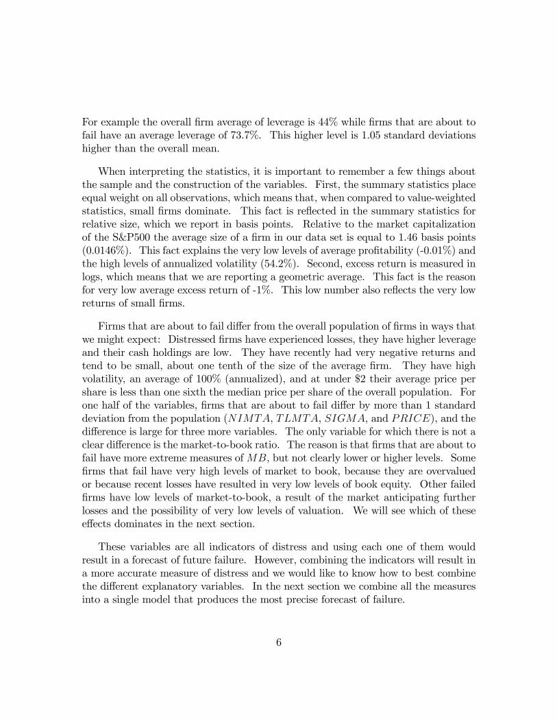
For example the overall �rm average of leverage is 44% while �rms that are about tofail have an average leverage of 73.7%. This higher level is 1.05 standard deviationshigher than the overall mean.

When interpreting the statistics, it is important to remember a few things aboutthe sample and the construction of the variables. First, the summary statistics placeequal weight on all observations, which means that, when compared to value-weightedstatistics, small �rms dominate. This fact is re�ected in the summary statistics forrelative size, which we report in basis points. Relative to the market capitalizationof the S&P500 the average size of a �rm in our data set is equal to 1.46 basis points(0.0146%). This fact explains the very low levels of average pro�tability (-0.01%) andthe high levels of annualized volatility (54.2%). Second, excess return is measured inlogs, which means that we are reporting a geometric average. This fact is the reasonfor very low average excess return of -1%. This low number also re�ects the very lowreturns of small �rms.

Firms that are about to fail di¤er from the overall population of �rms in ways thatwe might expect: Distressed �rms have experienced losses, they have higher leverageand their cash holdings are low. They have recently had very negative returns andtend to be small, about one tenth of the size of the average �rm. They have highvolatility, an average of 100% (annualized), and at under $2 their average price pershare is less than one sixth the median price per share of the overall population. Forone half of the variables, �rms that are about to fail di¤er by more than 1 standarddeviation from the population (NIMTA, TLMTA, SIGMA, and PRICE), and thedi¤erence is large for three more variables. The only variable for which there is not aclear di¤erence is the market-to-book ratio. The reason is that �rms that are about tofail have more extreme measures ofMB, but not clearly lower or higher levels. Some�rms that fail have very high levels of market to book, because they are overvaluedor because recent losses have resulted in very low levels of book equity. Other failed�rms have low levels of market-to-book, a result of the market anticipating furtherlosses and the possibility of very low levels of valuation. We will see which of thesee¤ects dominates in the next section.

These variables are all indicators of distress and using each one of them wouldresult in a forecast of future failure. However, combining the indicators will result ina more accurate measure of distress and we would like to know how to best combinethe di¤erent explanatory variables. In the next section we combine all the measuresinto a single model that produces the most precise forecast of failure.

6

3 A model predicting �nancial distress

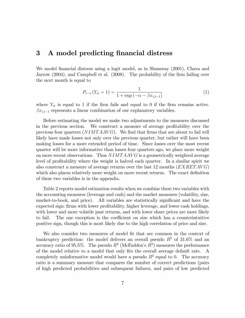
We model �nancial distress using a logit model, as in Shumway (2001), Chava andJarrow (2004), and Campbell et al. (2008). The probability of the �rm failing overthe next month is equal to

Pt�1 (Yit = 1) =1

1 + exp (��� �xi;t�1)(1)

where Yit is equal to 1 if the �rm fails and equal to 0 if the �rm remains active.�xi;t�1 represents a linear combination of our explanatory variables.

Before estimating the model we make two adjustments to the measures discussedin the previous section. We construct a measure of average pro�tability over theprevious four quarters (NIMTAAV G). We �nd that �rms that are about to fail willlikely have made losses not only over the previous quarter, but rather will have beenmaking losses for a more extended period of time. Since losses over the most recentquarter will be more informative than losses four quarters ago, we place more weighton more recent observations. ThusNIMTAAV G is a geometrically weighted averagelevel of pro�tability where the weight is halved each quarter. In a similar spirit wealso construct a measure of average returns over the last 12 months (EXRETAV G)which also places relatively more weight on more recent returns. The exact de�nitionof these two variables is in the appendix.

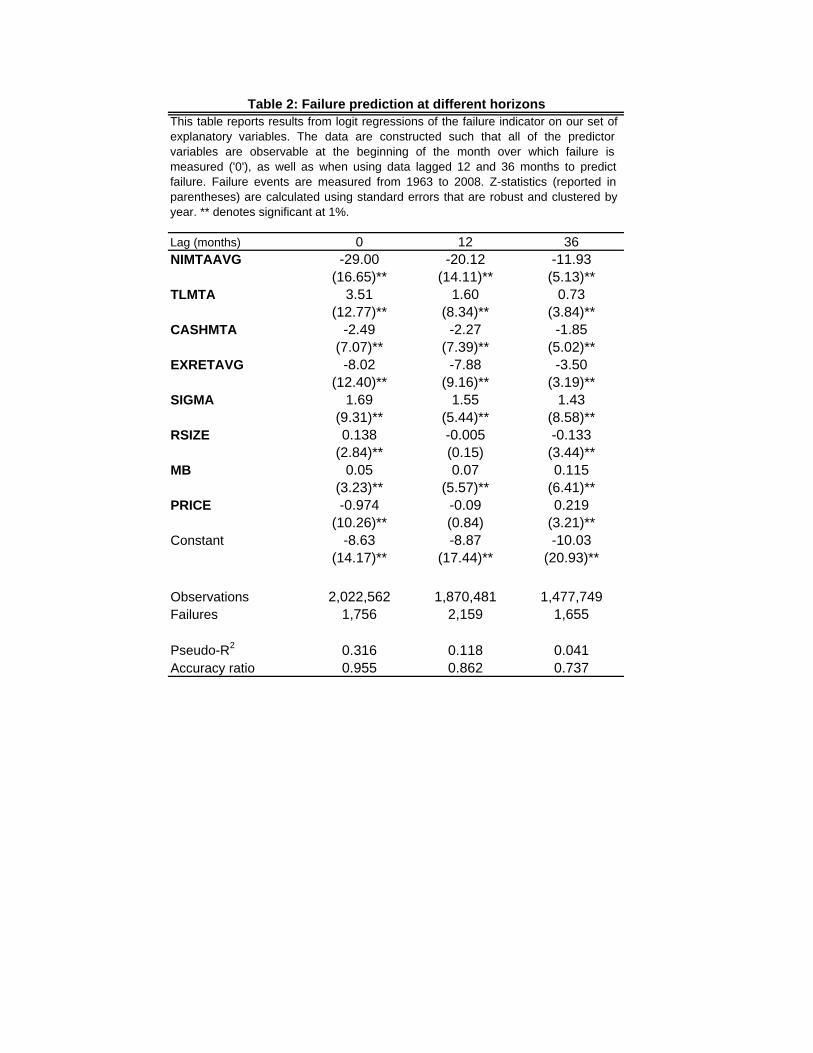
Table 2 reports model estimation results when we combine these two variables withthe accounting measures (leverage and cash) and the market measures (volatility, size,market-to-book, and price). All variables are statistically signi�cant and have theexpected sign: �rms with lower pro�tability, higher leverage, and lower cash holdings,with lower and more volatile past returns, and with lower share prices are more likelyto fail. The one exception is the coe¢ cient on size which has a counterintuitivepositive sign, though this is most likely due to the high correlation of price and size.

We also consider two measures of model �t that are common in the context ofbankruptcy prediction: the model delivers an overall pseudo R2 of 31.6% and anaccuracy ratio of 95.5%. The pseudo R2 (McFadden�s R2) measures the performanceof the model relative to a model that only �ts the overall average default rate. Acompletely uninformative model would have a pseudo R2 equal to 0. The accuracyratio is a summary measure that compares the number of correct predictions (pairsof high predicted probabilities and subsequent failures, and pairs of low predicted

7

probabilities and no subsequent failures) to the number of incorrect predictions. Anuninformative model would deliver an accuracy ratio of 50%.

Since investors will care not only about modeling �nancial distress over the nextmonth but will also be interested in the determinants of failure in the future, weconsider di¤erent prediction horizons. We estimate the probability of failure 12months in the future, given that the �rm has not failed over the next 12 months andwe do the same for 36 months. We report estimation results in the second and thirdcolumns of Table 2.

When predicting failure in 1 year and in 3 years, all the variables remain statisti-cally signi�cant and come in with the expected signs, with the only exception againbeing the coe¢ cients on price. At the 1-year horizon the coe¢ cient loses signi�-cance and at the 3-year horizon, price comes in with a positive sign. Meanwhile,size comes in with the expected sign �larger �rms are less likely to fail. This meansthat the variables have �ipped signs relative to the 1 month prediction horizon. Thise¤ect is again likely driven by their high level of correlation and the possibility ofunmodeled nonlinearities in the e¤ects of these two variables. We also �nd that atlonger horizons the more persistent characteristics of the �rm such as volatility andthe market-to-book ratio become relatively more important.

Not surprisingly, it is much more di¢ cult to forecast �nancial distress farther intothe future. Both measures of accuracy drop signi�cantly as the prediction horizonis lengthened. At 1 year the Pseudo R2 is equal to 11.8% and at 3 years it is 4.1%,while the accuracy ratio drops to 86.2% and 73.7% respectively. Nevertheless, evenat longer horizons, our model has a very high level of predictive ability.

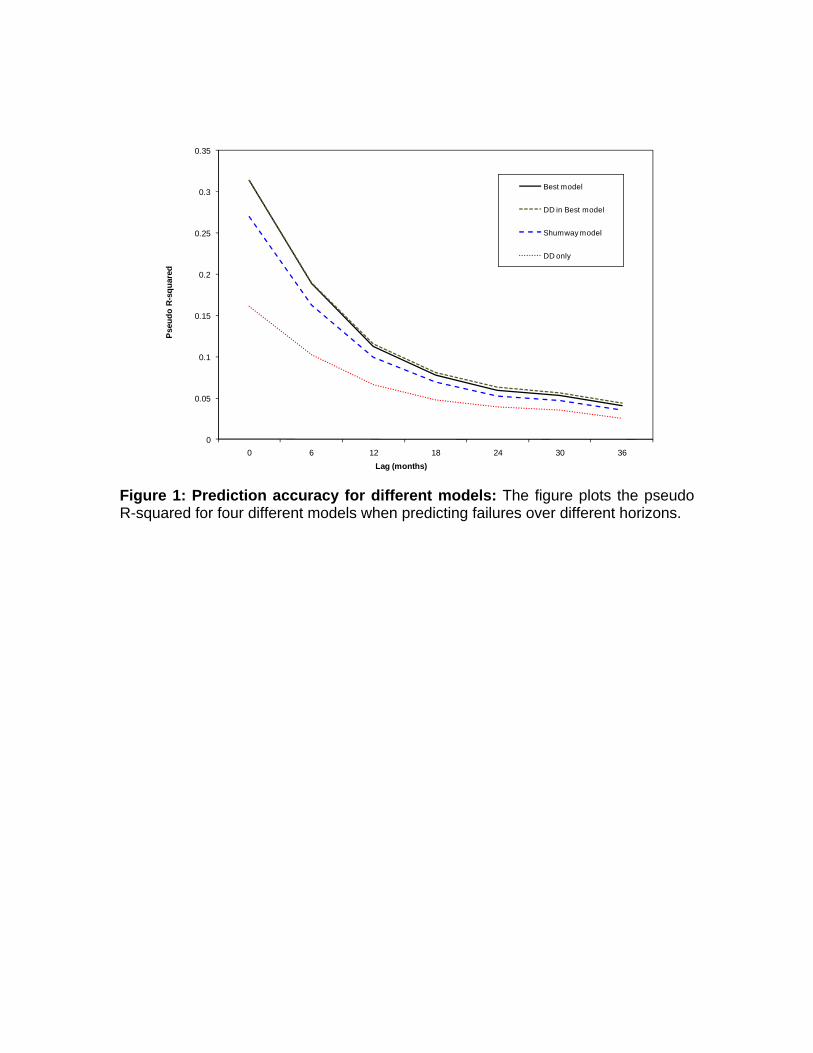
We next compare our model, which we will refer to as our �best model�to leadingalternatives. Our model takes as a starting point the model proposed by Shumway(2001) and used by Chava and Jarrow (2004), and �ve of our eight explanatoryvariables are closely related to variables used in these models. It is, therefore, naturalto consider our model�s performance relative to the Shumway (2001) model. We alsocompare our model�s performance to a common alternative, one used especially bypractitioners: distance-to-default. The model, popularized by Moody�s KMV, takesthe insights from option pricing used in the Merton (1974) model of risky debt andapplies them to the task of bankruptcy prediction. It assumes that a �rm entersbankruptcy if in one year�s time the market value of assets lies below the face valueof debt. Distance-to-default has been shown to be a predictor of future default (e.g.Vassalou and Xing (2004) and Hillegeist et al (2004)). We compare its performance

8

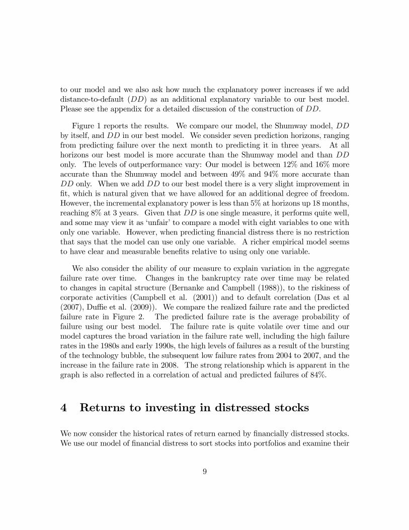
to our model and we also ask how much the explanatory power increases if we adddistance-to-default (DD) as an additional explanatory variable to our best model.Please see the appendix for a detailed discussion of the construction of DD.

Figure 1 reports the results. We compare our model, the Shumway model, DDby itself, and DD in our best model. We consider seven prediction horizons, rangingfrom predicting failure over the next month to predicting it in three years. At allhorizons our best model is more accurate than the Shumway model and than DDonly. The levels of outperformance vary: Our model is between 12% and 16% moreaccurate than the Shumway model and between 49% and 94% more accurate thanDD only. When we add DD to our best model there is a very slight improvement in�t, which is natural given that we have allowed for an additional degree of freedom.However, the incremental explanatory power is less than 5% at horizons up 18 months,reaching 8% at 3 years. Given that DD is one single measure, it performs quite well,and some may view it as �unfair�to compare a model with eight variables to one withonly one variable. However, when predicting �nancial distress there is no restrictionthat says that the model can use only one variable. A richer empirical model seemsto have clear and measurable bene�ts relative to using only one variable.

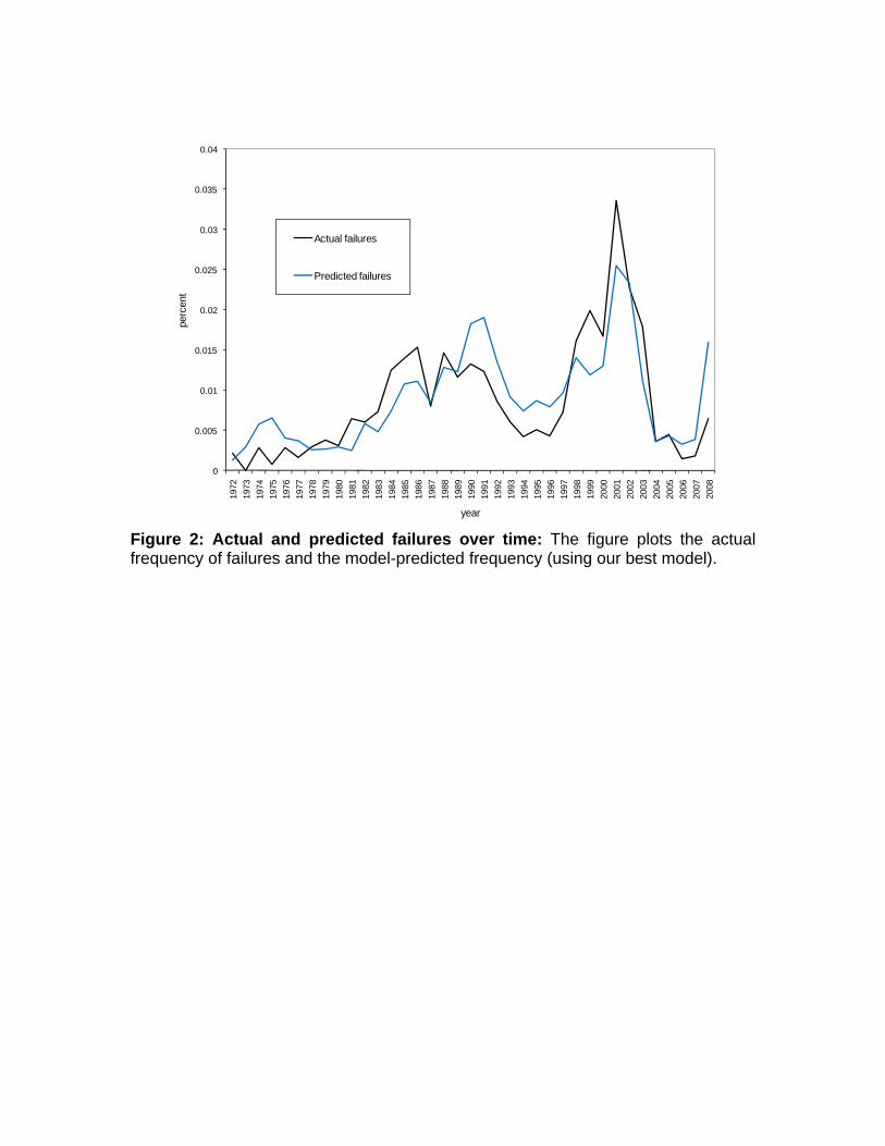
We also consider the ability of our measure to explain variation in the aggregatefailure rate over time. Changes in the bankruptcy rate over time may be relatedto changes in capital structure (Bernanke and Campbell (1988)), to the riskiness ofcorporate activities (Campbell et al. (2001)) and to default correlation (Das et al(2007), Du¢ e et al. (2009)). We compare the realized failure rate and the predictedfailure rate in Figure 2. The predicted failure rate is the average probability offailure using our best model. The failure rate is quite volatile over time and ourmodel captures the broad variation in the failure rate well, including the high failurerates in the 1980s and early 1990s, the high levels of failures as a result of the burstingof the technology bubble, the subsequent low failure rates from 2004 to 2007, and theincrease in the failure rate in 2008. The strong relationship which is apparent in thegraph is also re�ected in a correlation of actual and predicted failures of 84%.

4 Returns to investing in distressed stocks

We now consider the historical rates of return earned by �nancially distressed stocks.We use our model of �nancial distress to sort stocks into portfolios and examine their

9

returns from 1981 to 2008. The pronounced variation in the failure rate re�ected inFigure 2 suggests that variations in the failure rate are not idiosyncratic and cannotbe diversi�ed away. This means that investors should demand a premium for holdingthem.

Every January we sort �rms into 10 portfolios using the 12-month ahead proba-bility of failure from Table 3. In choosing the composition of the portfolios we payspecial attention to portfolios containing stocks with very low and very high failureprobabilities. The �rst portfolio contains those stocks with the lowest �ve percent ofthe failure probability distribution (0005), the second portfolio contains the next �vepercent of stocks, those with failure probabilities between the 5th and 10th percentileof the distribution (0510). We construct the next eight portfolios similarly so that wecover the entire spectrum of distress risk: 1020, 2040, 4060, 6080, 8090, 9095, 9599,and 9900, which invests in the �rms with the top 1% of the failure probabilities. Wealso consider a portfolio that goes long the safest 10% of stocks and short the mostdistressed 10% (LS1090).

To avoid look-ahead bias we re-estimate the model coe¢ cients every year. Forexample, we use data up to December 1990 to estimate the coe¢ cients on the eightvariables in our model, calculate failure probabilities, and then sort stocks into port-folios in January 1991. We hold stocks for one year and calculate value-weightedreturns. To reduce turnover, we do not rebalance portfolios during the year, butinstead use weights that drift with the performance of the stocks.

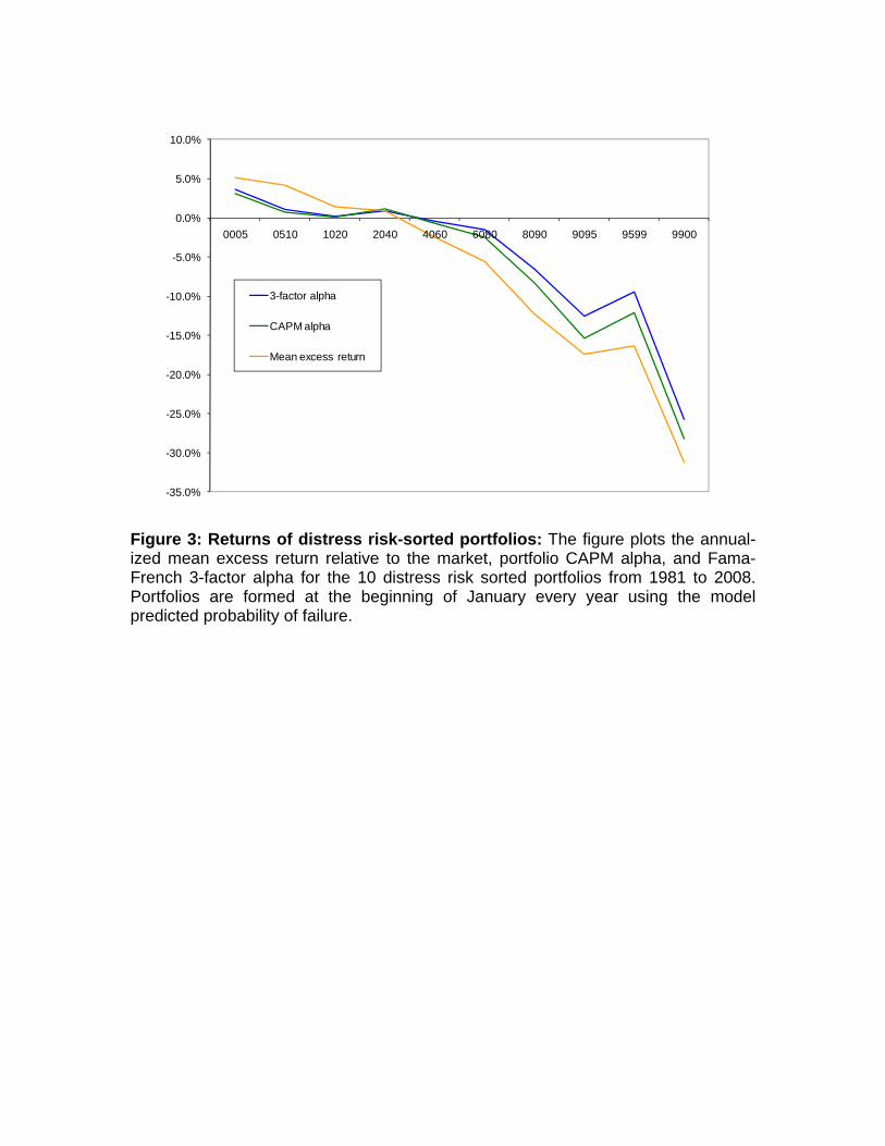
Table 3 reports average returns (Panel A) and characteristics (Panel B) for the 11portfolios. We �nd an almost monotonic relationship between distress and returns,though not in the direction one might expect: safe stocks have earned high returns,while distressed stocks have had very low returns. Average excess returns relative toS&P500 index returns are negative starting with portfolio 4060; they are statisticallysigni�cant at the 5% level for portfolio 8090, and signi�cant at the 1% level for thethree most distressed portfolios. The 1% most distressed stocks have underperformedthe S&P500 index by 26% (annualized monthly return). Table 3 Panel A also reportsCAPM alphas as well as alphas from the Fama and French (1993) three factor modeland the four factor model proposed by Carhart (1997). We use returns for the factorsfrom Ken French�s website to estimate these alphas. Figure 3 graphically summarizesthe pattern in returns across di¤erent levels of distress.

Panel B reports characteristics of the portfolios�constituent stocks. As expected,distressed stocks are more risky than safe stocks. The three most distressed stock

10

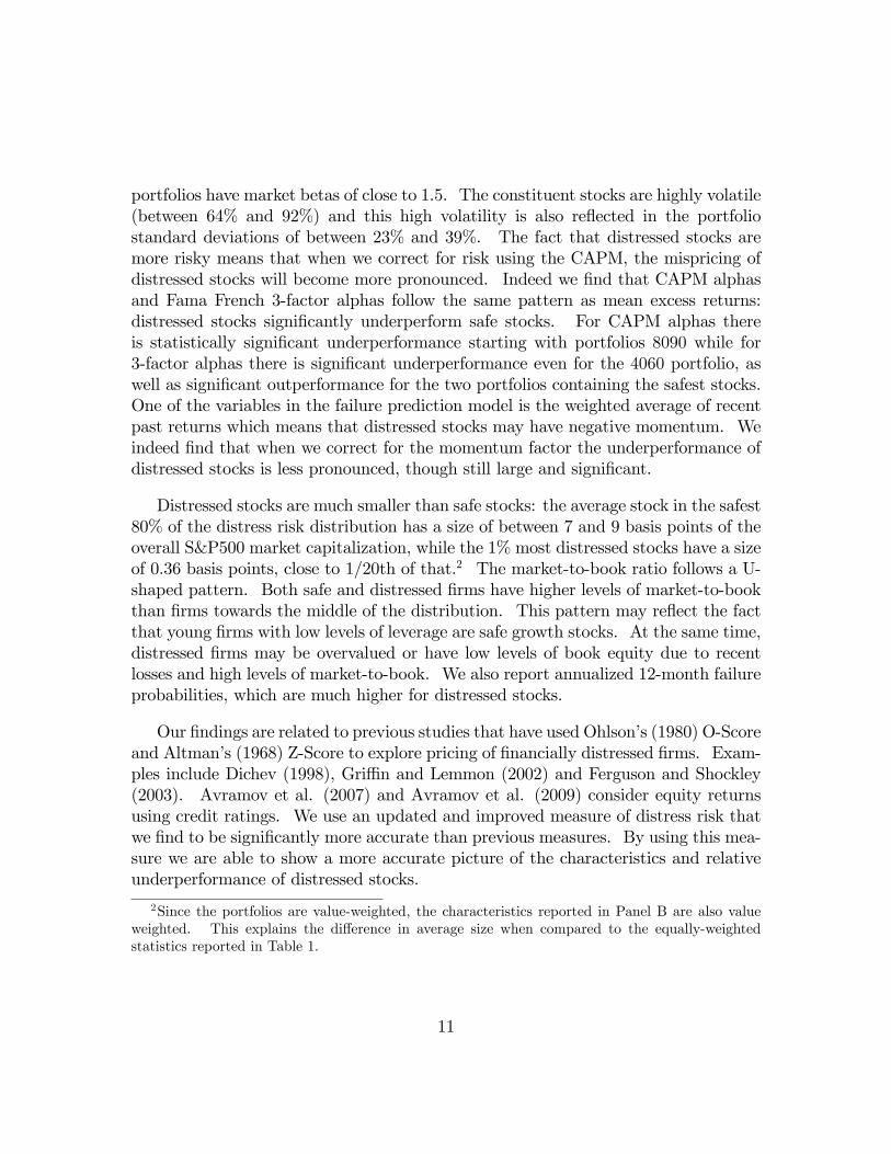
portfolios have market betas of close to 1.5. The constituent stocks are highly volatile(between 64% and 92%) and this high volatility is also re�ected in the portfoliostandard deviations of between 23% and 39%. The fact that distressed stocks aremore risky means that when we correct for risk using the CAPM, the mispricing ofdistressed stocks will become more pronounced. Indeed we �nd that CAPM alphasand Fama French 3-factor alphas follow the same pattern as mean excess returns:distressed stocks signi�cantly underperform safe stocks. For CAPM alphas thereis statistically signi�cant underperformance starting with portfolios 8090 while for3-factor alphas there is signi�cant underperformance even for the 4060 portfolio, aswell as signi�cant outperformance for the two portfolios containing the safest stocks.One of the variables in the failure prediction model is the weighted average of recentpast returns which means that distressed stocks may have negative momentum. Weindeed �nd that when we correct for the momentum factor the underperformance ofdistressed stocks is less pronounced, though still large and signi�cant.

Distressed stocks are much smaller than safe stocks: the average stock in the safest80% of the distress risk distribution has a size of between 7 and 9 basis points of theoverall S&P500 market capitalization, while the 1% most distressed stocks have a sizeof 0.36 basis points, close to 1/20th of that.2 The market-to-book ratio follows a U-shaped pattern. Both safe and distressed �rms have higher levels of market-to-bookthan �rms towards the middle of the distribution. This pattern may re�ect the factthat young �rms with low levels of leverage are safe growth stocks. At the same time,distressed �rms may be overvalued or have low levels of book equity due to recentlosses and high levels of market-to-book. We also report annualized 12-month failureprobabilities, which are much higher for distressed stocks.

Our �ndings are related to previous studies that have used Ohlson�s (1980) O-Scoreand Altman�s (1968) Z-Score to explore pricing of �nancially distressed �rms. Exam-ples include Dichev (1998), Gri¢ n and Lemmon (2002) and Ferguson and Shockley(2003). Avramov et al. (2007) and Avramov et al. (2009) consider equity returnsusing credit ratings. We use an updated and improved measure of distress risk thatwe �nd to be signi�cantly more accurate than previous measures. By using this mea-sure we are able to show a more accurate picture of the characteristics and relativeunderperformance of distressed stocks.

2Since the portfolios are value-weighted, the characteristics reported in Panel B are also valueweighted. This explains the di¤erence in average size when compared to the equally-weightedstatistics reported in Table 1.

11

4.1 Performance of distressed stocks across characteristicsand over time

The pronounced pattern of size and value across the distress-risk sorted portfoliossuggests that the underperformance of distressed stocks may be related to their char-acteristics. We therefore now consider the performance of distressed stocks acrossportfolios sorted on size and value. For both characteristics we sort �rst on size andvalue, then on distress. We use the NYSE breakpoints from Ken French�s websiteto do the sorting. We then calculate 3-factor alphas on portfolios long the safestquintile, short the most distressed quintile.

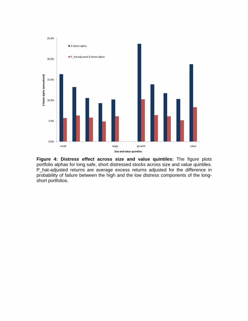
Figure 4 reports the results. We �nd a clear pattern across size-sorted portfolioswith annualized alphas of 16.3% for small �rms, compared to 10.2% for large �rms.Though the outperformance is larger for small �rms, this may be driven by a largerspread in distress risk between safe and risky small stocks. This is likely giventhat distressed �rms are much smaller. We correct for the higher spread in distressfor smaller stocks by calculating 3-factor alphas scaled by the di¤erence in failureprobability (�P̂ -adjusted 3-factor alpha�) and �nd that the di¤erence in performanceis driven entirely by the higher spread in distress risk for small �rms.

We also compare the relative performance of safe and distressed stocks acrossportfolios sorted on value. The underperformance of distressed stocks is more pro-nounced for extreme growth and value stocks. The 3-factor alphas for the highestand the lowest quintile of the book-to-market distribution are almost twice as largeas the alphas for the three middle groups. We again adjust for the dispersion infailure probability and �nd that the large performance gap for the extreme portfoliosis partly driven by the larger spread in the failure probability P̂ . The 3-factor alphaand the P̂ -adjusted 3-factor alpha are all statistically signi�cant (18 of 20 coe¢ cientsat the 1% level, and 2 coe¢ cients at the 5% level). We conclude that the under-performance of �nancially distressed stocks is present across the entire spectrum ofthe size and value distributions and is not concentrated only in a particular group of�rms.

One possibility for the underperformance of distressed stocks might be that in-vestors are unaware of some companies�level of �nancial distress or that it is di¢ cultfor investors to easily borrow stocks of distressed �rms that they can short sell. Inother words, it is possible that the underperformance of distressed stocks is concen-trated in �rms that have informational or arbitrage related frictions.

12

We consider this hypothesis by comparing performance across stocks with di¤er-ent levels of analyst coverage. If �rms have high analyst coverage it is likely thatinformation is more easily available and that news about �rms�prospects reachesmarket participants more quickly. Since there is a strong relationship between sizeand analyst coverage �large stocks tend to have higher analyst coverage than smallstocks �we correct for the e¤ect of size on analyst coverage by calculating residualanalyst coverage (following Hong, Lim, and Stein (2001)). This way we include bothlarge and small stocks that have lower analyst coverage than other stocks of com-parable size. We then sort �rst on the top and bottom third of the distribution ofresidual analyst coverage, then on distress.

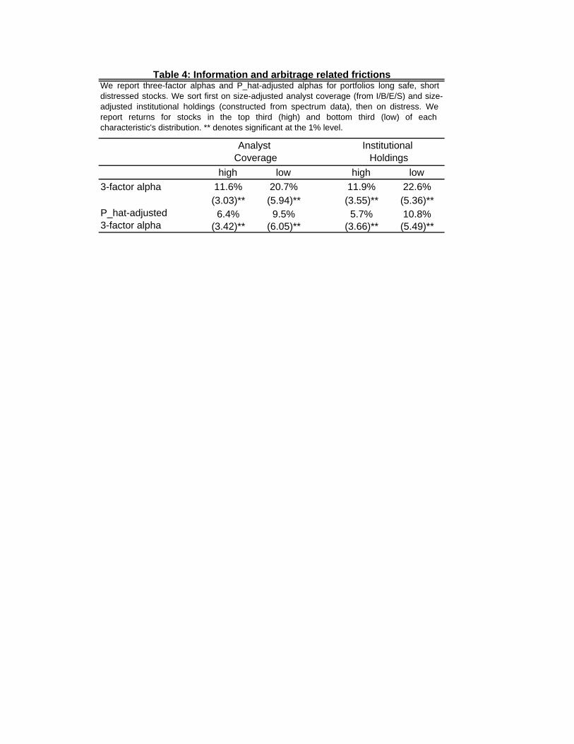
Table 4 reports the results. We �nd that the relative underperformance of dis-tressed stocks, measured by their 3-factor alphas, is about twice as large for �rmswith low analyst coverage. The di¤erence in P̂ -adjusted 3-factor alphas is smallerwhich means that the e¤ect is partly driven by a higher dispersion in distress forlower analyst coverage stocks.

We also consider whether or not there is a relationship between the level of in-stitutional holdings and the performance of distressed stocks. Higher institutionalholding may be viewed as a proxy for the relative availability of stocks that can beborrowed for short-selling purposes and that can be arbitraged by institutional in-vestors (see, for example, Nagel (2005)). Similar to analyst coverage, institutionalholdings also have a strong pattern across size so we calculate residual institutionalholdings before sorting stocks into the top and bottom third of the distribution. We�nd that the underperformance of distressed stocks is again about twice as large forlow institutional holding stocks. The relative magnitude is similar for P̂ -adjusted3-factor alphas.

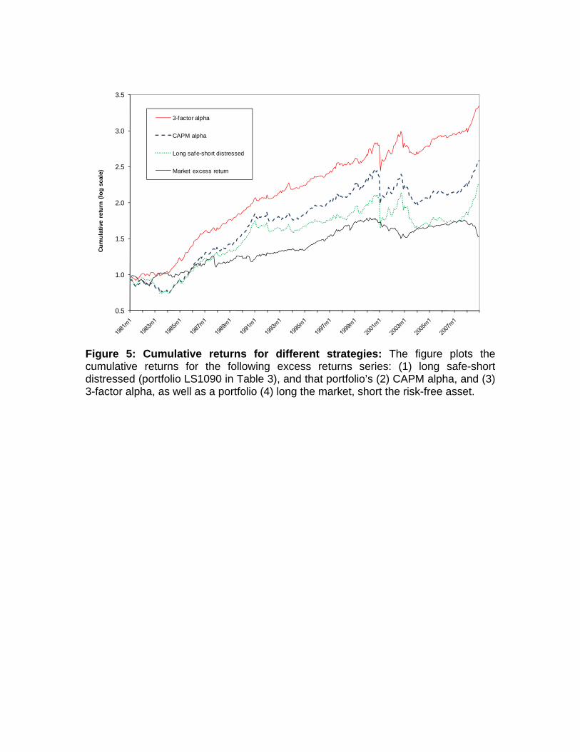
It is also possible that the underperformance of distressed stocks is very concen-trated. It may also have been reduced over time as investors have become moreaware of the pattern. We consider this hypothesis and next examine the relativeperformance of distressed stocks over time. Figure 5 reports the cumulative perfor-mance of the portfolio long the safest 10% of stocks and short the most distressed 10%(LS1090 in Table 3), from 1981 to 2008. The �gure plots cumulative excess returns,CAPM alphas and 3-factor alphas. For comparison we also report the cumulativeexcess return of the S&P500 relative to the risk-free rate. (We use monthly risk freereturns from Ken French�s data library.)

The graph illustrates the performance of the long-short portfolio relative to the

13

market portfolio. Over the entire period the long-short portfolio has outperformedthe market, which re�ects the signi�cant excess return we report in Table 3. Once weadjust for risk the outperformance of the long safe, short distressed strategy widens,again consistent with the results reported in Table 3. A long-short strategy withinitial size of $1 and invested in from January 1981 to December 2008 resulted in$3.41 (market return relative to the risk-free rate), $18.33 (long safe-short distressed),$38.60 (CAPM alpha) and $220.92 (3-factor alpha). The Sharpe ratios of the fourstrategies over the period are equal to 37% (market), 55% (long safe-short distressed),67% (CAPM alpha) and 97% (3-factor alpha).

Figure 5 also illustrates that there are risks associated with the long-short strategyand that returns have not been uniformly high. Excess returns and CAPM alphasare somewhat concentrated in the period from 1984 to 1991 as well as from 2003to 2008. Also, cumulative returns of the long-short strategy over the period from2000 to the second quarter of 2008 have been close to zero (though, not surprisingly,they were very high from September to December 2008). The performance for risk-adjusted returns (CAPM alpha and 3-factor alpha) is much more consistent overtime. In addition, especially since 2000, the long safe-short distressed portfolio hastended to have high returns during times of low market returns. Table 3 reportsthat the CAPM beta of the long-short portfolio is equal to -0.47 and this negativebeta is re�ected in the graph: The market downturns of 2001/2002 and 2008 are bothassociated with strong performance of the long-short portfolio, while the market rallyof 2003 is associated with low returns of the long-short strategy.

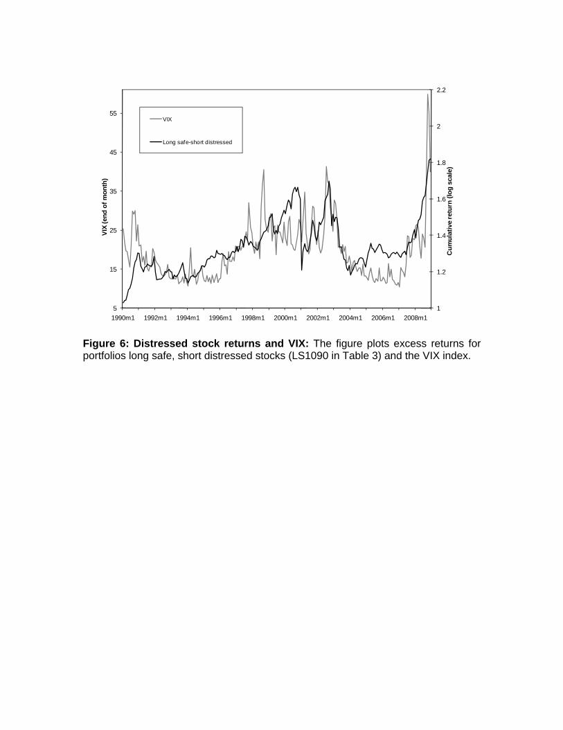
It is possible that investors do not perceive distressed stocks as risky and thereforedo not demand compensation for taking on risk. However, if instead distressedstocks are viewed by investors as risky and if they are viewed as marginal, then wemight expect distressed stocks to do particularly poorly at times of heightened marketuncertainty and at times during which investors are reluctant to hold risky assets.As a proxy for such times we use the VIX index, the implied volatility of the S&P500.During times of high market volatility, we might expect a ��ight to quality e¤ect,�which leads investors to bid up the prices of safe stocks relative to those that aredistressed. We would also expect such a pattern given the evidence of a positivecorrelation between credit spreads and the VIX index (see, for example, Berndt et al.(2005), and Schaefer and Strebulaev (2008)).

Figure 6 plots the cumulative return on the long safe-short distressed portfolio (thesame as in Figure 5) and the VIX index from 1990 to 2008 (the time during with the

14

VIX is available). The graph illustrates the pattern that we might expect: distressedstocks do relatively more poorly during times of heightened market volatility andrisk aversion. The graph also re�ects the correlation of long safe-short distressed andcontemporaneous changes in the VIX of 24% (monthly frequency) and 42% (quarterlyfrequency).

5 Conclusion

In this paper we consider the measurement and pricing of stocks in �nancial dis-tress. We �rst present a model of �nancial distress that predicts corporate failureusing accounting and market-based variables. The model�s predictions are intuitive:distressed �rms are those that have recently made losses, have high leverage, lowand volatile recent returns, have levels of market-to-book and low share prices. Ourbest model outperforms leading alternatives such as the model proposed by Shumway(2001) as well as distance-to-default, an approach popular in industry and one use byVassalou and Xing (2004) as well as Hillegeist et al. (2004).

In the second part of the paper we consider the performance of distressed stocksfrom 1981 to 2008. We �nd that distressed stocks have signi�cantly underperformedthe S&P500 and that they are risky � they have high levels of volatility and highmarket betas. This means that once we adjust for risk using the CAPM and FamaFrench 3-factor model, the apparent mispricing of distressed stocks worsens.

The strong underperformance of distressed stocks is a puzzle. We examine itfurther by considering three hypotheses: is the underperformance concentrated in�rms with particular characteristics, is it more pronounced for �rms with lower levelsof available information, or is it concentrated at particular points in time?

We �nd that the underperformance of distressed relative to safe stocks is presentacross all size and value quintiles, though it is more pronounced for portfolios thathave a larger spread in failure probability, a fact that explains the more extremeunderperformance of distressed stocks for small �rms. Furthermore, we �nd thatthe low performance of distressed stocks is concentrated in stocks with lower analystcoverage and lower institutional holdings. We interpret this fact as suggesting thatfor some distressed �rms it may be di¢ cult to easily gain information about their�nancial health and it may not be possible to short-sell severely distressed stocks.

15

The potential barriers to arbitrage may be one reason why there have continued tobe times of strong underperformance throughout our sample period.

What does all of this mean in practice? Our results suggest that investors shouldstay away from investing in distressed stocks. Furthermore, it should be quite possiblefor investors to collect information about �rms� health using the measures in ourmodel. Investing more heavily in safe stocks will reduce a diversi�ed portfolio�svolatility and its beta while increasing its returns. When possible, investors shouldalso short sell �rms in distress.

It seems unlikely that investors are not informed well enough to realize the op-portunities that they seem to be missing. We present a measure that is straightforward to construct and that investors could easily get access to. A more plausibleexplanation is that for some stocks short selling is constrained. This constraint maycause prices of distressed stocks to stay too high for too long. However, we �nd thatthe underperformance of distressed stocks is still present for large �rms, for �rms withhigher than average analyst coverage and with high levels of institutional holdings.For those stocks we might expect pro�ts to decline in the future.

In many areas of quantitative equity investing, pro�ts have declined over time dueto increased entry into the market and the resulting increase in competition (Khan-dani and Lo (2007)). The return to a strategy investing in safe stocks and shortingdistressed stocks does not seem to be an obvious exception to this pattern. Thereare clear risks associated with a long-short strategy, pro�ts have not been uniformlyhigh, and over the last decade a simple long short strategy has only marginally out-performed the market. However, a strategy long safe, short distressed stocks hasa very appealing quality in that returns seem to be concentrated in down markets.Furthermore, once adjusting for risk, the returns have been more stable and there hasbeen less evidence of a decline in pro�ts.

16

AppendixIn this appendix we discuss issues related to the construction of our data set and

restrictions for the inclusion in our estimation sample. All variables are constructedusing COMPUSTAT and CRSP data.

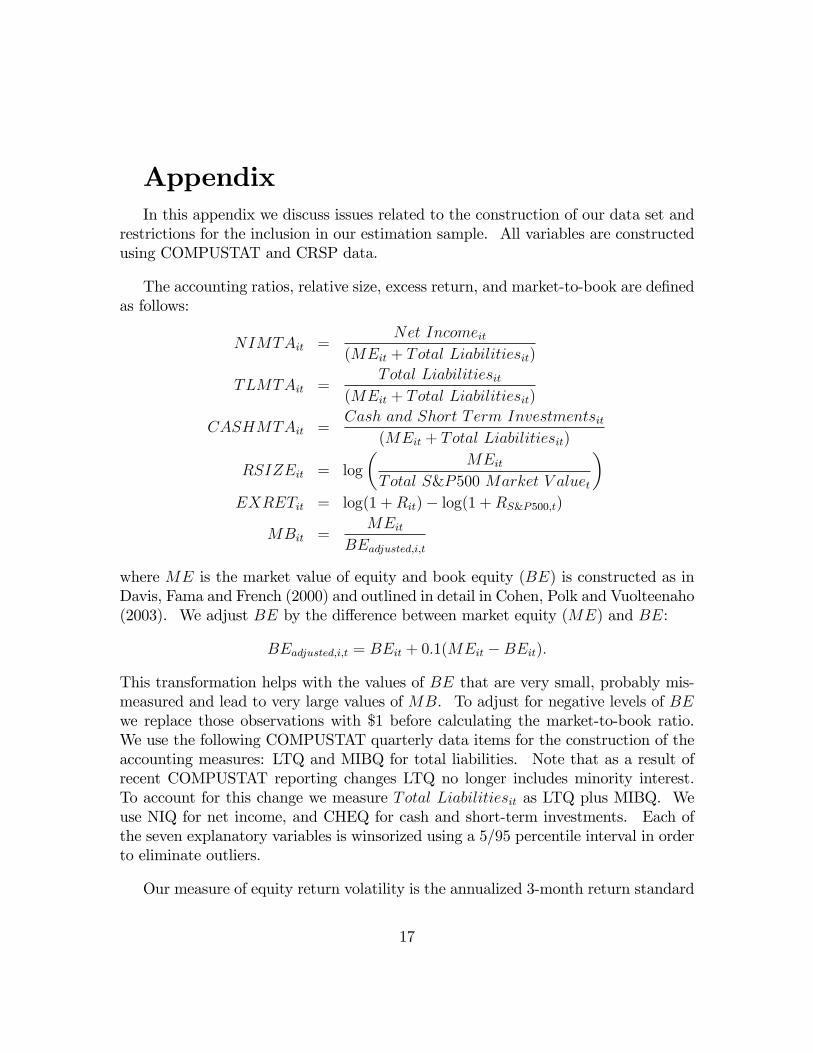
The accounting ratios, relative size, excess return, and market-to-book are de�nedas follows:

NIMTAit =Net Incomeit

(MEit + Total Liabilitiesit)

TLMTAit =Total Liabilitiesit

(MEit + Total Liabilitiesit)

CASHMTAit =Cash and Short Term Investmentsit

(MEit + Total Liabilitiesit)

RSIZEit = log

�MEit

Total S&P500 Market V aluet

�EXRETit = log(1 +Rit)� log(1 +RS&P500;t)

MBit =MEit

BEadjusted;i;t

where ME is the market value of equity and book equity (BE) is constructed as inDavis, Fama and French (2000) and outlined in detail in Cohen, Polk and Vuolteenaho(2003). We adjust BE by the di¤erence between market equity (ME) and BE:

BEadjusted;i;t = BEit + 0:1(MEit �BEit):

This transformation helps with the values of BE that are very small, probably mis-measured and lead to very large values of MB. To adjust for negative levels of BEwe replace those observations with $1 before calculating the market-to-book ratio.We use the following COMPUSTAT quarterly data items for the construction of theaccounting measures: LTQ and MIBQ for total liabilities. Note that as a result ofrecent COMPUSTAT reporting changes LTQ no longer includes minority interest.To account for this change we measure Total Liabilitiesit as LTQ plus MIBQ. Weuse NIQ for net income, and CHEQ for cash and short-term investments. Each ofthe seven explanatory variables is winsorized using a 5/95 percentile interval in orderto eliminate outliers.

Our measure of equity return volatility is the annualized 3-month return standard

17

deviation centered around zero:

SIGMAi;t�1;t�3 =

0@252 � 1

N � 1X

k2ft�1;t�2;t�3g

r2i;k

1A 12

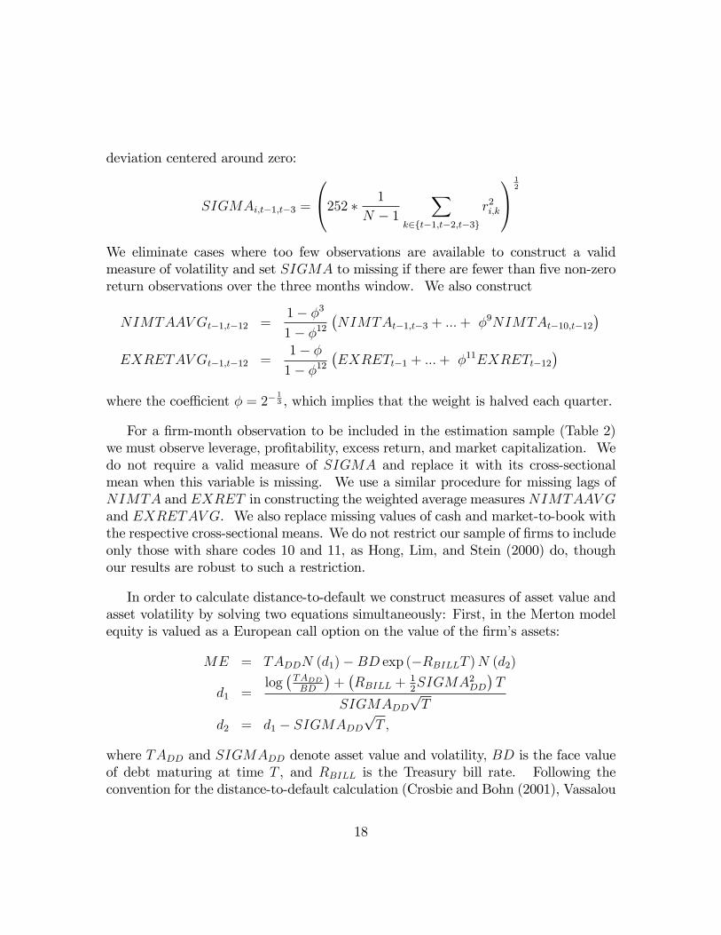
We eliminate cases where too few observations are available to construct a validmeasure of volatility and set SIGMA to missing if there are fewer than �ve non-zeroreturn observations over the three months window. We also construct

NIMTAAV Gt�1;t�12 =1� �3

1� �12�NIMTAt�1;t�3 + :::+ �9NIMTAt�10;t�12

�EXRETAV Gt�1;t�12 =

1� �1� �12

�EXRETt�1 + :::+ �11EXRETt�12

�where the coe¢ cient � = 2�

13 , which implies that the weight is halved each quarter.

For a �rm-month observation to be included in the estimation sample (Table 2)we must observe leverage, pro�tability, excess return, and market capitalization. Wedo not require a valid measure of SIGMA and replace it with its cross-sectionalmean when this variable is missing. We use a similar procedure for missing lags ofNIMTA and EXRET in constructing the weighted average measures NIMTAAV Gand EXRETAV G. We also replace missing values of cash and market-to-book withthe respective cross-sectional means. We do not restrict our sample of �rms to includeonly those with share codes 10 and 11, as Hong, Lim, and Stein (2000) do, thoughour results are robust to such a restriction.

In order to calculate distance-to-default we construct measures of asset value andasset volatility by solving two equations simultaneously: First, in the Merton modelequity is valued as a European call option on the value of the �rm�s assets:

ME = TADDN (d1)�BD exp (�RBILLT )N (d2)

d1 =log�TADDBD

�+�RBILL +

12SIGMA2DD

�T

SIGMADDpT

d2 = d1 � SIGMADDpT ;

where TADD and SIGMADD denote asset value and volatility, BD is the face valueof debt maturing at time T , and RBILL is the Treasury bill rate. Following theconvention for the distance-to-default calculation (Crosbie and Bohn (2001), Vassalou

18

and Xing (2004)), we assume T = 1, and use short term plus one half long term bookdebt to proxy for BD.

The second equation is a relation between equity volatility and asset volatility:

SIGMA = N (d1)TADDME

SIGMADD:

We solve the two equations numerically to �nd values for TADD and SIGMADDthat are consistent with the inputs. Before calculating asset value and volatility, weadjust BD so that BD=(ME + BD) is winsorized at the 0.5 and 99.5 percentiles ofthe cross-sectional distribution and winsorize SIGMA at the same percentline levels.We do this to reduce cases for which the numerical algorithm does not converge. Wethen compute distance to default as

DD =� log(BD=TADD) + 0:06 +RBILL � 1

2SIGMA2DD

SIGMADD:

The number 0.06 appears in the formula as an empirical proxy for the equity premium.We view using this measure as less noisy than using e.g. the average stock returnover the previous year, an approach employed in previous studies.

19

References

Altman, Edward I., 1968, Financial ratios, discriminant analysis and the predictionof corporate bankruptcy, Journal of Finance 23, 589�609.

Avramov, Doron, Tarun Chordia, Gergana Jostova, and Alexander Philipov, 2009,Credit ratings and the cross-section of stock returns, Journal of Financial Mar-kets 12, 469�499.

Avramov, Doron, Tarun Chordia, Gergana Jostova, and Alexander Philipov, 2007,Momentum and credit rating, Journal of Finance 62, 2503�2520.

Beaver, William H., 1966, Financial ratios as predictors of failure, Journal of Ac-counting Research 4, 71�111.

Beaver, William H., Maureen F. McNichols, and Jung-Wu Rhie, 2005, Have �nancialstatements become less informative? Evidence from the ability of �nancialratios to predict bankruptcy, Review of Accounting Studies.

Bernanke, Ben S. and John Y. Campbell, 1988, Is there a corporate debt crisis?,Brookings Papers on Economic Activity 1, 83�139.

Berndt, Antje, Rohan Douglas, Darrell Du¢ e, Mark Ferguson, and David Schranz,2005, Measuring default-risk premia from default swap rates and EDFs, workingpaper, Stanford University.

Bharath, Sreedhar and Tyler Shumway, 2004, Forecasting default with the Mertondistance to default model, Review of Financial Studies 21, 1339�1369.

Campbell John Y., Jens Hilscher, and Jan Szilagyi, 2008, In search of distress risk,Journal of Finance, 63, 2899�2939.

Campbell, John Y., Martin Lettau, Burton Malkiel, and Yexiao Xu, 2001, Have indi-vidual stocks become more volatile? An empirical exploration of idiosyncraticrisk, Journal of Finance 56, 1�43.

Carhart, Mark, 1997, On persistence in mutual fund performance, Journal of Fi-nance 52, 57�82.

Chan, K.C. and Nai-fu Chen, 1991, Structural and return characteristics of smalland large �rms, Journal of Finance 46, 1467�1484.

20

Chava, Sudheer and Robert A. Jarrow, 2004, Bankruptcy prediction with industrye¤ects, Review of Finance 8, 537�569.

Cohen, Randolph B., Christopher Polk and Tuomo Vuolteenaho, 2003, The valuespread, Journal of Finance 58, 609�641.

Crosbie, Peter J. and Je¤rey R. Bohn, 2001, Modeling Default Risk, KMV, LLC,San Francisco, CA.

Das, Sanjiv R., Darrell Du¢ e, Nikunj Kapadia, and Leandro Saita, 2007, Commonfailings: How corporate defaults are correlated, Journal of Finance 57, 93�117.

Davis, James L., Eugene F. Fama and Kenneth R. French, 2000, Characteristics,covariances, and average returns: 1929 to 1997, Journal of Finance 55, 389�406.

Dichev, Ilia, 1998, Is the risk of bankruptcy a systematic risk?, Journal of Finance53, 1141�1148.

Du¢ e, Darrell, Leandro Saita, and Ke Wang, 2007, Multi-period corporate defaultprediction with stochastic covariates, Journal of Financial Economics 83, 635�665.

Du¢ e, Darrell, Andreas Eckner, Guillaume Horel, and Leandro Saita, 2006, Frailtycorrelated default, Journal of Finance 66, 2089-2123.

Fama, Eugene F. and Kenneth R. French, 1993, Common risk factors in the returnson stocks and bonds, Journal of Financial Economics 33, 3�56.

Ferguson, Michael F. and Richard L. Shockley, 2003, Equilibrium �anomalies�, Jour-nal of Finance 58, 2549�2580.

Gilson, Stuart C., Kose John, and Larry Lang, 1990, Troubled debt restructurings:An empirical study of private reorganization of �rms in default, Journal ofFinancial Economics 27, 315�353.

Gilson, Stuart C., 1997, Transactions costs and capital structure choice: Evidencefrom �nancially distressed �rms, Journal of Finance 52, 161�196.

Gri¢ n, John M. and Michael L. Lemmon, 2002, Book-to-market equity, distress risk,and stock returns, Journal of Finance 57, 2317�2336.

21

Hillegeist, Stephen A., Elizabeth Keating, Donald P. Cram and Kyle G. Lunstedt,2004, Assessing the probability of bankruptcy, Review of Accounting Studies 9,5�34.

Hilscher, Jens, and Mungo Wilson, 2009, Credit ratings and credit risk, unpublishedpaper, Brandeis University and Oxford University.

Khandani, Amir E., and Andrew W. Lo, 2007, What happened to the Quants inAugust 2007? Journal of Investment Management 5, 29-78.

Hong, Harrison, Terence Lim, and Jeremy C. Stein, 2000, Bad news travels slowly:Size, analyst coverage, and the pro�tability of momentum strategies, Journalof Finance 55, 265�295.

Merton, Robert C., 1974, On the pricing of corporate debt: the risk structure ofinterest rates, Journal of Finance 29, 449�470.

Nagel, Stefan, 2005, Short sales, institutional investors and the cross-section of stockreturns, Journal of Financial Economics 78, 277�309.

Ohlson, James A., 1980, Financial ratios and the probabilistic prediction of bank-ruptcy, Journal of Accounting Research 18, 109�131.

Schaefer, Stephen M., and Ilya A. Strebulaev, 2008, Structural models of credit riskare useful: Evidence from hedge ratios on corporate bonds, Journal of FinancialEconomics 90, 1-19.

Shumway, Tyler, 2001, Forecasting bankruptcy more accurately: a simple hazardmodel, Journal of Business 74, 101�124.

Vassalou, Maria and Yuhang Xing, 2004, Default risk in equity returns, Journal ofFinance 59, 831�868.

22

Variable NIMTA TLMTA CASHMTA EXRET RSIZE SIGMA MB PRICE

Mean -0.01% 44.0% 8.7% -1.0% 1.46 54.2% 2.08 10.13Median 0.5% 41.6% 4.7% -0.8% 0.26 45.4% 1.62 12.63St. Dev. 2.3% 28.2% 10.0% 11.4% 2.81 32.0% 1.58 5.34Observations: 2,022,562

Mean -4.3% 73.7% 7.3% -10.7% 0.15 113.7% 2.10 1.93St. Dev. Difference 1.88 1.05 0.14 0.85 0.47 1.86 0.01 1.53Observations: 1,756

Panel A: Entire data set

Panel B: Failure group

Table 1: Summary statisticsThis table reports summary statistics for the following variables (for more details see the data description and the appendix): net income over marketvalue of total assets (NIMTA), total liabilities over market value of total assets (TLMTA), excess return relative to value-weighted S&P 500 return,annualized (EXRET), firm’s market equity over the total valuation of S&P 500, reported in basis points (RSIZE), stock return standard deviationcomputed as square root of a sum of squared firm stock returns over three-month period, annualized (SIGMA), stock of cash and short-terminvestments over the market value of total assets (CASHMTA), market-to-book value of the firm (MB) and price per share winsorized above at $15(PRICE). Market value of total assets is calculated by adding the market value of firm equity to its total liabilities. Panel A reports summary statisticsfor all firm-month observations, Panel B reports summary statistics for the failure group. Summary statistics are reported for those observations forwhich values of all variables are available. Panel B reports the difference between the full sample mean and the failure group mean in units of fullsample standard deviation.

Lag (months) 0 12 36NIMTAAVG -29.00 -20.12 -11.93

(16.65)** (14.11)** (5.13)**TLMTA 3.51 1.60 0.73

(12.77)** (8.34)** (3.84)**CASHMTA -2.49 -2.27 -1.85

(7.07)** (7.39)** (5.02)**EXRETAVG -8.02 -7.88 -3.50

(12.40)** (9.16)** (3.19)**SIGMA 1.69 1.55 1.43

(9.31)** (5.44)** (8.58)**RSIZE 0.138 -0.005 -0.133

(2.84)** (0.15) (3.44)**MB 0.05 0.07 0.115

(3.23)** (5.57)** (6.41)**PRICE -0.974 -0.09 0.219

(10.26)** (0.84) (3.21)**Constant -8.63 -8.87 -10.03

(14.17)** (17.44)** (20.93)**

Observations 2,022,562 1,870,481 1,477,749Failures 1,756 2,159 1,655

Pseudo-R2 0.316 0.118 0.041Accuracy ratio 0.955 0.862 0.737

Table 2: Failure prediction at different horizonsThis table reports results from logit regressions of the failure indicator on our set ofexplanatory variables. The data are constructed such that all of the predictorvariables are observable at the beginning of the month over which failure ismeasured ('0'), as well as when using data lagged 12 and 36 months to predictfailure. Failure events are measured from 1963 to 2008. Z-statistics (reported inparentheses) are calculated using standard errors that are robust and clustered byyear. ** denotes significant at 1%.

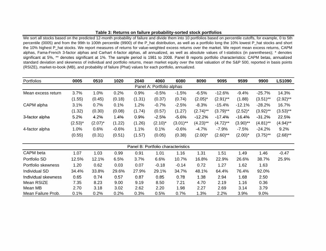
Table 3: Returns on failure probability-sorted stock portfoliosWe sort all stocks based on the predicted 12-month probability of failure and divide them into 10 portfolios based on percentile cutoffs, for example, 0 to 5thpercentile (0005) and from the 99th to 100th percentile (9900) of the P_hat distribution, as well as a portfolio long the 10% lowest P_hat stocks and shortthe 10% highest P_hat stocks. We report measures of returns for value-weighted excess returns over the market. We report mean excess returns, CAPMalphas, Fama-French 3-factor alphas and Carhart 4-factor alphas, all annualized, as well as absolute values of t-statistics (in parentheses); * denotessignificant at 5%, ** denotes significant at 1%. The sample period is 1981 to 2008. Panel B reports portfolio characteristics: CAPM betas, annualized

Portfolios 0005 0510 1020 2040 4060 6080 8090 9095 9599 9900 LS1090Panel A: Portfolio alphas

significant at 5%, denotes significant at 1%. The sample period is 1981 to 2008. Panel B reports portfolio characteristics: CAPM betas, annualizedstandard deviation and skewness of individual and portfolio returns, mean market equity over the total valuation of the S&P 500, reported in basis points(RSIZE), market-to-book (MB), and probability of failure (Phat) values for each portfolio, annualized.

Mean excess return 3.7% 1.0% 0.2% 0.9% -0.5% -1.5% -6.5% -12.6% -9.4% -25.7% 14.3%(1.55) (0.45) (0.18) (1.31) (0.37) (0.74) (2.05)* (2.91)** (1.88) (3.51)** (2.92)**

CAPM alpha 3.1% 0.7% 0.1% 1.2% -0.7% -2.5% -8.3% -15.4% -12.1% -28.2% 16.7%(1.32) (0.30) (0.08) (1.74) (0.57) (1.27) (2.74)** (3.79)** (2.52)* (3.92)** (3.53)**

3-factor alpha 5 2% 4 2% 1 4% 0 9% -2 5% -5 6% -12 2% -17 4% -16 4% -31 2% 22 5%

Panel A: Portfolio alphas

3-factor alpha 5.2% 4.2% 1.4% 0.9% -2.5% -5.6% -12.2% -17.4% -16.4% -31.2% 22.5%(2.53)* (2.07)* (1.22) (1.26) (2.10)* (3.01)** (4.23)** (4.72)** (3.90)** (4.81)** (4.94)**

4-factor alpha 1.0% 0.6% -0.6% 1.1% 0.1% -0.6% -4.7% -7.9% -7.5% -24.2% 9.2%(0.55) (0.31) (0.51) (1.57) (0.05) (0.38) (2.00)* (2.60)** (2.00)* (3.75)** (2.68)**

Panel B: Portfolio characteristicsCAPM beta 1.07 1.03 0.99 0.91 1.01 1.16 1.31 1.51 1.49 1.46 -0.47Portfolio SD 12.5% 12.1% 6.5% 3.7% 6.6% 10.7% 16.8% 22.9% 26.6% 38.7% 25.9%Portfolio skewness 1.20 0.62 0.03 0.07 -0.18 -0.14 0.72 1.27 1.62 1.63Individual SD 34.4% 33.8% 29.6% 27.9% 29.1% 34.7% 48.1% 64.4% 76.4% 92.0%Individual skewness 0 65 0 74 0 57 0 87 0 85 0 78 1 38 2 94 1 68 2 50

Panel B: Portfolio characteristics

Individual skewness 0.65 0.74 0.57 0.87 0.85 0.78 1.38 2.94 1.68 2.50Mean RSIZE 7.35 8.23 9.00 9.19 8.50 7.21 4.70 2.19 1.16 0.36Mean MB 2.70 3.18 3.02 2.62 2.20 1.98 2.27 2.69 3.14 3.79Mean Failure Prob. 0.1% 0.2% 0.2% 0.3% 0.5% 0.7% 1.3% 2.2% 3.9% 9.0%

high low high low3-factor alpha 11.6% 20.7% 11.9% 22.6%

(3.03)** (5.94)** (3.55)** (5.36)**6.4% 9.5% 5.7% 10.8%

(3.42)** (6.05)** (3.66)** (5.49)**

Table 4: Information and arbitrage related frictionsWe report three-factor alphas and P_hat-adjusted alphas for portfolios long safe, shortdistressed stocks. We sort first on size-adjusted analyst coverage (from I/B/E/S) and size-adjusted institutional holdings (constructed from spectrum data), then on distress. Wereport returns for stocks in the top third (high) and bottom third (low) of eachcharacteristic's distribution. ** denotes significant at the 1% level.

Analyst Coverage

Institutional Holdings

P_hat-adjusted 3-factor alpha

0

0.05

0.1

0.15

0.2

0.25

0.3

0.35

0 6 12 18 24 30 36

Pse

udo

R-s

quar

ed

Lag (months)

Best model

DD in Best model

Shumway model

DD only

Figure 1: Prediction accuracy for different models: The figure plots the pseudo R-squared for four different models when predicting failures over different horizons.

0

0.005

0.01

0.015

0.02

0.025

0.03

0.035

0.04

1972

1973

1974

1975

1976

1977

1978

1979

1980

1981

1982

1983

1984

1985

1986

1987

1988

1989

1990

1991

1992

1993

1994

1995

1996

1997

1998

1999

2000

2001

2002

2003

2004

2005

2006

2007

2008

perc

ent

year

Actual failures

Predicted failures

Figure 2: Actual and predicted failures over time: The figure plots the actual frequency of failures and the model-predicted frequency (using our best model).

-35.0%

-30.0%

-25.0%

-20.0%

-15.0%

-10.0%

-5.0%

0.0%

5.0%

10.0%

0005 0510 1020 2040 4060 6080 8090 9095 9599 9900

3-factor alpha

CAPM alpha

Mean excess return

Figure 3: Returns of distress risk-sorted portfolios: The figure plots the annual-ized mean excess return relative to the market, portfolio CAPM alpha, and Fama-French 3-factor alpha for the 10 distress risk sorted portfolios from 1981 to 2008. Portfolios are formed at the beginning of January every year using the model predicted probability of failure.

0.0%

5.0%

10.0%

15.0%

20.0%

25.0%

small large growth value

3‐factor alpha (annualized)

Size and value quintiles

3‐factor alpha

P_hat adjusted 3‐factor alpha 

Figure 4: Distress effect across size and value quintiles: The figure plots portfolio alphas for long safe, short distressed stocks across size and value quintiles. P_hat-adjusted returns are average excess returns adjusted for the difference in probability of failure between the high and the low distress components of the long-short portfolios.

0.5

1.0

1.5

2.0

2.5

3.0

3.5C

umul

ativ

e re

turn

(lo

g sc

ale)

3-factor alpha

CAPM alpha

Long safe-short distressed

Market excess return

Figure 5: Cumulative returns for different strategies: The figure plots the cumulative returns for the following excess returns series: (1) long safe-short distressed (portfolio LS1090 in Table 3), and that portfolio’s (2) CAPM alpha, and (3) 3-factor alpha, as well as a portfolio (4) long the market, short the risk-free asset.

1

1.2

1.4

1.6

1.8

2

2.2

5

15

25

35

45

55

1990m1 1992m1 1994m1 1996m1 1998m1 2000m1 2002m1 2004m1 2006m1 2008m1

Cum

ulat

ive

retu

rn (l

og s

cale

)

VIX

(end

of m

onth

)

VIX

Long safe-short distressed

Figure 6: Distressed stock returns and VIX: The figure plots excess returns for portfolios long safe, short distressed stocks (LS1090 in Table 3) and the VIX index.