Embed Size (px)
Citation preview

Computational Statistics and Data Analysis 56 (2012) 4081–4096
Contents lists available at SciVerse ScienceDirect
Computational Statistics and Data Analysis
journal homepage: www.elsevier.com/locate/csda
Predicting extreme value at risk: Nonparametric quantile regressionwith refinements from extreme value theoryJulia Schaumburg ∗
Humboldt-Universität zu Berlin, School of Business and Economics, Institute of Statistics and Econometrics, Chair of Econometrics, Spandauer Str. 1, 10178Berlin, Germany
a r t i c l e i n f o
Article history:Received 11 July 2011Received in revised form 22 March 2012Accepted 22 March 2012Available online 1 April 2012
Keywords:Value at riskNonparametric quantile regressionRisk managementExtreme value statistical applicationsMonotonization
a b s t r a c t
A framework is introduced allowing us to apply nonparametric quantile regression to Valueat Risk (VaR) prediction at any probability level of interest. A monotonized double kernellocal linear estimator is used to estimate moderate (1%) conditional quantiles of indexreturn distributions. For extreme (0.1%) quantiles, nonparametric quantile regression iscombined with extreme value theory. The abilities of the proposed estimators to capturemarket risk are investigated in a VaR prediction study with empirical and simulated data.Possibly due to its flexibility, the out-of-sample forecasting performance of the newmodelturns out to be superior to competing models.
© 2012 Elsevier B.V. All rights reserved.
1. Introduction
In bank regulation, the effectiveness of capital requirements in preventing funding shortfalls rests upon the estimationaccuracy of market risk measures, the most widely used of which is Value at Risk (VaR). According to the Market RiskAmendment to the Basel II Capital Accord of 2004, issued by the Bank for International Settlements, VaR is to be calculateddaily, using a ‘99th percentile, one-tailed confidence interval’.
Not only against the background of the financial turbulences during the crisis of 2007–2009, there is a practical needfor VaR models that are rich enough to capture the dynamics of quickly changing market environments, while beingparsimonious at the same time in order to avoid overfitting. In this context, kernel-based quantile regression is a naturalchoice. Being fully nonparametric, the approach does not require any structural assumptions, neither on the form of the VaRfunction nor on the shape of the loss distribution. Furthermore, as the primary interest is to predict quantiles accurately,not to estimate structural parameters, we do not lose interpretability by employing nonparametric estimation methods.
Until now, however, nonparametric quantile regression has not been widely used in risk management practice. Onepossible reason is that precisely because no structure is imposed on the regression function, the speed of convergenceis slower than in parametric regression settings, and generally more observations are needed for accurate estimation.Therefore, when considering nonparametric quantile regression for VaR prediction, one has to address the problem of datasparseness at the tails of the loss distribution, which getsmore severewhen considering quantiles corresponding to extremeprobabilities.
This paper proposes a framework allowing us to operationalize nonparametric quantile regression as a VaR estimationtool for both moderate and extreme probabilities. We include only past returns as regressors, which is sufficient, as amaximum of information can be exploited and any kinds of nonlinearities are captured within the modeling approach.
∗ Tel.: +49 0 30 2093 5603; fax: +49 0 30 2093 5712.E-mail address: [email protected].
0167-9473/$ – see front matter© 2012 Elsevier B.V. All rights reserved.doi:10.1016/j.csda.2012.03.016

4082 J. Schaumburg / Computational Statistics and Data Analysis 56 (2012) 4081–4096
In addition, the model is simple, overfitting is avoided and problems arising from limited observations are minimized. Adouble kernel-type estimator is used to smooth distortions. Additionally, monotonization by rearrangement is applied atthe boundary of the estimated function. Finally, in order to predict VaR corresponding to extreme probability levels (such as0.1%), the peaks over threshold method is incorporated and applied to the standardized nonparametric quantile residuals,resulting in an estimator that combines nonparametric quantile regression and extreme value theory (EVT).
Several studies have compared the forecast performances of different VaR models, see, among others, Kuester et al.(2006), Manganelli and Engle (2001) and Nieto and Ruiz (2008). They take a broad variety of models into account, butnonparametric quantile regression as a tool for VaR estimation is rarely included. There are three exceptionswe are aware of:Cai and Wang (2008) suggest estimating VaR and Expected Shortfall using a new nonparametric VaR estimator, combiningthe Weighted Nadaraya Watson (WNW) estimator of Cai (2002) and the Double Kernel Local Linear (DKLL) estimator ofYu and Jones (1998). In the empirical application, however, only 5% quantile curves are estimated and no forecasts arecomputed. Chen and Tang (2005) investigate nonparametric VaR estimation, when no regressors are present. Taylor (2008)proposes to combine double kernel quantile regression with exponential smoothing of the dependent variable in the timedomain. 1% and 99% VaRs are predicted from the model along with some benchmarks, but extreme quantiles are notconsidered. Although the Basel Committee on Banking Supervision asks banks to report VaR for a 10-day holding period, wefocus on one-day-ahead forecasts, which is in line with the literature.
In contrast to the studies already available in the literature, we present a method that allows us to nonparametricallyestimate VaR corresponding to any probability that might be of practical interest. We estimate, predict and backtest 1%and 0.1% VaRs for four sets of index returns and a simulated time series. Our focus is on gains to loosening assumptions incomparison to existing VaR models. Therefore, in the empirical application, we choose to benchmark our model against themost flexible parametric VaRmodels, the Conditional Autoregressive Value at Risk (CAViaR)models of Engle andManganelli(2004). They allow us to set up different linear and nonlinear specifications, including the lagged VaR estimate as a regressor,and they do not rely on distributional assumptions.
We find that although the CAViaR models obtain almost perfect in-sample fits in the case of 1% VaR, the Double KernelLocal Linear (DKLL) estimator of Yu and Jones (1998) often outperforms them in terms of out-of-sample backtesting results,especially when the estimation period is short relative to the forecasting period. Results are promising for 0.1% VaR as well.The superiority of the EVT-refined DKLL estimator over the plain DKLL estimator is shown in a small simulation study. Itturns out that, especially when the estimation window is small relative to the forecasting period, the extreme value theory-refined nonparametric model predicts extreme VaRs very accurately.
Section 2 outlines the basic setup of conditional quantile models, before describing CAViaR models. The DKLL estimatorused in the following is presented in Section 3. Furthermore, the incorporation of extreme value theory into the model isexplained. The investigated data sets and the backtesting method are summarized in Section 4. The empirical results on 1%and 0.1% VaR estimation are stated in Section 5. In Section 6, the performance of the EVT-refined nonparametric model isfurther assessed via a small simulation study. Section 7 concludes.
2. Quantile regression approaches to VaR estimation
2.1. Conditional quantiles
Let Ytnt=1 be a strictly stationary time series of portfolio returns and let Xt be a d-dimensional vector of regressors. The
pth conditional quantile of Yt , denoted by qp(x), is defined as
qp(x) = inf y ∈ R : F(y|x) ≥ p ≡ F−1(p|x), (2.1)
or, equivalently, as the argument that solves
minqp(x)
Ep − I(Yt < q(Xt))
Yt − q(Xt)
|Xt = x
, (2.2)
where I(A) denotes the indicator function on some set A. Both formulations are widely used in the literature. In the seminalpaper by Koenker and Bassett (1978) a sample equivalent of (2.2) where q(Xt) = X′
tβ, also including the special caseXt = 1,is established. β is a d-dimensional vector of unknown parameters. The linear quantile model is extended to conditionallyheteroskedastic processes in Koenker and Zhao (1996). In Engle and Manganelli (2004) conditional autoregressive quantilefunctions are estimated using (2.2) with q(Xt) possibly being nonlinear in parameters, see Section 2.2 for some examples.In a number of papers, localized kernel versions of (2.2) are estimated, leading to a nonparametric fit: Yu and Jones (1997)compare the goodness of fit of local constant and local linear models. On the other hand, Cai (2002), Yu and Jones (1998)and Cai andWang (2008) propose nonparametric methods to estimate the distribution function in (2.1), which, in a secondstep, is inverted. Section 3.1 contains more details on these approaches. Wu et al. (2007) model (2.1) without regressors,and Chernozhukov and Umantsev (2001) operationalize a linear version of (2.1).
Following the convention of expressing VaR as a positive number, it is defined as
VaRtp(·) = −qtp(·),

J. Schaumburg / Computational Statistics and Data Analysis 56 (2012) 4081–4096 4083
where qtp is the quantile of the return distribution corresponding to probability p, at time t . VaRtp denotes a generic VaR
measure which may depend on x and/or a vector of parameters β. To simplify notation, index t is suppressed in contextswhere it does not cause confusion.
2.2. Conditional Autoregressive VaR (CAViaR) models
The class of Conditional Autoregressive Value at Risk (CAViaR) models, first introduced by Engle and Manganelli (2004),is used to benchmark the forecast performance of the nonparametric VaR estimators considered here. Several comparisonstudies have done so, for example Kuester et al. (2006) or Taylor (2008). CAViaRmodels are dynamic VaRmodels describingthe quantile of a random variable at time t , e.g. the return on a financial portfolio, as possibly nonlinear function of its ownlags and, in addition, of a vector of observable variables, Xt :
VaRtp(β) = β0 +
r1i=1
βiVaRt−ip (β) +
r2j=1
βjf (Xt−j),
where d = r1 + r2 + 1 is the dimension of β, the parameter vector that may be estimated by solving
minβ
1n
nt=1
p − I
Yt < −VaRt
p(β)
(Yt + VaRtp(β)). (2.3)
A straightforward choice for Xt is lagged returns. Following the original article, the specifications used here include the firstlagged value of VaRp(·) and the first lagged value of Yt , therefore Xt = Yt−1.
Well-known stylized facts on asset returns are, firstly, that they exhibit volatility clustering. It carries over to VaR: if highvariation is observed in returns of the recent past, it is likely to continue, and risk is therefore high aswell. Secondly, quantiles(or volatility) might react differently according to the sign of past returns. This possibility is captured by the AsymmetricSlope specification
VaRtp(β) = β1 + β2VaRt−1
p (β) + β3(Yt−1)+
+ β4(Yt−1)−, (2.4)
where (x)+ = max(x, 0) and (x)− = −min(x, 0), but not by the Indirect GARCH(1, 1) specification
VaRtp(β) =
β1 + β2(VaRt−1
p )2(β) + β3Y 2t−1. (2.5)
On the other hand, the Asymmetric Slope CAViaR imposes a piecewise linear structure on VaR, although the true functionalformmight be nonlinear. As pointed out in Kuester et al. (2006), financial returnsmay also have an autoregressive (AR)mean,which is neglected by the CAViaR specifications, which artificially set the mean return equal to zero. For these reasons wecombine the features of the above, by allowing for nonlinearity and asymmetric effects of past returns, and additionallyincorporate an AR mean, by introducing an alternative specification, called Indirect Autoregressive Threshold GARCH(AR-TGARCH(1, 1)) CAViaR:
VaRtp(β) = β1Yt−1 +
β2 + β3(VaRt−1
p )2(β) + β4Y 2t−1 + β5(Yt−1)
2I(Yt−1 < 0) 1
2 . (2.6)
Including the AR term introduces the possibility for a nonzero autoregressive mean, asymmetry is present if β5 = 0 and thesquare root allows for a nonlinear functional form.
For estimating the parameters of the CAViaR models, an algorithm similar to the one proposed in the original paper isapplied, see Engle and Manganelli (2004). A grid search is conducted by generating a large number of random vectors, thedimensions of which correspond to the number of model parameters. The five vectors which lead to the lowest values ofthe objective function (2.3) are selected and fed into a simplex optimization algorithm. The final parameter vector is chosento be the one minimizing (2.3). Our new AR-TGARCH specification fits into this procedure.
3. Nonparametric quantile regression with refinements from extreme value theory
3.1. Double Kernel Local Linear VaR regression
In general, estimating nonparametric models requires large amounts of data. Since VaR corresponds to a quantile at thetail of the return distribution, suitable nonparametric quantile estimators should be able to deal with areas where data aresparse. Therefore, from the variety of nonparametric quantile estimators, the Double Kernel Local Linear (DKLL) estimator ofYu and Jones (1998) is chosen for the VaR application, because it localizes the data in both the x- and y-direction, which leadsto smoother estimates. Formore details, regularity assumptions and asymptotic properties, see the original article by Yu andJones (1998). TheWeightedDouble Kernel Local Linear estimator of Cai andWang (2008), aNadarayaWatson type estimator,forms an alternative to the DKLL estimator. In a small simulation study, which is not reported here, the DKLL estimator per-formed slightly better at design points at the boundary of the support of the data. Therefore, we chose it for our application.

4084 J. Schaumburg / Computational Statistics and Data Analysis 56 (2012) 4081–4096
For notational convenience, observations (Xt , Yt)nt=1 are assumed to be drawn from underlying bivariate distribution
F(x, y) with density f (x, y). The extension to the multivariate case is straightforward, but requires a more tedious notation.The estimator is defined as the inverse of a conditional distribution function as in (2.1). Throughout this section, quantilesof return distributions are discussed, so that VaR corresponds to the negative quantile.
A generic nonparametric method of estimating a conditional distribution F(y|x) is
F(y|x) =
nt=1
wt(x)I(Yt ≤ y), (3.1)
where I(·) is again an indicator function and the weights wt(x) are positive and sum up to one. Choosing equal weightsw = 1/n yields the empirical distribution function. Using instead a kernel function with bandwidth parameter h, in thefollowing sometimes abbreviated by Kh(·) =
1hK(·/h), which is often chosen to be a symmetric probability density function,
results in the Nadaraya Watson estimator of a conditional distribution
FNW (y|x) =
nt=1
Kh(x − Xt)n
t=1Kh(x − Xt)
wt (x)
I(Yt ≤ y), (3.2)
see for example Li and Racine (2007). It attaches a smooth set ofweights to the data, and is known to bemonotone increasingand bounded between zero and one. However, it suffers from boundary distortion, as shown by Fan and Gijbels (1996). Theyadvocate the use of local polynomial estimators, the simplest of which is the local linear estimator.
One way to reduce distortions that arise due to a limited number of observations is to smooth not only the observationsof the regressor variable Xt , but also the observations of the dependent variable Yt . This requires the introduction of a secondsymmetric kernelWh2(·). Its kernel distribution, which is defined by y
−∞
Wh2(Yt − u)du = Ω
y − Yt
h2
, (3.3)
with h2 being the bandwidth parameter, can be viewed as a smooth, differentiable version of the indicator function.As a next step, the conditional distribution value of y is approximated by a linear Taylor expansion around x. The estimate
F(y|x) = β0 is obtained from
(β0, β1) = arg minβ0,β1
nt=1
Ω
y − Yt
h2
− β0 − β1(Xt − x)
2
Kh1 (x − Xt) , (3.4)
where h1 > h2. Solving for β0 yields the explicit expression for the conditional distribution function estimator,
F(y|x) =
nt=1
Kh1 (x − Xt) [S2 − (x − Xt)S1]n
t=1Kh1 (x − Xt) [S2 − (x − Xt)S1]
wt (x)
Ω
y − Yt
h2
, (3.5)
where
Sl =
ni=1
Kx − Xt
h1
(x − Xi)
l, l = 1, 2.
(3.5) is a version of (3.1) where the kernel distribution function Ω(·) in (3.3) replaces the indicator. The DKLL quantileestimator qp(x), the sample analogue to (2.1), is then defined by
qp(x) = infy ∈ ℜ : F(y|x) ≥ p
≡ F−1(p|x). (3.6)
with F from (3.5). In finite samples, F(y|x)might not always bemonotonically increasing. In such cases, however, the inverseis not defined. Yu and Jones (1998) suggest the following implementation scheme: for q1/2(x), any value satisfying (3.6) ischosen; for p > 1/2, the largest, and for p < 1/2, the smallest solutions to (3.6) are taken as quantile estimates.
In this paper, a stronger procedure is applied, to avoid deleting estimated values. Chernozhukov et al. (2009) show thatany nonmonotone estimate of a monotone function can be improved in terms of common metrics, such as the Lp-norm, bysimple rearranging. In an earlier work, Dette et al. (2006) propose a similar method of smoothed rearrangements. For thecase of amonotone increasing (decreasing) function, the point estimates are sorted in ascending (descending) order. Makinguse of these theoretical results, nonmonotone distribution estimates are rearranged before inverting. In the present contextof monotonizing the estimated distribution function, a further effect is that quantile crossing is circumvented. Estimatedvalues greater than one are discarded.

J. Schaumburg / Computational Statistics and Data Analysis 56 (2012) 4081–4096 4085
3.2. Refining nonparametric quantile regression with extreme value theory
For extreme quantiles, usually very few data points are available, so that fully nonparametric regression does not yieldreliable estimates. Extreme value theory (EVT) is an alternative to model extreme quantiles. In the following, a method ofincorporating extreme value theory into CAViaR models, which was introduced by Manganelli and Engle (2001), is adaptedto obtain 0.1% VaR estimates from a nonparametric model.
The strategy is to first calculate the standardized quantile residuals,
ϵtp2
qtp2=
Yt − qtp2qtp2
=Yt
qtp2− 1. (3.7)
p denotes the (very low) probability of interest, and p2 corresponds to a moderately low probability for which the quantilecanbe estimatednonparametrically, for example p2 = 0.01or p2 = 0.05.McNeil and Frey (2000) employ a similar techniqueto estimate 1% VaR from a GARCH residual series. An EVT-augmented nonparametric kernel distribution estimator is alsoconsidered by MacDonald et al. (2011), who show consistency of their method via a Bayesian inference.
Reformulating the definition of the pth quantile of portfolio returns in terms of the p2th quantile yields
P[Yt < qtp] = PYt < qtp2 − qtp2 + qtp
= P
Yt
qtp2− 1 >
qtpqtp2
− 1
= p.
The inequality sign is switched assuming that qtp2 is a negative number. Let
zp ≡qtpqtp2
− 1
denote the (1 − p)th quantile of the standardized residuals. It is then estimated by the peaks over threshold (POT) method,though it can be estimated by other methods, such as the Hill estimator, as well. A number of applications employ the POTmethod to forecast extreme quantiles; for a selection of applications and an investigation of its finite sample properties seeEl-Arouia and Diebolt (2002). An estimate for the pth return quantile can be expressed by means of zp and qtp2 :
qtpqtp2
− 1 = zp ⇔ qtp = qtp2(zp + 1). (3.8)
Again, VaRtp = −qtp. In the remainder of this section, the underlying extreme value arguments, which are used to obtain zp
in (3.8), are discussed very briefly, following Embrechts et al. (1997).Large observations which exceed a high threshold can be approximated reasonably well by the Generalized Pareto
Distribution (GPD) with distribution function
Gξ,β(x) =
−(1 + ξx/β)1/ξ for ξ = 01 − ex/β for ξ = 0,
(3.9)
with shape parameter ξ and scale parameter β > 0. The support is x ≥ 0 when ξ ≥ 0 and 0 ≤ x ≤ −β
ξif ξ < 0. The
parameters can be consistently estimated if the threshold exceedances are independent, regardless of the true underlyingdistribution, see Smith (1987). In general, given a high threshold u and a random variable Y , the probability of Y exceedingu at most by x is given by
Fu(x) = P[Y − u ≤ x|Y > u] =F(x + u) − F(u)
1 − F(u). (3.10)
Balkema and de Haan (1974) and Pickands (1975) show that for a large class of distribution functions F it is possible to finda positive function β(u) such that
limu→y0
sup0≤x<y0−u
Fu(x) − Gξ,β(u)(x) = 0, (3.11)
with y0 corresponding to the right endpoint of F . Rearranging (3.10) and using Fu(·) ≈ Gξ,β(·), it holds that
1 − F(u + x) ≈ [1 − F(u)][1 − Gξ,β(x)].
Then, 1 − Gξ,β(x) can be obtained by estimating the GPD parameters by maximum likelihood. Let Nu denote the number ofexceedances over threshold u. A common way of estimating S(u) := 1 − F(u) is to use the empirical distribution functionNun . Substituting the estimates,
S(u + x) =Nu
n
1 + ξ
x
β
−1ξ
. (3.12)

4086 J. Schaumburg / Computational Statistics and Data Analysis 56 (2012) 4081–4096
The quantile can be estimated by inverting (3.12), employing a change of variables y = u + x and fixing the distributionvalue at the probability of interest: F(y) = p. Therefore, the quantile estimator qp is obtained from
1 − p =Nu
n
1 + ξ
y − u
β
−1ξ
⇔qp = u +
(1 − p)
nNu
−ξ
− 1
·β
ξ. (3.13)
In general, extreme value methods require the underlying data to be i.i.d. Although computing standardized residuals asin (3.7) should remove most of the dynamics, one cannot eliminate the possibility of remaining autocorrelation. However,under some conditions on the dependence structure (see e.g. Drees, 2003, for details), the relationship between the limitingdistributions of the maxima of a dependent but strictly stationary sequence, (Yt)t∈N say, and a white noise sequence (Yt)t∈Nwith the same distribution function F may be described by the so-called extremal index θ ∈ (0, 1]. If the distribution ofnormalized threshold exceedances in the sequence (Yt) converges to an extreme value distribution G(x), as in (3.11), thenit can be shown that the equally normalized exceedances of (Yt)t∈N converge to Gθ (x), see Embrechts et al. (1997). Thus, thesame limiting extreme value distribution may be used, while changing only the normalization parameters.
Intuitively, if our sequence of standardized residuals possesses an extremal indexwhich is<1, then its extremal behavioris asymptotically the same as that of a shorter white noise sequence with the same distribution. However, it might still beinteresting to find out about the extent of deviation from white noise for a given data set. The extremal index may beestimated by the so-called Runs Method where θ is computed as the conditional probability that a threshold exceedance isfollowed by a run of r non-exceedances. The idea is that periods in between clusters of exceedances are longer than periodsbetween independent exceedances (for details see Embrechts et al., 1997, Chapter 8). The higher the clustering tendency,the fewer runs will be present. The estimator is
θ =
n−rt=1
I(At)
nt=1
I(Yt > u), (3.14)
where I(·) is again the indicator function and
At = Yt > u, Yt+1 ≤ u, . . . , Yt+r ≤ u . (3.15)
Drees (2003) shows that a wide variety of financial time series, including ARMA and ARCH processes, may be estimated bythe POT maximum likelihood estimator which we use here. He finds that the only difference to i.i.d. data is an increasedvariance of the quantile estimator, but this drawback does not affect our results, as our goal is forecasting accuracy, whichis checked via backtesting.
4. Data and backtesting method
We analyze four data sets of daily index returns, DAX, FTSE 100 (FTSE), EuroSTOXX 50 (EuroSTOXX) and S&P 500 (S&P).The longest available time series of each are used to compute in-sample fits. The common end date of the in-sample periodis 28/02/2003. We predict VaR for the subsequent 1000 days, until the end of 2006 (29/12/2006). As a second step, we takethe same forecast period, but additionally include 300 days to check whether model performances worsen when the datacontains the beginning of the financial crisis. The 1300-day forecast period ends on 22/02/2008. Table 1 summarizes somefeatures of the data.
The reason for using a rather long estimation period relative to the forecast horizon, is that our aim is to assess andcompare the quality of the nonparametric model in capturing market risk, using as much information as possible. We areaware that in real life risk management, available time series are typically much shorter. Therefore, in Section 5.2.2, weadditionally estimate our models using only the last 1000 data points, from 30/04/1999 to 28/02/2003 and forecast 1% VaRsfor the subsequent 200 and 1000 days. Realizations of quantiles cannot be observed. Therefore, backtesting of the modelsis carried out using the dynamic quantile (DQ) out-of-sample test developed in Engle and Manganelli (2004) to test andcompare the performance of VaR models. From the variety of alternatives, we choose this particular test, because it is thestandard test to compare CAViaR and other models. Define the binary variable
Hitt ≡ I(Yt < −VaRtp) − p.
If the chosen model is correct,
E[Hitt |Ωt ] = 0, (4.1)
where Ωt is any information known up to time t . Thus, VaR is estimated correctly, if independently for each day of theforecasting period, the probability of exceeding it equals p. Note that this also implies that Hitt is uncorrelated with its own
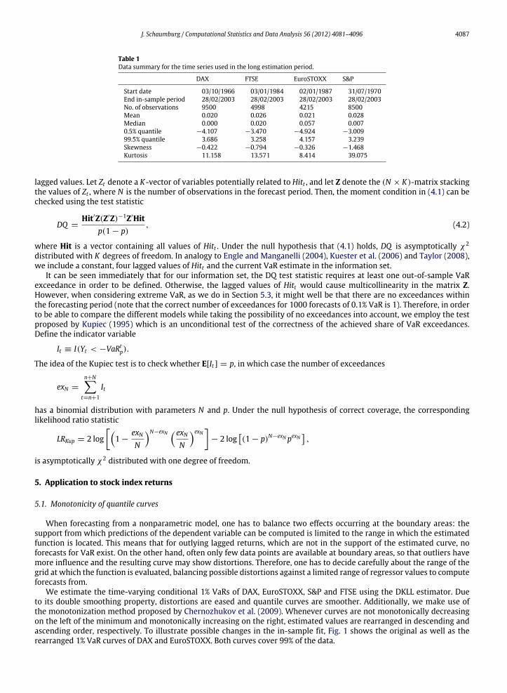
J. Schaumburg / Computational Statistics and Data Analysis 56 (2012) 4081–4096 4087
Table 1Data summary for the time series used in the long estimation period.
DAX FTSE EuroSTOXX S&P
Start date 03/10/1966 03/01/1984 02/01/1987 31/07/1970End in-sample period 28/02/2003 28/02/2003 28/02/2003 28/02/2003No. of observations 9500 4998 4215 8500Mean 0.020 0.026 0.021 0.028Median 0.000 0.020 0.057 0.0070.5% quantile −4.107 −3.470 −4.924 −3.00999.5% quantile 3.686 3.258 4.157 3.239Skewness −0.422 −0.794 −0.326 −1.468Kurtosis 11.158 13.571 8.414 39.075
lagged values. Let Zt denote a K -vector of variables potentially related to Hitt , and let Z denote the (N × K)-matrix stackingthe values of Zt , where N is the number of observations in the forecast period. Then, the moment condition in (4.1) can bechecked using the test statistic
DQ =Hit′Z(Z′Z)−1Z′Hit
p(1 − p), (4.2)
where Hit is a vector containing all values of Hitt . Under the null hypothesis that (4.1) holds, DQ is asymptotically χ2
distributed with K degrees of freedom. In analogy to Engle and Manganelli (2004), Kuester et al. (2006) and Taylor (2008),we include a constant, four lagged values of Hitt and the current VaR estimate in the information set.
It can be seen immediately that for our information set, the DQ test statistic requires at least one out-of-sample VaRexceedance in order to be defined. Otherwise, the lagged values of Hitt would cause multicollinearity in the matrix Z.However, when considering extreme VaR, as we do in Section 5.3, it might well be that there are no exceedances withinthe forecasting period (note that the correct number of exceedances for 1000 forecasts of 0.1% VaR is 1). Therefore, in orderto be able to compare the different models while taking the possibility of no exceedances into account, we employ the testproposed by Kupiec (1995) which is an unconditional test of the correctness of the achieved share of VaR exceedances.Define the indicator variable
It ≡ I(Yt < −VaRtp).
The idea of the Kupiec test is to check whether E[It ] = p, in which case the number of exceedances
exN =
n+Nt=n+1
It
has a binomial distribution with parameters N and p. Under the null hypothesis of correct coverage, the correspondinglikelihood ratio statistic
LRKup = 2 log
1 −exNN
N−exN exNN
exN
− 2 log(1 − p)N−exN pexN
,
is asymptotically χ2 distributed with one degree of freedom.
5. Application to stock index returns
5.1. Monotonicity of quantile curves
When forecasting from a nonparametric model, one has to balance two effects occurring at the boundary areas: thesupport from which predictions of the dependent variable can be computed is limited to the range in which the estimatedfunction is located. This means that for outlying lagged returns, which are not in the support of the estimated curve, noforecasts for VaR exist. On the other hand, often only few data points are available at boundary areas, so that outliers havemore influence and the resulting curve may show distortions. Therefore, one has to decide carefully about the range of thegrid at which the function is evaluated, balancing possible distortions against a limited range of regressor values to computeforecasts from.
We estimate the time-varying conditional 1% VaRs of DAX, EuroSTOXX, S&P and FTSE using the DKLL estimator. Dueto its double smoothing property, distortions are eased and quantile curves are smoother. Additionally, we make use ofthe monotonization method proposed by Chernozhukov et al. (2009). Whenever curves are not monotonically decreasingon the left of the minimum and monotonically increasing on the right, estimated values are rearranged in descending andascending order, respectively. To illustrate possible changes in the in-sample fit, Fig. 1 shows the original as well as therearranged 1% VaR curves of DAX and EuroSTOXX. Both curves cover 99% of the data.

4088 J. Schaumburg / Computational Statistics and Data Analysis 56 (2012) 4081–4096
Fig. 1. Original and rearranged DKLL estimates of 1% conditional DAX VaR curve (upper panel) EuroSTOXX VaR curve (lower panel).
Table 2 compares backtesting results on original and rearranged DKLL fits, on a forecast horizon of 1000 days. In-sampleand out-of-sample coverages are aimed to be as close as possible to the underlying probability, in this case 1%. The P-valueof the DQ test described in Section 4 expresses the highest significance level at which the variables in the information setare jointly significant. Therefore, a larger P-value indicates that the null hypothesis of independent VaR exceedances is morelikely not to be rejected, suggesting that a model is more adequate.
The theoretical results from Chernozhukov et al. (2009), that rearranging weakly improves estimation, are confirmedby our empirical results: Whenever values in the columns are different, they are superior for the rearranged estimates. In-sample and out-of-sample coverages are closer to 1% in case of the FTSE return series. Furthermore, the DQ test P-valuesubstantially increases, indicating that the null hypothesis of the DQ test is ‘further away’ from rejection than in the case ofthe original DKLL model. Whenever we mention results for the DKLL estimator in the following, it refers to the rearrangedversion.
5.2. Comparing 1% VaR predictions
5.2.1. Long estimation periodTable 3 lists backtest results of the CAViaR models and the rearranged DKLL estimates which are obtained from the large
data set described in Table 1. Generally, the in-sample exceedance shares achieved by all three CAViaR specifications are very

J. Schaumburg / Computational Statistics and Data Analysis 56 (2012) 4081–4096 4089
Table 2DQ test results for original and rearranged DKLL models as well as in-sample and out-ofsample share of VaR exceedances (in percent). The forecast period is 1000 observations.
DKLL orig. DKLL rearr. DKLL orig. DKLL rearr.
DAX FTSE
In-sample (%) 0.78 0.78 0.94 0.95Out-of-sample (%) 1.00 1.00 0.40 0.50DQ P-value 0.182 0.182 0.614 0.830
EuroSTOXX S&P
In-sample (%) 0.81 0.81 0.97 0.97Out-of-sample (%) 0.50 0.50 0.30 0.30DQ P-value 0.859 0.859 0.544 0.544
Table 3Backtesting results for 1% VaR models. In-sample and out-of-sample exceedanceprobabilities in %. Considered forecast horizons are 1000 and 1300 observations.
Asymm. slope GARCH AR-TGARCH DKLL
DAX
In-sample 1.01 1.01 1.04 0.78Out-of-sample (1000) 1.50 1.50 1.50 1.00Out-of-sample (1300) 1.54 1.54 1.61 1.07DQ P-value (1000) 0.054* 0.011** 0.054* 0.182DQ P-value (1300) 0.043** 0.009*** 0.039** 0.040**
FTSE
In-sample 1.02 1.00 1.00 0.94Out-of-sample (1000) 0.60 0.60 0.60 0.50Out-of-sample (1300) 1.08 1.16 1.08 1.00DQ P-value (1000) 0.005*** 0.007*** 0.007*** 0.830DQ P-value (1300) 0.040** 0.104 0.059* 0.011**
EuroSTOXX
In-sample 1.04 0.99 0.99 0.81Out-of-sample (1000) 0.70 0.80 0.80 0.50Out-of-sample (1300) 0.76 0.92 0.92 0.62DQ P-value (1000) 0.970 0.058* 0.057* 0.859DQ P-value (1300) 0.980 0.015** 0.015** 0.031**
S&P
In-sample 1.01 1.00 0.97 0.97Out-of-sample (1000) 0.30 0.30 0.30 0.30Out-of-sample (1300) 0.92 1.00 0.69 1.15DQ P-value (1000) 0.547 0.285 0.547 0.544DQ P-value (1300) 0.042** 0.000*** 0.079* 0.008***
* Model which is rejected by the DQ test for rejection at the 10% significance level.** Model which is rejected by the DQ test for rejection at the 5% significance level.*** Model which is rejected by the DQ test for rejection at the 1% significance level.
close to the underlying probability 1%. In contrast, the DKLL estimator has a slight tendency to overestimate VaR, leadingto in-sample coverages below 1%. The news impact curves shown in Fig. 2 reveal that the AR-TGARCH CAViaR specificationresembles the nonparametric VaR estimate better than the other two models.
In terms of out-of-sample forecasting, on the other hand, results differ among the four indices. In predicting DAX VaR,the CAViaR models perform quite poorly on both forecast horizons. Out-of-sample coverages are too high, and the DQ testP-values raise doubt that the models are able to generate conditionally independent VaR exceedances and correct coverage.In contrast, the DKLL estimate achieves more accurate out-of-sample exceedance rates in predicting VaR over both 1000and 1300 days, and the test results suggest that the model is appropriate at least for the shorter forecast horizon.
In the case of FTSE VaR, results aremixed: the DKLL estimator overestimates VaR in the short prediction period (coverageis 0.5%), where, however, it yields a good fit according to the backtest. For 1300 forecasts, it achieves the correct coverage,but the DQ P-value drops sharply. The CAViaR models, on the other hand, are strongly rejected in the short horizon, butshow a better performance in the longer one.
The picture for EuroSTOXX is somewhat similar to that of FTSE, except that the results from the CAViaRmodels nowdiffermore strongly among each other, and the Asymmetric Slope CAViaR beats all the other models considered. The P-value ob-tained by the DKLL estimator again drops whenmoving from the short to the longer forecast horizon, but it is still above theP-values of GARCH and AR-TGARCH CAViaR, which, on the other hand, perform better in terms of out-of-sample coverages.

4090 J. Schaumburg / Computational Statistics and Data Analysis 56 (2012) 4081–4096
Fig. 2. News impact curves, i.e. reactions of S&P VaR to different magnitudes of lagged returns (‘news’), of TGARCH(1, 1) CAViaR (lower curve in the upperpanel) together with DKLL estimate (upper curve in the upper panel), of Asymmetric Slope and GARCH(1, 1) CAViaR.
The results for S&P VaR show a different structure. Although all coverages within the short prediction period are low,the DQ test indicates adequate out-of-sample fits. For the extended horizon, all P-values drop, such that the GARCHCAViaR and the DKLL models are even rejected at a 1% significance level. One possible reason is that the additionallyincluded observations exhibit some dynamics which are not well captured by these models, leading to a clustering of VaRexceedances. Interestingly, the AR-TGARCH is least affected by this effect.
The AR-TGARCH CAViaR model does not outperform the other two CAViaR models and the DKLL model systematically,but its results are less varying: for both in-sample and out-of-sample forecast horizons, its coverage and backtest resultsare often better than the results of one of the two others. We attribute this finding to the fact that the model combines thefeatures of Asymmetric Slope and Indirect GARCH specification, and it is therefore more universally applicable.
Summing up, the out-of-sample VaR prediction results produced by the fully nonparametric DKLL estimator aresatisfactory except for the extended forecast horizon in the case of the S&P. The CAViaR models are strong competitors,however, they have the drawback that it is not possible to detect one parameterization that systematically dominates others.As it is often the case with parametric models, the question remains which one to choose in practical applications. The DKLLmodel, on the other hand, outperforms at least one of the CAViaR models in most cases, and is therefore the most robustalternative.
5.2.2. Short estimation periodIn real life risk management, time series available for the estimation of VaR models are rarely as long as the ones we
investigate in the previous section. For this reason, we repeat the estimation using only 1000 observations, i.e. roughly thelast four years up to 28/02/2003, and forecast VaRs for both the subsequent 200 and 1000 days. Table 4 lists the backtestingresults.

J. Schaumburg / Computational Statistics and Data Analysis 56 (2012) 4081–4096 4091
Table 4Backtesting results for 1% VaR models which are estimated using only 1000observations. In-sample and out-of-sample exceedance probabilities in %.Considered forecast horizons are 200 and 1000 observations.
Asymm. slope GARCH AR-TGARCH DKLL
DAX
In-sample 1.10 1.10 0.90 0.80Out-of-sample (200) 2.50 1.50 2.50 0.50Out-of-sample (1000) 0.70 0.80 0.80 0.10DQ P-value (200) 0.409 0.839 0.410 0.967DQ P-value (1000) 0.603 0.061* 0.671 0.195
FTSE
In-sample 1.00 1.00 1.10 0.70Out-of-sample (200) 1.00 1.00 1.00 0.50Out-of-sample (1000) 0.70 0.60 0.60 0.10DQ P-value (200) 0.810 1.000 0.975 0.997DQ P-value (1000) 0.020** 0.008*** 0.007*** 0.225
EuroSTOXX
In-sample 1.10 1.00 1.10 1.10Out-of-sample (200) 1.50 1.00 1.50 1.00Out-of-sample (1000) 0.40 0.40 0.50 0.20DQ P-value (200) 0.985 1.000 0.992 1.000DQ P-value (1000) 0.674 0.652 0.713 0.356
S&P
In-sample 1.00 1.00 1.10 0.90Out-of-sample (200) 1.00 0.50 1.00 0.50Out-of-sample (1000) 0.20 0.10 0.20 0.10DQ P-value (200) 0.536 0.742 0.390 0.975DQ P-value (1000) 0.206 0.110 0.210 0.212* Model which is rejected by the DQ test for rejection at the 10% significance
level.** Modelwhich is rejected by theDQ test for rejection at the 5% significance level.*** Modelwhich is rejected by theDQ test for rejection at the 1% significance level.
The good performance of the DKLL estimator carries over to the short estimation period. Although VaR estimates areagain too conservative in particular for the longer forecasting period, the null hypothesis of valid moment conditions testedby the DQ test is never rejected even at a 10% significance level. The CAViaRmodels also overestimate VaR for the subsequent1000 observations, and additionally, they are rejected by the DQ test in the case of FTSE. Based on these results, it can besaid that the DKLL estimator is also applicable when the estimation period is rather short, and keeps yielding reliable VaRforecasts even for the distant future.
5.3. Comparing extreme VaR predictions
Following the procedure described in Section 3.2, standardized residuals are computed from the rearranged DKLLestimate and the time-varying 0.1% quantile of time series Yt is calculated according to (3.8). The underlying ‘moderate’probability is chosen to be 1%. Similarly, VaR estimates obtained from the EVT-augmented CAViaR models are computed,following Manganelli and Engle (2001). As mentioned at the end of Section 3.2, the data should be checked for dependencebefore applying extreme value methods. Fig. 3 shows autocorrelation functions (ACFs) for the standardized residuals fromthe nonparametricmodel, togetherwith 95% confidence intervals. Although themagnitude of the autocorrelation is not veryhigh, for some lags, the confidence intervals are exceeded. Therefore, we carry out Ljung-Box tests on independence basedon 20 lags, the results of which imply significant autocorrelation on a 1% confidence level for all four considered modelsand all model specifications. Fitting simple AR models to the standardized residuals, however, removes the autocorrelationentirely, see Table 5. The corresponding results for the three CAViaR specifications are very similar, and thus, not shownhere. They are available upon request. Since McNeil et al. (2005) state that ARMA processes with innovations drawn fromfat-tailed distributions exhibit values of the extremal index θ < 1, we also estimate the extremal indices using the RunsMethod (3.14) described in Section 3.2 and report them in the last column of Table 5. The parameter r , corresponding to thelength of runs, was set to 30 for all three indices, after finding that the estimatedθ was very robust with respect to plausiblechoices of r . As McNeil et al. (2005) point out, the distribution of the maximum of n dependent data points with extremalindex θ can be approximated by the associated i.i.d. series with nθ observations. Given the large number of data points inall our samples, we conclude that the loss in accuracy due to dependence in the standardized residuals is not too severe, sothat we can apply the proposed method to estimate the 0.1%-VaRs.
Table 6 contains both in-sample and out-of-sample shares of 0.1% VaR exceedances for the four considered models. Onlythe long estimation period is considered. However, the simulation study in Section 6 contains a discussion of results from the

4092 J. Schaumburg / Computational Statistics and Data Analysis 56 (2012) 4081–4096
Fig. 3. Autocorrelation functions of the standardized nonparametric residuals for the four indices. The dashed lines are 95% confidence intervals.
Table 5The first column reports the outcomes (P-values) of the Ljung-Box (LB) test on independence of the standardized residuals from the DKLL model. The nullhypothesis of independence is always rejected on a 1% confidence level. The second column contains the LB test results after fitting an autoregressive (AR)model to the standardized residuals. In all cases, the null hypothesis cannot be rejected. The selected lag order is reported in the third column. The forthcolumn contains estimates of the extremal index θ .
LB P-value LB P-value for AR residuals AR lag order θDAX 0.000 0.529 7 0.80FTSE 0.000 0.203 9 0.91EuroSTOXX 0.001 0.357 9 0.85S&P 0.000 0.224 4 0.88
nonparametric model for extreme quantiles, based on a shorter space of time. Due to the occurrence of no VaR exceedanceswithin the prediction period, we use the Kupiec test instead of the DQ test for backtesting. It checks the correctness of theachieved unconditional coverage via a likelihood ratio approach, which is based on the Bernoulli likelihood, see Section 4.
In contrast to the outcomes of the 1% VaR analysis, in-sample VaR exceedance shares achieved by the DKLL estimatorare now less conservative, but are instead always slightly higher than the target probability 0.1%. On the other hand, out-ofsample coverage and backtest results are remarkably good especially for FTSE and EuroSTOXX, where it shows best resultson one of the two considered forecast horizons, but also for DAX, where its coverages are very close to 0.1%. ConcerningS&P, the Asymmetric Slope CAViaR model yields the most accurate fit, except for the in-sample exceedance rate, which iscloser to 0.1% in the case of the DKLL model. According to the Kupiec test, the differences to the nominal coverage are rarelysignificant, the only exception being the GARCH and AR-TGARCH CAViaRs when predicting 1300 days of EuroSTOXX VaR,and GARCH CAViaR for the extended forecast period of FTSE VaR.

J. Schaumburg / Computational Statistics and Data Analysis 56 (2012) 4081–4096 4093
Table 6Backtesting results for 0.1% VaRmodels. In-sample and out-of-sample exceedanceprobabilities in %. Considered forecast horizons are 1000 and 1300 observations.
Asymm. slope GARCH AR-TGARCH DKLL
DAX
In-sample 0.11 0.17 0.09 0.13Out-of-sample (1000) 0.00 0.00 0.00 0.10Out-of-sample (1300) 0.15 0.15 0.15 0.23Kupiec P-value (1000) 0.157 0.157 0.157 1.000Kupiec P-value (1300) 0.570 0.570 0.570 0.203
FTSE
In-sample 0.14 0.16 0.14 0.16Out-of-sample (1000) 0.10 0.20 0.10 0.10Out-of-sample (1300) 0.15 0.38 0.15 0.15Kupiec P-value (1000) 1.000 0.379 1.000 1.000Kupiec P-value (1300) 0.570 0.014** 0.570 0.570
EuroSTOXX
In-sample 0.19 0.26 0.31 0.24Out-of-sample (1000) 0.10 0.20 0.20 0.00Out-of-sample (1300) 0.23 0.31 0.31 0.15Kupiec P-value (1000) 1.000 0.379 0.379 0.157Kupiec P-value (1300) 0.203 0.058* 0.058* 0.570
S&P
In-sample 0.20 0.22 0.19 0.12Out-of-sample (1000) 0.10 0.00 0.00 0.00Out-of-sample (1300) 0.15 0.08 0.08 0.00Kupiec P-value (1000) 1.000 0.157 0.157 0.157Kupiec P-value (1300) 0.570 0.784 0.784 0.107* Model which is rejected by the DQ test for rejection at the 10% significance
level.** Modelwhich is rejected by the DQ test for rejection at the 5% significance level.
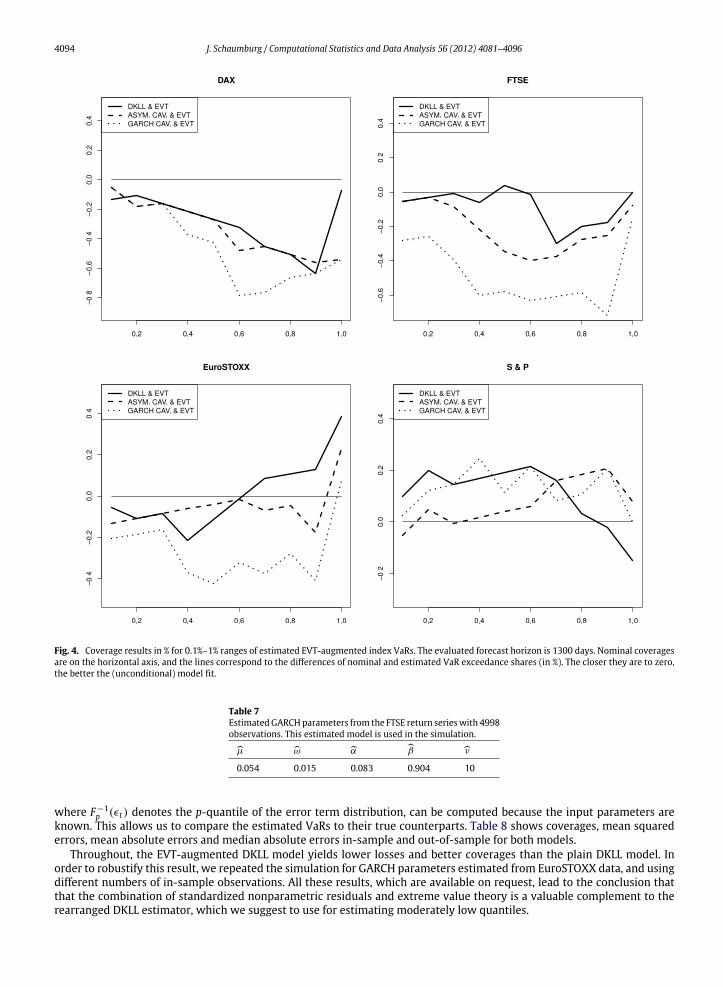
It was pointed out in Kuester et al. (2006), that for comparison of VaR prediction strategies, the focus should not belimited to one or two probability levels, but one should take a range of quantiles into account when deciding which modelis the best.
We adapt their graphical representation of coverage accuracy in Fig. 4 for VaR levels between 0.1% and 1%. For the sakeof clarity, the AR-TGARCH CAViaR, which usually showed results that were similar to one of the other two CAViaR models,is not included in the graph. It turns out that the Asymmetric Slope CAViaR is the stronger competitor for the DKLL model,as in three out of four cases, the lines corresponding to its differences to the nominal coverages are closer to zero than thosecorresponding to the GARCH CAViaR. In some ranges, e.g. 0.1%–0.5% FTSE VaR, the DKLL model clearly yields a very good fit.In other cases, such as DAX, all three models do not hit the correct coverages. The DKLL estimator, however, goes head tohead with the CAViaR models, while sometimes even beating them.
6. Simulation: Comparing DKLL and EVT-refined VaR
This section is devoted to the question of whether it is sensible to refine the nonparametric VaR estimator with extremevalue methods, instead of using the plain version even for extreme VaR estimation. One would expect that especially forsmall data sets, the EVT extrapolation into the far tails of return distributions yields more stable results than estimating thetail quantiles directly. In order to check this, we carry out a small simulation study to complement the empirical results fromthe previous sections. As the goal is to assess the relative accuracies of DKLL and EVT-refined DKLL estimators, we do notadditionally include the CAViaR models.
To the FTSE time series, we fit a GARCH(1, 1) model with t-distributed error terms. It has the following form:
Yt = µ + σtϵt , σ 2t = ω + αϵ2
t−1 + βσ 2t−1, ϵt ∼ tν . (6.1)
Parameter estimates are listed in Table 7.From the estimated model, a time series of 13000 observations is simulated. To obtain a setup which is realistic with
respect to usual data availability, only 2000 observations are used to estimate the models, and 0.1% VaR predictions arecomputed over two forecast horizons, N=5000 and N=10000. The advantages of simulated data are that they allow for muchlonger horizons, and that the return quantile functions
qtp = σtF−1p (ϵt),
4094 J. Schaumburg / Computational Statistics and Data Analysis 56 (2012) 4081–4096
Fig. 4. Coverage results in % for 0.1%–1% ranges of estimated EVT-augmented index VaRs. The evaluated forecast horizon is 1300 days. Nominal coveragesare on the horizontal axis, and the lines correspond to the differences of nominal and estimated VaR exceedance shares (in %). The closer they are to zero,the better the (unconditional) model fit.
Table 7EstimatedGARCHparameters from the FTSE return serieswith 4998observations. This estimated model is used in the simulation.µ ω α β ν0.054 0.015 0.083 0.904 10
where F−1p (ϵt) denotes the p-quantile of the error term distribution, can be computed because the input parameters are
known. This allows us to compare the estimated VaRs to their true counterparts. Table 8 shows coverages, mean squarederrors, mean absolute errors and median absolute errors in-sample and out-of-sample for both models.
Throughout, the EVT-augmented DKLL model yields lower losses and better coverages than the plain DKLL model. Inorder to robustify this result, we repeated the simulation for GARCH parameters estimated from EuroSTOXX data, and usingdifferent numbers of in-sample observations. All these results, which are available on request, lead to the conclusion thatthat the combination of standardized nonparametric residuals and extreme value theory is a valuable complement to therearranged DKLL estimator, which we suggest to use for estimating moderately low quantiles.

J. Schaumburg / Computational Statistics and Data Analysis 56 (2012) 4081–4096 4095
Table 8Coverages and different loss functions from comparing the estimated 0.1% VaRs with thetrue quantile function. Cov. stands for coverage, MSE for mean squared error, MAE for meanabsolute error and Med. AE for median absolute error.
In-sample: n=2000Cov. MSE MAE Med.AE
DKLL 0.001 1.049 0.753 0.52EVT-DKLL 0.001 0.605 0.579 0.429
Out-of-sample: N=5000Cov. MSE MAE Med.AE
DKLL 0.009 3.673 1.359 0.9EVT-DKLL 0.003 2.455 1.067 0.649
Out-of-sample: N=10000Cov. MSE MAE Med.AE
DKLL 0.008 3.379 1.253 0.787EVT-DKLL 0.004 2.281 0.981 0.578
7. Conclusion
In this paper, we propose a way to estimate and predict conditional Value at Risk from a nonparametric model. Weconsider probabilities that are of practical interest for financial institutions. For external market risk reporting, 1% portfolioVaRs have to be estimated on a daily basis. Internal risk management sometimes requires to take even more extremeprobabilities, such as 0.1%, into account. Although typically very few observations are available in the extreme tails, modelsto be used should be flexible and rest upon as few structural assumptions as possible. We suggest to use nonparametricquantile regression, more specifically, a rearranged Double Kernel Local Linear VaR estimator as well as a version of thelatter augmented by extreme value theory. Both are applied to different index return time series. Forecast performancesare benchmarked against the widely used CAViaR models. Although these also perform well in many occasions, none of theconsidered specifications systematically dominates the others. In contrast to them, nonparametric regression circumventsthe issue of choosing the appropriate parametrization.
Backtesting results from the evaluation of real as well as simulated data examples lead to the conclusion that the fullynonparametric and the EVT-refinednonparametricmodels not only outperform theparametric alternatives in a considerablenumber of situations, but that they can be used to predict VaR of any probability level of interest, even when the estimationperiod is ofmoderate size. In recent years, computing power has increased to such an extent that fully nonparametricmodelscome at little more computation cost than other models that rely on more restrictive assumptions. From the results inthis paper, however, we conclude that the gains on the additional flexibility are substantial and nonparametric quantileregression with EVT refinements should be considered as a practical alternative for estimating and forecasting VaR.
Acknowledgments
I would like to thank Melanie Schienle and Nikolaus Hautsch for their instructive and helpful comments on this project.The support from theDeutsche Forschungsgemeinschaft via SFB 649 ‘Ökonomisches Risiko’, Humboldt-Universität zu Berlin,is gratefully acknowledged.
References
Balkema, A.A., de Haan, L., 1974. Residual life time at great age. The Annals of Probability 2, 792–804.Cai, Z., 2002. Regression quantiles for time series. Econometric Theory 18, 169–192.Cai, Z., Wang, X., 2008. Nonparametric estimation of conditional var and expected shortfall. Journal of Econometrics 147, 120–130.Chen, S.X., Tang, C.Y., 2005. Nonparametric inference of value-at-risk for dependent financial returns. Journal of Financial Econometrics 3, 227–255.Chernozhukov, V., Fernandez-Val, I., Galichon, A., 2009. Improving point and interval estimates of monotone functions by rearrangement. Biometrika 96,
559–575.Chernozhukov, V., Umantsev, L., 2001. Conditional value-at-risk: aspects of modelling and estimation. Empirical Economics 26, 271–292.Dette, H., Neumeyer, N., Pilz, K.F., 2006. A simple nonparametric estimator of a strictly monotone regression function. Bernoulli 12, 469–490.Drees, H., 2003. Extreme quantile estimation for dependent data, with applications to finance. Bernoulli 9, 617–657.El-Arouia, M.-A., Diebolt, J., 2002. On the use of the peaks over thresholds method for estimating out-of-sample quantiles. Computational Statistics and
Data Analysis 39, 453–475.Embrechts, P., Klüppelberg, C., Mikosch, T., 1997. Modelling Extremal Events. Springer.Engle, R.F., Manganelli, S., 2004. Caviar: conditional autoregressive value at risk by regression quantiles. Journal of Business & Economic Statistics 22,
367–381.Fan, J., Gijbels, I., 1996. Local Polynomial Modelling and its Applications. In: Monographs on Statistics and Applied Probability, vol. 66. Chapman & Hall.Koenker, R., Bassett, G., 1978. Regression quantiles. Econometrica 46, 33–50.Koenker, R., Zhao, Q., 1996. Conditional quantile estimation and inference for arch models. Econometric Theory 12, 793–813.Kuester, K., Mittnik, S., Paolella, M.S., 2006. Value-at-risk prediction: a comparison of alternative strategies. Journal of Financial Econometrics 4, 53–89.Kupiec, P.H., 1995. Techniques for verifying the accuracy of risk measurement models. Journal of Derivatives 73–84.

4096 J. Schaumburg / Computational Statistics and Data Analysis 56 (2012) 4081–4096
Li, Q., Racine, J.S., 2007. Nonparametric Econometrics. Princeton University Press.MacDonald, A., Scarrott, C., Lee, D., Darlowb, B., Reale, M., Russell, G., 2011. A flexible extreme value mixture model. Computational Statistics and Data
Analysis 55, 2137–2157.Manganelli, S., Engle, R.F., 2001. Value at risk models in finance. In: ECB Working Paper Series Working Paper No. 75.McNeil, A., Frey, R., 2000. Estimation of tail-related risk measures for heteroscedastic financial time series: an extreme value approach. Journal of Empirical
Finance 7, 271–300.McNeil, A.J., Frey, R., Embrechts, P., 2005. Quantitative Risk Management: Concepts, Techniques and Tools. Princeton University Press.Nieto, M.R., Ruiz, E., 2008. Measuring financial risk: comparison of alternative procedures to measure var and es. In: Universidad Carlos III de Madrid
Working Paper No. 08-73.Pickands, J., 1975. Statistical inference using extreme order statistics. The Annals of Statistics 3, 119–131.Smith, R.L., 1987. Estimating the tails of probability distributions. The Annals of Statistics 15, 1174–1207.Taylor, J.W., 2008. Using exponentially weighted quantile regression to estimate value at risk and expected shortfall. Journal of Financial Econometrics 6,
382–406.Wu, W.B., Yu, K., Mitra, G., 2007. Kernel conditional quantile estimation for stationary processes with application to value at risk. Journal of Financial
Econometrics 1–18.Yu, K., Jones, M., 1997. A comparison of local constant and local linear regression quantile estimators. Computational Statistics and Data Analysis 25,
159–166.Yu, K., Jones, M.C., 1998. Local linear quantile regression. Journal of the American Statistical Association 93, 228–237.