J.Stat.M

ech.(2009)

P01005

ournal of Statistical Mechanics:An IOP and SISSA journalJ Theory and Experiment

Predicting extinction rates in stochasticepidemic models

Ira B Schwartz1, Lora Billings2, Mark Dykman3 andAlexandra Landsman4

1 US Naval Research Laboratory, Code 6792, Nonlinear Systems DynamicsSection, Plasma Physics Division, Washington, DC 20375, USA2 Department of Mathematical Sciences, Montclair State University, Montclair,NJ 07043, USA3 Department of Physics and Astronomy, Michigan State University,East Lansing, MI 48824, USA4 Department of Physics and Astronomy, James Madison University,Harrisonburg, VA 22807, USAE-mail: ira.schwartz@nrl.navy.mil, billingsl@mail.montclair.edu,dykman@pa.msu.edu and landsmax@jmu.edu

Received 27 June 2008Accepted 17 September 2008Published 5 January 2009

Online at stacks.iop.org/JSTAT/2009/P01005doi:10.1088/1742-5468/2009/01/P01005

Abstract. We investigate the stochastic extinction processes in a class ofepidemic models. Motivated by the process of natural disease extinction inepidemics, we examine the rate of extinction as a function of disease spread. Weshow that the effective entropic barrier for extinction in a susceptible–infected–susceptible epidemic model displays scaling with the distance to the bifurcationpoint, with an unusual critical exponent. We make a direct comparison betweenpredictions and numerical simulations. We also consider the effect of non-Gaussian vaccine schedules, and show numerically how the extinction processmay be enhanced when the vaccine schedules are Poisson distributed.

Keywords: fluctuations (theory), stochastic processes (theory), populationdynamics (theory)

c©2009 IOP Publishing Ltd and SISSA 1742-5468/09/P01005+12$30.00

J.Stat.M

ech.(2009)

P01005

Predicting extinction rates in stochastic epidemic models

Contents

1. Introduction 2

2. The discrete model 3

3. Disease extinction 4

4. Numerical simulations 6

5. Conclusions and discussion 8

Acknowledgments 10

Appendix A 10

Appendix B 11

References 11

1. Introduction

One of the major goals of the studies of stochastic population dynamics, especiallyin modeling epidemic spread in a population, is that of predicting finite extinctiontimes when one or more components of the population goes to zero. Practically alldiseases of interest exhibit randomness resulting in observed fluctuations. Childhooddiseases [1]–[3], meningitis [4], dengue fever and malaria [5] are but a few examples whereincidence rates fluctuate with significant amplitude. These fluctuations arise from randomcontacts within a population, uncertainty in epidemic parameters, and stochastic fluxchanges from external coupled populations [6, 7]. As diseases evolve in large populations,there is the possibility of finite time extinction and reintroduction of the disease [8, 9].Extinction occurs where the number of infectives becomes so small that there is insufficienttransmission to keep the disease in its endemic state [10]–[12]. Therefore, in the absenceof disease reintroduction, the epidemic dies out.

A common mathematical approach to modeling the dynamics of disease spread isto compartmentalize the population into susceptibles (S), infectives (I), and possiblyrecovered (R). Often it is assumed that there is strong mixing in the system, that is,all species interact with all species, and therefore the species densities do not depend onspatial coordinates. In these models, called SIS or SIR models [13], the disease spread canbe characterized by the reproductive rate of infection, R0. In its deterministic form, R0

can be defined so that, for an endemic state to exist along with the disease-free equilibrium(DFE), R0 > 1. When R0 < 1, the DFE is globally stable and the disease becomes extinct.For appropriate parameters where the two states coexist, the DFE is unstable and theendemic state is attracting. In the models we consider here, it is assumed that the endemicstate is globally attracting when R0 > 1.

In the presence of random fluctuations, the situation becomes more complicated.Fluctuations cause the disease-free state to be reached, albeit for a limited time, as

doi:10.1088/1742-5468/2009/01/P01005 2

J.Stat.M

ech.(2009)

P01005

Predicting extinction rates in stochastic epidemic models

indicated by both numerical [14]–[17] and analytic [18, 19, 13, 20, 21] results for variousmodels. Such an extinction process occurs even when R0 is greater than unity.

A major characteristic of fluctuation-induced extinction in the SIS stochastic modelfor large populations is the extinction rate, or the reciprocal mean first time the number ofinfectives approaches zero. It has been studied by approximating the full two-dimensionalstochastic system (or, more precisely, the system with two dynamical variables) as acontinuous one, with fluctuations induced by noise in the Langevin approach. Recently,Doering et al [21] investigated a discrete birth–death SIS model and compared it to acontinuous model. The analysis referred to a one-variable model, which allows one toobtain an explicit solution in various regimes of R0. However, this model does not revealsome generic features of the full discrete SIS system related to the lack of detailed balance.

It is the purpose of this paper to analyze the general SIS discrete model, and obtainexplicit scaling behavior of the extinction rate in the neighborhood of disease onset;i.e., when the reproductive rate is greater than but close to unity. To make clear theassumptions we use for the description of the extinction process, we will include thetheory presented in [27]. Using the scaling results, we will compare theory and numericalcomputations for the extinction rate exponents. Since disease extinction is a goal ofvaccine control, and vaccine scheduling is inherently random despite the best policycontrols, we numerically examine the case where the vaccine schedule is a Poisson process.A direct comparison between the non-vaccine and vaccine cases will be made numerically.

2. The discrete model

We consider a model where susceptibles (S) are born at rate μ, both susceptibles andinfectives (I) die at the same rate μ, and infectives recover at rate κ and immediatelybecome susceptible. If susceptibles contact infectives, they may become infected at rateβ. We follow and reproduce the model and notation given in [27].

Since the numbers of susceptibles S and infectives I are integers whereas the eventsof birth, death, and contact happen at random, we describe the process by the masterequation. We introduce vector X = (X1, X2) with components X1 = S, X2 = I and vectorr = (r1, r2) with integer components r1 and r2, which give, respectively, the incrementsin S and I in a single transition. The quantity of interest is the probability ρ(X, t) tohave given S and I at time t. If transitions are short and uncorrelated, X(t) is a Markovprocess, and the evolution of ρ(X, t) is described by the equation

ρ(X, t) =∑

r

[W (X− r; r)ρ(X− r, t) − W (X; r)ρ(X, t)] . (1)

In the absence of vaccination the transition rates W (X, r) are

W (X; (1, 0)) = Nμ, W (X; (−1, 0)) = μX1,

W (X; (0,−1)) = μX2, W (X; (1,−1)) = κX2,

W (X; (−1, 1)) = βX1X2/N,

(2)

where N is the scaling factor which we set equal to the average population, N � 1.For sufficiently large S, I ∝ N , fluctuations of S, I are small on average. If these

fluctuations are disregarded, one arrives at the deterministic (mean-field) equations for

doi:10.1088/1742-5468/2009/01/P01005 3

J.Stat.M

ech.(2009)

P01005

Predicting extinction rates in stochastic epidemic models

the mean values of S, I:

X1 = Nμ − μX1 + κX2 − βX1X2/N,

X2 = −(μ + κ)X2 + βX1X2/N.(3)

These are standard equations of the SIS model [1]. For R0 = β/(μ + κ) > 1 they havea stable solution XA = NxA with x1A = R−1

0 , x2A = 1 − R−10 . It describes the endemic

disease. In addition, (3) have an unstable stationary state (saddle point) XS = NxS withx1S = 1, x2S = 0. This state corresponds to extinction of infectives.

For N � 1, the steady state distribution ρ(X) has a peak at the stable stateXA with width ∝N1/2. This peak is formed over a typical relaxation time tr =max[μ−1, (β−μ−κ)−1], which is much smaller than the extinction time. We are interestedin the probability of having a small number infected, X2 � X2A. It is determined by thetail of the distribution. The tail can be approximated by seeking the solution of (1) inthe eikonal form,

ρ(X) = exp[−Ns(x)], x = X/N,

ρ(X + r) ≈ ρ(X) exp(−pr), p = ∂xs.(4)

For time independent parameters W this formulation was used in a number of papers [20]–[27]. The function s(x) gives the logarithm of the stationary distribution scaled by theaverage population, and is given by s = −H(x, ∂xs; t). The function s(x) is the effectiveaction, and H the auxiliary Hamiltonian.

Following the standard approach of classical mechanics, we can find the action s(x)from classical trajectories of the auxiliary system,

H(x,p; t) = μ(ep1 − 1) + μx1(e−p1 − 1) + μx2(e

−p2 − 1)

+ κx2(ep1−p2 − 1) + βx1x2(e

p2−p1 − 1) (5)

that satisfy equations

x = ∂pH(x,p; t), p = −∂xH(x,p; t). (6)

3. Disease extinction

In this section we analyze the stationary distribution using the eikonal approximationdeveloped in the previous section for the case where fluctuations are from random contacts.We begin by noting that H = 0, which in turn is a consequence of the condition ∂ts = 0.The function s(x) has the form [25, 27],

s(xf ) =

∫ tf

−∞p x dt, H(x,p) = 0. (7)

Here, the integral is calculated for a Hamiltonian trajectory (x(t),p(t)) that starts att → −∞ at x → xA,p → 0 and arrives at time tf at a state xf . The correspondingtrajectory describes the most probable sequence of elementary events X → X+r bringingthe system to Nxf . It provides the absolute minimum to s(xf ), and s(xf ) is independentof tf . The quantity Ns(x) gives the exponent in the expression for the mean first-passagetime for reaching Nx from the vicinity of the attractor XA [28].

doi:10.1088/1742-5468/2009/01/P01005 4

J.Stat.M

ech.(2009)

P01005

Predicting extinction rates in stochastic epidemic models

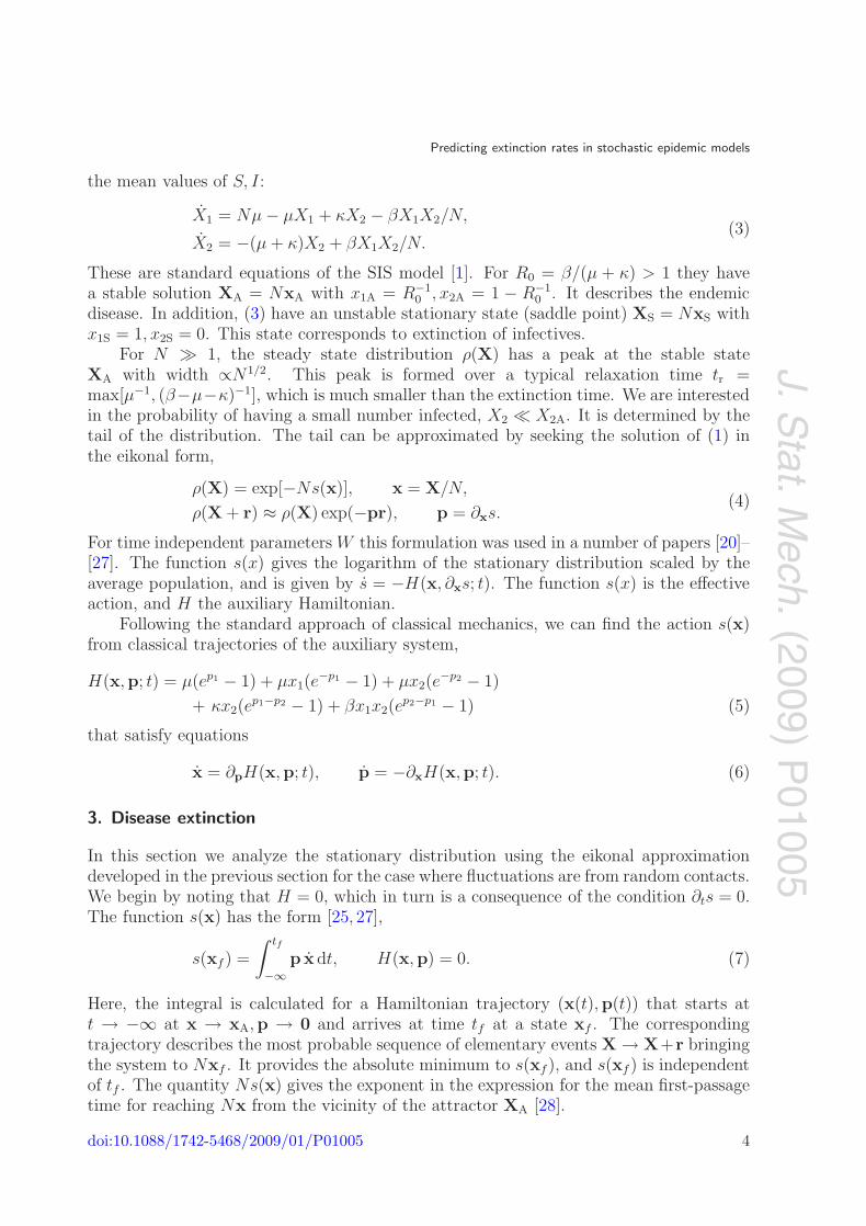
Figure 1. 3D projections of the optimal extinction trajectory in (6) and (B.2) inscaled coordinates x2 = x2/(R0−1), p2 = p2/(R0−1), x′

1 = (1−x1)/(R0−1), p1 =(μ/β)(R0 − 1)2p1. Panels (a) and (b) show x1, x2, p1 and x1, x2, p2 projections.The trajectory goes from point A that corresponds to the stable state of thesystem with coordinates xA and zero momentum to point S that corresponds toextinction of the disease, with coordinate xS and with non-zero momentum p.

From equation (4), the extinction rate is determined by s calculated for x2 → 0, i.e.,by the probability density for reaching the disease-free state. It is easy to see that theminimum of s(x) over x1 for x2 → 0 is reached at the saddle point xS of the fluctuation-free motion. Thus the entropic barrier for extinction is Nsext = Ns(xS), and the typicalextinction time is τ ∝ exp(Nsext).

The Hamiltonian trajectory xext(t),pext(t) that gives s(xA) is the optimal extinctiontrajectory. One can show that it approaches xA as t → ∞. This is similar to otherproblems of an optimal trajectory leading from a deterministic stable state to a saddlepoint [25, 29]. However, in contrast to the more common situation, for t → ∞ themomentum pext does not go to zero. Instead pext(t) → pS, with pS = (0,− lnR0).This is in spite of the fact that, along with (xS,pS), the Hamiltonian H has a ‘standard’fixed point (xS,p = 0). A proof is given in appendix A.

An explicit analytical solution for the Hamiltonian trajectories can be obtained closeto a bifurcation point where the number of the stationary solutions of the deterministicequations changes [25, 27]. In the present case it corresponds to 0 < η � 1, η = β−μ−κ ≡β(R0 − 1)/R0. For η � 1 the mean-field value of x2 in the stable state x2A = η/β � 1is close to x2S . The relaxation time of x2 near the stable state is η−1. It is much longerthan the relaxation time of x1, which is μ−1, i.e., x2 is a soft mode. Coordinate x1 followsx2 adiabatically on the timescale that largely exceeds μ−1. See appendix B for details.

The solution (B.2) in appendix B describes in particular the optimal extinctiontrajectory as depicted in figure 1. The full Hamiltonian equations (5) and (6) were alsosolved numerically to get the optimal path from the attractor to the extinct state. Thesolution is compared with the adiabatic solution in figure 2, where the control parameter,η, is small.

doi:10.1088/1742-5468/2009/01/P01005 5

J.Stat.M

ech.(2009)

P01005

Predicting extinction rates in stochastic epidemic models

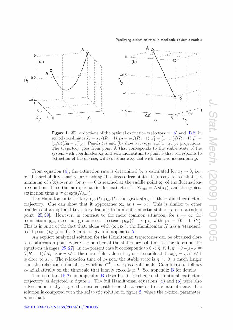
Figure 2. Time series of the heteroclinic orbits. The time series in bold representsthose of the adiabatic equations in (B.2). The dashed lines were computed usingthe full Hamiltonian system (6), where time was scaled to the period of a longperiod approximating orbit to the heteroclinic orbit. The parameter values inthe numerical computations were μ = 0.02, κ = 100.0, β = 100.05, η = 0.0308.

From (7) and (B.2), we derive one of our main results,

sext = s(xS) = η2/2β2 = (R0 − 1)2/2R20. (8)

The entropic barrier for extinction Nsext scales with the distance to the bifurcation pointη ∝ R0 − 1 as η2. This is in contrast to the case for standard scaling of the activationenergy of escape near a saddle–node bifurcation point, where the critical exponent is3/2 [25]. Such unusual scaling is related to pS being non-zero. It emerges also in the SIRmodel [30].

4. Numerical simulations

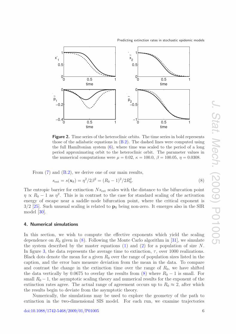
In this section, we wish to compute the effective exponents which yield the scalingdependence on R0 given in (8). Following the Monte Carlo algorithm in [31], we simulatethe system described by the master equations (1) and (2) for a population of size N .In figure 3, the data represents the average time to extinction, τ , over 1000 realizations.Black dots denote the mean for a given R0 over the range of population sizes listed in thecaption, and the error bars measure deviation from the mean in the data. To compareand contrast the change in the extinction time over the range of R0, we have shiftedthe data vertically by 0.0675 to overlay the results from (8) where R0 − 1 is small. Forsmall R0 − 1, the asymptotic scaling theory and numerical results for the exponent of theextinction rates agree. The actual range of agreement occurs up to R0 ≈ 2, after whichthe results begin to deviate from the asymptotic theory.

Numerically, the simulations may be used to explore the geometry of the path toextinction in the two-dimensional SIS model. For each run, we examine trajectories

doi:10.1088/1742-5468/2009/01/P01005 6

J.Stat.M

ech.(2009)

P01005

Predicting extinction rates in stochastic epidemic models

Figure 3. The logarithm of the extinction time τ scaled by the population size, N .Black dots are the average over N of log(τ). The dashed line is the extrapolationof equation (8). The fixed parameters are: μ = 0.02 (1/year), κ = 100 (1/year),and N = 20, 30, 40, 50, 60, 70, 80 (people). We vary β to adjust R0.

Figure 4. A pre-history histogram plot in the state space of (S, I). The endemicstate is represented by the star, while the filled circle locates the DFE. Thegrayscale denotes the number of points that occur at a given discrete value of(S, I) over 5000 realizations. The segment of the optimal path to extinctioncan be seen along the peak of the distribution. Parameters: μ = 0.02 (1/year),β = 110 (1/year), κ = 100 (1/year), and N = 1000 (people).

leading to extinction at the DFE. We then reverse time along the orbit until we reach aneighborhood of the endemic state. In figure 4, a plot is shown of the averaged pre-historyrealizations projected onto (S, I) state space. Notice in the figure that the peak of thedistribution lies along a curve approximating the optimal path segment from the endemicstate to the DFE, given by the adiabatic approximation in normalized coordinates asx2 = 1 − x1.

doi:10.1088/1742-5468/2009/01/P01005 7

J.Stat.M

ech.(2009)

P01005

Predicting extinction rates in stochastic epidemic models

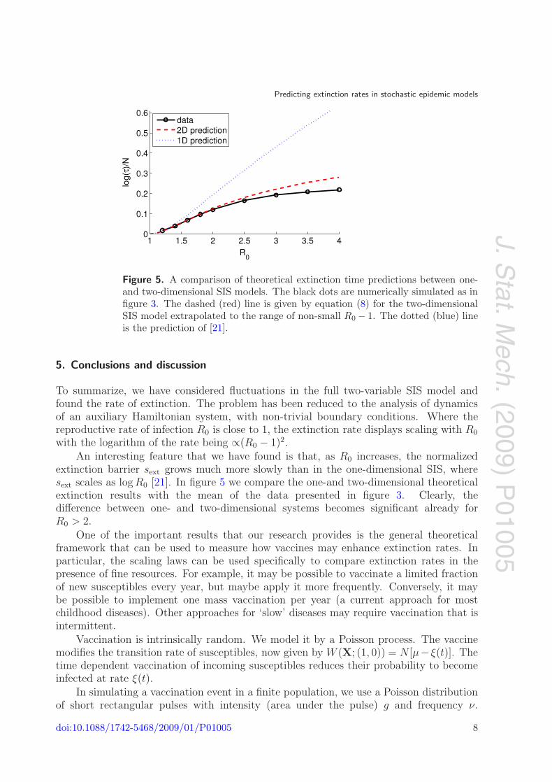
Figure 5. A comparison of theoretical extinction time predictions between one-and two-dimensional SIS models. The black dots are numerically simulated as infigure 3. The dashed (red) line is given by equation (8) for the two-dimensionalSIS model extrapolated to the range of non-small R0 − 1. The dotted (blue) lineis the prediction of [21].

5. Conclusions and discussion

To summarize, we have considered fluctuations in the full two-variable SIS model andfound the rate of extinction. The problem has been reduced to the analysis of dynamicsof an auxiliary Hamiltonian system, with non-trivial boundary conditions. Where thereproductive rate of infection R0 is close to 1, the extinction rate displays scaling with R0

with the logarithm of the rate being ∝(R0 − 1)2.An interesting feature that we have found is that, as R0 increases, the normalized

extinction barrier sext grows much more slowly than in the one-dimensional SIS, wheresext scales as log R0 [21]. In figure 5 we compare the one-and two-dimensional theoreticalextinction results with the mean of the data presented in figure 3. Clearly, thedifference between one- and two-dimensional systems becomes significant already forR0 > 2.

One of the important results that our research provides is the general theoreticalframework that can be used to measure how vaccines may enhance extinction rates. Inparticular, the scaling laws can be used specifically to compare extinction rates in thepresence of fine resources. For example, it may be possible to vaccinate a limited fractionof new susceptibles every year, but maybe apply it more frequently. Conversely, it maybe possible to implement one mass vaccination per year (a current approach for mostchildhood diseases). Other approaches for ‘slow’ diseases may require vaccination that isintermittent.

Vaccination is intrinsically random. We model it by a Poisson process. The vaccinemodifies the transition rate of susceptibles, now given by W (X; (1, 0)) = N [μ− ξ(t)]. Thetime dependent vaccination of incoming susceptibles reduces their probability to becomeinfected at rate ξ(t).

In simulating a vaccination event in a finite population, we use a Poisson distributionof short rectangular pulses with intensity (area under the pulse) g and frequency ν.

doi:10.1088/1742-5468/2009/01/P01005 8

J.Stat.M

ech.(2009)

P01005

Predicting extinction rates in stochastic epidemic models

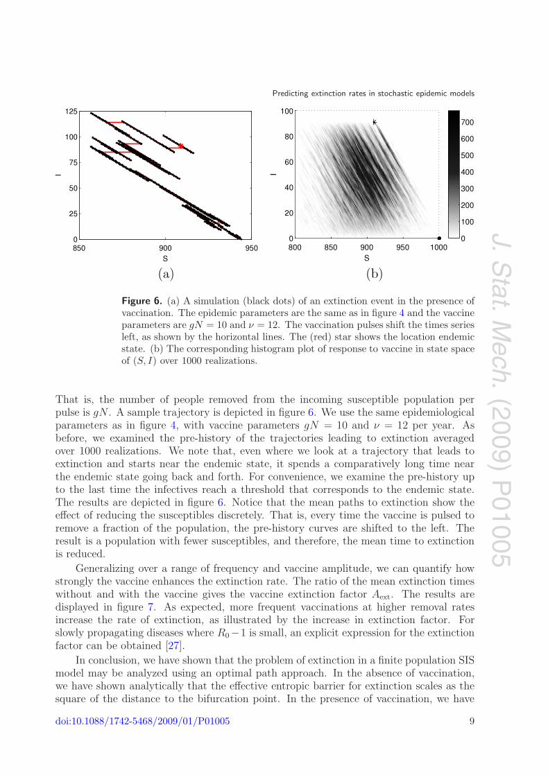
Figure 6. (a) A simulation (black dots) of an extinction event in the presence ofvaccination. The epidemic parameters are the same as in figure 4 and the vaccineparameters are gN = 10 and ν = 12. The vaccination pulses shift the times seriesleft, as shown by the horizontal lines. The (red) star shows the location endemicstate. (b) The corresponding histogram plot of response to vaccine in state spaceof (S, I) over 1000 realizations.

That is, the number of people removed from the incoming susceptible population perpulse is gN . A sample trajectory is depicted in figure 6. We use the same epidemiologicalparameters as in figure 4, with vaccine parameters gN = 10 and ν = 12 per year. Asbefore, we examined the pre-history of the trajectories leading to extinction averagedover 1000 realizations. We note that, even where we look at a trajectory that leads toextinction and starts near the endemic state, it spends a comparatively long time nearthe endemic state going back and forth. For convenience, we examine the pre-history upto the last time the infectives reach a threshold that corresponds to the endemic state.The results are depicted in figure 6. Notice that the mean paths to extinction show theeffect of reducing the susceptibles discretely. That is, every time the vaccine is pulsed toremove a fraction of the population, the pre-history curves are shifted to the left. Theresult is a population with fewer susceptibles, and therefore, the mean time to extinctionis reduced.

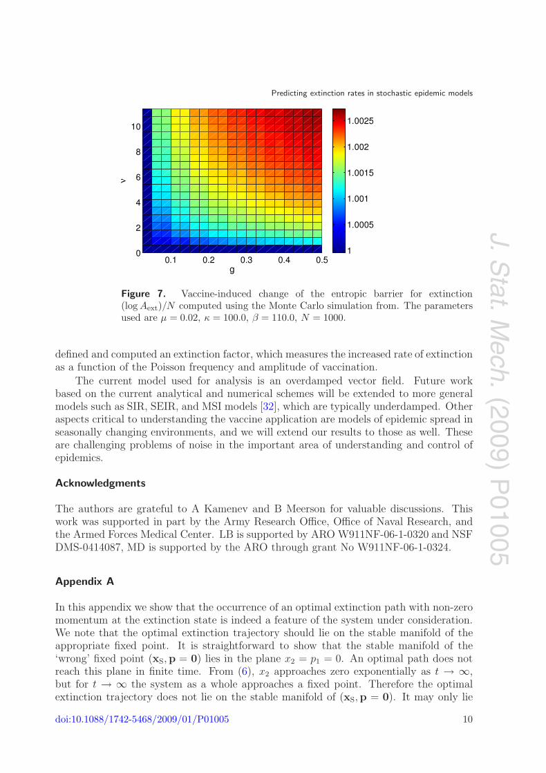
Generalizing over a range of frequency and vaccine amplitude, we can quantify howstrongly the vaccine enhances the extinction rate. The ratio of the mean extinction timeswithout and with the vaccine gives the vaccine extinction factor Aext. The results aredisplayed in figure 7. As expected, more frequent vaccinations at higher removal ratesincrease the rate of extinction, as illustrated by the increase in extinction factor. Forslowly propagating diseases where R0−1 is small, an explicit expression for the extinctionfactor can be obtained [27].

In conclusion, we have shown that the problem of extinction in a finite population SISmodel may be analyzed using an optimal path approach. In the absence of vaccination,we have shown analytically that the effective entropic barrier for extinction scales as thesquare of the distance to the bifurcation point. In the presence of vaccination, we have

doi:10.1088/1742-5468/2009/01/P01005 9

J.Stat.M

ech.(2009)

P01005

Predicting extinction rates in stochastic epidemic models

Figure 7. Vaccine-induced change of the entropic barrier for extinction(log Aext)/N computed using the Monte Carlo simulation from. The parametersused are μ = 0.02, κ = 100.0, β = 110.0, N = 1000.

defined and computed an extinction factor, which measures the increased rate of extinctionas a function of the Poisson frequency and amplitude of vaccination.

The current model used for analysis is an overdamped vector field. Future workbased on the current analytical and numerical schemes will be extended to more generalmodels such as SIR, SEIR, and MSI models [32], which are typically underdamped. Otheraspects critical to understanding the vaccine application are models of epidemic spread inseasonally changing environments, and we will extend our results to those as well. Theseare challenging problems of noise in the important area of understanding and control ofepidemics.

Acknowledgments

The authors are grateful to A Kamenev and B Meerson for valuable discussions. Thiswork was supported in part by the Army Research Office, Office of Naval Research, andthe Armed Forces Medical Center. LB is supported by ARO W911NF-06-1-0320 and NSFDMS-0414087, MD is supported by the ARO through grant No W911NF-06-1-0324.

Appendix A

In this appendix we show that the occurrence of an optimal extinction path with non-zeromomentum at the extinction state is indeed a feature of the system under consideration.We note that the optimal extinction trajectory should lie on the stable manifold of theappropriate fixed point. It is straightforward to show that the stable manifold of the‘wrong’ fixed point (xS,p = 0) lies in the plane x2 = p1 = 0. An optimal path does notreach this plane in finite time. From (6), x2 approaches zero exponentially as t → ∞,but for t → ∞ the system as a whole approaches a fixed point. Therefore the optimalextinction trajectory does not lie on the stable manifold of (xS,p = 0). It may only lie

doi:10.1088/1742-5468/2009/01/P01005 10

J.Stat.M

ech.(2009)P

01005

Predicting extinction rates in stochastic epidemic models

on the stable manifold of the fixed point (xS,pS), which is not confined to a plane in the(x,p) space. An alternative argument is provided in [27].

The situation where an auxiliary Hamiltonian system has two fixed points with thesame xS was first noticed for a system described by the Fokker–Planck equation witha singular diffusion matrix at xS [18], and the ‘right’ point was chosen on the basis ofnumerical simulations. This situation was also found for a system described by a one-variable master equation, where the Hamiltonian dynamics is integrable [20]; it occursalso in a two-variable susceptible–infected–recovered (SIR) model concurrently studied byKamenev and Meerson [30].

Appendix B

The solution of Hamiltonian equations (6) in the adiabatic approximation is simplified bythe fact that x2 � 1 and |p2| � 1. To leading order in η we have x1 = 1−x2, p1 = βx2p2/μ,while the equations for slow variables x2, p2 have the Hamiltonian form

x2 = ∂Had/∂p2, p2 = −∂Had/∂x2, (B.1)

with Hamiltonian Had = ηx2p2 − βx2p2(x2 − p2). The Hamiltonian trajectory is

p2(t) = x2(t) − η

β, x2(t) = x2A

(1 + eη(t−t0)

)−1. (B.2)

References

[1] Anderson R M and May R M, 1991 Infectious Diseases of Humans—Dynamics and Control (Oxford:Oxford Science Publications)

[2] Bolker B M and Grenfell B T, Chaos and biological complexity in measles dynamics, 1993 Proc. R. Soc.Lond. B 251 75

[3] Bolker B M, Chaos and complexity in measles models—a comparative numerical study , 1993 IMA J. Math.Appl. Med. 10 83

[4] Patz J, A human disease indicator for the effects recent global climate change, 2002 Proc. Nat. Acad. Sci.99 12506

[5] Patz J, Hulme M, Rosenzweig C, Mitchell T, Goldberg R, Githeko A, Lele S, McMichael A andLe Sueur D, Climate change: regional warming and malaria resurgence, 2002 Nature 420 627

[6] Rand D A and Wilson H B, Chaotic stochasticity: a ubiquitous source of unpredictability in epidemics, 1991Proc. R. Soc. Lond. B 246 179

[7] Billings L, Bollt E M and Schwartz I B, Phase-space transport of stochastic chaos in population dynamics ofvirus spread , 2002 Phys. Rev. Lett. 88 234101

[8] Andersson H and Britton T, Stochastic epidemics in dynamic populations: quasi-stationarity andextinction, 2000 J. Math. Biol. 41 559

[9] Cummings D A T, Irizarry R A, Huang N E, Endy T P, Nisalak A, Ungchusak K and Burke D S,Travelling waves in the occurrence of dengue haemorrhagic fever in Thailand , 2004 Nature 427 344

[10] Keeling M J, 2004 Ecology, Genetics, and Evolution (New York: Elsevier)[11] Verdasca J A, da Gama M M T, Nunes A and Bernardino N R, Recurrent epidemics in small world

networks, 2005 J. Theor. Biol. 233 553[12] Bartlett M S, Some evolutionary stochastic processes, 1949 J. R. Statist. Soc. B 11 211[13] Jacquez J A and Simon C P, The stochastic si model with recruitment and deaths. 1. Comparison with the

closed sis model , 1993 Math. Biosci. 117 77[14] West R W and Thompson J R, Models for the simple epidemic, 1997 Math. Biosci. 141 29[15] Nasell I, On the quasi-stationary distribution of the stochastic logistic epidemic, 1999 Math. Biosci. 156 21[16] Billings L and Schwartz I B, A unified prediction of computer virus spread in connected networks, 2002

Phys. Lett. A 297 261

doi:10.1088/1742-5468/2009/01/P01005 11

J.Stat.M

ech.(2009)

P01005

Predicting extinction rates in stochastic epidemic models

[17] Cummings D A T, Schwartz I B, Billings L, Shaw L B and Burke D S, Dynamic effects ofantibody-dependent enhancement on the fitness of viruses, 2005 Proc. Nat. Acad. Sci. 102 15259

[18] van Herwaarden O A and Grasman J, Stochastic epidemics, major outbreaks and the duration of theendemic period , 1995 J. Math. Biol. 33 581

[19] Allen L J S and Burgin A M, Comparison of deterministic and stochastic sis and sir models in discretetime, 2000 Math. Biosci. 163 1

[20] Elgart V and Kamenev A, Rare event statistics in reaction–diffusion systems, 2004 Phys. Rev. E 70 041106[21] Doering C R, Sargsyan K V and Sander L M, Extinction times for birth–death processes: exact results,

continuum asymptotics, and the failure of the Fokker–Planck approximation, 2005 Multiscale ModelingSimul. 3 283

[22] Kubo R, Matsuo K and Kitahara K, Fluctuation and relaxation of macrovariables, 1973 J. Stat. Phys. 9 51[23] Ventcel’ A D, Rough limit theorems on large deviations for Markov random processes. I , 1976 Teor.

Verojatn. Primen. 21 235[24] Hu G, Stationary solution of master-equations in the large-system-size limit, 1987 Phys. Rev. A 36 5782[25] Dykman M I, Mori E, Ross J and Hunt P M, Large fluctuations and optimal paths in chemical-kinetics,

1994 J. Chem. Phys. 100 5735[26] Tretiakov O A, Gramespacher T and Matveev K A, Lifetime of metastable states in resonant tunneling

structures, 2003 Phys. Rev. B 67 073303[27] Dykman M I, Schwartz I B and Landsman A, Disease extinction in the presence of non-Gaussian noise,

2008 Phys. Rev. Lett. 101 078101[28] Matkowsky B J, Schuss Z, Knessl C, Tier C and Mangel M, Asymptotic solution of the Kramers–Moyal

equation and first-passage times for markov jump processes, 1984 Phys. Rev. A 29 3359[29] Maier R S and Stein D L, Limiting exit location distributions in the stochastic exit problem, 1997 SIAM J.

Appl. Math. 57 752[30] Kamenev A and Meerson B, Extinction of the infectious disease: a large fluctuation in a nonequilibrium

system, 2008 Phys. Rev. E 77 061107[31] Gillespie D T, Exact stochastic simulation of coupled chemical-reactions, 1977 Papers of the American

Chemical Society vol 173 p 128 (Abstract)[32] Billings L and Schwartz I B, Exciting chaos with noise: unexpected dynamics in epidemic outbreaks, 2002

J. Math. Biol. 44 31

doi:10.1088/1742-5468/2009/01/P01005 12