© 2012 ISIJ 1054

ISIJ International, Vol. 52 (2012), No. 6, pp. 1054–1065

Predicting Delta Ferrite Content in Stainless Steel Castings

Marcelo Aquino MARTORANO,1)* Caio Fazzioli TAVARES2) and Angelo Fernando PADILHA1)

1) University of São Paulo, Department of Metallurgical and Materials Engineering, Av. Prof. Mello Moraes, 2463, São Paulo,SP, CEP 05508-900 Brasil. E-mail: martoran@usp.br, padilha@usp.br2) Açotécnica S.A., Via de Acesso João de Góes, 1900, Jandira, SP, CEP 06612-912 Brasil. E-mail: fazzioli@yahoo.com

(Received on October 28, 2011; accepted on February 7, 2012)

The distribution of delta ferrite fraction was measured with the magnetic method in specimens of dif-ferent stainless steel compositions cast by the investment casting (lost wax) process. Ferrite fraction mea-surements published in the literature for stainless steel cast samples were added to the present workdata, enabling an extensive analysis about practical methods to calculate delta ferrite fractions in stainlesssteel castings. Nineteen different versions of practical methods were formed using Schaeffler, DeLong,and Siewert diagrams and the nickel and chromium equivalent indexes suggested by several authors.These methods were evaluated by a detailed statistical analysis, showing that the Siewert diagram, includ-ing its equivalent indexes and iso-ferrite lines, gives the lowest relative errors between calculated andmeasured delta ferrite fractions. Although originally created for stainless steel welds, this diagram givesrelative errors lower than those for the current ASTM standard method (800/A 800M-01), developed topredict ferrite fractions in stainless steel castings. Practical methods originated from a combination of dif-ferent chromium/nickel equivalent indexes and the iso-ferrite lines from Schaeffler diagram give the lowestrelative errors when compared with combinations using other iso-ferrite line diagrams. For the samplescast in the present work, an increase in cooling rate from 0.78 to 2.7 K/s caused a decrease in the deltaferrite fraction, but a statistical hypothesis test revealed that this effect is significant in only 50% of thesamples that have ferrite in their microstructures.

KEY WORDS: stainless steel; casting; phase transformation; ferrite.

1. Introduction

Austenitic stainless steels have numerous applicationsdue to a good combination of properties, such as, corrosionand oxidation resistance, toughness, weldability, andmechanical strength at low and high temperatures. Stainlesssteel properties and performance are strongly related to itsmicrostructure, especially the amount and distribution ofdelta ferrite. In the case of castings and welds, these dependchiefly on chemical composition and on the cooling rateduring and after solidification.1) Phase diagrams are impor-tant to predict the type and amount of phases present instainless steel microstructures, but they are hardly availablefor steel compositions with more than five components,which is frequently the case in industrial applications.Therefore, practical methods based on empirical maps thatindicate the amount and types of phases in the microstruc-ture as a function of alloy chemical composition have beendeveloped.2) Schaeffler3) was one of the first to propose anempirical diagram in which alloying elements were dividedinto two groups: austenite and ferrite stabilizers. Formulaswere developed to calculate two indexes, namely a nickelequivalent (Nieq) and a chromium equivalent (Creq), whichquantified the effects of the austenite and ferrite stabilizers,respectively. General expressions for the Nieq and Creq usedby several authors are given below

... (1)

.......................................... (2)

where AMn, BC, CN, DCu, ECo, F, GSi, HMo, IAl, JNb, KTi, LW, MV,N, are constant coefficients and the concentration of ele-ments are in mass percent.

These indexes are represented as coordinates in theSchaeffler diagram, which is a two dimensional map of iso-ferrite lines, i.e., contour lines of constant ferrite content.Although Schaeffler diagram was one of the first to be pro-posed, it is still used to predict the ferrite content in stainlesssteel welds.4) DeLong5) included the effect of N as an aus-tenite stabilizer in the Nieq index and adjusted the inclinationof some iso-ferrite lines of Schaeffler diagram, suggesting anew diagram for low ferrite contents ( 14 mass%). Espy6)

modified the Creq and Nieq indexes after observing that theSchaeffler and DeLong indexes overestimated the effect ofMn and N in alloys with higher contents of these elements(8 < mass%Mn < 12.5 and 0.14 < mass%N < 0.31). Theeffects of Cu, Al, and V were also included in these indexes.Siewert et al.7) analyzed more than 950 alloy compositionsof stainless steel welds and suggested a new diagram and

Ni Ni A Mn B C C N

D Cu E Co F

eq Mn C N

Cu Co

= + ( ) + ( ) + ( )+ ( ) + ( ) +% % % %

% %

Cr Cr G Si H Mo I Al

J Nb K Ti L W

eq Si Mo Al

Nb Ti W

= + ( ) + ( ) + ( )+ ( ) + ( ) +% % % %

% % %(( ) + ( ) +M V NV %

≤

ISIJ International, Vol. 52 (2012), No. 6

1055 © 2012 ISIJ

new Creq and Nieq indexes, in which only the effects of C,N, Mo, and Nb, besides Cr and Ni, were observed to beimportant. Later, Kotecki and Siewert8) included a coeffi-cient for Cu in the Nieq to improve the predictions of ferrite instainless steel welds with higher Cu contents (> 0.3 mass%).

Although there are accurate studies about predicting fer-rite contents in stainless steel welds using diagrams andequivalent indexes, little is available about the application ofthese practical methods to stainless steel castings.Schneider9) developed a diagram and new Creq and Nieq

indexes including the effects of Co and V to predict the fer-rite content in 12 mass% Cr heat-resistant steel castings. Theproposed diagram seems to be a slight modification of theSchaeffler diagram, but nothing was mentioned about howit was obtained. Moreover, only the boundary lines witheither a completely ferritic or completely austenitic structurewere given (no other iso-ferrite lines were included).Guiraldenq10) analyzed cast ingots (15 kg) made of typical18-10 stainless steels and proposed a new coefficient for Nin the Nieq, also including the effects of Al and Ti in the Creq.Hull11) examined thin castings and developed new Creq andNieq indexes. Hammar and Svensson12) and theJernkontoret13) studied the solidification of stainless steels incontrolled solidification conditions at cooling rates in therange between 0.1 and 2 K/s (typical of small and mediumsize castings), finally proposing new Creq, and Nieq. None ofthese authors10–13) suggested any diagram of iso-ferrite lines.

Schoefer14) developed a complete method to predict theferrite content in stainless steel castings by defining newCreq and Nieq indexes and representing graphically the ferritecontent as a function of the ratio between these equivalents.Neither the procedure used to obtain this diagram and thenew expressions for the equivalent indexes nor the exactcomposition and number of alloys used in the analysis werereported. Later, this method was transformed into an ASTMstandard,15) without, again, any details about the develop-ment and accuracy of the method. For this method, the equa-tion relating the ferrite percentage (FE) to the ratio betweenthe equivalents (Creq/Nieq) is given below15)

. ..... (3)

The coefficients in Eqs (1). and (2) for the calculations ofthe Creq and Nieq indexes proposed by several authors aresummarized in Table 1. Although developed to predict theamount of delta ferrite content, these indexes have also beenused to establish correlations among composition, propertiesand microstructures in stainless steel castings and cast sam-ples.16–18) Regardless of its application, a practical methodand its equivalent indexes have been chosen from the meth-ods discussed previously usually without any type of justi-fication.

The objective of the present work is to examine the abilityof the practical methods based on chromium (Creq) and nick-el (Nieq) equivalents and a diagram of iso-ferrite lines to pre-dict the amount of delta ferrite in stainless steel castings. Toinvestigate the predictability of these methods, sixteen spec-imens of five types of austenitic stainless steels wereobtained by pouring the melt into an investment casting

mold in which the average cooling rate during solidificationwas determined. In an attempt to increase the extent of thepresent analysis, the data published in the Jernkontoretreport13) and the results obtained by Hull11) were also includ-ed in the analysis.

2. Casting and Preparation of Samples

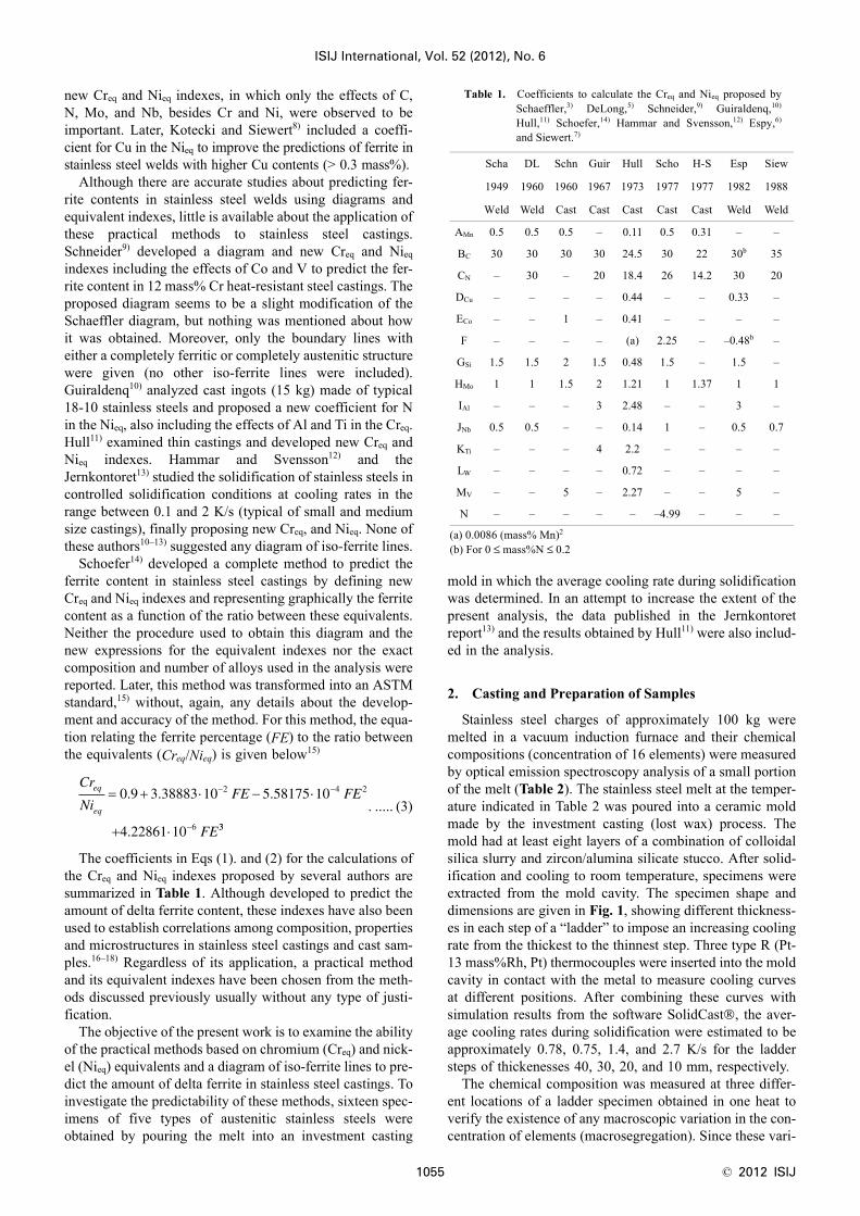
Stainless steel charges of approximately 100 kg weremelted in a vacuum induction furnace and their chemicalcompositions (concentration of 16 elements) were measuredby optical emission spectroscopy analysis of a small portionof the melt (Table 2). The stainless steel melt at the temper-ature indicated in Table 2 was poured into a ceramic moldmade by the investment casting (lost wax) process. Themold had at least eight layers of a combination of colloidalsilica slurry and zircon/alumina silicate stucco. After solid-ification and cooling to room temperature, specimens wereextracted from the mold cavity. The specimen shape anddimensions are given in Fig. 1, showing different thickness-es in each step of a “ladder” to impose an increasing coolingrate from the thickest to the thinnest step. Three type R (Pt-13 mass%Rh, Pt) thermocouples were inserted into the moldcavity in contact with the metal to measure cooling curvesat different positions. After combining these curves withsimulation results from the software SolidCast®, the aver-age cooling rates during solidification were estimated to beapproximately 0.78, 0.75, 1.4, and 2.7 K/s for the laddersteps of thickenesses 40, 30, 20, and 10 mm, respectively.

The chemical composition was measured at three differ-ent locations of a ladder specimen obtained in one heat toverify the existence of any macroscopic variation in the con-centration of elements (macrosegregation). Since these vari-

Cr

NiFE FE

FE

eq

eq

= + ⋅ − ⋅

+ ⋅

− −

−

0 9 3 38883 10 5 58175 10

4 22861 10

2 4 2

6

. . .

. 33

Table 1. Coefficients to calculate the Creq and Nieq proposed bySchaeffler,3) DeLong,5) Schneider,9) Guiraldenq,10)

Hull,11) Schoefer,14) Hammar and Svensson,12) Espy,6)

and Siewert.7)

Scha DL Schn Guir Hull Scho H-S Esp Siew

1949 1960 1960 1967 1973 1977 1977 1982 1988

Weld Weld Cast Cast Cast Cast Cast Weld Weld

AMn 0.5 0.5 0.5 – 0.11 0.5 0.31 – –

BC 30 30 30 30 24.5 30 22 30b 35

CN – 30 – 20 18.4 26 14.2 30 20

DCu – – – – 0.44 – – 0.33 –

ECo – – 1 – 0.41 – – – –

F – – – – (a) 2.25 – –0.48b –

GSi 1.5 1.5 2 1.5 0.48 1.5 – 1.5 –

HMo 1 1 1.5 2 1.21 1 1.37 1 1

IAl – – – 3 2.48 – – 3 –

JNb 0.5 0.5 – – 0.14 1 – 0.5 0.7

KTi – – – 4 2.2 – – – –

LW – – – – 0.72 – – – –

MV – – 5 – 2.27 – – 5 –

N – – – – – –4.99 – – –

(a) 0.0086 (mass% Mn)2

(b) For 0 ≤ mass%N ≤ 0.2

© 2012 ISIJ 1056

ISIJ International, Vol. 52 (2012), No. 6

ations were within the experimental error of the analyticaltechnique, macrosegregation of elements was not signifi-cant.

The delta ferrite content was determined with a Fischerferitscope model MP30E at several locations on a longitu-dinal section of the ladder specimens, yielding a completedelta ferrite distribution. The delta ferrite morphologieswere observed by optical metallography after preparation ofsamples by grinding, mechanical polishing with diamondpaste, and finally etching with aqua regia (100 ml HCl + 3 mlHNO3 + 100 ml methyl alcohol).

3. Measurements of Delta Ferrite Content

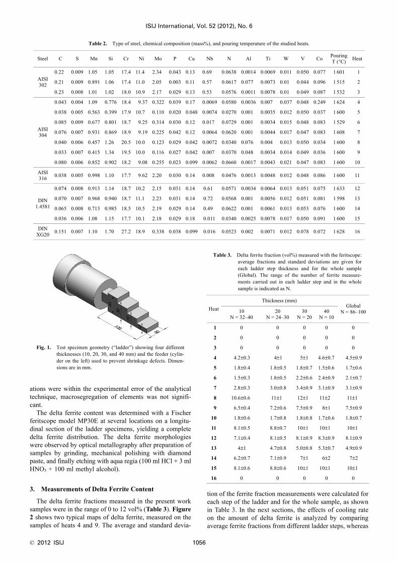
The delta ferrite fractions measured in the present worksamples were in the range of 0 to 12 vol% (Table 3). Figure2 shows two typical maps of delta ferrite, measured on thesamples of heats 4 and 9. The average and standard devia-

tion of the ferrite fraction measurements were calculated foreach step of the ladder and for the whole sample, as shownin Table 3. In the next sections, the effects of cooling rateon the amount of delta ferrite is analyzed by comparingaverage ferrite fractions from different ladder steps, whereas

Table 2. Type of steel, chemical composition (mass%), and pouring temperature of the studied heats.

Steel C S Mn Si Cr Ni Mo P Cu Nb N Al Ti W V Co PouringT (°C) Heat

AISI302

0.22 0.009 1.05 1.05 17.4 11.4 2.34 0.043 0.13 0.69 0.0638 0.0014 0.0069 0.011 0.050 0.077 1 601 1

0.21 0.009 0.891 1.06 17.4 11.0 2.05 0.003 0.11 0.57 0.0617 0.077 0.0073 0.01 0.044 0.096 1 515 2

0.23 0.008 1.01 1.02 18.0 10.9 2.17 0.029 0.13 0.53 0.0576 0.0011 0.0078 0.01 0.049 0.087 1 532 3

AISI304

0.043 0.004 1.09 0.776 18.4 9.37 0.322 0.039 0.17 0.0069 0.0580 0.0036 0.007 0.037 0.048 0.249 1 624 4

0.038 0.005 0.563 0.399 17.9 10.7 0.110 0.020 0.048 0.0074 0.0270 0.001 0.0035 0.012 0.050 0.037 1 600 5

0.085 0.009 0.677 0.801 18.7 9.25 0.314 0.030 0.12 0.017 0.0729 0.001 0.0034 0.015 0.048 0.083 1 529 6

0.076 0.007 0.931 0.869 18.9 9.19 0.225 0.042 0.12 0.0064 0.0620 0.001 0.0044 0.017 0.047 0.083 1 608 7

0.040 0.006 0.457 1.26 20.5 10.0 0.123 0.029 0.042 0.0072 0.0340 0.076 0.004 0.013 0.050 0.034 1 600 8

0.033 0.007 0.415 1.34 19.5 10.0 0.116 0.027 0.042 0.007 0.0370 0.048 0.0034 0.014 0.049 0.036 1 600 9

0.080 0.006 0.852 0.902 18.2 9.08 0.255 0.023 0.099 0.0062 0.0660 0.0017 0.0043 0.021 0.047 0.083 1 600 10

AISI316 0.038 0.005 0.998 1.10 17.7 9.62 2.20 0.030 0.14 0.008 0.0476 0.0013 0.0048 0.012 0.048 0.086 1 600 11

DIN1.4581

0.074 0.008 0.913 1.14 18.7 10.2 2.15 0.031 0.14 0.61 0.0571 0.0034 0.0064 0.013 0.051 0.075 1 633 12

0.070 0.007 0.968 0.940 18.7 11.1 2.23 0.031 0.14 0.72 0.0568 0.001 0.0056 0.012 0.051 0.081 1 598 13

0.065 0.008 0.713 0.985 18.5 10.5 2.19 0.029 0.14 0.49 0.0622 0.001 0.0061 0.013 0.053 0.076 1 600 14

0.036 0.006 1.08 1.15 17.7 10.1 2.18 0.029 0.18 0.011 0.0340 0.0025 0.0078 0.017 0.050 0.091 1 600 15

DINXG20 0.151 0.007 1.10 1.70 27.2 18.9 0.338 0.038 0.099 0.016 0.0523 0.002 0.0071 0.012 0.078 0.072 1 628 16

Fig. 1. Test specimen geometry (“ladder”) showing four differentthicknesses (10, 20, 30, and 40 mm) and the feeder (cylin-der on the left) used to prevent shrinkage defects. Dimen-sions are in mm.

Table 3. Delta ferrite fraction (vol%) measured with the feritscope:average fractions and standard deviations are given foreach ladder step thickness and for the whole sample(Global). The range of the number of ferrite measure-ments carried out in each ladder step and in the wholesample is indicated as N.

HeatThickness (mm)

GlobalN = 86–10010

N = 32–4020

N = 24–3030

N = 2040

N = 10

1 0 0 0 0 0

2 0 0 0 0 0

3 0 0 0 0 0

4 4.2±0.3 4±1 5±1 4.6±0.7 4.5±0.9

5 1.8±0.4 1.8±0.5 1.8±0.7 1.5±0.6 1.7±0.6

6 1.5±0.3 1.8±0.5 2.2±0.6 2.4±0.9 2.1±0.7

7 2.8±0.3 3.0±0.8 3.4±0.9 3.1±0.9 3.1±0.9

8 10.6±0.6 11±1 12±1 11±2 11±1

9 6.5±0.4 7.2±0.6 7.5±0.9 8±1 7.5±0.9

10 1.8±0.6 1.7±0.8 1.8±0.8 1.7±0.6 1.8±0.7

11 8.1±0.5 8.8±0.7 10±1 10±1 10±1

12 7.1±0.4 8.1±0.5 8.1±0.9 8.3±0.9 8.1±0.9

13 4±1 4.7±0.8 5.0±0.8 5.3±0.7 4.9±0.9

14 6.2±0.7 7.1±0.9 7±1 6±2 7±2

15 8.1±0.6 8.8±0.6 10±1 10±1 10±1

16 0 0 0 0 0

ISIJ International, Vol. 52 (2012), No. 6

1057 © 2012 ISIJ

the effects of composition is examined by comparing theglobal averages from different samples, i.e., different heats.

4. Effect of Cooling Rate on the Amount of Delta Fer-rite

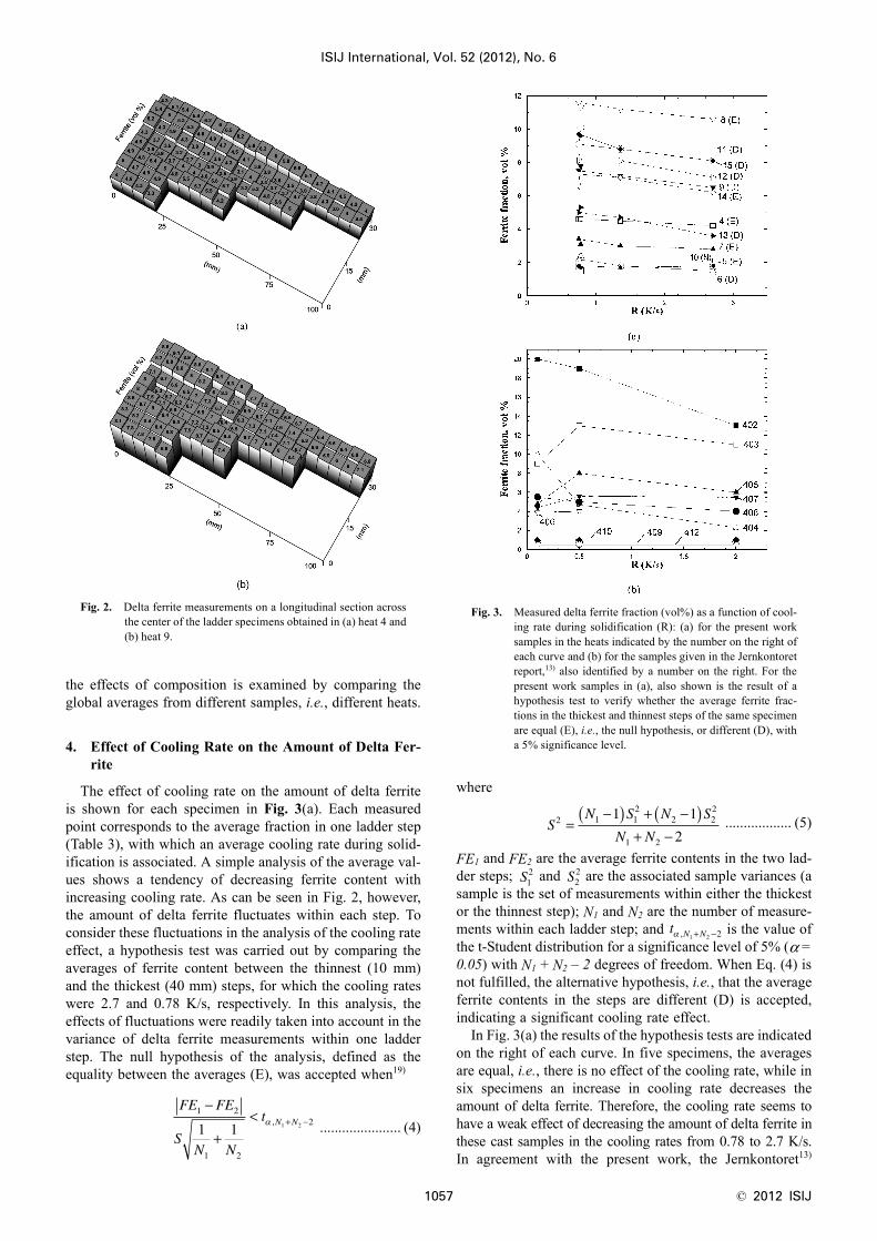
The effect of cooling rate on the amount of delta ferriteis shown for each specimen in Fig. 3(a). Each measuredpoint corresponds to the average fraction in one ladder step(Table 3), with which an average cooling rate during solid-ification is associated. A simple analysis of the average val-ues shows a tendency of decreasing ferrite content withincreasing cooling rate. As can be seen in Fig. 2, however,the amount of delta ferrite fluctuates within each step. Toconsider these fluctuations in the analysis of the cooling rateeffect, a hypothesis test was carried out by comparing theaverages of ferrite content between the thinnest (10 mm)and the thickest (40 mm) steps, for which the cooling rateswere 2.7 and 0.78 K/s, respectively. In this analysis, theeffects of fluctuations were readily taken into account in thevariance of delta ferrite measurements within one ladderstep. The null hypothesis of the analysis, defined as theequality between the averages (E), was accepted when19)

...................... (4)

where

.................. (5)

FE1 and FE2 are the average ferrite contents in the two lad-der steps; and are the associated sample variances (asample is the set of measurements within either the thickestor the thinnest step); N1 and N2 are the number of measure-ments within each ladder step; and is the value ofthe t-Student distribution for a significance level of 5% (α =0.05) with N1 + N2 – 2 degrees of freedom. When Eq. (4) isnot fulfilled, the alternative hypothesis, i.e., that the averageferrite contents in the steps are different (D) is accepted,indicating a significant cooling rate effect.

In Fig. 3(a) the results of the hypothesis tests are indicatedon the right of each curve. In five specimens, the averagesare equal, i.e., there is no effect of the cooling rate, while insix specimens an increase in cooling rate decreases theamount of delta ferrite. Therefore, the cooling rate seems tohave a weak effect of decreasing the amount of delta ferrite inthese cast samples in the cooling rates from 0.78 to 2.7 K/s.In agreement with the present work, the Jernkontoret13)

Fig. 2. Delta ferrite measurements on a longitudinal section acrossthe center of the ladder specimens obtained in (a) heat 4 and(b) heat 9.

FE FE

SN N

t N N1 2

1 2

21 1 1 2

−

+< + −α ,

Fig. 3. Measured delta ferrite fraction (vol%) as a function of cool-ing rate during solidification (R): (a) for the present worksamples in the heats indicated by the number on the right ofeach curve and (b) for the samples given in the Jernkontoretreport,13) also identified by a number on the right. For thepresent work samples in (a), also shown is the result of ahypothesis test to verify whether the average ferrite frac-tions in the thickest and thinnest steps of the same specimenare equal (E), i.e., the null hypothesis, or different (D), witha 5% significance level.

SN S N S

N N2 1 1

22 2

2

1 2

1 1

2=

−( ) + −( )+ −

S12 S2

2

t N Nα , 1 2 2+ −

© 2012 ISIJ 1058

ISIJ International, Vol. 52 (2012), No. 6

showed a negligible effect of the cooling rate during solid-ification (in the range between 0.1 and 2 K/s) on the amountof delta ferrite measured just below the solidus temperature.On cooling to room temperature, the ferrite content changedto a final fraction presented in Fig. 3(b). The authors13) didnot discuss the effects of cooling rate on this delta ferritefraction (measured after cooling to room temperature), butthe results given in Fig. 3(b) do not show any clear tenden-cy, confirming the weak effect of the cooling rate.

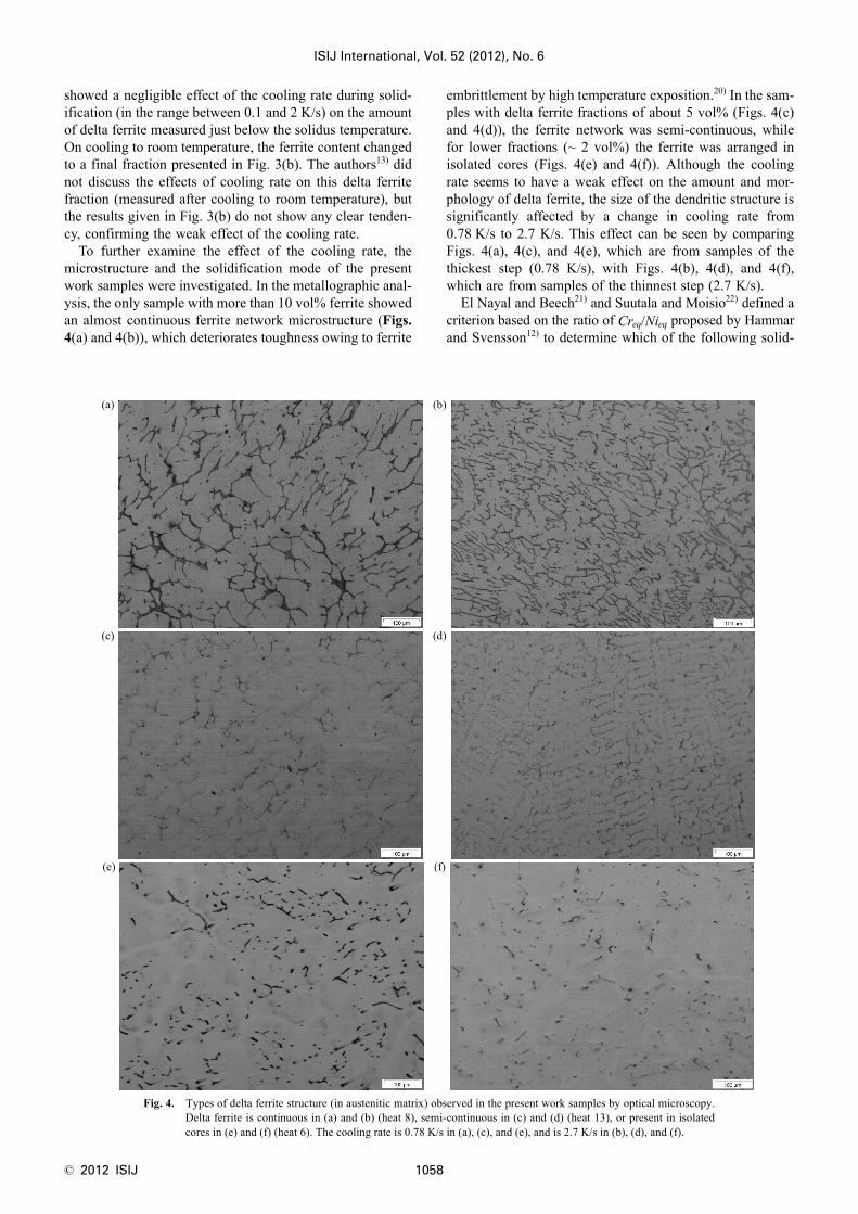
To further examine the effect of the cooling rate, themicrostructure and the solidification mode of the presentwork samples were investigated. In the metallographic anal-ysis, the only sample with more than 10 vol% ferrite showedan almost continuous ferrite network microstructure (Figs.4(a) and 4(b)), which deteriorates toughness owing to ferrite

embrittlement by high temperature exposition.20) In the sam-ples with delta ferrite fractions of about 5 vol% (Figs. 4(c)and 4(d)), the ferrite network was semi-continuous, whilefor lower fractions (~ 2 vol%) the ferrite was arranged inisolated cores (Figs. 4(e) and 4(f)). Although the coolingrate seems to have a weak effect on the amount and mor-phology of delta ferrite, the size of the dendritic structure issignificantly affected by a change in cooling rate from0.78 K/s to 2.7 K/s. This effect can be seen by comparingFigs. 4(a), 4(c), and 4(e), which are from samples of thethickest step (0.78 K/s), with Figs. 4(b), 4(d), and 4(f),which are from samples of the thinnest step (2.7 K/s).

El Nayal and Beech21) and Suutala and Moisio22) defined acriterion based on the ratio of Creq/Nieq proposed by Hammarand Svensson12) to determine which of the following solid-

(a) (b)

(c) (d)

(e) (f)

Fig. 4. Types of delta ferrite structure (in austenitic matrix) observed in the present work samples by optical microscopy.Delta ferrite is continuous in (a) and (b) (heat 8), semi-continuous in (c) and (d) (heat 13), or present in isolatedcores in (e) and (f) (heat 6). The cooling rate is 0.78 K/s in (a), (c), and (e), and is 2.7 K/s in (b), (d), and (f).

ISIJ International, Vol. 52 (2012), No. 6

1059 © 2012 ISIJ

ification modes is observed in austenitic stainless steels:mode A (L→L + γ→γ), mode AF (L→L + γ→ L + γ + δ→γ + δ), or mode FA (L→L + δ → L + δ + γ→γ + δ). Inthis sequence, L is the liquid phase, γ is austenite and δ isferrite. According to this criterion, heats 1, 2, 3, and 16solidified in mode A; therefore, the related microstructuresdid not have any ferrite. On the other hand, samples fromheats 4 to 15, which showed some delta ferrite in the micro-structure, solidified in mode FA, i.e., with ferrite as the lead-ing phase and formation of interdendritic austenite at theexpense of ferrite dendrites during solidification. Aftersolidification, during cooling to room temperature, furtheraustenite might form, consuming ferrite. In the FA mode,the change from ferrite to austenite depends on the diffusionof solute elements in the solid phases.

For samples solidifying in mode FA, Pereira and Beech23)

showed that no ferrite would be present at room temperatureif equilibrium conditions prevailed. Consequently, the exis-tence of ferrite at room temperature is an indication of lim-ited solute diffusion caused by relatively large cooling rates.An increase in cooling rate both during and after solidifica-tion (on cooling to room temperature) should increase theamount of ferrite at room temperature, as observed byElmer24) and Pereira and Beech.23) Nevertheless, Pereira andBeech,23) and Kim et al.25) observed that, in relatively largeingots and plates, in which the cooling rates change signif-icantly along the ingot cross section, there is a decrease inferrite content towards the ingot surface, where the largestcooling rate exists. Kim et al.25) investigated this behaviorin detail and showed that the importance of diffusion in pro-moting the δ →γ transformation actually depends on both

and λ, where D is the solute diffusion coefficient inthe solid, t is the time available for diffusion (during andafter solidification), and λ is the spacing between secondarydendrite arms. Brody and Flemings,26) and Flemings27)

showed that solid diffusion is more pronounced for larger values, where Fo is the mass diffusion

Fourier number. As briefly explained in the Jernkontoret13)

report, the faster cooling rate at the ingot surface, comparedwith its center, produces a fine dendritic structure that canbe more rapidly homogenized on cooling below the solidus.This more important role of diffusion at the surface ratherthan at the center of ingots has also been verified in studiesof microsegregation.28)

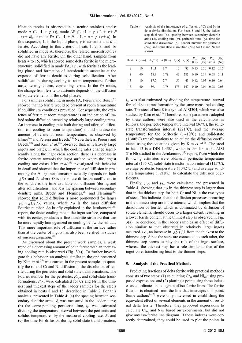
As discussed about the present work samples, a weaktrend of a decreasing amount of delta ferrite with an increas-ing cooling rate is observed (Fig. 3(a)). To further investi-gate this behavior, an analysis similar to the one presentedby Kim et al.25) was carried in the present samples to quan-tify the role of Cr and Ni diffusion in the dissolution of fer-rite during the peritectic and solid state transformations. TheFourier number for the peritectic, Fop, and solid-state trans-formations, Fos, were calculated for Cr and Ni in the thin-nest and thickest steps of the ladder samples for the steelsobtained in heats 8 and 13, described in Table 2. For thisanalysis, presented in Table 4: (a) the spacing between sec-ondary dendrite arms, λ, was measured in the ladder steps;(b) the corresponding peritectic time, tp, was estimateddividing the temperature interval between the peritectic andsolidus temperatures by the measured cooling rate, R; and(c) the time for diffusion during solid-state transformation,

ts, was also estimated by dividing the temperature intervalfor solid-state transformation by the same measured coolingrate. The steel of heat 8 is a typical AISI304, which was alsostudied by Kim et al.25) Therefore, some parameters adoptedby these authors were also used in the calculations asfollows: the peritectic temperature interval (36°C), the solid-state transformation interval (221°C), and the averagetemperature for the peritectic (1 410°C) and solid-state(1 300°C) transformations to calculate the diffusion coeffi-cients using the equations given by Kim et al.25) The steelin heat 13 is a DIN 1.4581, which is similar to the AISI316 Nb studied in the Jernkontoret13) report, from which thefollowing estimates were obtained: peritectic temperatureinterval (135°C), solid-state transformation interval (115°C),average peritectic temperature (1 342°C) and average solid-state temperature (1 218°C) to calculate the diffusion coef-ficients.

Finally, Fop and Fos were calculated and presented inTable 4, showing that Fo in the thinnest step is larger thanthat in the thickest step for both Cr and Ni in the two typesof steel. This indicates that the diffusion processes occurringin the thinnest step are more intense, which implies that thedissolution of ferrite, which is dominated by diffusion ofsolute elements, should occur to a larger extent, resulting ina lower ferrite content at the thinnest step as observed in Fig.3(a). To conclude, in the ladder samples an effect of diffu-sion similar to that observed in relatively large ingotsoccurred, i.e., an increase in from the thickest to thethinnest step. Since the steps are connected to each other, thethinnest step seems to play the role of the ingot surface,whereas the thickest step has a role similar to that of theingot core, transferring heat to the thinner steps.

5. Analysis of the Practical Methods

Predicting fractions of delta ferrite with practical methodsconsists of two steps: (1) calculating Creq and Nieq using pro-posed expressions and (2) plotting a point using these index-es as coordinates in a diagram of iso-ferrite lines. The ferritefraction is obtained from the line that intercepts this point.Some authors9–12) were only interested in establishing theequivalent effect of several elements in the amount of resid-ual delta ferrite. Therefore, they proposed expressions tocalculate Creq and Nieq based on experiments, but did notgive any iso-ferrite line diagram. If these indexes were cor-rectly determined, they could be used to plot the points in

Dt

Fo D t= / λ

Table 4. Analysis of the importance of diffusion of Cr and Ni indelta ferrite dissolution. For heats 8 and 13, the ladderstep thickness (L), spacing between secondary dendritearms (λ), cooling rate (R), peritectic time (tp), time forsolid-state dissolution (ts), Fourier number for peritectic(Fop) and solid state dissolution (Fos) for Cr and Ni areshown.

Heat L (mm) λ (μm) R (K/s) tp (s) ts (s) Fop(Cr)

Fos(Cr)

Fop(Ni)

Fos(Ni)

8 10 11.1 2.7 13 82 0.15 0.20 0.12 0.16

8 40 28.9 0.78 46 283 0.10 0.14 0.08 0.11

13 10 17.7 2.7 50 43 0.12 0.05 0.10 0.04

13 40 39.4 0.78 173 147 0.10 0.04 0.08 0.03

Dt / λ

© 2012 ISIJ 1060

ISIJ International, Vol. 52 (2012), No. 6

an iso-ferrite line diagram obtained by a different author,finally determining the ferrite fraction. Theoretically, theseiso-ferrite lines could be obtained using alloy compositionscompletely different from those used to obtain Creq and Nieq.For example, an iso-ferrite line diagram could be construct-ed using simple ternary Fe–Cr–Ni alloys and these linescould, in principle, be used in combination with the Creq andNieq expressions derived by Hull11) to estimated the ferritefraction. Consequently, combinations of Creq and Nieq index-es and iso-ferrite line diagrams proposed by differentauthors were adopted to predict the residual ferrite contentin the present work samples.

Nineteen versions of practical methods were defined bya combination of an expression to calculate Creq and Nieq

(step 1) and a diagram of iso-ferrite line (step 2). Each meth-od was analyzed by comparing its estimates with the exper-imental fractions obtained in the present work specimensand those given in the reports presented by theJernkontoret13) and by Hull.11) The ferrite fractions presentedby Hull11) were measured in pins (5.1 cm in length and0.6 cm in diameter) of 70 types of alloys cast in coppermolds. The fractions reported by the Jernkontoret13) wereobtained from samples cooled in a special furnace thatimposed cooling rates (0.1 to 2 K/s) typical of those in smalland medium size castings.

5.1. Equations Describing the Diagrams of Iso-ferriteLines

As described before, to predict delta ferrite fractions withpractical methods the values of Creq and Nieq calculated fora specific alloy composition should be used to plot a pointin a diagram of iso-ferrite lines. The line intercepting thispoint gives the amount of ferrite. If the point is located inbetween two iso-ferrite lines, some type of interpolation isnecessary. Therefore, the iso-ferrite lines of four importantdiagrams were represented by equations.

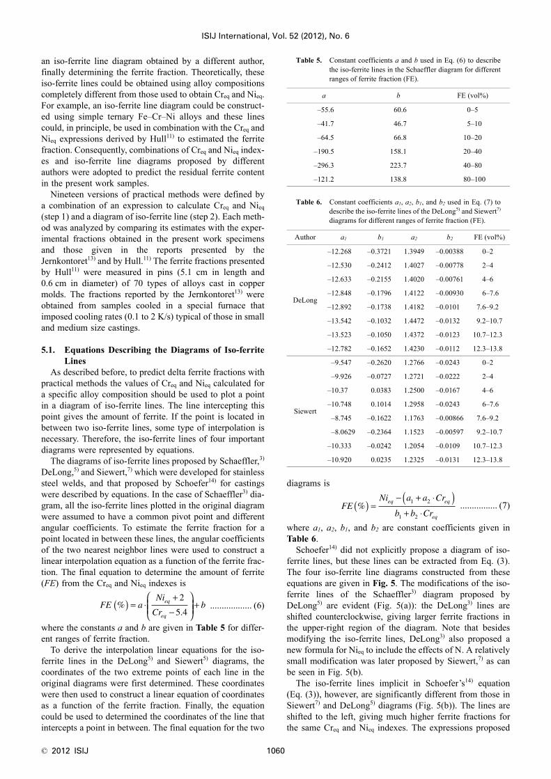
The diagrams of iso-ferrite lines proposed by Schaeffler,3)

DeLong,5) and Siewert,7) which were developed for stainlesssteel welds, and that proposed by Schoefer14) for castingswere described by equations. In the case of Schaeffler3) dia-gram, all the iso-ferrite lines plotted in the original diagramwere assumed to have a common pivot point and differentangular coefficients. To estimate the ferrite fraction for apoint located in between these lines, the angular coefficientsof the two nearest neighbor lines were used to construct alinear interpolation equation as a function of the ferrite frac-tion. The final equation to determine the amount of ferrite(FE) from the Creq and Nieq indexes is

.................. (6)

where the constants a and b are given in Table 5 for differ-ent ranges of ferrite fraction.

To derive the interpolation linear equations for the iso-ferrite lines in the DeLong5) and Siewert5) diagrams, thecoordinates of the two extreme points of each line in theoriginal diagrams were first determined. These coordinateswere then used to construct a linear equation of coordinatesas a function of the ferrite fraction. Finally, the equationcould be used to determined the coordinates of the line thatintercepts a point in between. The final equation for the two

diagrams is

................ (7)

where a1, a2, b1, and b2 are constant coefficients given inTable 6.

Schoefer14) did not explicitly propose a diagram of iso-ferrite lines, but these lines can be extracted from Eq. (3).The four iso-ferrite line diagrams constructed from theseequations are given in Fig. 5. The modifications of the iso-ferrite lines of the Schaeffler3) diagram proposed byDeLong5) are evident (Fig. 5(a)): the DeLong3) lines areshifted counterclockwise, giving larger ferrite fractions inthe upper-right region of the diagram. Note that besidesmodifying the iso-ferrite lines, DeLong3) also proposed anew formula for Nieq to include the effects of N. A relativelysmall modification was later proposed by Siewert,7) as canbe seen in Fig. 5(b).

The iso-ferrite lines implicit in Schoefer’s14) equation(Eq. (3)), however, are significantly different from those inSiewert7) and DeLong5) diagrams (Fig. 5(b)). The lines areshifted to the left, giving much higher ferrite fractions forthe same Creq and Nieq indexes. The expressions proposed

FE aNi

Crbeq

eq

%.

( ) = ⋅+

−

⎛

⎝⎜⎜

⎞

⎠⎟⎟ +

2

5 4

Table 5. Constant coefficients a and b used in Eq. (6) to describethe iso-ferrite lines in the Schaeffler diagram for differentranges of ferrite fraction (FE).

a b FE (vol%)

–55.6 60.6 0–5

–41.7 46.7 5–10

–64.5 66.8 10–20

–190.5 158.1 20–40

–296.3 223.7 40–80

–121.2 138.8 80–100

Table 6. Constant coefficients a1, a2, b1, and b2 used in Eq. (7) todescribe the iso-ferrite lines of the DeLong5) and Siewert7)

diagrams for different ranges of ferrite fraction (FE).

Author a1 b1 a2 b2 FE (vol%)

DeLong

–12.268 –0.3721 1.3949 –0.00388 0–2

–12.530 –0.2412 1.4027 –0.00778 2–4

–12.633 –0.2155 1.4020 –0.00761 4–6

–12.848 –0.1796 1.4122 –0.00930 6–7.6

–12.892 –0.1738 1.4182 –0.0101 7.6–9.2

–13.542 –0.1032 1.4472 –0.0132 9.2–10.7

–13.523 –0.1050 1.4372 –0.0123 10.7–12.3

–12.782 –0.1652 1.4230 –0.0112 12.3–13.8

Siewert

–9.547 –0.2620 1.2766 –0.0243 0–2

–9.926 –0.0727 1.2721 –0.0222 2–4

–10.37 0.0383 1.2500 –0.0167 4–6

–10.748 0.1014 1.2958 –0.0243 6–7.6

–8.745 –0.1622 1.1763 –0.00866 7.6–9.2

–8.0629 –0.2364 1.1523 –0.00597 9.2–10.7

–10.333 –0.0242 1.2054 –0.0109 10.7–12.3

–10.920 0.0235 1.2325 –0.0131 12.3–13.8

FENi a a Cr

b b Cr

eq eq

eq

%( ) =− + ⋅( )

+ ⋅1 2

1 2

ISIJ International, Vol. 52 (2012), No. 6

1061 © 2012 ISIJ

by Schoefer14) to calculate Creq and Nieq are also significant-ly different (see Table 1) from those proposed by the previ-ous authors. As a result, some part of these large differencescancel out and the estimates of ferrite fractions given bySchoefer14) are not substantially different from those of theprevious authors.

5.2. Predictions and Error AnalysisFerrite fractions calculated with practical methods are

compared with three different sets of experimental fractions:(1) measured in the present work, (2) reported by the Jernk-ontoret,13) and (3) reported by Hull.11) Nineteen differentversions of practical methods were defined by combiningseveral expressions for the Creq and Nieq indexes with dif-ferent diagrams of iso-ferrite lines, which finally give anestimate of the ferrite fraction for a certain alloy composi-tion. Schaeffler,3) DeLong,5) Siewert,7) and Schoefer14) allproposed both a diagram and expressions for the Creq andNieq. Therefore, these were chosen for the analysis. On theother hand, Schneider,9) Hull,11) Hammar and Svensson,12)

Espy,6) and Guiraldenq10) suggested expressions for Creq andNieq (see Eqs. (1) and (2) and Table 1), but did not proposeany new diagram of iso-ferrite lines. Consequently, to cal-

culate the ferrite fractions, their expressions were combinedwith the diagrams suggested by Schaeffler,3) DeLong,5) andSiewert.7) In all, nineteen (= 4 + 3 × 5) different versions ofthe practical method were used to calculate ferrite fractionsfor each alloy composition as follows: Creq and Nieq wereobtained using Eqs. (1), (2), and the coefficients in Table 1,and the ferrite fractions were finally calculated with Eqs.(3), (6), and (7), and the coefficients in Tables 5 and 6 foreach iso-ferrite line diagram. The number of alloys analyzedfor each of the nineteen versions of the practical methodvaried between 37 and 276.

As shown in Table 1, four of the Creq and Nieq indexesadopted to define a practical method were developed fromstudies in weld samples, but are applied to the cast samplesanalyzed in the present work. Generally, the larger coolingrates in weld samples could result in different ferriteamounts from those in the present cast samples. However,the results presented in section and those published in theliterature have usually shown a weak effect of cooling rateon the amount of residual ferrite. In the samples reported bythe Jernkontoret13) (Fig. 3), for example, no clear trend isobserved in the cooling rate range between 0.1 and 2 K/s.Pereira and Beech23) observed variations of ferrite fractionsfrom approximately 5 to 8 vol% after increasing the coolingrate from 0.42 to 32 K/s for steels in solidification mode FA.Kim et al.25) noticed a change in the fraction of ferrite from4 to 8 vol% along the cross section of a plate. Therefore,owing to the relatively weak effect of cooling rate, indexesand iso-ferrite lines carefully developed from weld sampleswere also used to define some of the practical methods usedin the present work to predict ferrite quantity in cast sam-ples.

In the comparisons between calculated and measured fer-rite fractions, two groups of alloys were created: one groupwith composition in the restricted range given in Table 7and another group in the extended range. The restrictedrange defines a group that approximately fulfills all compo-sition ranges of the alloys employed to derive the Creq andNieq expressions and diagrams used in the present analysis.The extended range, on the other hand, obviously yielded alarger group of alloys and was defined to show the behaviorof the practical methods outside of the composition range inwhich they were developed. Basically, most of the measure-ments presented by Hull11) were not included in the restrict-ed range group, because the alloys belong to a much broaderrange of compositions. All the alloys with measured ferritefractions larger than 13.8 vol% were removed from thestudy, because this is the limit in DeLong5) diagram. In eachcalculation, when the values of Creq and Nieq for a givenalloy composition were out of the range for the diagram ofiso-ferrite lines, the corresponding alloy was also removedfrom the analysis.

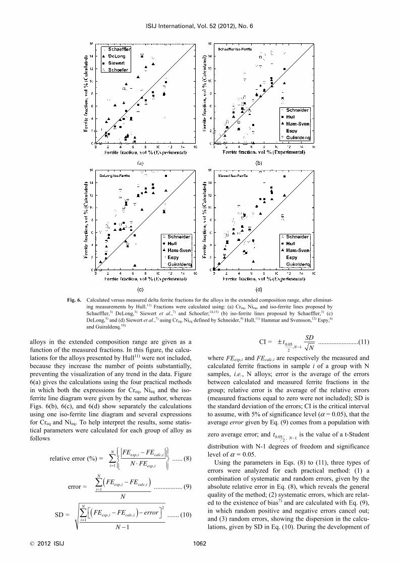
In Fig. 6, calculations of delta ferrite fractions using thenineteen versions of the practical methods applied to the

Fig. 5. Diagrams of iso-ferrite lines constructed from the equationsgiven in the present work: (a) Schaeffler3) and DeLong;5)

(b) Siewert,7) Schoefer,14) and DeLong.5)

Table 7. Restricted and extended composition ranges of element concentrations (mass%) used to define two groups of alloys.

C Mn Si Cr Ni Mo Cu Nb N Al Ti W V Co

Rest < 0.1 < 1.85 < 1.3 16–24 9–14 < 3 < 0.25 < 0.8 < 0.1 < 0.08 < 0.008 < 0.04 < 0.08 < 0.1

Ext < 0.3 < 20 < 4 12–32 4–25 < 6 < 4 < 4 < 0.2 < 2 < 2 < 5 < 4 < 6

© 2012 ISIJ 1062

ISIJ International, Vol. 52 (2012), No. 6

alloys in the extended composition range are given as afunction of the measured fractions. In this figure, the calcu-lations for the alloys presented by Hull11) were not included,because they increase the number of points substantially,preventing the visualization of any trend in the data. Figure6(a) gives the calculations using the four practical methodsin which both the expressions for Creq, Nieq and the iso-ferrite line diagram were given by the same author, whereasFigs. 6(b), 6(c), and 6(d) show separately the calculationsusing one iso-ferrite line diagram and several expressionsfor Creq and Nieq. To help interpret the results, some statis-tical parameters were calculated for each group of alloy asfollows

relative error (%) = ...... (8)

error = ................. (9)

SD = ....... (10)

CI = ........................(11)

where FEexp,i and FEcalc,i are respectively the measured andcalculated ferrite fractions in sample i of a group with Nsamples, i.e., N alloys; error is the average of the errorsbetween calculated and measured ferrite fractions in thegroup; relative error is the average of the relative errors(measured fractions equal to zero were not included); SD isthe standard deviation of the errors; CI is the critical intervalto assume, with 5% of significance level (α = 0.05), that theaverage error given by Eq. (9) comes from a population with

zero average error; and is the value of a t-Student

distribution with N-1 degrees of freedom and significancelevel of α = 0.05.

Using the parameters in Eqs. (8) to (11), three types oferrors were analyzed for each practical method: (1) acombination of systematic and random errors, given by theabsolute relative error in Eq. (8), which reveals the generalquality of the method; (2) systematic errors, which are relat-ed to the existence of bias7) and are calculated with Eq. (9),in which random positive and negative errors cancel out;and (3) random errors, showing the dispersion in the calcu-lations, given by SD in Eq. (10). During the development of

FE FE

N FE

i calc i

ii

Nexp

exp

, ,

,

−

⋅

⎧⎨⎪

⎩⎪

⎫⎬⎪

⎭⎪=∑

1

FE FE

N

i calc ii

N

exp, ,−( )=∑

1

FE FE error

N

i calc ii

N

exp, ,−( ) −⎡⎣

⎤⎦

−=∑

2

1

1

±−

tSD

NN0 05

21

.,

tN0 05

2 1. , −

Fig. 6. Calculated versus measured delta ferrite fractions for the alloys in the extended composition range, after eliminat-ing measurements by Hull.11) Fractions were calculated using: (a) Creq, Nieq, and iso-ferrite lines proposed bySchaeffler,3) DeLong,5) Siewert et al.,7) and Schoefer;14,15) (b) iso-ferrite lines proposed by Schaeffler,3) (c)DeLong,5) and (d) Siewert et al.,7) using Creq, Nieq defined by Schneider,9) Hull,11) Hammar and Svensson,12) Espy,6)

and Guiraldenq.10)

ISIJ International, Vol. 52 (2012), No. 6

1063 © 2012 ISIJ

a practical method, it becomes biased if important variables(e.g., specific chemical elements, processing conditions)that have an effect always in the same direction (i.e., alwayseither increase or decrease the ferrite fractions) are neglect-ed. The method was considered biased when the averageerror (Eq. (9)) was outside of the critical interval given byCI (Eq. (11)). Larger SD values suggest that important vari-ables that have random effects on the ferrite fractions werenot considered during development of the practical method.Note that the average relative error (Eq. (8)) indicates thecombined effects of systematic and random errors and tendto be low when these errors are low.

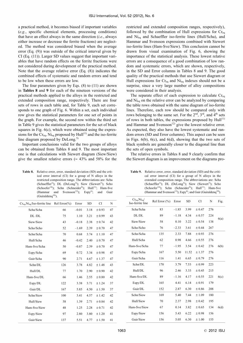
The four parameters given by Eqs. (8) to (11) are shownin Tables 8 and 9 for each of the nineteen versions of thepractical methods applied to the alloys in the restricted andextended composition range, respectively. There are foursets of rows in each table and, for Table 9, each set corre-sponds to one graph of Fig. 6. Within a set, each individualrow gives the statistical parameters for one set of points inthe graph. For example, the second row within the third setin Table 9 gives the statistical parameters for the set of blacksquares in Fig. 6(c), which were obtained using the expres-sions for the Creq, Nieq proposed by Hull11) and the iso-ferriteline diagram proposed by DeLong.5)

Important conclusions valid for the two groups of alloyscan be obtained from Tables 8 and 9. The most importantone is that calculations with Siewert diagram (Siew/Siew)give the smallest relative errors (≈ 43% and 58% for the

restricted and extended composition ranges, respectively),followed by the combination of Hull expressions for Creq

and Nieq and Schaeffler iso-ferrite lines (Hull/Scha), andHammar and Svensson expressions combined with Siewertiso-ferrite lines (Ham-Sve/Siew). This conclusion cannot bedrawn from visual examination of Fig. 6, showing theimportance of the statistical analysis. These lowest relativeerrors are a consequence of a good combination of low ran-dom and systematic errors, which are shown, respectively,in the SD and Error columns in Tables 8 and 9. The goodquality of the practical methods that use Siewert diagram orHull expressions for Creq and Nieq indexes should not be asurprise, since a very large number of alloy compositionswere considered in their analysis.

The separate effect of each expression to calculate Creq

and Nieq on the relative error can be analyzed by comparingthe table rows obtained with the same diagram of iso-ferritelines. Therefore, each row should be compared only withrows belonging to the same set. For the 2nd, 3rd, and 4th setsof rows in both tables, the expressions proposed by Hull11)

and Hammar and Svensson12) give the lowest relative error.As expected, they also have the lowest systematic and ran-dom errors (SD and Error columns). This aspect can be seenin Figs. 6(b), 6(c), and 6(d), showing that the two sets ofblack symbols are generally closer to the diagonal line thanthe sets of open symbols.

The relative errors in Tables 8 and 9 clearly confirm thatthe Siewert diagram is an improvement on the diagrams pro-

Table 8. Relative error, error, standard deviation (SD) and the crit-ical error interval (CI) for a group of N alloys in therestricted composition range. The abbreviations are: Scha(Schaeffler3)); DL (DeLong5)); Siew (Siewert7)); Scho(Schoefer14)); Schn (Schneider9)); Hull11); Ham-Sve(Hammar and Svensson12)); Espy6); and Guir(Guiraldenq10)).

Creq,Nieq/Iso-ferrite line Rel Error(%) Error SD CI N

Scha/Scha 66 –0.01 3.18 ± 0.93 47

DL /DL 75 1.10 3.21 ± 0.99 43

Siew/Siew 43 –0.18 2.38 ± 0.74 42

Scho/Scho 52 –1.69 2.39 ± 0.70 47

Schn/Scha 70 0.68 3.74 ± 1.10 47

Hull/Scha 46 –0.42 2.40 ± 0.70 47

Ham-Sve/Scha 50 –0.87 2.39 ± 0.70 47

Espy/Scha 69 0.72 3.34 ± 0.98 47

Guir/Scha 90 2.71 4.67 ± 1.37 47

Schn/DL 126 3.78 4.82 ± 1.48 43

Hull/DL 77 1.70 2.90 ± 0.90 42

Ham-Sve/DL 66 1.46 2.55 ± 0.80 42

Espy/DL 122 3.38 3.71 ± 1.24 37

Guir/DL 167 5.85 4.50 ± 1.50 37

Schn/Siew 100 3.41 4.57 ± 1.42 42

Hull/Siew 58 1.39 2.71 ± 0.84 42

Ham-Sve/Siew 48 1.25 2.28 ± 0.71 42

Espy/Siew 97 2.80 3.80 ± 1.20 41

Guir/Siew 137 5.51 4.77 ± 1.50 41

Table 9. Relative error, error, standard deviation (SD) and the criti-cal error interval (CI) for a group of N alloys in theextended composition range. The abbreviations are: Scha(Schaeffler3)); DL (DeLong5)); Siew (Siewert7)); Scho(Schoefer14)); Schn (Schneider9)); Hull11); Ham-Sve(Hammar and Svensson12)); Espy6); and Guir (Guiraldenq10)).

Creq,Nieq/Iso-ferrite line Rel Error (%) Error SD CI N Fig.

Scha/Scha 83 –1.85 3.99 ± 0.47 276

6(a)DL/DL 89 –1.18 4.34 ± 0.57 224

Siew/Siew 58 0.10 3.22 ± 0.54 138

Scho/Scho 76 –2.33 3.61 ± 0.44 267

Schn/Scha 135 2.33 7.88 ± 0.93 276

6(b)

Hull/Scha 62 0.98 4.66 ± 0.55 276

Ham-Sve/Scha 77 –1.95 3.54 ± 0.42 276

Espy/Scha 167 5.50 11.52 ± 1.37 276

Guir/Scha 116 1.41 6.65 ± 0.79 276

Schn/DL 170 3.79 7.53 ± 0.99 223

6(c)

Hull/DL 96 2.46 3.33 ± 0.45 215

Ham-Sve/DL 89 –1.16 4.17 ± 0.55 221

Espy/DL 165 4.41 6.14 ± 0.91 179

Guir/DL 152 2.87 6.30 ± 0.86 208

Schn/Siew 169 5.40 7.44 ± 1.09 180

6(d)

Hull/Siew 70 2.37 2.98 ± 0.42 195

Ham-Sve/Siew 67 0.14 3.82 ± 0.65 134

Espy/Siew 156 5.43 6.22 ± 0.98 156

Guir/Siew 156 5.05 6.30 ± 1.00 155

© 2012 ISIJ 1064

ISIJ International, Vol. 52 (2012), No. 6

posed by Schaeffler3) and DeLong,5) as intended by itsauthor. This can also be seen in Fig. 6(a), in which calcula-tions for the Schaeffler and DeLong diagrams are fartherfrom the diagonal line. These larger errors for the Schaefflerdiagram cannot be attributed to the differences in coolingrates between weld samples (used to construct Schaefflerdiagram) and the cast samples used in the present analysis,since the Siewert diagram was also developed for welds.Although Siewert diagram was constructed for weld sam-ples, its calculations for the cast samples examined in thepresent work gave errors lower than those methods speciallydeveloped for castings, i.e., Schoefer’s method14) and com-binations of Creq and Nieq given by Schneider9) andGuiraldenq.10) This suggests that the difference betweencooling rates experienced by weld and cast samples may notsignificantly change the amount of residual ferrite observedat room temperature, which agrees with the results presentedin Section 4 for the weak effect of cooling rate.

On the other hand, a simple examination of Figs. 6(c) and6(d) could give the impression that a clear trend exists of adecrease in the ferrite fraction with a decrease in the coolingrate. In these figures, most of the experimentally measuredfractions (for castings) are lower than the calculated frac-tions, obtained from iso-ferrite lines developed for weldsamples, in which the cooling rates are much higher. Nev-ertheless, Fig. 6(a) shows an opposite trend, i.e., measuredfractions are higher than most of the fractions calculatedwith Siewert diagram and higher than approximately half ofthe fractions calculated with DeLong diagrams. Both thesediagrams were developed from weld samples, in which thecooling rate is higher than that in cast samples, indicatingan increase in ferrite fraction with a decrease in cooling rate.The opposite trend observed in these figures might also sug-gest a weak effect of the cooling rate, easily outweighed byother effects and preventing a clear tendency from beingrevealed.

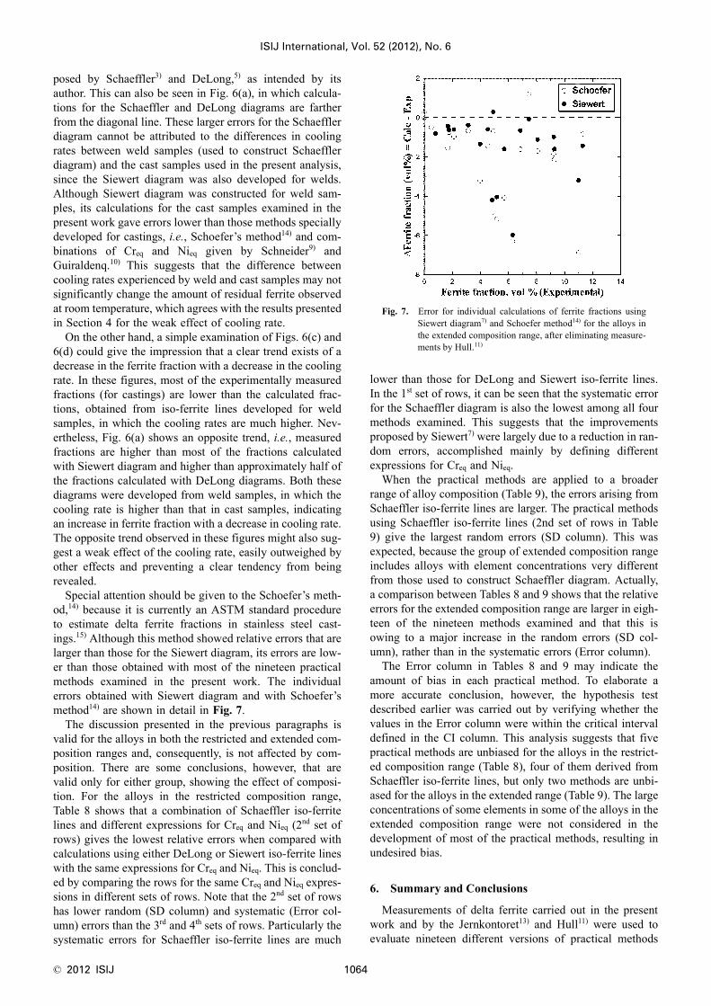
Special attention should be given to the Schoefer’s meth-od,14) because it is currently an ASTM standard procedureto estimate delta ferrite fractions in stainless steel cast-ings.15) Although this method showed relative errors that arelarger than those for the Siewert diagram, its errors are low-er than those obtained with most of the nineteen practicalmethods examined in the present work. The individualerrors obtained with Siewert diagram and with Schoefer’smethod14) are shown in detail in Fig. 7.

The discussion presented in the previous paragraphs isvalid for the alloys in both the restricted and extended com-position ranges and, consequently, is not affected by com-position. There are some conclusions, however, that arevalid only for either group, showing the effect of composi-tion. For the alloys in the restricted composition range,Table 8 shows that a combination of Schaeffler iso-ferritelines and different expressions for Creq and Nieq (2nd set ofrows) gives the lowest relative errors when compared withcalculations using either DeLong or Siewert iso-ferrite lineswith the same expressions for Creq and Nieq. This is conclud-ed by comparing the rows for the same Creq and Nieq expres-sions in different sets of rows. Note that the 2nd set of rowshas lower random (SD column) and systematic (Error col-umn) errors than the 3rd and 4th sets of rows. Particularly thesystematic errors for Schaeffler iso-ferrite lines are much

lower than those for DeLong and Siewert iso-ferrite lines.In the 1st set of rows, it can be seen that the systematic errorfor the Schaeffler diagram is also the lowest among all fourmethods examined. This suggests that the improvementsproposed by Siewert7) were largely due to a reduction in ran-dom errors, accomplished mainly by defining differentexpressions for Creq and Nieq.

When the practical methods are applied to a broaderrange of alloy composition (Table 9), the errors arising fromSchaeffler iso-ferrite lines are larger. The practical methodsusing Schaeffler iso-ferrite lines (2nd set of rows in Table9) give the largest random errors (SD column). This wasexpected, because the group of extended composition rangeincludes alloys with element concentrations very differentfrom those used to construct Schaeffler diagram. Actually,a comparison between Tables 8 and 9 shows that the relativeerrors for the extended composition range are larger in eigh-teen of the nineteen methods examined and that this isowing to a major increase in the random errors (SD col-umn), rather than in the systematic errors (Error column).

The Error column in Tables 8 and 9 may indicate theamount of bias in each practical method. To elaborate amore accurate conclusion, however, the hypothesis testdescribed earlier was carried out by verifying whether thevalues in the Error column were within the critical intervaldefined in the CI column. This analysis suggests that fivepractical methods are unbiased for the alloys in the restrict-ed composition range (Table 8), four of them derived fromSchaeffler iso-ferrite lines, but only two methods are unbi-ased for the alloys in the extended range (Table 9). The largeconcentrations of some elements in some of the alloys in theextended composition range were not considered in thedevelopment of most of the practical methods, resulting inundesired bias.

6. Summary and Conclusions

Measurements of delta ferrite carried out in the presentwork and by the Jernkontoret13) and Hull11) were used toevaluate nineteen different versions of practical methods

Fig. 7. Error for individual calculations of ferrite fractions usingSiewert diagram7) and Schoefer method14) for the alloys inthe extended composition range, after eliminating measure-ments by Hull.11)

ISIJ International, Vol. 52 (2012), No. 6

1065 © 2012 ISIJ

(nickel/chromium equivalent indexes and iso-ferrite linediagrams) to estimate residual ferrite fractions in austeniticstainless steel castings. Designed with different step thick-nesses, ladder shaped specimens cast in the present workshowed the effects of cooling rate on the amount of residualferrite in the microstructure.

In the ladder shaped samples, a change in cooling ratefrom 0.78 to 2.7 K/s has a weak effect on the amount of del-ta ferrite. In approximately 50% of the specimens with fer-rite in their microstructures, a hypothesis test indicates thatan increasing cooling rate decreases the amount of delta fer-rite, in agreement with some results presented by Kim etal.25) and Pereira and Beech.23) In the remaining specimens,no effect was detected. Optical microscopy showed that, forferrite fractions over 10 vol%, there is an almost continuousferrite network, whereas for ferrite fractions of about 5 vol%,the network becomes semi-continuous, changing to isolatedcores for fractions lower than approximately 2 vol%.

Calculations of ferrite fractions using the practical methodproposed by Siewert7) give the lowest relative error amongall the nineteen methods examined in the present work. Lowrelative errors were also obtained by two practical methodsusing the following combination: (a) nickel/chromiumequivalent indexes proposed by Hull11) with iso-ferrite linessuggested by Schaeffler3) and (b) nickel/chromium equiva-lent indexes proposed by Hammar and Svensson12) with iso-ferrite lines suggested by Siewert.7) These three practicalmethods give a good combination of low systematic andrandom errors. Although the Siewert diagram was construct-ed for stainless steel welds, estimates of ferrite fractionsusing this diagram in cast samples are more accurate thanthose calculated with the method of Schoefer,14) speciallydeveloped for cast samples and currently adopted as anASTM standard15) to predict residual ferrite fractions instainless steels castings.

When combined with any of the three diagrams of iso-ferrite lines proposed by Schaeffler,3) DeLong,5) or Siewert,7)

the expressions derived by Hull11) or by Hammar andSvensson12) to calculate the nickel and chromium equivalentindexes give the lowest relative error among all other equiv-alent index expressions. On the other hand, for alloys in arestricted composition range, expressions of nickel andchromium equivalents give the lowest relative errors whencombined with Schaeffler iso-ferrite lines. When alloys witha broader composition range are included in the analysis, the

relative errors increase in eighteen of the nineteen practicalmethods examined as a result of an increase in randomerrors.

AcknowledgementsThe authors wish to thank FAPESP (Fundação de

Amparo à Pesquisa do Estado de São Paulo) for the finan-cial support to this work (grants 95/9113-2, 96/04242-1, and03/08576-7) and Açotécnica SA for providing the samples.

REFERENCES

1) A. F. Padilha and P. R. Rios: ISIJ Int., 42 (2002), 325.2) D. L. Olson: Weld. J., 64 (1985), S281.3) A. L. Schaeffler: Met. Prog., 56 (1949), 680.4) S. Fukumoto, K. Fujiwara, S. Toji and A. Yamamoto: Mater. Sci.

Eng. A, 492 (2008), 243.5) W. T. DeLong: Met. Prog., 77 (1960), 98.6) R. H. Espy: Weld. J., 61 (1982), S149.7) T. A. Siewert, C. N. McCowan and D. L. Olson: Weld. J., 67 (1988),

S289.8) D. J. Kotecki and T. A. Siewert: Weld. J., 71 (1992), S171.9) H. Schneider: Foundry Trade J., 108 (1960), 562.

10) P. Guiraldenq: Mem. Sci. Rev. Met., 64 (1967), 907.11) F. C. Hull: Weld. J., 52 (1973), 193.12) Ö. Hammar and U. Svensson: Solidification and Casting of Metals,

The Metals Society, London, (1977), 401.13) Jernkontoret: A Guide to the Solidification of Steels, Jernkontoret,

Stockholm, (1977).14) E. A. Schoefer: Metal Progress Databook, 112 (1977), 51.15) ASTM Standard Practice for Steel Casting, Austenitic Alloy, Esti-

mating Ferrite Content Thereof (800/A 800M-01). Steel, StainlessSteel, and Related Alloys. ASTM International, West Conshohocken,Philadelphia, PA, (2006). 1.

16) Y.-H. Park and Z.-H. Lee: Mater. Sci. Eng. A, 297 (2001), 78.17) P. L. Ferrandini, C. T. Rios, A. T. Dutra, M. A. Jaime, P. R. Mei and

R. Caram: Mater. Sci. Eng. A, 435 (2006), 139.18) A. Di Schino, M. G. Mecozzi, M. Barteri and J. M. Kenny: J. Mater.

Sci., 35 (2000), 375.19) D. C. Montgomery and G. C. Runger: Applied Statistics and Proba-

bility for Engineers, Wiley, Hoboken, NJ, (2007).20) T. Yamada, S. Okano and H. Kuwano: J. Nucl. Mater., 350 (2006),

47.21) G. El Nayal and J. Beech: Mater. Sci. Technol., 2 (1986), 603.22) N. Suutala and T. Moisio: Solidification Technology in the Foundry

and Cast House, The Metals Society, London, (1980), 310.23) O. J. Pereira and J. Beech: Solidification Technology in the Foundry

and Cast House, The Metals Society, London, (1980), 315.24) J. W. Elmer, S. M. Allen and T. W. Eagar: Recent Trends in Welding

Science and Technology - TWR ’89, ASM International, MaterialsPark, Ohio, (1989), 169.

25) S. K. Kim, Y. K. Shin and N. J. Kim: Ironmaking Steelmaking, 22(1995), 316.

26) H. D. Brody and M. C. Flemings: Trans. Met. Soc. AIME, 236 (1966),615.

27) M. C. Flemings: Solidification processing, McGraw-Hill, New York,(1974).

28) M. A. Martorano and J. D. T. Capocchi: Metall. Mater. Trans. A, 31(2000), 3137.