Embed Size (px)
Citation preview

PREDICTING CREDIT DEFAULT RISK VIA STATISTICAL MODEL ANDMACHINE LEARNING ALGORITHMS
by
Anand Mohan Choubey
A thesis submitted to the faculty ofThe University of North Carolina at Charlotte
in partial ful�llment of the requirementsfor the degree of Master of Science in
Economics
Charlotte
2018
Approved by:
Dr. Craig A. Depken, II
Dr. L. Ted Amato
Dr. Matthew R. Metzgar

ii
c©2018Anand Mohan Choubey
ALL RIGHTS RESERVED

iii
ABSTRACT
ANAND MOHAN CHOUBEY. Predicting credit default risk via statistical modeland machine learning algorithms. (Under the direction of
DR. CRAIG A. DEPKEN, II)
Financial institutions need to measure risks within their credit portfolios (home
loans, credit card, auto loans, etc.) for regulatory requirements and for internal risk
management. To meet these requirements �nancial institutions increasingly rely on
models and algorithms to predict losses resulting from customers' defaults. Hence,
developing su�ciently accurate and robust models is one of the major e�orts of quan-
titative risk management groups within these institutions.
The proposed research is one such e�ort to develop robust and e�cient models for
the credit default risk problem. Speci�cally, the research focuses on developing a lo-
gistic regression based model and machine-learning based non-parametric algorithms
to predict default risk for credit card accounts. We use data named "default of credit
card clients data set" sourced from the University of California, Irvine to pursue this
study.
The thesis provides a systematic step-by-step model development approach - start-
ing from building a benchmark model, continually improving the benchmark model
by tuning the hyper-parameters, recursively eliminating insigni�cant variables from
the predictor pool, and then evaluating model on various performance measures - to
arrive at the best estimation for the model to implement on the training data.
Finally, based on the research �ndings, we provide insight into opportunities, and
future research in using machine-learning based modeling approaches for addressing
credit default risk.

iv
TABLE OF CONTENTS
LIST OF TABLES v
LIST OF FIGURES vi
LIST OF ABBREVIATIONS 1
CHAPTER 1: INTRODUCTION 1
CHAPTER 2: MODEL FRAMEWORK AND THEORY 4
2.1. Model framework 5
2.2. Logistic regression 6
2.3. Decision Tree, Random Forest 7
2.4. Arti�cial Neural Network 10
2.5. Model Evaluation 11
CHAPTER 3: MODEL DEVELOPMENT DATA 16
3.1. Target variable 16
3.2. Predictor variables 17
3.3. Training and Testing data 25
3.4. Class imbalance 25
CHAPTER 4: MODEL ESTIMATIONS AND RESULTS 27
4.1. Logistic regression model 28
4.2. Decision Tree and Random forest models 33
4.3. Models' performance results 36
CHAPTER 5: SUMMARY AND FUTURE RESEARCH 38
REFERENCES 40

v
LIST OF TABLES
TABLE 3.1: Variables used for model development 17
TABLE 3.2: Default rate (sorted descending) for di�erent segments 19
TABLE 4.1: Models' performance results 36

vi
LIST OF FIGURES
FIGURE 2.1: Logistic sigmoid model vs Linear regression model 7
FIGURE 2.2: A simple Decision Tree on the credit default data 9
FIGURE 2.3: A simple Random Forest framework 10
FIGURE 2.4: A simple ANN framework to model binary response 11
FIGURE 2.5: A confusion matrix 14
FIGURE 2.6: ROC curve and AUC score 14
FIGURE 3.1: Figure showing counts for 'defaults' and 'non-defaults' 17
FIGURE 3.2: Box-plots showing age distribution of customers 18
FIGURE 3.3: Default rate distributions for Male and Female 20
FIGURE 3.4: Default rate distributions for 'Marriage' variable 21
FIGURE 3.5: Default rate distributions by education levels 22
FIGURE 3.6: Correlation between variables 23
FIGURE 3.7: Default amt of balance limit grouped by default 24
FIGURE 3.8: 'Age' grouped by 'default' (density plot) 25
FIGURE 4.1: Confusion Matrix for the benchmark model 29
FIGURE 4.2: ROC curve and AUC score for the benchmark model 29
FIGURE 4.3: Model parameter estimate on the reduced predictor pool 31
FIGURE 4.4: Confusion matrix for the �nal logistic regression model 32
FIGURE 4.5: ROC curve for the �nal logistic regression model 33
FIGURE 4.6: A Decision Tree model for the credit card default problem 34
FIGURE 4.7: ROC curves for various models 37
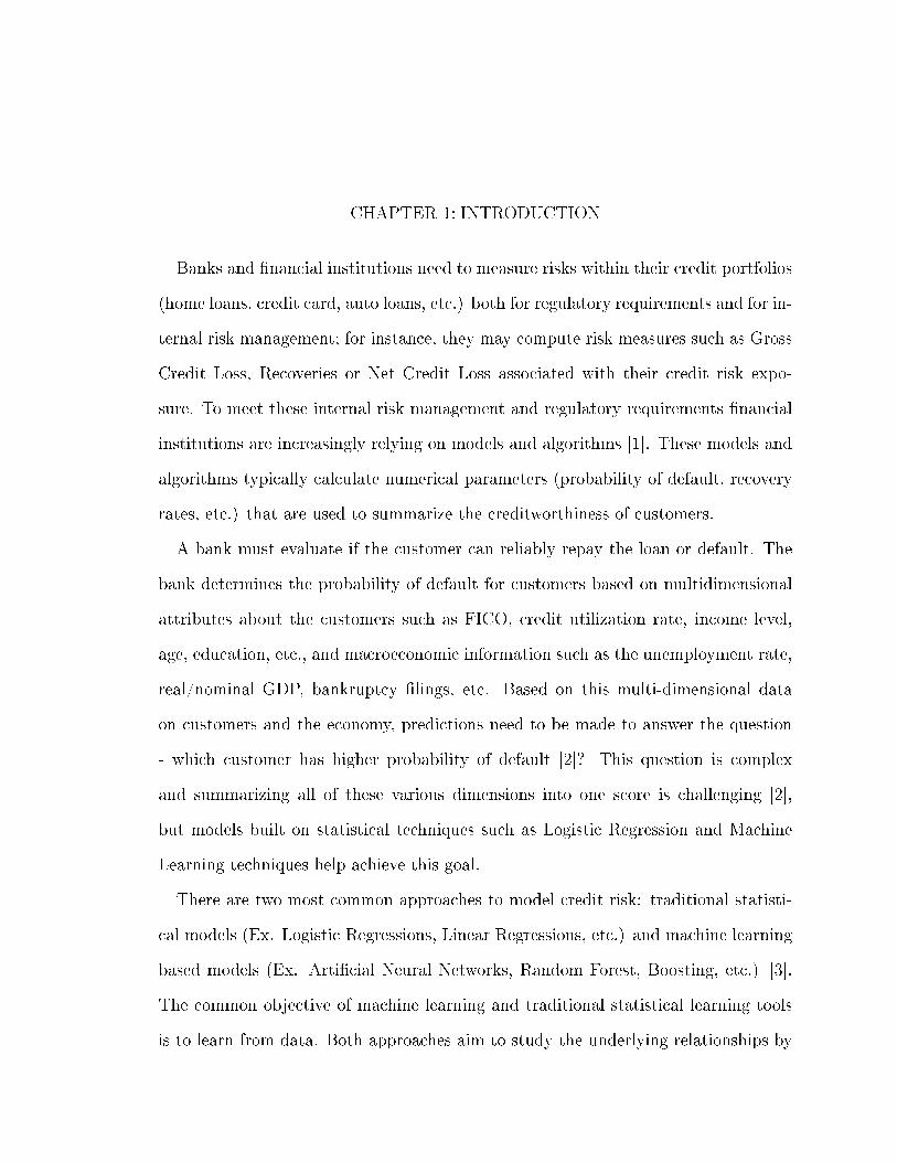
CHAPTER 1: INTRODUCTION
Banks and �nancial institutions need to measure risks within their credit portfolios
(home loans, credit card, auto loans, etc.) both for regulatory requirements and for in-
ternal risk management; for instance, they may compute risk measures such as Gross
Credit Loss, Recoveries or Net Credit Loss associated with their credit risk expo-
sure. To meet these internal risk management and regulatory requirements �nancial
institutions are increasingly relying on models and algorithms [1]. These models and
algorithms typically calculate numerical parameters (probability of default, recovery
rates, etc.) that are used to summarize the creditworthiness of customers.
A bank must evaluate if the customer can reliably repay the loan or default. The
bank determines the probability of default for customers based on multidimensional
attributes about the customers such as FICO, credit utilization rate, income level,
age, education, etc., and macroeconomic information such as the unemployment rate,
real/nominal GDP, bankruptcy �lings, etc. Based on this multi-dimensional data
on customers and the economy, predictions need to be made to answer the question
- which customer has higher probability of default [2]? This question is complex
and summarizing all of these various dimensions into one score is challenging [2],
but models built on statistical techniques such as Logistic Regression and Machine
Learning techniques help achieve this goal.
There are two most common approaches to model credit risk: traditional statisti-
cal models (Ex. Logistic Regressions, Linear Regressions, etc.) and machine learning
based models (Ex. Arti�cial Neural Networks, Random Forest, Boosting, etc.) [3].
The common objective of machine learning and traditional statistical learning tools
is to learn from data. Both approaches aim to study the underlying relationships by

2
using a training dataset. Typically, statistical learning methods assume formal re-
lationships between variables in the form of mathematical equations, while machine
learning (ML) methods can learn from data without requiring any rule-based pro-
gramming [2]. As a result of this �exibility, machine learning methods can better
�t the patterns in data and are better equipped to capture the non-linear relation-
ships common to credit risk modeling problems. However, at the same time, these
models run the risk of over-�tting, and the predictions made by ML approaches are
sometimes di�cult to explain due to their complex "black box" nature [2].
In this research, we construct nonlinear, parametric and non-parametric credit risk
models based on statistical and machine-learning techniques to predict default risk
for credit card accounts.
This thesis provides a systematic step-by-step model development approach to
statistical and machine learning models to model a practical credit risk problem to
predict customers who would potentially default - starting from building a benchmark
model, continually improving the benchmark model by tuning the hyper-parameter,
recursively eliminating insigni�cant variables from the predictor pool, and then eval-
uating model on various performance metrics that are relevant for this problem - to
�nally arrive at the best estimation for the model to implement on the training data.
The research applies the industry's most popular tool for such default probability
prediction problems - Logistic Regression, and also applies other newer nonpara-
metric, machine learning algorithms - Decision Trees, Random Forest, and ANN to
investigate their performance and applicability to the problem.
The rest of the thesis is organized as follows. Chapter 2 establishes the foundation
and model development framework for investigating the proposed research. It pro-
vides the theory on various models, model evaluation to establish the context for the
readers and foundation leading to the development of these models for the problem.
Chapter 3 provides an extensive exploratory data analyses to provide insight into

3
the data; the study also includes determining training and testing data sets and
balancing the training data based on response variable before using it in the model
estimation process.
Chapter 4 implements a systematic model estimation approach, implements statis-
tical and machine learning models on the credit card default problem and discusses
models' performance on key metrics.
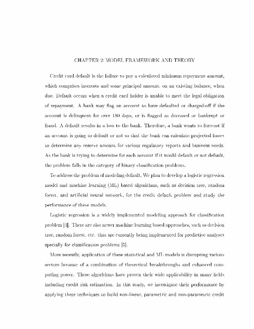
CHAPTER 2: MODEL FRAMEWORK AND THEORY
Credit card default is the failure to pay a calculated minimum repayment amount,
which comprises interests and some principal amount, on an existing balance, when
due. Default occurs when a credit card holder is unable to meet the legal obligation
of repayment. A bank may �ag an account to have defaulted or charged-o� if the
account is delinquent for over 180 days, or is �agged as deceased or bankrupt or
fraud. A default results in a loss to the bank. Therefore, a bank wants to forecast if
an account is going to default or not so that the bank can calculate projected losses
to determine any reserve amount for various regulatory reports and business needs.
As the bank is trying to determine for each account if it would default or not default,
the problem falls in the category of binary classi�cation problems.
To address the problem of modeling default, We plan to develop a logistic regression
model and machine learning (ML) based algorithms, such as decision tree, random
forest, and arti�cial neural network, for the credit default problem and study the
performance of these models.
Logistic regression is a widely implemented modeling approach for classi�cation
problem [4]. There are also newer machine learning based approaches, such as decision
tree, random forest, etc. that are currently being implemented for predictive analyses
specially for classi�cation problems [5].
More recently, application of these statistical and ML models is disrupting various
sectors because of a combination of theoretical breakthroughs and enhanced com-
puting power. These algorithms have proven their wide applicability in many �elds
including credit risk estimation. In this study, we investigate their performance by
applying these techniques to build non-linear, parametric and non-parametric credit

5
risk models.
The following sections provide background on the theoretical framework for these
models in general, and for the models being implemented in this study.
2.1 Model framework
Our credit card default risk problem is to predict if a customer is likely to default,
given his/ her characteristics, and falls in the category of supervised learning since
the loans are labeled (in this case, default = 1 or 0).
We have been given a history of credit accounts, and we want to understand which
variables (e.g. credit balance, payment history, sex, age, etc..) will help to predict if
the customer will default on the loan, and develop a model to perform that prediction
on an unseen (out-of-sample) data.
During the model estimation phase, we break the given dataset into two datasets:
training data and testing data. We use the training data to develop the model and
we use the testing data to validate the model and measure how the model performs
in prediction.
While developing the model using training data, we determine the best set of
explanatory variables, and parameter values for the variable set that optimizes
a chosen objective function (or loss function). We also need to calculate another
quantity known as a hyper-parameter. A hyper-parameter is di�erent from model
parameters that are obtained by �tting the model with the training data. A hyper-
parameter represents property of the model, such as the complexity of the model,
termination criteria of the optimization, etc. These quantities are "�ne-tuned" by
running the model iteratively on a speci�ed search space.
A function that is optimized during the model parameter estimation process is
called an objective function, and is de�ned as follows:
Objective funtion = Loss funtion+Regularization term (2.1)

6
The Loss function measures how well our model �ts the training data. The
Regularization term measures the complexity of the model. In the estimation pro-
cess, we seek to come up with a model with high predictive power and low complexity.
In this research, we have implemented a Logistic Regression, Decision Tree, Ran-
dom Forest, and Arti�cial Neural Network models to the credit card default prediction
problem. The following sections provide the theoretical background on these tech-
niques.
2.2 Logistic regression
Logistic regression, a parametric model, is a popular statistical technique used to
model the probability of values for a categorical dependent variable. The values for
this target variable can be binary or multinomial. The independent variables vector
(X) is linked to the probability of outcomes (binary or multinomial) modeled by the
dependent variable (y) by a logit function. The response probability, p = Pr(Y =
1|x), is modeled with the logistic regression of the form [6]:
logit(p) = log(p/1− p) = α + β′x (2.2)
Here α is the intercept parameter and the βs are slope parameters for independent
variable vector, X. Once the logit(p) is estimated, the response probability, p, that
Y = 1, can be estimated by the following equation:
p = elogit(p)/1 + elogit(p) (2.3)
Or,
p = eα+β′x/1 + eα+β
′x (2.4)
The function above to calculate the value for p given x is a S-shaped, sigmoid
function. This function ensures that output values for p will fall between 0 and 1,
for any value of x. Figure 2.1 below show logistic and linear models �tted to a toy
dataset. We notice that a logistic function is better suited to model a binary response.

7
Figure 2.1: Logistic sigmoid model vs Linear regression model
Once we estimate the probability of default, we transform it to 1 or 0 using a limit
to probability. If the default probability is greater than 0.5 we would consider it as
default = 1, and 0 otherwise. These predicted values for the target variable are then
compared to a test data set to compute the performance of the model.
Logistic regression shows good performance on out-of-sample data if the explana-
tory variables are linear. It does not handle non-linear variables, the correlation
between variables, and presence of categorical variables very well. In this problem,
we notice the presence of categorical variables and correlation between variables. The
logistic regression may not perform as well as other models considered in this study,
but we still want to develop and implement this model as it is most widely used model
and is easy to explain.
2.3 Decision Tree, Random Forest
Parametric models, such as logistic regression, make certain assumptions on the
data that may not be entirely correct. This is why we also investigate implementing
other nonparametric models, that do not make any assumptions as to the form or
parameters of a distribution �t to the data.
Decision Tree
The decision tree is one such nonparametric model. The decision tree model pre-

8
dicts the value of a target variable by learning simple decision rules inferred from
the training data. It creates a set of rules used to classify data into partitions [7].
It evaluates variables to determine which are the most important in partitioning the
data, and then creates a tree of decisions (a set of rules) which best partitions the
data. In other words, the model tends to learn the training data instead of learning
the patterns.
Figure 2.2 shows a simple decision tree implemented on the credit default data.
The algorithm starts with splitting the variable, 'PAY_0' into two sets of data and
then uses variables 'PAY_AMT2' and 'PAY_6' to further partition the data. In this
example, we did not allow the algorithm to further split the data. We can achieve
a higher level of �tting by splitting the tree over and over. For instance, we could
allow the algorithm to split the tree using all the variables until the nodes cannot be
split further. This means that we can achieve a high level of accuracy on the training
data set. However, the problem would then be that the model will �t the training
data too well, a condition called "over�tting" and may not perform well on the out
of sample unseen data. On the �ip side, if we stop the algorithm too early, we could
get an "under�tting" situation.
To prevent over�tting and under�tting, we need to stop splitting the decision tree
at the right moment. This basically means that we face a trade-o� when building a
decision tree.

9
Figure 2.2: A simple Decision Tree on the credit card default training data
Although we can use a trial and error approach on the training data to �ne-tune
the right decision tree, we can solve this issue by using an ensemble algorithm known
as Random Forest.
Random Forest
Random forest is an ensemble learning method for classi�cation and regression
that operates by constructing a lot of decision trees based on training data set and
outputting the class that is the mode of the classes output by individual trees [8].
We randomly select 'm' number of trees and randomly select 'n' number of variables
from the given variables set for each tree, hence the word "random". These trees
are then trained on di�erent parts of the same training data. This approach ensures
overcoming the over-�tting problem of an individual decision tree [8].
Figure 2.3 shows how the ensemble approach of Random Forest for classi�cation
works. For the problem in our study, each tree gives a prediction or "vote" for a
response 'default = 1'. Ffor instance, after the voting by all the m trees in the forest,
we count the 'default = 1' votes. The percent 'default = 1' votes received is the
predicted probability.

10
Figure 2.3: A simple Random Forest framework to model binary response
Random forest implies di�erent decision trees on randomly selected subsets of the
data. These trees have small bias and high variance; thus, taking the aggregated
prediction of all these models lowers the variance while keeping a small bias [8].
Therefore, for many classi�cation problems, Random Forest usually shows better
performance on out-of-sample data when compared with Decision Tree.
2.4 Arti�cial Neural Network
An Arti�cial Neural Network (ANN) is an information processing paradigm that
is inspired by the way biological nervous systems, such as the brain, process infor-
mation [9]. ANNs learn by examples. In other words, an ANN model is set up and
then trained on given training data set. In the case of our classi�cation problem,
with X exploratory variables and Y binary response variable, an ANN model can be
represented as [9]:
Y = I(w1X1 + w2X2 + w3X3 + ...− t > 0) (2.5)
Where,
I(Z) = {1 if Z is True0 otherwise (2.6)
The ANN model can also be represented as shown in Figure 2.4. An ANN model

11
is an assembly of interconnected nodes and weighted links. An output node sums up
each of its input values according to the weights of its links and compares the weighted
sum against some threshold t. The process adjusts the weights in the activation
function, I , to be able to create the desired outcome. Figure 2.4 shows one layer of
output. In general, we see many output layers.
Figure 2.4: A simple ANN framework to model binary response
A systematic approach of ANN follows these steps. Initialize the weights, w1, w2, w3, ...wn,
with random values and use the training data set to �nd the weight vector that min-
imizes the objective function (loss function) : E =∑ni [Y − f(wi, Xi)]
2, where f(x)
is an activation function. Once we estimate the weight vector, we implement the
trained model on test data (out-of-sample data) to perform prediction.
2.5 Model Evaluation
Model evaluation is a very important aspect of the estimation process. We need
to evaluate the quality of predictions generated by the model at each step of model
development. We also need to continually evaluate the model for robustness and
applicability to the data as part of ongoing monitoring review process. There are two
aspects of model evaluation: 1) the data we intend to use for evaluating the model,
and 2) the appropriate metrics to measure the model's performance.
Model evaluation data
There are various ways to use data to evaluate a model. One approach, known as

12
the "hold-out" method, is to randomly partition the given data into a training set and
a testing set. Usually, 60-70% of the data is used for training the model and rest is set
aside for testing the model's predictions. Another approach, known as "k-fold cross
validation", is to partition the data into k mutually exclusive subsets, and perform
model tests k times; in each iteration the model is trained on (k-1) folds of data and
tested on the rest of folds. And, �nally, we take the average of the k performances
as the overall performance. In this research, we �rst use the hold-out approach of
randomly partitioning the data into training (70% of the data) and testing set (30%
of the data). We use the training data for model estimation and then perform k-
fold cross-validation on the testing data. Additional model evaluation approaches are
back-testing analysis, error attribution analysis (also known as walk-forward analysis),
and variable sensitivity analysis (walk-across analysis). These performance evaluation
analyses are essential to track ongoing performance of models to ensure robustness and
applicability of the models on the newer data. This research is focused on studying the
implementation of di�erent parametric and nonparametric models on a given data,
and therefore, these analyses are out of the scope of this research.
Model performance metrics
We use a few relevant metrics to measure a model's prediction performance in this
study, such as Accuracy, F1-score, Confusion Matrix, ROC curve and AUC score.
Accuracy is calculated as:
Accuracy =(Number of currectly classified testing sample, Nc)
(Total number of testing sample, NT )(2.7)
Accuracy simply treats all examples the same and reports a percentage of correct
responses. In our case, it would mean correctly identifying customers who did not
default as such and correctly identifying customers as default who actually did default.
It is an important measure to track because a bank not only tries to correctly identify
potential defaulting customers, it also tries to limit restrictions in extending credit.

13
However, accuracy is a good measure if the data are balanced. The further from 50/50
balance (e.g., 50% default customer records and 50% non-default customer records),
the more accuracy is misleading. Consider a data set with an 80:20 split of negatives
to positives. Simply guessing the majority class yields 80% accurate classi�cation. To
remove this issue, we balanced the data using an oversampling approach mentioned
in Section 3.4.
We can also organize the model's predictions for a binary classi�cation into a 2X2
matrix format as shown in Figure 2.5. Where,
TP, true positive, is a positive example classi�ed as positive (true default = 0 and
predicted default = 0)
TN, true negative, is a negative example classi�ed as negative (true default = 1 and
predicted default =1)
FP, false positive, is a positive example classi�ed as negative (true default = 0 and
predicted default = 1)
FN, false negative, is a negative example classi�ed as positive (true default = 1 and
predicted default =0)
This matrix is known as a confusion matrix, and it is a good way to see how a
model performs in those four quadrants. These quantities (e.g., true positives) in the
matrix can also be shown to be a proportion of their class (e.g., true positives that
can be shown as true positives/ all positives).

14
Figure 2.5: A confusion matrix
F1-Score is calculated as: F1 − Score = 2(Precision ∗ Recall)/((Precision +
Recall)) , where Precision = TP/((TP + FP )) and Recall = TP/((TP + FN))
We will review F1-Score for the model as it takes into account the false positives,
the false negatives etc., and conveys the balance between the precision (exactness)
and the recall (completeness) of the model.
Finally, we look atROC curve/AUC score. In a ROC curve (Receiver Operating
Characteristic Curve), we plot the 'True Positive rate' on the Y-axis and the 'False
positive rate' on the X-axis. The area under this curve (Red line in Figure 2.6) is
called the AUC. As we can see this area is a measure of the predictive accuracy of
the model, the more the area under the curve the better the model's accuracy.
Figure 2.6: ROC curve and AUC score

15
The diagonal dotted line corresponds with a model that predicts false or true posi-
tive rate with 50% probability, i.e., the diagonal line represents a random classi�cation
model. Therefore, a model's AUC score should be greater than 0.5 for a model to be
acceptable. We will review the values for these metrics for di�erent models during
model estimation process presented in Chapter 4.

CHAPTER 3: MODEL DEVELOPMENT DATA
In this research we are using the data named "default of credit card clients data
set", sourced from the University of California, Irvine � UC Irvine Machine Learning
Repository [10]. This anonymized dataset contains information on payment defaults
of credit card clients in Taiwan from April 2005 to September 2005. The data do not
include a business cycle, and do not include macroeconomic information such as GDP,
unemployment rates, etc. However, it does contain data from the time of application
- credit line amount, age, sex, education, etc., and data related to ongoing account
performance information - payment status, billing and payment amount history, etc.
A quick descriptive analysis of the data suggests that this dataset has 23 predictor
variables and 30,000 instances. A comprehensive variable list with descriptions [11],
[10] is provided in Table 3.1.
In this section, we present exploratory data analyses to provide insight into the
data, provide univariate analyses on the dependent variable and independent variable,
analyze the response of target variable to individual predictors, analyze correlation
within variables to reduce the pool of predictor variables that would go into the
model development process. We also determine training and testing data sets and
balance the training data based on the response variable before using it in the model
estimation process.
3.1 Target variable
The target or dependent variable is "default payment next month". For the sake
of brevity, we call it "default"

17
Figure 3.1: Figure showing counts for 'defaults' and 'non-defaults' of the target vari-able
Table 3.1: Variables used for model development
3.2 Predictor variables
We study categorical variables and continuous variables to get insight into their
signi�cance in model estimation. The exploratory analyses below will also help us
identify and drop correlated variables.

18
Sex, Education, Marriage
The box-plots in Figure 3.2 provide insight to the di�erent customer segments in
the data. These are the few observations we can draw from the plots. We notice that
'Single' population has a lower mean age and a lower default rate. Across the 'Mar-
riage' category, Females have a lower default rate. As expected, the population with
a higher education (graduate school level) has lower default rate. Across 'Education'
category, Females have a lower default rate.
(a) Sex, Marriage
(b) Sex, Education
Figure 3.2: Box-plots showing age distribution and default of customer segments
Table 3.2 shows defaults rates for di�erent customer segments. We have removed
default rates of 'Others' because their population is not large. From the box plots
and the table, we notice that:

19
1. males have a higher default rate (approximately 24.2% of the males and 20.8%
of the females defaulted),
2. the married population in general has a higher default rate, and
3. the graduate school educated population in general has a lower default rate.
Table 3.2: Default rate (sorted descending) for di�erent segments
However, the di�erence in default rates for the three segments mentioned above
appears to be small and may not be statistically signi�cant. It is necessary to conduct
hypothesis tests to check if the di�erence in the default rates for these three segments
are statistically signi�cant.
For the hypotheses above we test the three respective null hypotheses:
1. H0: default rate is same for male and female;
H1: default rate is not same for male and female
2. H0: default rate is same for married and single population;
H1: default rate is not same married and single population
3. H0: default rate is same for population with graduate school and lower level
education;
H1: default rate is not same population with graduate school and lower level
education

20
For the hypothesis testing, we plot the default rate distributions for these segment
groups with a histogram and maximum likelihood gaussian distribution �t. The plots
are shown in Figure 3.3 below.
It is clear from Figure 3.3 that we can reject the null hypothesis that default rate
is the same for male and female populations. This also means that 'Sex' is a good
predictor for default rate and should be included in the model estimation.
Figure 3.3: Default rate distributions for Male and Female
Figure 3.4 (a) suggests that the default rate for 'Others' marriage category is not
statistically di�erent from 'married' or 'Single' populations. However, we know that
there are very few accounts with 'Others' marriage category. If we keep 'Married'
population as separate, and consolidated 'Others' with 'Single', we notice in Figure
3.4 (b), that the default rate for 'Married' is statistically di�erent from the rest.
Therefore, we can reject the null hypothesis that default rate is same for married and
single population. This variable also provides information for default, and we include
in the model estimation.

21
(a) Married, Single, Others
(b) Married, Single Others
Figure 3.4: Default rate distributions for 'Marriage' variable
Figure 3.5 suggests that the default rate for the population with graduate school
level education is statistically di�erent from the rest. Therefore, we can reject the
null hypothesis, and include this variable is the model estimation.

22
Figure 3.5: Default rate distributions for populations with di�erent education levels
Continuous predictor variables are studied to see if they provide relevant infor-
mation to estimate default rates and should be included in the model estimation
process. First, the correlations between the predictor variables and the dependent
variable are calculated. Figure 3.6 shows the Pearson correlation coe�cients between
the variables.

23
Figure 3.6: Correlation between continuous independent variables and target variable
Figure 3.6 shows that variables PAY_x and LIMIT_BAL are correlated with the
target variable. However, the correlation coe�cient values are low and we don't
need to worry about this correlation. However, we notice that PAY_x variables are
signi�cantly correlated among themselves and we may need to drop some of these
correlated variables or transform these variables to ensure we don't introduce model
bias because of multicollinearity. We also notice a high degree of correlation among
BILL_AMTx variables. These continuous variables are considered one by one.
Balance Limit
Figure 3.7 plots the 'balance limit' grouped by 'default' and suggests that those

24
with lower credit limits are more likely to default, whereas those with higher credit
limits are less likely to default. This observation makes sense as a higher credit limit
is given to people with higher creditworthiness that have a lower likelihood to default.
The plot also suggests some outliers.
Figure 3.7: Default amt of balance limit grouped by default (Scatter Plot)
If we look at outliers in the �gure, we see that most of the outliers (a population
with higher age and/or higher credit limit) tend to not default. Overall, this variable
provides information useful to estimate default rate and is included in the estimation.
It also makes sense that credit limit would be an important predictor.
Age
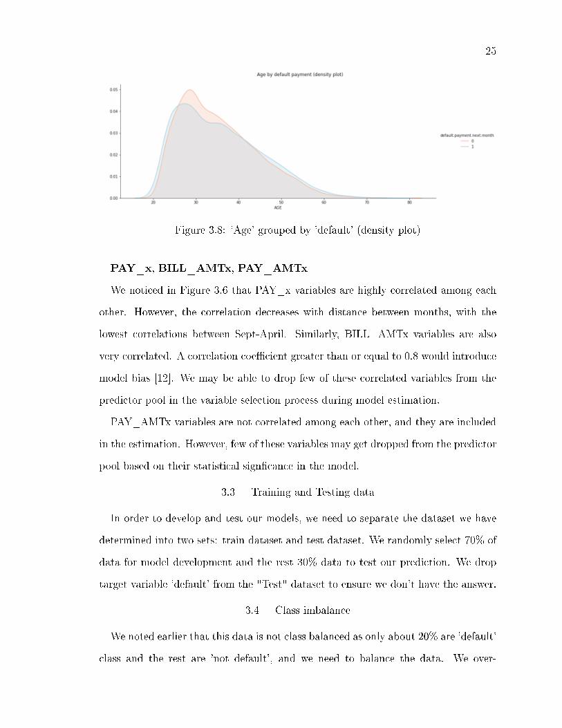
Based on the density plot in Figure 3.8, the distributions suggest that for a given
age the likelihood of default or not-default is almost same; the distributions are very
similar, except the age 30 population may have higher default rate. Overall, this
variable does not seem to provide a lot of information in the classi�cation prediction.
However, we plan to include it in the model estimation, and during the estimation
process we can measure the signi�cance of this variable and may decide to not include
in the �nal model.
25
Figure 3.8: 'Age' grouped by 'default' (density plot)
PAY_x, BILL_AMTx, PAY_AMTx
We noticed in Figure 3.6 that PAY_x variables are highly correlated among each
other. However, the correlation decreases with distance between months, with the
lowest correlations between Sept-April. Similarly, BILL_AMTx variables are also
very correlated. A correlation coe�cient greater than or equal to 0.8 would introduce
model bias [12]. We may be able to drop few of these correlated variables from the
predictor pool in the variable selection process during model estimation.
PAY_AMTx variables are not correlated among each other, and they are included
in the estimation. However, few of these variables may get dropped from the predictor
pool based on their statistical sign�cance in the model.
3.3 Training and Testing data
In order to develop and test our models, we need to separate the dataset we have
determined into two sets: train dataset and test dataset. We randomly select 70% of
data for model development and the rest 30% data to test our prediction. We drop
target variable 'default' from the "Test" dataset to ensure we don't have the answer.
3.4 Class imbalance
We noted earlier that this data is not class balanced as only about 20% are 'default'
class and the rest are 'not default', and we need to balance the data. We over-

26
sample the training data by up-sampling the default data. We use SMOTE algorithm
(Synthetic Minority Oversampling Technique) [13] for this purpose. The SMOTE
algorithm creates synthetic samples from the minor class, in this case 'default', by
randomly selecting one of the k-nearest-neighbors [13]. This way it does not create
copies of the minor class but it is creates similar new observations.

CHAPTER 4: MODEL ESTIMATIONS AND RESULTS
This chapter describes the model estimation process and analyzes prediction re-
sults. We develop and implement a parametric model - Logistic Regression, and
nonparametric models - Decision Tree, Random Forest and Arti�cial Neural Network
(ANN) on the balanced training data.
The model estimation process follows a systematic approach to model development
that includes the following steps:
1. Apply a benchmark model with randomly selected hyper-parameter values to
the training set and review the results. A benchmark result provides a reference
to any additional steps we take to improve the model performance.
2. Apply a hyper-parameter optimization approach, GridSearchCV [14], to opti-
mize hyper-parameters for the models to improve performance.
3. Apply a recursive variable elimination approach to drop variables based on their
importance in the estimation.
4. Examine key statistics for individual variables, check whether parameter esti-
mates have intuitive signs from business perspectives, and see if we can still
drop any insigni�cant variables based on their p-value
5. Propose the �nal model to implement on the training data
6. Review model results using performance metrics such as Accuracy, Confusion
Matrix, ROC curve, AUC.
In this research we use machine learning libraries such as scikit-learn [14], Ten-
sorFlow [15], and other open-source machine learning libraries, to develop and test

28
various model estimation and implementations. These libraries feature various re-
gression, clustering and classi�cation algorithms. We implemented several classi�-
cation algorithms from these libraries by developing codes in Python programming
languages. Use of these libraries is also helpful as they are designed to interoperate
with other Python numerical (NumPy, Panda), scienti�c (SciPy), and visualization
(seaborn, matplotlib) libraries.
4.1 Logistic regression model
This section proposes a Logistic regression model to predict if a customer would
default or not based on the given set of customer attributes. We start with applying a
benchmark logistic regression model and continually apply changes, such as predictor
variable pool, hyper-parameter optimization, to determine the �nal model.
Benchmark logistic regression
We applied a benchmark logistic regression on the training data set, mentioned in
section 3.4, and the following results show the model provides an accuracy of 55.77%.
At this point, the model is not very accurate. However, if we review the confusion
matrix in Figure 4.1 and ROC curve in Figure 4.2, we notice that it is showing a true
positive rate better than the false positive rate, etc. Also, F1-score also seems to be
pretty good. This shows the model is directionally correct but the accuracy can be
improved.

29
Figure 4.1: Confusion Matrix for the benchmark logistic regression model
Figure 4.2: ROC curve and AUC score for the benchmark logistic regression model
Tuning the hyper-parameters
In this step, we set the model to the best combination of hyper-parameters. We
apply an optimization approach for hyper-parameters tuning. In this approach an
exhaustive search over speci�ed parameter values are performed and the model is
evaluated by k-fold cross-validation. We used "GridSearchCV" package from "scikit-
learn" library [14] to perform the hyper-parameter tuning. The best parameters,
shown below, are selected to be used in the model.
Be-

30
low is the model performance on the test data after tuning the hyper-parameter.
We notice a signi�cant improvement in model performance. Accuracy is up by
15%, and AUC and F1-Score are also greater.
Variable selection
In this step, we remove variables based on their signi�cance in explaining the re-
sponse variable. We �rst apply a recursive variable elimination approach to determine
the reduced set of variables. We then apply our model again and look at the p-value
of coe�cients to further eliminate any variables with p-value greater than or equal to
0.05.
In recursive variable elimination algorithm [14], we specify the desired number of
variables to be included in the �nal set. In this approach, we select variables by
recursively selecting smaller and smaller sets of variables. First, the model is trained
on the initial set of variables and the least important variable is removed from the
current set. This step is recursively repeated on the smaller set until the desired
number of variables to select is reached [14]. We applied these algorithms using
"sklearn.feature_selection" package. We started with 22 variables, and wanted to
have the reduced set with 20 variables.
The output from the algorithm is as below:
The 'False' value suggests removal of the variables, 'LIMIT_BAL' and 'BILL_AMT4',

31
from the current predictor pool. We remove these two variables and apply and esti-
mate out logistic regression model on the reduced variable set. The parameter esti-
mation is shown in Figure 4.3. We notice that variables, 'PAY_5', 'BILL_AMT3',
'BILL_AMT5', and 'BILL_AMT6', have p-value greater than 0.05. We remove these
variables from the predictor list and select this model as our �nal logistic regression
model.
Figure 4.3: Model parameter estimate on the reduced predictor pool
The �nal logistic regression model
We apply �nal logistic regression model based on the �nal set of variable pool and
calculate the prediction results on the test data. Below is the best hyper-parameters

32
set used in the model and the performance results, and Figure 4.3, Figure 4.4 show
the confusion matrix and the ROC curve.
We notice an improvement on all metrics when compared to results from the model
before applying the variable selection approach.
Figure 4.4: Confusion matrix for the �nal logistic regression model
33
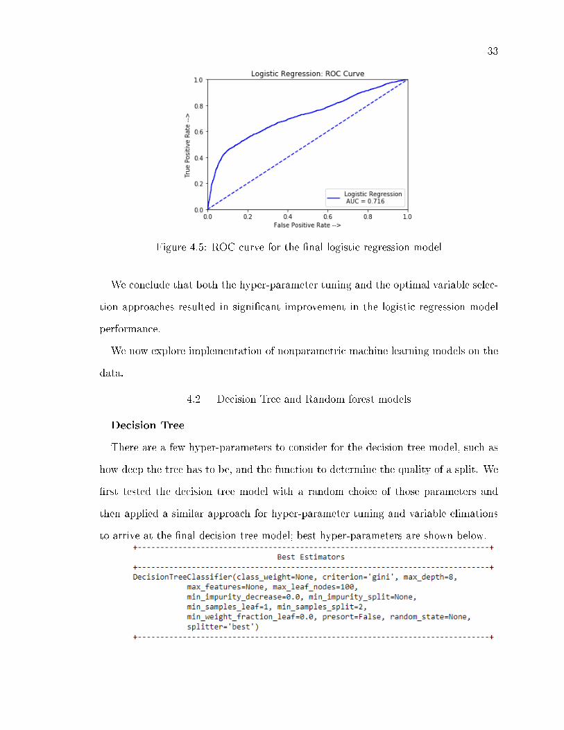
Figure 4.5: ROC curve for the �nal logistic regression model
We conclude that both the hyper-parameter tuning and the optimal variable selec-
tion approaches resulted in signi�cant improvement in the logistic regression model
performance.
We now explore implementation of nonparametric machine learning models on the
data.
4.2 Decision Tree and Random forest models
Decision Tree
There are a few hyper-parameters to consider for the decision tree model, such as
how deep the tree has to be, and the function to determine the quality of a split. We
�rst tested the decision tree model with a random choice of those parameters and
then applied a similar approach for hyper-parameter tuning and variable elimations
to arrive at the �nal decision tree model; best hyper-parameters are shown below.

34
The results from the Decision Tree model below shows higher Accuracy value,
higher AUC score and higher F1-score when compared to the Logistic Regression
model.
Figure 4.6 shows the Decision Tree model created using the training data. As we
can see, the tree model is very easy to use and imagine, but as discussed in Chapter
3 it is easy to fall into the trap of over�tting. For this reason, it is common to use
ensembles such as Random Forest to avoid this risk.
Figure 4.6: A Decision Tree model for the credit card default problem

35
Random Forest
Following is the best hyper-parameter selected for the algorithm following the ap-
proach mentioned in the logistic regression model development.
The results below suggest that the Random Forest show higher AUC score and
F1-score when compared with the results from the Decision Tree. After running the
Decision Tree few times we notice that the Decision Tree provides di�erent results at
each run. Unlike the Decision Tree, the Random Forest seemed to be very stable and
provided consistent results.
Arti�cial Neural Network (ANN)
We put a lot of e�orts in specifying search space for the hyper-parameter optimiza-
tion but could not see very good performance results with the ANN model on this
data. Also, it took the most time to run this model.
We can see that ANN has better Accuracy than our Benchmark model but overall

36
the performance is not so good when compared with the results from other models in
this study.
4.3 Models' performance results
Table 4.1 and Figure 4.7 show the results from di�erent models. Random Forest
seems to provide overall the best results on this data. Decision Tree results are very
close but we observed that results are not very stable, the model provided di�erent
results with a slight change in hyper-parameters. Random Forest showed very stable
results and is not very sensitive to hyper-parameters. ANN did not perform well on
this data.
The results seem to be reasonable, we are able to achieve over 80% accuracy with
a couple of models. However, some aspects of predictions need to be improved to be
used for a practical purpose.
Table 4.1: Models' performance results

37
Figure 4.7: ROC curves for various models
The models were evaluated on "accuracy" on each iteration of estimation opti-
mization. As a part of a future research, we may look into setting a speci�c objective
function to direct the model estimation in a speci�c direction. For instance, given
a very good economic outlook, the bank may have more appetite for risk and may
decide to be more inclined to minimize false negatives and less inclined to minimize
false positives. And if the bank predicts that the economic outlook is very good or the
asset quality of the customer on the books are not very good, it may want to restrict
credit and false negative may become more relevant. In other words, an improvement
to this approach would be to de�ne a speci�c cost function, which would take into
consideration any speci�c goals, to produce very practically applicable predictions.

CHAPTER 5: SUMMARY AND FUTURE RESEARCH
This thesis provides a systematic model development approach to statistical and
machine learning models to model a practical credit risk problem to predict customers
who would potentially default. The research applies and studies industry's most
popular tool - logistic regression - for such default probability related problem, and
also applies other newer nonparametric, machine learning algorithms to investigate
their applicability.
The thesis establishes the motivation, foundation and model development frame-
work for investigating the proposed research. It provides the theory on various models,
model evaluation to establish the context for the readers and foundation leading to
the development of these models for the problem.
The research provides an extensive exploratory data analyses to provide insight into
the data; the study included univariate analyses on variables, analyzed the response
of target variable to individual predictors, and analyzed correlation within variables
to suggest variable elimations to determine the pool of predictor variables. We also
determined training and testing data sets and balanced the training data based on
the response variable before using it in the model estimation process.
We estimated four models, Logistic Regression, Decision Tree, Random Forest,
and ANN, and reviewed their results using performance metrics such as Accuracy,
Confusion Matrix, ROC curve/ AUC-Score, and F1-Score. We found that overall
Random Forest provides the most stable and best predictions.
On the technical point of view, we provided a very systematic process of develop-
ing the models, which makes the model easy to implement in the practical setting.
However, we do think that certain aspects of the model estimation can be enhanced

39
to improve the models' prediction to be used for a practical purpose. We would like
to propose those enhancements as part of a future research.
The future work in this research may include:
1. Considering a card default data that includes information on macroeconomic
variables to build such models. Inclusion of macroeconomic variables will allow
for a more relevant prediction, and would allow for creating forecasts for multiple
di�erent scenarios - baseline (most likely scenario), economically adverse (stress
scenarios).
2. Including additional model evaluation approaches such as sensitivity analysis,
error attribution analysis, and back-testing analysis.
3. Analyzing variable selection by applying the credit risk domain knowledge. Re-
lying completely on the data and not applying business sense may steer the
estimation process in the wrong direction.
4. Developing a speci�c cost function, which takes into account the speci�c pre-
diction goal, to evaluate the models.
40
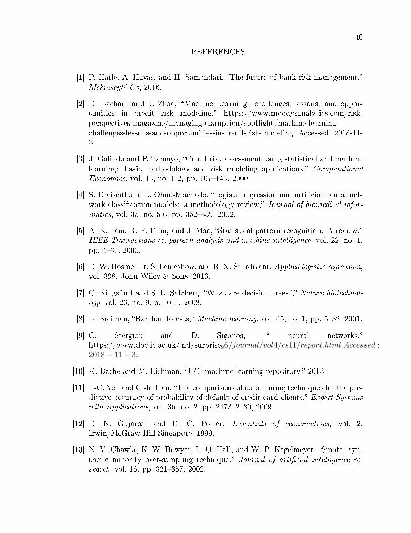
REFERENCES
[1] P. Härle, A. Havas, and H. Samandari, �The future of bank risk management,�Mckinsey& Co, 2016.
[2] D. Bacham and J. Zhao, �Machine Learning: challenges, lessons, and oppor-tunities in credit risk modeling.� https://www.moodysanalytics.com/risk-perspectives-magazine/managing-disruption/spotlight/machine-learning-challenges-lessons-and-opportunities-in-credit-risk-modeling. Accessed: 2018-11-3.
[3] J. Galindo and P. Tamayo, �Credit risk assessment using statistical and machinelearning: basic methodology and risk modeling applications,� Computational
Economics, vol. 15, no. 1-2, pp. 107�143, 2000.
[4] S. Dreiseitl and L. Ohno-Machado, �Logistic regression and arti�cial neural net-work classi�cation models: a methodology review,� Journal of biomedical infor-
matics, vol. 35, no. 5-6, pp. 352�359, 2002.
[5] A. K. Jain, R. P. Duin, and J. Mao, �Statistical pattern recognition: A review,�IEEE Transactions on pattern analysis and machine intelligence, vol. 22, no. 1,pp. 4�37, 2000.
[6] D. W. Hosmer Jr, S. Lemeshow, and R. X. Sturdivant, Applied logistic regression,vol. 398. John Wiley & Sons, 2013.
[7] C. Kingsford and S. L. Salzberg, �What are decision trees?,� Nature biotechnol-
ogy, vol. 26, no. 9, p. 1011, 2008.
[8] L. Breiman, �Random forests,� Machine learning, vol. 45, no. 1, pp. 5�32, 2001.
[9] C. Stergiou and D. Siganos, � neural networks.�https://www.doc.ic.ac.uk/ nd/surprise96/journal/vol4/cs11/report.html.Accessed :2018− 11− 3.
[10] K. Bache and M. Lichman, �UCI machine learning repository,� 2013.
[11] I.-C. Yeh and C.-h. Lien, �The comparisons of data mining techniques for the pre-dictive accuracy of probability of default of credit card clients,� Expert Systems
with Applications, vol. 36, no. 2, pp. 2473�2480, 2009.
[12] D. N. Gujarati and D. C. Porter, Essentials of econometrics, vol. 2.Irwin/McGraw-Hill Singapore, 1999.
[13] N. V. Chawla, K. W. Bowyer, L. O. Hall, and W. P. Kegelmeyer, �Smote: syn-thetic minority over-sampling technique,� Journal of arti�cial intelligence re-
search, vol. 16, pp. 321�357, 2002.

41
[14] F. Pedregosa, G. Varoquaux, A. Gramfort, V. Michel, B. Thirion, O. Grisel,M. Blondel, P. Prettenhofer, R. Weiss, V. Dubourg, et al., �Scikit-learn: Ma-chine learning in python,� Journal of machine learning research, vol. 12, no. Oct,pp. 2825�2830, 2011.
[15] M. Abadi, P. Barham, J. Chen, Z. Chen, A. Davis, J. Dean, M. Devin, S. Ghe-mawat, G. Irving, M. Isard, et al., �Tensor�ow: a system for large-scale machinelearning.,� in OSDI, vol. 16, pp. 265�283, 2016.