Electronic copy available at: http://ssrn.com/abstract=2773991

Predicting Baseline for Analysis of Electricity Pricing

Taehoon KimDongeun LeeJaesik Choi

Anna SpurlockAlex Sim

Annika ToddKesheng Wu

Lawrence Berkeley National LaboratoryOne Cyclotron Road, Berkeley, CA 94720

DISCLAIMERThis document was prepared as an account of work sponsored by the United States Government. While

this document is believed to contain correct information, neither the United States Government nor anyagency thereof, nor the Regents of the University of California, nor any of their employees, makes any war-ranty, express or implied, or assumes any legal responsibility for the accuracy, completeness, or usefulnessof any information, apparatus, product, or process disclosed, or represents that its use would not infringeprivately owned rights. Reference herein to any specific commercial product, process, or service by its tradename, trademark, manufacturer, or otherwise, does not necessarily constitute or imply its endorsement, rec-ommendation, or favoring by the United States Government or any agency thereof, or the Regents of theUniversity of California. The views and opinions of authors expressed herein do not necessarily state orreflect those of the United States Government or any agency thereof or the Regents of the University ofCalifornia.

Electronic copy available at: http://ssrn.com/abstract=2773991

Predicting Baseline for Analysis of Electricity Pricing

Taehoon Kim1, Dongeun Lee1, Jaesik Choi1, Anna Spurlock2, Alex Sim2, Annika Todd2, andKesheng Wu2

2Lawrence Berkeley National Laboratory, Berkeley CA, USA1Ulsan National Institute of Science and Technology, Ulsan, Korea

March 30, 2016

Abstract

To understand the impact of new pricing structure on residential electricity demands, we need abaseline model that captures every factor other than the new price. The standard baseline is a randomizedcontrol group, however, a good control group is hard to design. This motivates us to devlop data-drivenapproaches. We explored many techniques and designed a strategy, named LTAP, that could predict thehourly usage years ahead. The key challenge in this process is that the daily cycle of electricity demandpeaks a few hours after the temperature reaching its peak. Existing methods rely on the lagged variablesof recent past usages to enforce this daily cycle. These methods have trouble making predictions yearsahead. LTAP avoids this trouble by assuming the daily usage profile is determined by temperature andother factors. In a comparison against a well-designed control group, LTAP is found to produce accuratepredictions.

1 Introduction

With measurements recorded for most customers in a service territory at hourly or more frequent intervals,advanced metering infrastructure (AMI) captures electricity consumption in unprecedented spatial and tem-poral detail. This vast and fast growing stream of data, together with cutting-edge data science techniquesand behavioral theories, enables behavior analytics: novel insights into patterns of electricity consumptionand their underlying drivers [Costa and Kahn, 2013, Todd et al., 2014].

As electricity cannot be easily stored, electricity generation must match consumption. When the demandexceeds the generation capacity, a blackout would occur, typically during the time when consumers needelectricity the most [Joskow, 2001, Wolak, 2003]. Because increasing generation capacity is expensive andrequires years of time to implement, regulators and utility companies have devised a number of pricingschemes intended to discourage unnecessary consumption during peak demand periods.

To measure the effectiveness of a pricing policy on the peak demand, one can analyze electricity usagedata generated from AMI. Our work focuses on extracting baseline models of household electricity usagefor a behavior analytics study [Cappers et al., 2013, Costa and Kahn, 2013, Todd et al., 2014]. The baselinemodels would ideally capture the pattern of household electricity usage including all feastures except thenew pricing schemes. There are numerous challenges in establishing such a model. For example, there aremany features that could affect the usage of electricity, and many of these features, such as the purchase of

1

new equipement, is information not available to us. Other features, such as outdoor temperature, are known;but their impact is difficult to capture in simple functions.

Although this work shares some similarities with works on forecasting electricity demands and prices [Sug-anthi and Samuel, 2012, Bianco et al., 2009, Taylor and McSharry, 2007], there are a number of importantdifferences. The fundamental difference between a baseline model and a forecast model is that the baselinemodel needs to capture the core behavior that persist for a long time, while the forecast model typically aimsto forecast for the next few cycles of the time series in question. Typically, techniques that make forecastsfor years into the future are based on highly aggregated time series with month or year as time steps [Al-fares and Nazeeruddin, 2002, Bianco et al., 2009], whereas those that work on time series with shorter timesteps typically focus on making forecasts for the next day or the next few hours [Cottet and Smith, 2003,Oldewurtel et al., 2010, Panagiotelis and Smith, 2008, Taylor, 2010].

In the specific case that has motivated our work, the overall objective is to study the impacts of pricingpolicies. The process of designing these pricing schemes, recruiting participants for a pilot study, imple-menting the pricing schemes, and monitoring the impacts have taken a few years. The baseline model isbased on observed consumption prior to the implementation of the new pricing schemes, and applied topredict what consumer behavior would have been without the pricing changes. This is challenging becausethe baseline model not only captures intraday electricity usage but also needs to be applicable for years.Furthermore, in preliminary tests, we have noticed that the impact of the pricing schemes is weaker than theimpact of other factors such as temperature, therefore, the baseline model must be able to incorporate theoutdoor temperature, which has a complex relationship with the electricity demand.

This work examines a number of methods for developing the baseline models that could satisfy the aboverequirements. We use a large set of AMI data to exercise these methods and evaluate their relative strengths.The bulk of data in this work is hourly electricity usage from randomly chosen samples of households froma region of the US where the electricity usage is highest in the afternoon and evening during the monthsof May through August. The current work extracts the baseline models for average behavior of differentcustomer groups, not behavior specific to any individual household.

In the remainder of this paper, we briefly present the background and related work in Section 2 anddescribe the residential electricity usage data used in this study in Section 3. We also present some analysiswith conventional statistical methods in Section 3. We describe the methods used to extract the new typebaseline in Section 4 and discuss the output from these methods in Sections 5 and 6. A short summary isprovided in Section 7.

2 Application Driver

Energy management has become an important problem all around the world. The recent deployment ofresidential AMI makes hourly electricity consumption data available for research, which offers a uniqueopportunity to understand the electricity usage patterns of households. In particular, understanding howand when households use electricity is essential to regulators for increasing the efficiency of power distri-bution networks and enabling appropriate electricity pricing. One concrete objective from several currentpricing studies is to design new rules and structures to reduce the peak demand and therefore level out totalelectricity usage [Espey and Espey, 2004, Todd et al., 2014].

The influx of massive amounts of electricity data from AMI has led to a variety of research on energybehavior such as electricity consumption segmentation [Chicco et al., 2004, Figueiredo et al., 2005, Verduet al., 2006, Chicco et al., 2006, Tsekouras et al., 2007, Smith et al., 2012, Kwac et al., 2014], forecastingand load profiling [Espinoza et al., 2005, Irwin et al., 1986, Flath et al., 2012], and targeting customers for

2

an air-conditioning demand response program to maximize the likelihood of savings [Kwac and Rajagopal,2013].

An important tool for this problem is classifying and representing different households with differentload profiles [Capasso et al., 1994, Flath et al., 2012, Kwac et al., 2014]. Accurately identifying the loadprofiles will allow the researchers to associate observed electricity usage with consumer energy behavior.Load profiling could identify policy relevant energy lifestyle segmentation strategies, which can lead tobetter energy policy, improve program effectiveness, increase the accuracy of load forecasting, and createbetter program evaluation methods [Kwac et al., 2014].

Accurate prediction or load forecasting of electricity usage is very important for the industry [Nogaleset al., 2002, Ramchurn et al., 2012]. For example, long-term usage forecasting for more than one year aheadis important for capacity planning and infrastructure investments. Short-term forecasting is used in the day-ahead electricity market, determining available demand response, and increasing demand side flexibility. Wecan broadly divide these forecasting techniques into black-box techniques and white-box techniques. Theblack-box approaches focus on what could be extracted from data, typically based on statistical and machinelearning methods [Alfares and Nazeeruddin, 2002, Edwards et al., 2012, Espinoza et al., 2005, Irwin et al.,1986, Nogales et al., 2002, Ramchurn et al., 2012, Swan and Ugursal, 2009]. For example, some authorsprefer supervised machine learning methods such as support vector machines [Chen et al., 2004, Humeauet al., 2013], some use statistical models such as dynamic regression [Nogales et al., 2002], while othersadvocate for neural networks and artificial intelligence approaches [Ramchurn et al., 2012]. Typically, thesemethods transform the time series of historical data into a time scale such that the predictions are made forthe next time step or the next few time steps.

White-box approaches are typically based on some understanding of the relationship between somecause and its direct effect. For example, becuase increased outdoor temperature leads to increased indoortemperature, which in turn leads people to turn on their airconditioners, one might come up with a modelrelating outdoor temperature and electricity usage, and then try to fit the parameters of the model using theobserved data. However, such a model most likely would not be able to capture all relevant features, becausesome of the features, such as length of the day, have weak or unclear effect on electricity usage, and others,such as number of occupants in the building, clearly affect the eletricity usage but their values are unknownor their impact on electricity usage is multifacted or unknown [Borgeson, 2014, Fels, 1986, Rabl and Rialhe,1992]. For this reason, many researchers refer to these models as “gray-box” models because these modelsalways contain a certain amount of unexplained features left as “errors.”

Household electricity usage depends on many features beyond what was mentioned above, for example,appliances in the house, the energy behavior of the occupants, the time of day, day of the week, seasons, andso on [Cappers et al., 2013, Todd et al., 2012]. Some of the existing prediction models focus on aggregateddemand and therefore could parameterize many factors affecting the usage of an individual household [Swanand Ugursal, 2009]. From the study of earlier models, we learned that a household’s electricity usage isstrongly periodic, in that the daily electricity usage repeats every day and every week. Given any twoconsecutive days, their usage patterns are very similar to each other; given any two consecutive weeks, theirelectricity uses are also similar to each other. Throughout a year, the overall electricity usage follows thepattern of seasonal temperature change. To accurately predict electricity usage, we need to capture all thesefactors in our own models.

3

3 Dataset

Our electricity usage data was collected through a well-designed randomized control trial [Cappers et al.,2013]. It has hourly electricity consumption records of individual households for three years. The unitof electricity is in kilowatt-hour (KWh). The total number of hourly data points is 160,125,432, fromwhich we focus on data generated during the summers, which accounts for most of electricity usage (fromJune 1 to August 31), yielding 41,698,080 data records. The data records from three years are labelled by(T −1, T, T +1), where year T −1 corresponds to the year when the electricity has a fixed price throughoutthe day, and the new prices are used in year T and T + 1.

3.1 Groups

The households involved in this study are divided into a number of different groups, in this work, we onlyuse three of them, the Control group, the Passive group and the Active group. Following the general designof a randomized controll trial, the Control group is a random selected set of households that are meant to beused as the baseline [Costa and Kahn, 2013, Concato et al., 2000]. In later discussion, this group is labelledas Control. This control group is unaware of the study and stays with the previously available fixed-pricescheme throughout the testing period∗. The other two groups are generally referred to as the treatmentgroup.

The treatment groups use a time-based price, where during the peak-usage hours, 3PM to 7PM in theregion of this study, the per KWh charge is higher than the rest of the day. In the Active group, householdshave to opt in to the new pricing scheme offered. While the households in the Passive group are informedof their participatioin in the new price trial and offered a chance to opt out of the trial.

As in a typically consumer bahvior study, the response rate of the households invited to participate in thenew price trial, only a small fraction of the invitees actually opted in. To avoid the imbalance among the threegroups, we randomly selected about 1600 households from each of the three groups. We dropped householdsthat do not have measurement data for the whole duration of the study. The number of households droppedis relatively small.

3.2 Overall statistics

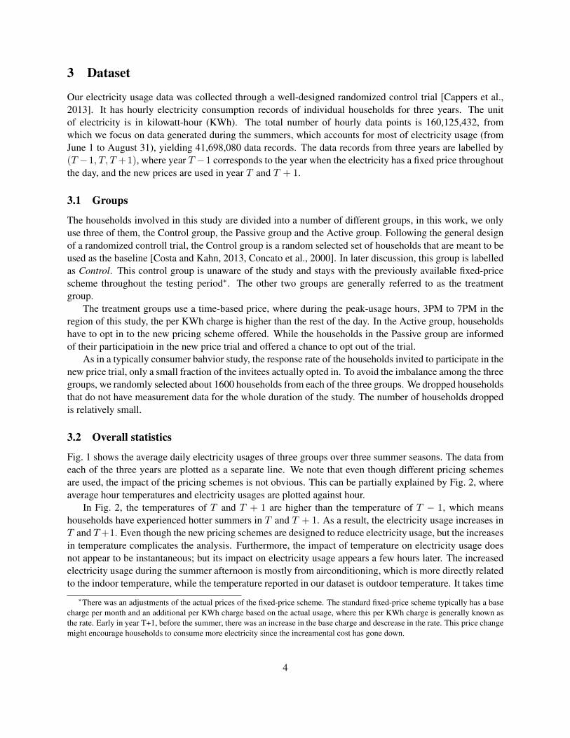
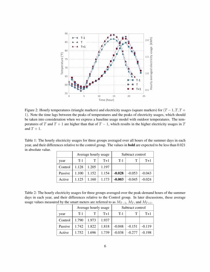
Fig. 1 shows the average daily electricity usages of three groups over three summer seasons. The data fromeach of the three years are plotted as a separate line. We note that even though different pricing schemesare used, the impact of the pricing schemes is not obvious. This can be partially explained by Fig. 2, whereaverage hour temperatures and electricity usages are plotted against hour.

In Fig. 2, the temperatures of T and T + 1 are higher than the temperature of T − 1, which meanshouseholds have experienced hotter summers in T and T + 1. As a result, the electricity usage increases inT and T+1. Even though the new pricing schemes are designed to reduce electricity usage, but the increasesin temperature complicates the analysis. Furthermore, the impact of temperature on electricity usage doesnot appear to be instantaneous; but its impact on electricity usage appears a few hours later. The increasedelectricity usage during the summer afternoon is mostly from airconditioning, which is more directly relatedto the indoor temperature, while the temperature reported in our dataset is outdoor temperature. It takes time∗There was an adjustments of the actual prices of the fixed-price scheme. The standard fixed-price scheme typically has a base

charge per month and an additional per KWh charge based on the actual usage, where this per KWh charge is generally known asthe rate. Early in year T+1, before the summer, there was an increase in the base charge and descrease in the rate. This price changemight encourage households to consume more electricity since the increamental cost has gone down.

4

Year T-1

Jun 08 Jun 22 Jul 06 Jul 20 Aug 03 Aug 17 Aug 312

4

6

8

10

12

14

16

Daily

ene

rgy

usag

e(KW

h)

ControlPassiveActive

Year T

Jun 08 Jun 22 Jul 06 Jul 20 Aug 03 Aug 17 Aug 312

4

6

8

10

12

14

16Da

ily e

nerg

y us

age(

KWh)

ControlPassiveActive

Year T+1

Jun 08 Jun 22 Jul 06 Jul 20 Aug 03 Aug 17 Aug 312

4

6

8

10

12

14

16

Daily

ene

rgy

usag

e(KW

h)

ControlPassiveActive

Figure 1: Daily electricity usages of three groups for year (T − 1, T, T + 1).

for the increased outdoor temperature to impact the indoor temperature. Additionally, residents of a housetypically return from work in late afternoon, which increase the number of occupants in a household.

Because there is no obvious differences from Figs. 1 and 2, we conclude that the influence of commonfeatures such as season, outdoor temperature, day of the week and so on are much stronger than the featuresthat distinguish the groups. This means the baseline models have to be very accurate in order to recognizethe different groups. We will discuss these methods carefully in Section 4.

5

0 5 10 15 20 25Time (hour)

55

60

65

70

75

80

85

90

Tem

pera

ture

(°F)

T-1TT+1

0.5

1.0

1.5

2.0

Hour

ly a

vera

ged

elec

trici

ty u

sage

(kW

h)

T-1TT+1

Figure 2: Hourly temperatures (triangle markers) and electricity usages (square markers) for (T − 1, T, T +1). Note the time lags between the peaks of temperatures and the peaks of electricity usages, which shouldbe taken into consideration when we express a baseline usage model with outdoor temperatures. The tem-peratures of T and T + 1 are higher than that of T − 1, which results in the higher electricity usages in Tand T + 1.

Table 1: The hourly electricity usages for three groups averaged over all hours of the summer days in eachyear, and their differences relative to the control group. The values in bold are expected to be less than 0.021in absolute value.

Average hourly usage Subtract control

year T-1 T T+1 T-1 T T+1

Control 1.128 1.205 1.197

Passive 1.100 1.152 1.154 -0.028 -0.053 -0.043

Active 1.125 1.160 1.173 -0.003 -0.045 -0.024

Table 2: The hourly electricity usages for three groups averaged over the peak-demand hours of the summerdays in each year, and their differences relative to the Control group. In later discussions, these averageusage values measured by the smart meters are referred to as MT−1, MT , and MT+1.

Average hourly usage Subtract control

year T-1 T T+1 T-1 T T+1

Control 1.790 1.973 1.937

Passive 1.742 1.822 1.818 -0.048 -0.151 -0.119

Active 1.752 1.696 1.739 -0.038 -0.277 -0.198

6

3.3 Comparison against the control group

In the tradition of randomized controlled trials, our dataset contains a control group. This control group isa valid counterfactual group and can provide a baseline for group-wise comparisons using a RandomizedEncouragement Design (RED) evaluation methodology [Todd et al., 2012]. However, we are interested indeveloping a new baseline methodology that does not rely on a randomized control group [Horwitz andFeinstein, 1979, Liddle et al., 1996]. We are interested in developing such a methodology for two reasons:(i) we would eventually like to use our technique to build a baseline for each household individually, whichnecessitates the development of new baseline models that do not rely on a control group counterfactual;(ii) it is often the case that programs, such as the pricing programs used in this paper, are implemented byelectricity providers without a randomized evaluation methodology. It is often the case that randomizationis either impractical, too expensive, or hampered by regulatory requirements. For this reason, it is extremelyvaluable to have a methodology that can be used to evaluate program effectiveness without relying on ran-domization. Therefore, we will be using this dataset in order to demonstrate such a methodology. We willuse the control group as a comparison group in order to validate the baseline methodology we develop, butwill use only the households in the treatment group that self-selected into treatment. If these householdswere compared directly to the control group, one would be concerned about self-selection bias. Using anaccurate baseline methodology is one potential way to avoid such a bias, by allowing for the estimation ofthe effect of the pricing scheme within those households that self-selected into the study.

Looking first at the broad changes in consumption across the groups. Tables 1 and 2 contain the averagehourly electricity consumption for all hours of a day and peak-demand hours, respectively. The values inTable 1 is averaged over all hours and all days of the summer months in each year, while the values inTable 2 is averaged over the peak-demand hours of each summer day. From these numbers, we see that theaverage hourly usages are higher in year T and year T+1. However, the increases of the two treatment groupsare smaller than that of the control group. Relative to the control group, the treatment groups have reducedelectricity consumption. This is particularly true during the peak-demand hours as shown in Table 2. Theseobserved changes match the design goal of the new pricing schemes.

In order to underline why a baseline method such as the one we develop is needed, we show herethe extent of the self-selection bias that exists if one were simply to compare the self-selected treatmenthouseholds to the control households. To do this we examine if the differences in year T-1 (before theintroduction of the treatments) are within the expected confidence intervals.

The standard deviations of hourly usage values for all households are all about 0.85 (KWh)† and eachof the group has about 1600 households, therefore, we expect the confidence interval of the these averagevalues to be about 0.85/

√1600 = 0.021. For a control group to be considered as properly selected, the

differences between the various groups before the introduction of the treatments should be less than 0.021,however among the two relevant difference values in year T-1 only one has a absolute value less than 0.021 inTable 1. This suggests that the three groups are not well randomized, and self-selection bias of the treatmentgroups could be strongly present in the data. We propose that the baseline method we develop is a solutionto this problem.

3.4 Differences among the groups

Next we directly compare the time series of the average hourly usage of each group to understand theirdifferences. For this test, we have selected to compare time series with the Kolmogorov-Smirnov test (KStest) [Conover and Conover, 1980]. Given two time series, the KS test measures the distance between their†The actual values are 0.83 for Year T-1, 0.85 for year T, and 0.91 for year T+1.

7

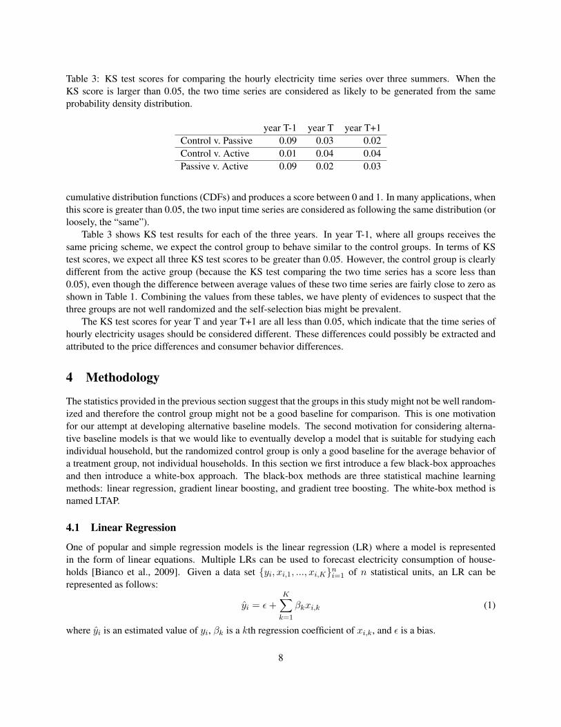
Table 3: KS test scores for comparing the hourly electricity time series over three summers. When theKS score is larger than 0.05, the two time series are considered as likely to be generated from the sameprobability density distribution.

year T-1 year T year T+1Control v. Passive 0.09 0.03 0.02Control v. Active 0.01 0.04 0.04Passive v. Active 0.09 0.02 0.03

cumulative distribution functions (CDFs) and produces a score between 0 and 1. In many applications, whenthis score is greater than 0.05, the two input time series are considered as following the same distribution (orloosely, the “same”).

Table 3 shows KS test results for each of the three years. In year T-1, where all groups receives thesame pricing scheme, we expect the control group to behave similar to the control groups. In terms of KStest scores, we expect all three KS test scores to be greater than 0.05. However, the control group is clearlydifferent from the active group (because the KS test comparing the two time series has a score less than0.05), even though the difference between average values of these two time series are fairly close to zero asshown in Table 1. Combining the values from these tables, we have plenty of evidences to suspect that thethree groups are not well randomized and the self-selection bias might be prevalent.

The KS test scores for year T and year T+1 are all less than 0.05, which indicate that the time series ofhourly electricity usages should be considered different. These differences could possibly be extracted andattributed to the price differences and consumer behavior differences.

4 Methodology

The statistics provided in the previous section suggest that the groups in this study might not be well random-ized and therefore the control group might not be a good baseline for comparison. This is one motivationfor our attempt at developing alternative baseline models. The second motivation for considering alterna-tive baseline models is that we would like to eventually develop a model that is suitable for studying eachindividual household, but the randomized control group is only a good baseline for the average behavior ofa treatment group, not individual households. In this section we first introduce a few black-box approachesand then introduce a white-box approach. The black-box methods are three statistical machine learningmethods: linear regression, gradient linear boosting, and gradient tree boosting. The white-box method isnamed LTAP.

4.1 Linear Regression

One of popular and simple regression models is the linear regression (LR) where a model is representedin the form of linear equations. Multiple LRs can be used to forecast electricity consumption of house-holds [Bianco et al., 2009]. Given a data set yi, xi,1, ..., xi,Kni=1 of n statistical units, an LR can berepresented as follows:

yi = ε+K∑k=1

βkxi,k (1)

where yi is an estimated value of yi, βk is a kth regression coefficient of xi,k, and ε is a bias.

8

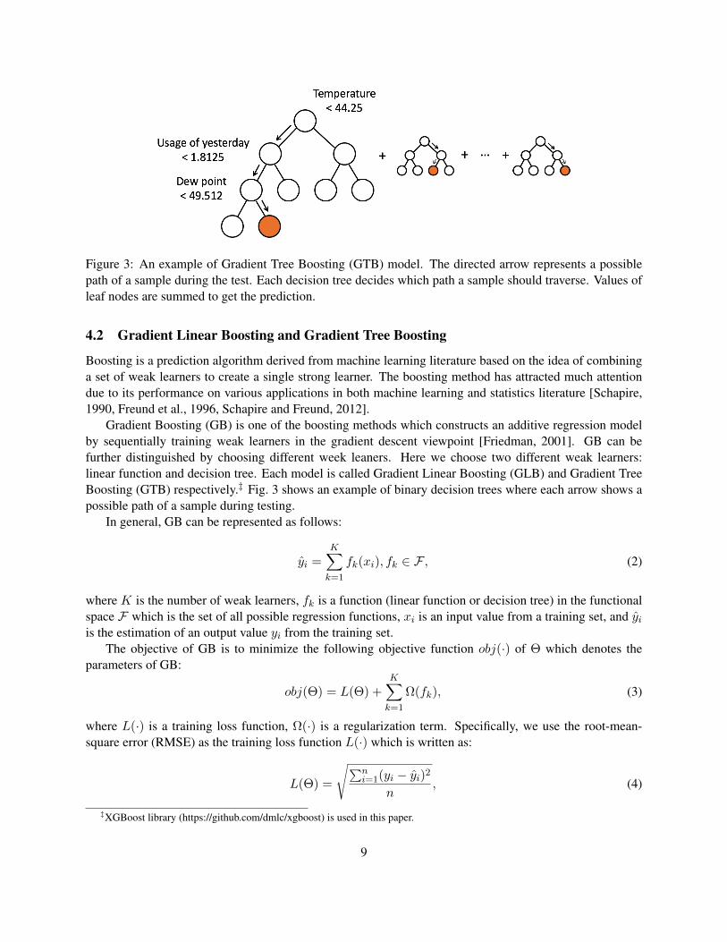
Figure 3: An example of Gradient Tree Boosting (GTB) model. The directed arrow represents a possiblepath of a sample during the test. Each decision tree decides which path a sample should traverse. Values ofleaf nodes are summed to get the prediction.

4.2 Gradient Linear Boosting and Gradient Tree Boosting

Boosting is a prediction algorithm derived from machine learning literature based on the idea of combininga set of weak learners to create a single strong learner. The boosting method has attracted much attentiondue to its performance on various applications in both machine learning and statistics literature [Schapire,1990, Freund et al., 1996, Schapire and Freund, 2012].

Gradient Boosting (GB) is one of the boosting methods which constructs an additive regression modelby sequentially training weak learners in the gradient descent viewpoint [Friedman, 2001]. GB can befurther distinguished by choosing different week leaners. Here we choose two different weak learners:linear function and decision tree. Each model is called Gradient Linear Boosting (GLB) and Gradient TreeBoosting (GTB) respectively.‡ Fig. 3 shows an example of binary decision trees where each arrow shows apossible path of a sample during testing.

In general, GB can be represented as follows:

yi =K∑k=1

fk(xi), fk ∈ F , (2)

where K is the number of weak learners, fk is a function (linear function or decision tree) in the functionalspace F which is the set of all possible regression functions, xi is an input value from a training set, and yiis the estimation of an output value yi from the training set.

The objective of GB is to minimize the following objective function obj(·) of Θ which denotes theparameters of GB:

obj(Θ) = L(Θ) +K∑k=1

Ω(fk), (3)

where L(·) is a training loss function, Ω(·) is a regularization term. Specifically, we use the root-mean-square error (RMSE) as the training loss function L(·) which is written as:

L(Θ) =

√∑ni=1(yi − yi)2

n, (4)

‡XGBoost library (https://github.com/dmlc/xgboost) is used in this paper.

9

where n is the number of elements in the training set. We employ hourly training datasets (xi, yi) forexperiments.

4.3 Linear Relation between Temperature and Aggregated Power (LTAP)

Next, we describe the white-box model that is effective in our tests. It is well-known that the electricityconsumption depends on temperature [Fels, 1986]. Generally, this relationship is between the electricityusage of a whole day and the average temperature of that day [Rabl and Rialhe, 1992, Bacher and Madsen,2011, Borgeson, 2014]. In this work, we propose a simple strategy to make predictions of hourly usagebased on this relationship between the daily electricity usage and the average daily temperature. Next, weprovide a brief explanation of the rationale for this method before describing the method.

As we see from Figure 2, the relationship between outdoor temperature and the hourly electricity usageis complex, but the daily electricity usage and the average outdoor temperature is relatively straightforward.Since this work is primarily concerned about the peak usages during the summer when airconditioner usescause the electricity demand to peak in the later afternoon. From the earlier studies on the residentialelectricity usage, we know there is a significant amount of constant demands from refrigerators, electricwater heaters, water pumps, and so on. We assume that this constant usage is the minimum hourly usageduring a day and is fixed during the summer season being considered for this work. The usage that is beyondthe minimum varies from hour to hour, we call this portion the variable electricity usage. For the regionwhere this data is from, we assume the primary demand for this variable usage is from the airconditionersand therefore is related to the outdoor temperature.

The reason that the daily variable electricity usage is likely a simple function of the average daily tem-perature can be stated as follows. The higher outdoor temperature causes heat to enter into a house andincreases the indoor temperature. When the indoor temperature rises to a certain threshold, the aircondi-tioner starts to cool the room. There is a delay between the rise of outdoor temperature and the rise of theindoor temperature because of the insulation of the house, however, during the warm period of the day, thehigher the average temperature causes more heat to enter the house, and more electric power is needed tocool the house. Therefore, we expect the aggregate variable electricity usage per day to have a relatively sim-ple relation with the average outdoor temperature. From the research literature and our own tests presentedin the next section, we see that this is true. In fact, we have a set of linear functions relating the aggregatevariable electricity usage and the average outdoor temperature. We will use these linear relationships toforecast the total variable electricity usage from the reported outdoor temperature values.

To distribute the aggregate daily usage to hourly usage values, we make the simple assumption thatthe profile of daily usage per household remains the same, and scale the variable hourly electricity usageproportional to the change in the aggregated usage. Next, we give a more precise definition of the procedurewe call LTAP.

Given a summer day in year T or year T+1, we compute the average temperature t1 of the day fromthe hour temperature values. Call this the prediction day. Look for a summer day in year T-1 with theclosest average temperature t0. Call this day the reference day. Let the 24 hourly electricity usage beh0[i], i = 0, . . . , 23. Let b0 ≡ minh0[i] and a0 ≡

∑(h0[i] − b0). Let s denote the slope of the linear

relation between a0 and t0. We compute a1 as follows

a1 = a0 + s(t1 − t0). (5)

We assign the hourly electricity usage as follows

h1[i] = b0 + (h0[i]− b0)a1/a0. (6)

10

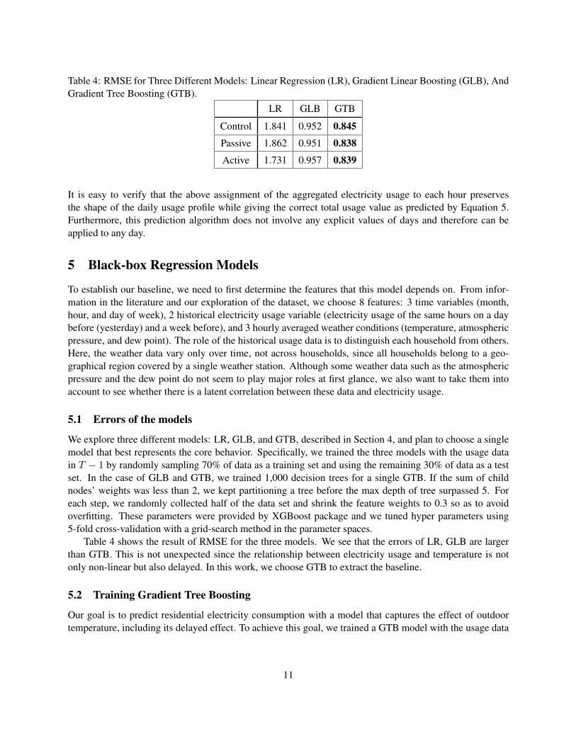
Table 4: RMSE for Three Different Models: Linear Regression (LR), Gradient Linear Boosting (GLB), AndGradient Tree Boosting (GTB).

LR GLB GTB

Control 1.841 0.952 0.845

Passive 1.862 0.951 0.838

Active 1.731 0.957 0.839

It is easy to verify that the above assignment of the aggregated electricity usage to each hour preservesthe shape of the daily usage profile while giving the correct total usage value as predicted by Equation 5.Furthermore, this prediction algorithm does not involve any explicit values of days and therefore can beapplied to any day.

5 Black-box Regression Models

To establish our baseline, we need to first determine the features that this model depends on. From infor-mation in the literature and our exploration of the dataset, we choose 8 features: 3 time variables (month,hour, and day of week), 2 historical electricity usage variable (electricity usage of the same hours on a daybefore (yesterday) and a week before), and 3 hourly averaged weather conditions (temperature, atmosphericpressure, and dew point). The role of the historical usage data is to distinguish each household from others.Here, the weather data vary only over time, not across households, since all households belong to a geo-graphical region covered by a single weather station. Although some weather data such as the atmosphericpressure and the dew point do not seem to play major roles at first glance, we also want to take them intoaccount to see whether there is a latent correlation between these data and electricity usage.

5.1 Errors of the models

We explore three different models: LR, GLB, and GTB, described in Section 4, and plan to choose a singlemodel that best represents the core behavior. Specifically, we trained the three models with the usage datain T − 1 by randomly sampling 70% of data as a training set and using the remaining 30% of data as a testset. In the case of GLB and GTB, we trained 1,000 decision trees for a single GTB. If the sum of childnodes’ weights was less than 2, we kept partitioning a tree before the max depth of tree surpassed 5. Foreach step, we randomly collected half of the data set and shrink the feature weights to 0.3 so as to avoidoverfitting. These parameters were provided by XGBoost package and we tuned hyper parameters using5-fold cross-validation with a grid-search method in the parameter spaces.

Table 4 shows the result of RMSE for the three models. We see that the errors of LR, GLB are largerthan GTB. This is not unexpected since the relationship between electricity usage and temperature is notonly non-linear but also delayed. In this work, we choose GTB to extract the baseline.

5.2 Training Gradient Tree Boosting

Our goal is to predict residential electricity consumption with a model that captures the effect of outdoortemperature, including its delayed effect. To achieve this goal, we trained a GTB model with the usage data

11

yeste

rday

weekbefore

temperature

hour

air pressu

re

dew point

dayofw

eekmonth

010002000300040005000600070008000

f-sco

re

controlactive1active2passive1passive2passive1&2

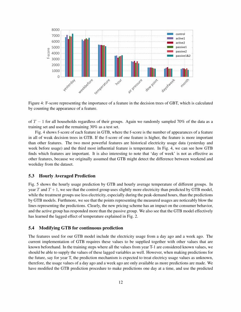
Figure 4: F-score representing the importance of a feature in the decision trees of GBT, which is calculatedby counting the appearance of a feature.

of T − 1 for all households regardless of their groups. Again we randomly sampled 70% of the data as atraining set and used the remaining 30% as a test set.

Fig. 4 shows f-score of each feature in GTB, where the f-score is the number of appearances of a featurein all of weak decision trees in GTB. If the f-score of one feature is higher, the feature is more importantthan other features. The two most powerful features are historical electricity usage data (yesterday andweek before usage) and the third most influential feature is temperature. In Fig. 4, we can see how GTBfinds which features are important. It is also interesting to note that ‘day of week’ is not as effective asother features, because we originally assumed that GTB might detect the difference between weekend andweekday from the dataset.

5.3 Hourly Averaged Prediction

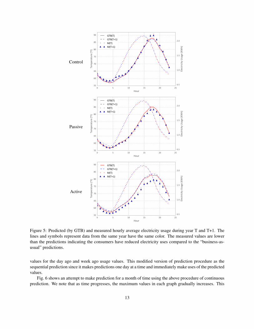
Fig. 5 shows the hourly usage prediction by GTB and hourly average temperature of different groups. Inyear T and T + 1, we see that the control group uses slightly more electricity than predicted by GTB model,while the treatment groups use less electricity, especially during the peak-demand hours, than the predictionsby GTB models. Furthmore, we see that the points representing the measured usages are noticeably blow thelines representing the predictions. Clearly, the new pricing scheme has an impact on the consumer behavior,and the active group has responded more than the passive group. We also see that the GTB model effectivelyhas learned the lagged effect of temperature explained in Fig. 2.

5.4 Modifying GTB for continuous prediction

The features used for our GTB model include the electricity usage from a day ago and a week ago. Thecurrent implementation of GTB requires these values to be supplied together with other values that areknown beforehand. In the training steps where all the values from year T-1 are considered known values, weshould be able to supply the values of these lagged variables as well. However, when making predictions forthe future, say for year T, the prediction mechanism is expected to treat electricy usage values as unknown,therefore, the usage values of a day ago and a week ago are only available as more predictions are made. Wehave modified the GTB prediction procedure to make predictions one day at a time, and use the predicted

12

Control

0 5 10 15 20 25Hour

55

60

65

70

75

80

85

90

Tem

pera

ture

(°F)

0.5

1.0

1.5

2.0

Elec

trici

ty U

sage

(KW

h)

GTB(T)GTB(T+1)M(T)M(T+1)

Passive

0 5 10 15 20 25Hour

55

60

65

70

75

80

85

90

Tem

pera

ture

(°F)

0.5

1.0

1.5

2.0

Elec

trici

ty U

sage

(KW

h)

GTB(T)GTB(T+1)M(T)M(T+1)

Active

0 5 10 15 20 25Hour

55

60

65

70

75

80

85

90

Tem

pera

ture

(°F)

0.5

1.0

1.5

2.0

Elec

trici

ty U

sage

(KW

h)

GTB(T)GTB(T+1)M(T)M(T+1)

Figure 5: Predicted (by GTB) and measured hourly average electricity usage during year T and T+1. Thelines and symbols represent data from the same year have the same color. The measured values are lowerthan the predictions indicating the consumers have reduced electricity uses compared to the “business-as-usual” predictions.

values for the day ago and week ago usage values. This modified version of prediction procedure as thesequential prediction since it makes predictions one day at a time and immediately make uses of the predictedvalues.

Fig. 6 shows an attempt to make prediction for a month of time using the above procedure of continuousprediction. We note that as time progresses, the maximum values in each graph gradually increases. This

13

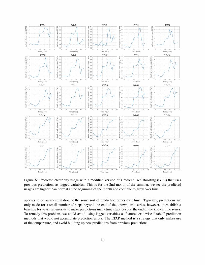
Figure 6: Predicted electricity usage with a modified version of Gradient Tree Boosting (GTB) that usesprevious predictions as lagged variables. This is for the 2nd month of the summer, we see the predictedusages are higher than normal at the beginning of the month and continue to grow over time.

appears to be an accumulation of the some sort of prediction errors over time. Typically, predictions areonly made for a small number of steps beyond the end of the known time series, however, to establish abaseline for years requires us to make predictions many time steps beyond the end of the known time series.To remedy this problem, we could avoid using lagged variables as features or devise “stable” predictionmethods that would not accumulate prediction errors. The LTAP method is a strategy that only makes useof the temperature, and avoid building up new predictions from previous predictions.

14

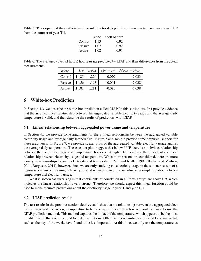
Table 5: The slopes and the coefficients of correlation for data points with average temperature above 65Ffrom the summer of year T-1.

slope coeff of corrControl 1.13 0.92Passive 1.07 0.92Active 1.02 0.91

Table 6: The averaged (over all hours) hourly usage predicted by LTAP and their differences from the actualmeasurements.

group DT DT+1 MT − PT MT+1 − PT+1

Control 1.185 1.220 0.020 -0.023

Passive 1.156 1.193 -0.004 -0.038

Active 1.181 1.211 -0.021 -0.038

6 White-box Prediction

In Section 4.3, we describe the white-box prediction called LTAP. In this section, we first provide evidencethat the assumed linear relationship between the aggregated variable electricity usage and the average dailytemperature is valid, and then describe the results of predictions with LTAP.

6.1 Linear relationship between aggregated power usage and temperature

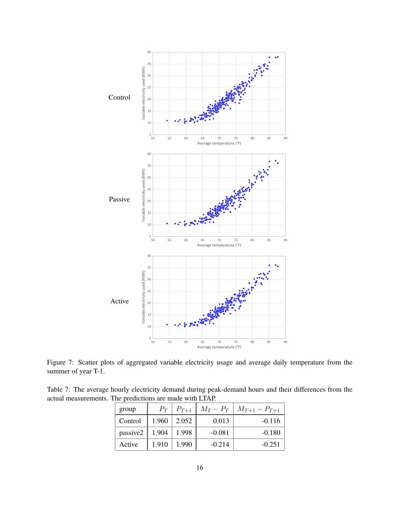
In Section 4.3 we provide some arguments for the a linear relationship between the aggregated variableelectricity usage and average daily temperature. Figure 7 and Table 5 provide some empirical support forthese arguments. In Figure 7, we provide scatter plots of the aggregated variable electricity usage againstthe average daily temperature. These scatter plots suggest that below 65F, there is no obvious relationshipbetween the electricity usage and temperature, however, at higher temperatures there is clearly a linearrelationship between electricity usage and temperature. When more seasons are considered, there are morevariety of relationships between electricity and temperature [Rabl and Rialhe, 1992, Bacher and Madsen,2011, Borgeson, 2014], however, since we are only studying the electricity usage in the summer season of aregion where airconditioning is heavily used, it is unsurprising that we observe a simpler relation betweentemperature and electricity usage.

What is somewhat surprising is that coefficients of correlation in all three groups are above 0.9, whichindicates the linear relationship is very strong. Therefore, we should expect this linear function could beused to make accurate predictions about the electricity usage in year T and year T+1.

6.2 LTAP prediction results

The test results in the previous section clearly establishes that the relationship between the aggregated elec-tricity usage and the average temperature to be piece-wise linear, therefore we could attempt to use theLTAP prediction method. This method captures the impact of the temperature, which appears to be the mostreliable feature that could be used to make predictions. Other factors we initially suspected to be impactful,such as the day of the week, have found to be less important. At this time, we only use the temperature as

15

Control

50 55 60 65 70 75 80 85 90Average temperature (°F)

5

10

15

20

25

30

35

40

Varia

ble

elec

trici

ty u

sed

(KW

h)

Passive

50 55 60 65 70 75 80 85 90Average temperature (°F)

5

10

15

20

25

30

35

40

Varia

ble

elec

trici

ty u

sed

(KW

h)

Active

50 55 60 65 70 75 80 85 90Average temperature (°F)

5

10

15

20

25

30

35

40

Varia

ble

elec

trici

ty u

sed

(KW

h)

Figure 7: Scatter plots of aggregated variable electricity usage and average daily temperature from thesummer of year T-1.

Table 7: The average hourly electricity demand during peak-demand hours and their differences from theactual measurements. The predictions are made with LTAP.

group PT PT+1 MT − PT MT+1 − PT+1

Control 1.960 2.052 0.013 -0.116

passive2 1.904 1.998 -0.081 -0.180

Active 1.910 1.990 -0.214 -0.251

16

Control

0 5 10 15 20 25Hour

55

60

65

70

75

80

85

90

Tem

pera

ture

(°F)

0.5

1.0

1.5

2.0

Elec

trici

ty U

sage

(KW

h)

LTAP(T)LTAP(T+1)M(T)M(T+1)

Passive

0 5 10 15 20 25Hour

55

60

65

70

75

80

85

90

Tem

pera

ture

(°F)

0.5

1.0

1.5

2.0

Elec

trici

ty U

sage

(KW

h)

LTAP(T)LTAP(T+1)M(T)M(T+1)

Active

0 5 10 15 20 25Hour

55

60

65

70

75

80

85

90

Tem

pera

ture

(°F)

0.5

1.0

1.5

2.0

Elec

trici

ty U

sage

(KW

h)

LTAP(T)LTAP(T+1)M(T)M(T+1)

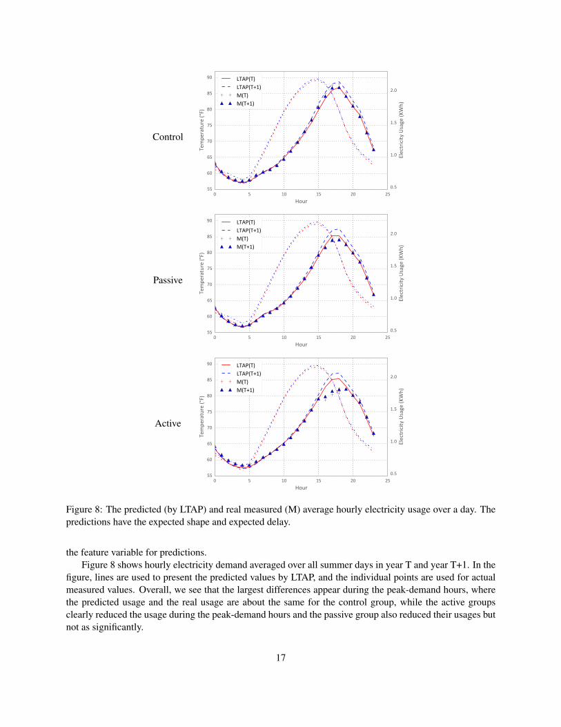
Figure 8: The predicted (by LTAP) and real measured (M) average hourly electricity usage over a day. Thepredictions have the expected shape and expected delay.

the feature variable for predictions.Figure 8 shows hourly electricity demand averaged over all summer days in year T and year T+1. In the

figure, lines are used to present the predicted values by LTAP, and the individual points are used for actualmeasured values. Overall, we see that the largest differences appear during the peak-demand hours, wherethe predicted usage and the real usage are about the same for the control group, while the active groupsclearly reduced the usage during the peak-demand hours and the passive group also reduced their usages butnot as significantly.

17

Tables 6 and 7 provide more quantitative measures of the reduction in electricity demand. The LTAPbaseline predictions are able to capture the impact of temperature, we can regard the difference betweenthe predicted values and the actual measurements as the “true” measure of energy reduction due to thenew pricing schemes. Overall, we see the impact of the new pricing scheme on the overall daily usage isrelatively small, while the impact on the usage during peak-demand hours is quite significant.

From Table 7 we see that the active group is able to reduce their usage during the peak-demand hoursmuch more than the passive groups. The reduction by the active groups during the peak-demand hoursreaches almost 20%, which is very signficant. There are some households that reduce the usage duringpeak-demand hours by as much as 40%. This indicates that the new pricing structure is effective in reducingelectricity usage during peak-demand hours. It is possible that these active participants choose to opt inbecause they are better able to respond to the incentives provided by new pricing scheme.

A unexpected observation from this table is that all groups reduced electricity usage in year T+1, even thecontrol group. This particular change in the behavior of the control group appears to explain the decreasesin the reduction observed in year T+1 in Table 2. Based on he values in Table 2, we have speculated that thedecrease in reduction of electricity usage indicates the active participants have become tired of respondingto the changing price during the day. The new baseline with LTAP seems to suggest a new interpretation ofthe consumer behavior. The control group must have heard about the new behavior of the active participantsand started to mimic their behavior even though there is no incentive for them to do so.

7 Summary and Future Work

We set out to study options of derive baseline models from data because the randomized control group ishard to design and is even impossible in some cases. Ultimately, we would like to design a strategy that couldgenerate baseline models for individual participants of a study, while the randomized control group can onlyserve as the baseline for a whole group. For this work, we have chosen a data set from a well-designed fieldstudy of residential electricity usage because it contains a control group that we could compare our baselinemodel against.

In this work, we explored a number of black-box approaches such as linear regression and GradientBoosting. Among these machine learning methods, we found Gradient Tree Boosting to be more effectivethan others. However, the most accurate GTB models are produced with lagged variables as features, forexample, the electricity usage a day before and a week before. In order to use the model established on datafrom year T-1 to make predictions for year T, the existing structure of the prediction procedure effectivelyrequires the actual usage data from year T in order to make predictions for values in year T. We have at-tempted to modify the prediction procedure to use the recently predictions in place of the actual measuredvalues, however the tests show that the prediction errors accumulated over time, leading to unrealistic pre-dictions a month or so into the summer season. This type of accumulation of prediction errors is commonto sequential prediction procedures for time series.

To address the above difficulty, we devised a number of white-box approaches. The method knownas LTAP is reported here. It is based on the fact that the aggregated variable electricity usage per day isaccurately described by a piece-wise linear function of average daily temperature. This fact allows us tomake predictions about the total daily electricity usage. By assuming the usage profile remains the sameduring the study, we are able to assign the hourly usage values from the aggregated daily usage. Thisapproach is shown to be self-consistent, that is the prediction procedure exactly reproduces the electricityusage in year T-1 and the prediction for the control in year T is very close to the actual measured values. Asone might expect, both treatment groups have reduced electricity usage during the peak-demand hours and

18

the active group reduced the usage more than the passive group.The analysis results also contain a unexpected revelation, the control group actually reduced its electric-

ity usages in year T+1, the second year after the introduction of the new pricing structures. Previously, usingthe randomized control group as the baseline, researchers have concluded that there was a decrease in thereduction of the electricity usage during the peak-demand hours. This decrease might be an indication thatthe new pricing scheme has lost its attractiveness. The new analysis results suggest alternate possibilities,for example, households might have acquired more energy efficient airconditioners, the change the fixedrate at the beginning of year T+1 might have make the consumers more concerned about their electricityusage, or participants of the control group might have adapted the behavior of the treatment groups.

The above hypothesis should be investigated and we are interested in further verify the effectiveness ofLTAP. One way to improve LTAP might be to capture additional features, such as the day of the week and soon. So far, we have only considered the average usages of groups, LTAP could be used to make predictionof individual household. We plan to exercise this feature, which might provide additional ways to verifythe new baseline model. From our tests on GTB, we noted that the prediction errors seem to accumulateover time, it is of great theoretical interest to study sequential prediction methods that would not accumulateprediction errors over time.

Acknowledgment

The authors gratefully acknowledge the helpful discussions with Sam Borgeson, Daniel Fredman, LieselHans, Ling Jin, and Sid Patel.

This work is supported in part by the Director, Office of Laboratory Policy and Infrastructure Man-agement of the U.S. Department of Energy under contract No. DE-AC02-05CH11231. This work is alsosupported by Basic Science Research Program through the National Research Foundation of Korea (NRF)grant funded by the Ministry of Science, ICT & Future Planning (MSIP) (NRF-2014R1A1A1002662) andthe NRF grant funded by the MSIP (NRF-2014M2A8A2074096).

References

Hesham K. Alfares and Mohammad Nazeeruddin. Electric load forecasting: Literature survey and classifi-cation of methods. International Journal of Systems Science, 33(1):23–34, January 2002.

Peder Bacher and Henrik Madsen. Identifying suitable models for the heat dynamics of buildings. Energyand Buildings, 43(7):1511–1522, 2011.

Vincenzo Bianco, Oronzio Manca, and Sergio Nardini. Electricity consumption forecasting in Italy usinglinear regression models. Energy, 34(9):1413–1421, 2009.

Sam Borgeson. Targeted Efficiency: Using Customer Meter Data to Improve Efficiency Program Outcomes.PhD thesis, UC Berkeley, 2014. Available at http://pqdtopen.proquest.com/pubnum/3686197.html and https://escholarship.org/uc/item/32q1w1sf.

A. Capasso, W. Grattieri, R. Lamedica, and A. Prudenzi. A bottom-up approach to residential load modeling.IEEE Transactions on Power Systems, 9(2):957–964, May 1994.

19

Peter Cappers, Annika Todd, Michael Perry, Bernard Neenan, and Richard Boisvert. Quantifying the im-pacts of time-based rates, enabling technology, and other treatments in consumer behavior studies: Pro-tocols and guidelines. Technical Report LBNL-6301E, Lawrence Berkeley National Laboratory, 2013.URL http://eetd.lbl.gov/sites/all/files/lbnl-6301e.pdf.

Bo-Juen Chen, Ming-Wei Chang, and Chih-Jen Lin. Load forecasting using support vector machines: Astudy on EUNITE competition 2001. IEEE Transactions on Power Systems, 19(4):1821–1830, 2004.

Gianfranco Chicco, Roberto Napoli, and Federico Piglione. Comparisons among clustering techniques forelectricity customer classification. IEEE Transactions on Power Systems, 21(2):933–940, 2006.

Gianfranco Chicco, Roberto Napoli, Federico Piglione, Petru Postolache, Mircea Scutariu, and CornelToader. Load pattern-based classification of electricity customers. IEEE Transactions on Power Sys-tems, 19(2):1232–1239, 2004.

John Concato, Nirav Shah, and Ralph I. Horwitz. Randomized, controlled trials, observational studies, andthe hierarchy of research designs. New England Journal of Medicine, 342(25):1887–1892, June 2000.

William Jay Conover and WJ Conover. Practical nonparametric statistics. Wiley New York, 1980.

Dora L. Costa and Matthew E. Kahn. Energy conservation ”nudges” and environmentalist ideology: Ev-idence from a randomized residential electricity field experiment. Journal of the European EconomicAssociation, 11(3):680–702, June 2013.

Remy Cottet and Michael Smith. Bayesian modeling and forecasting of intraday electricity load. Journalof the American Statistical Association, 98(464):839–849, 2003.

Richard E Edwards, Joshua New, and Lynne E Parker. Predicting future hourly residential electrical con-sumption: A machine learning case study. Energy and Buildings, 49:591–603, 2012.

James A. Espey and Molly Espey. Turning on the lights: A meta-analysis of residential electricity demandelasticities. Journal of Agricultural and Applied Economics, 36:65–81, 2004.

Marcelo Espinoza, Caroline Joye, Ronnie Belmans, and Bart De Moor. Short-term load forecasting, profileidentification, and customer segmentation: a methodology based on periodic time series. IEEE Transac-tions on Power Systems, 20(3):1622–1630, 2005.

Margaret F Fels. Prism: an introduction. Energy and Buildings, 9(1-2):5–18, 1986.

Vera Figueiredo, Fatima Rodrigues, Zita Vale, and Joaquim Borges Gouveia. An electric energy consumercharacterization framework based on data mining techniques. IEEE Transactions on Power Systems, 20(2):596–602, 2005.

Dipl-Wi-Ing Christoph Flath, Dipl-Wi-Ing David Nicolay, Tobias Conte, PD Dr Clemens van Dinther, andLilia Filipova-Neumann. Cluster analysis of smart metering data. Business & Information Systems Engi-neering, 4(1):31–39, 2012.

Yoav Freund, Robert E Schapire, et al. Experiments with a new boosting algorithm. In Proceedings ofInternational Conference on Machine Learning, volume 96, pages 148–156, 1996.

20

Jerome H Friedman. Greedy function approximation: A gradient boosting machine. Annals of statistics,pages 1189–1232, 2001.

Ralph I Horwitz and Alvan R Feinstein. Methodologic standards and contradictory results in case-controlresearch. The American journal of medicine, 66(4):556–564, 1979.

Samuel Humeau, Tri Kurniawan Wijaya, Matteo Vasirani, and Karl Aberer. Electricity load forecasting forresidential customers: Exploiting aggregation and correlation between households. In Proceedings ofSustainable Internet and ICT for Sustainability, pages 1–6. IEEE, 2013.

GW Irwin, W Monteith, and WC Beattie. Statistical electricity demand modelling from consumer billingdata. In IEE Proceedings C (Generation, Transmission and Distribution), volume 133, pages 328–335.IET, 1986.

Paul L Joskow. California’s electricity crisis. Oxford Review of Economic Policy, 17(3):365–388, 2001.

Jungsuk Kwac, June Flora, and Ram Rajagopal. Household energy consumption segmentation using hourlydata. IEEE Transactions on Smart Grid, 5(1):420–430, 2014.

Jungsuk Kwac and Ram Rajagopal. Demand response targeting using big data analytics. In Proceedings ofIEEE International Conference on Big Data, pages 683–690. IEEE, 2013.

Jeannine Liddle, Margaret Williamson, Les Irwig, and New South Wales. Method for evaluating research& guideline evidence. NSW Department of Health, 1996.

F. J. Nogales, J. Contreras, A. J. Conejo, and R. Espinola. Forecasting next-day electricity prices by timeseries models. IEEE Transactions on Power Systems, 17(2):342–348, May 2002.

F. Oldewurtel, A. Ulbig, A. Parisio, G. Andersson, and M. Morari. Reducing peak electricity demand inbuilding climate control using real-time pricing and model predictive control. In Proceeding of IEEEConference on Decision and Control, pages 1927–1932, December 2010.

Anastasios Panagiotelis and Michael Smith. Bayesian density forecasting of intraday electricity pricesusing multivariate skew t distributions. International Journal of Forecasting, 24(4):710–727, 2008. URLhttp://www.sciencedirect.com/science/article/pii/S0169207008001015.

A. Rabl and A. Rialhe. Energy signature models for commercial buildings: test with measured data andinterpretation. Energy and Buildings, 19(2):143–154, 1992. URL http://www.sciencedirect.com/science/article/pii/0378778892900085.

Sarvapali D. Ramchurn, Perukrishnen Vytelingum, Alex Rogers, and Nicholas R. Jennings. Putting the’smarts’ into the smart grid: A grand challenge for artificial intelligence. Communications of the ACM,55(4):86–97, April 2012.

Robert E Schapire. The strength of weak learnability. Machine learning, 5(2):197–227, 1990.

Robert E Schapire and Yoav Freund. Boosting: Foundations and algorithms. MIT press, 2012.

Brian Artur Smith, Jeffrey Wong, and Ram Rajagopal. A simple way to use interval data to segment residen-tial customers for energy efficiency and demand response program targeting. In Proceedings of ACEEESummer Study on Energy Efficiency in Buildings, 2012.

21

L. Suganthi and Anand A. Samuel. Energy models for demand forecasting – a review. Renewable andSustainable Energy Reviews, 16(2):1223–1240, 2012. URL http://www.sciencedirect.com/science/article/pii/S1364032111004242.

Lukas G. Swan and V. Ismet Ugursal. Modeling of end-use energy consumption in the residential sector: Areview of modeling techniques. Renewable and Sustainable Energy Reviews, 13(8):1819–1835, 2009.

J. W. Taylor and P. E. McSharry. Short-term load forecasting methods: An evaluation based on Europeandata. IEEE Transactions on Power Systems, 22(4):2213–2219, November 2007.

James W. Taylor. Triple seasonal methods for short-term electricity demand forecasting. European Jour-nal of Operational Research, 204(1):139–152, 2010. URL http://www.sciencedirect.com/science/article/pii/S037722170900705X.

Annika Todd, Michael Perry, Brian Smith, Michael J. Sullivan, Peter Cappers, and Charles A. Gold-man. Insights from smart meters: The potential for peak hour savings from behavior-based pro-grams. Technical Report LBNL-6598E, Lawrence Berkeley National Laboratory, 2014. URL http://escholarship.org/uc/item/2nv5q42n.

Annika Todd, Elizabeth Stuart, Steven R. Schiller, and Charles A. Goldman. Evaluation, measurement,and verification (EM&V) of residential behavior-based energy efficiency programs: Issues and rec-ommendations. Technical Report DOE/EE-0734, US Department of Energy, 2012. URL http://eetd.lbl.gov/sites/all/files/publications/behavior-based-emv.pdf.

George J Tsekouras, Nikos D Hatziargyriou, and Evangelos N Dialynas. Two-stage pattern recognitionof load curves for classification of electricity customers. IEEE Transactions on Power Systems, 22(3):1120–1128, 2007.

Sergio Valero Verdu, Mario Ortiz Garcia, Carolina Senabre, Antonio Gabaldon Marin, and FranciscoJ Garcıa Franco. Classification, filtering, and identification of electrical customer load patterns throughthe use of self-organizing maps. IEEE Transactions on Power Systems, 21(4):1672–1682, 2006.

Frank A Wolak. Diagnosing the California electricity crisis. The Electricity Journal, 16(7):11–37, 2003.

22