Predicting Account Receivables with Machine Learning

Predicting Account Receivables with Machine LearningAna Paula Appel*[email protected]

IBM ResearchSão Paulo, Brazil

Gabriel Louzada Malfatti*[email protected]

IBM ResearchSão Paulo, Brazil

Renato Luiz de Freitas Cunha*

[email protected] Research

São Paulo, Brazil

Bruno Lima*


São Paulo, Brazil

Rogerio de Paula*


São Paulo, Brazil

ABSTRACTBeing able to predict when invoices will be paid is valuable in mul-tiple industries and supports decision-making processes in mostfinancial workflows. However, due to the complexity of data re-lated to invoices and the fact that the decision-making process isnot registered in the accounts receivable system, performing thisprediction becomes a challenge. In this paper, we present a proto-type able to support collectors in predicting the payment of invoices.This prototype is part of a solution developed in partnership with amultinational bank and it has reached up to 81% of prediction accu-racy, which improved the prioritization of customers and supportedthe daily work of collectors. Our simulations show that adoptionof our model to prioritize the work o collectors saves up to ≈1.75million dollars per month. The methodology and results presentedin this paper will allow researchers and practitioners in dealing withthe problem of invoice payment prediction, providing insights andexamples of how to tackle issues present in real data.

KEYWORDSmachine learning, account receivables, feature engineering, payment,finance

ACM Reference Format:Ana Paula Appel, Gabriel Louzada Malfatti, Renato Luiz de Freitas Cunha,Bruno Lima, and Rogerio de Paula. 2020. Predicting Account Receivableswith Machine Learning. In KDD Workshop on Machine Learning in Finance(KDD MLF ’20). ACM, New York, NY, USA, 9 pages.

1 INTRODUCTIONThe invoice-to-cash process involves various steps, from invoicecreation to customer’s debt (payment) settlement or reconciliation.One key step of this process is the collection of accounts receivables.Accounts receivables (AR) refers to the invoices issued by a companyfor products or services already delivered but not yet paid for by itscustomers. Properly managing AR is a core accounting activity andconcern of any company, pertaining to its cash-flow.

Despite the widespread use and adoption of information tech-nologies in recent years across domain and industry applications,

Permission to make digital or hard copies of part or all of this work for personal orclassroom use is granted without fee provided that copies are not made or distributedfor profit or commercial advantage and that copies bear this notice and the full citationon the first page. Copyrights for third-party components of this work must be honored.For all other uses, contact the owner/author(s).KDD MLF ’20, August 23–27, 2020, San Diego, CA© 2020 Copyright held by the owner/author(s).

particularly machine learning techniques, there are still companiesthat manage internal processes in the same ways they did in the past:with paper and pencil.

In this work, we present a case study carried out in partnershipwith a multinational bank (hereafter also referred to as client). Inthis case study, we sought for innovative ways to proactively iden-tify overdue ARs with high probability of being paid such that itsmanagers and executives could take appropriate actions (such as,reaching out to those customers and collecting those ARs). As aninternational bank, it operates in multiple countries; however, thisproject focuses exclusively on its customers based in Latin Americaand the United States.

The collection activity is performed by analysts, also known ascollectors. Collectors are responsible for charging the bank’s cus-tomers (hereafter referred to as customers) and, in turn, improvingthese customers’ experience relative to the payment processes. In thebank, each collector deals with approximately a hundred customersand these customers are allocated according to the seniority levelof the collector, meaning that senior collectors are responsible forbigger accounts and contracts. In collecting ARs (i.e. the activityof charging customers), collectors receive daily a list prioritizingcustomers to contact. This list takes into account a customer’s debtbased on all of its overdue invoices. Nonetheless, it ignores thecustomer’s payment behavior, such as, whether this customer reg-ularly pays on time or not. Usually, customers are contacted at afixed schedule before due dates, irrespective of whether a particularcustomer regularly pays its invoices on time or not. Neither does itdifferentiate a recurrent from a sporadic payment behavior, such asan occasional financial problem faced by a customer. However, inthe end, all of this detailed information about customers’ paymentbehaviors lays in individual collectors’ minds, being utilized just inan ad-hoc manner.

Figure 1: Receivables over one month, distributed over the pay-ment data. Each point can have one or more invoices, with big-ger points representing a bigger number of invoices.

arX

iv:2

008.

0736

3v1

[cs

.LG

] 1

1 A

ug 2

020

KDD MLF ’20, August 23–27, 2020, San Diego, CA Ana P. Appel, Gabriel L. Malfatti, Renato Luiz de F. Cunha, Bruno Lima, and Rogerio de Paula

Figure 1 represents what collectors face every day, which is deal-ing with a large number of invoices from several clients in a month.Each bubble represents a set of invoices with the due date for thatday, the size of each bubble represents how many invoices are therein any particular day, potentially from different clients. The positionof the bubbles are the amount of money to be receive in a givenday. Looking only at that Figure, it might become hard to prioritizewhich clients should be contacted first. Such a representation leavesinformation out, such as which clients are more likely to pay late.Therefore, the easy route might be to go after the larger amounts ofmoney first, since collector performance is measured by the amountof money they recover. A larger sum of money does not necessar-ily represent higher risk clients, though. Hence, predicting invoicewhich invoices are most likely to be paid next can be a solution tobetter allocate resources, impacting positively cash flow estimation,essential to achieving financial stability.

In our research, we assert that by providing insights as to how toprioritize contacting clients based on the probability of late paymenthelps collectors make more effective and efficient decisions. Theobjective is to help them make more assertive and timely decisionsby means of focusing their collection actions on invoices that wouldhave a greater financial return, while at the same time focusing onthose most likely to make a payment. To this end, the system shouldprovide a personalized, ranked list of customers whom to contact,taking into account a collector’s own list of customers and theirpayment behavior.

Predictive modeling approaches are widely used in a number of re-lated domains, such as credit management and tax collection [1]. Theproblem of predicting invoice payment has been traditionally tackledusing statistical survival analysis methods, such as the proportionalhazards method [13]. Survival analysis is a statistical method foranalyzing the expected duration of time until one or more events hap-pen, such as death in biological organisms and failure in mechanicalsystems.

Dirick et al. [7] tested several survival analysis techniques incredit data from Belgian and Great Britain financial institutions.Survival analysis techniques were also used to model consumercredit risk [5, 6, 14]. The aforementioned pieces of work focus onpredicting when an event may occur, rather than whether it mayoccur or not. This aligns with our interest in analyzing time to anevent; thus, a survival analysis approach is a reasonable techniquefor tackling the problem at hand.

Smirnov [15] concluded that Random Survival Forests models,which additionally uses historical payment behavior of debtors, per-form better in ranking payment times of late invoices than traditionalCox Proportional Hazards models. Although the proportional haz-ards model is the most frequently used model for survival analysis,it still has a number of drawbacks, such as having a baseline haz-ard function which is uniform and proportional across the entirepopulation, as explained by Baesens et al. [2].

Invoice payment prediction could also be modeled as a classifica-tion problem, but there is just a small body of work that addressesthis problem. One of the few works that investigate this is the oneby Zeng et al. [19], where the authors formulate the problem as atraditional supervised classification and apply existing classifiers toit. They divided the clients into four different classes related to pay-ment delays: on time, 1-30 days, 31-60 days, and +60 days. These

classes are usually related to AR processes and counter measures foraddressing late invoices. Similarly, Bailey et al. [3] analyze severalstrategies for prioritizing collection calls and propose to use predic-tive modeling based on binary logistic regression and discriminativeanalysis to determine which customers to hand over to an outsidecollections agency for further collection processing.

Tater et al. [17] propose a different approach to the problem andinstead of predicting invoice in accounts receivable, they focus on ac-counts payable, working on invoices that were already delayed. Sim-ilarly, Younes [18] focuses on accounts payable case and attempts toaddress the problem of invoice processing time, understanding theoverdue invoices and the impact of delays in the invoice processing.Abe et al. [1], in addition, propose a new approach for optimallymanaging the tax and, more generally, debt collections processes atfinancial institutions.

The prototype herein described aims at devising and developinga tool employing state-of-the-art Artificial Intelligence (AI) algo-rithms and techniques for creating a ranked list of (potential) overdueaccounts for each collector, based on different criteria, such as thehighest probability of payment in the short-term, payment behaviorpatterns, and the like. It thus aims at optimizing collectors’ actionsand thus improving the payment rate of these accounts.

The key contributions of this paper are:

• The use of machine learning to predict with high accuracythe status of invoices (late or on time), allowing the bank tobetter estimate how much money will be delayed in cash andwork pro-actively to avoid late payments;

• The use of historical and temporal features to improve ac-curacy of models and an extensive comparison of MachineLearning models applied to this problem;

• An effective new way for ranking customers to be prioritizedby collectors not only by taking into account the volume ofmoney, but also the probability of being late;

• Our simulations show that adoption of our model to prioritizethe work of collectors saves up to ≈1.75 million dollars permonth.

The paper is organized as follows. Section 2 defines the problemformally. Section 3 characterizes the data set used in the work andthe ETL (Extract, Transform, Load) process. Section 4 shows themodeling approach applied in the problem and the results obtainedso far. Section 5 presents the prioritizing list proposed to client andthe simulations showing that the model and the new ranking areable to saving a large amount of money. Finally, Section 6 discussesoutcomes and concludes our work.

2 PROBLEM DEFINITIONIn AR collection, the ability of monitoring and collecting paymentsenables the prediction of payment behavior. Firms often use varioustypes of metrics to measure the performance of the collection process.One example is the average number of days overdue. Particularly inour case, the client is interested mainly in knowing the probabilitythat an invoice will be paid late or on time to then be able to betterprioritize the collection.

The problem of predicting an invoice payment is a typical clas-sification problem using supervised learning [11] where, given theoriginal client dataset, we need to extract invoices’ features to be

Predicting Account Receivables with Machine Learning KDD MLF ’20, August 23–27, 2020, San Diego, CA

Country # invoices # customers

United States 26,506 4,276Argentina 220 27Brazil 17,510 785Chile 11,634 324Colombia 16,302 514Ecuador 6 1Mexico 19,484 578

Table 1: Data distribution for Latin America and NorthAmerica shown by country. Some countries are very under-represented in the data, thus we aimed at building one modelfor all countries instead of a particular model for each country.

able to characterize each invoice with respect to labeled classes,building then a machine learning model to perform classification ofnew invoices.

In a more formal way, we can define our problem as follows:

DEFINITION 1. Let M = I ,Y be a set of pairs of invoices andtheir respective classes. Element Mm is represented by the pair⟨Im ,Ym⟩, with Im represented as a set of features A = a1,a2, . . . ,an ,and the class Ym having a binary value representing either a “late”or “on time” state for Im .

In order to prepare the dataset for the model training, we definedclass Ym for each invoice Im . The definition of class Ym as “on time”or “late” is done as follows:

Ym =

{on time, if payment at most 5 days from due datelate, otherwise

(1)

Thus, an invoice is considered overdue if payment occurs morethan 5 days after the due date. The main reason for considering thistime window is the time required to process payments in the clientsystem. This interval was elicited during one of the meetings wehad with client’s subject matter experts (SMEs) to understand theproblem, processes, and work flow of the collection activity.

3 DATA SOURCE AND ETLThe dataset received from the client has 91,562 invoices from 6countries from Latin America plus the United States, with 2,229customers over dates ranging from November 2018 to November2019. The distribution of invoices by country is presented in Table 1.Since we have some countries with low representativeness, afteranalyzing the payment behaviour of the countries with high repre-sentativeness in the dataset, we decided to develop only one modelfor all countries, instead of one model for each country.

The dataset only contains information about payments, specifi-cally about invoices. For instance, invoice value, country code, cus-tomer number, etc. One of important challenge of using this datasetis that it has no relevant information about customers. Therefore,information such as industry sector and balance sheets are missingfrom the dataset. The dataset only has a unique identifier used todifferentiate customers. Since the scope and time of the project does

not include gathering information about customers, and due to pri-vacy constraints, we decided to proceed with this anonymized data,and work only with invoice information.

One of the biggest challenges in projects such as the one describedhere, is how to transform the invoice data to enrich it with relevantfeatures in order to build a machine learning model. Being the resultof manual data processes, and as is usual with real datasets, we founda large number of missing values and incorrect data in several fieldsthat would be important for machine learning models. Additionally,the dataset was compiled from legacy systems of branches from allover the world, and the result of a data consolidation effort by theclient. In order to extract the most valuable features from the data,we performed several discussions with client’s SMEs and collectors,looking at previous literature on AR, and performed a thorough,detailed examination of the dataset.

We started with traditional invoice-level features, such as invoiceamount, issue date, due date, settled date, etc. In order to enrichour model with more significant information, we performed featureextraction to build the late invoice payment model.

We used historical data to create aggregate features that couldbring more meaning to our set of invoice-level features, as the use ofaggregate features increase significantly the amount of informationabout payment [19]. However, some of the features recommendedin the literature [19] did not work in our case, specially due tosome data related issues. One such example is the computation ofratios that, due to the amount of missing information in some fields,increased the number of invalid (such as null or NAN) values in thedata. Additionally, some features, such as a category that specifiedwhether an invoice was under dispute or not, had consistency issues,due to being manually entered information.

On the other hand, we incorporated some features related to therecent payments in order to capture customer behavior. Based onour careful analysis of the data, we observed that recent paymentsinfluence more in the payment behaviour than older payments. Inother words, the recent payment behavior of a customer has morepredictive power than the complete payment history. In this particularcase, we noticed that encoding whether a customer had paid eachof their last three invoices had more predictive power. In additionto that, we computed as features the percentage of paid invoices,payment frequency, number of contracts related to each invoice, andstandard deviation of late and outstanding invoices. The list bellowshows the constructed features as well as the respective descriptions.

• paid invoice: Value indicating whether the last invoice waspaid or not; where 1 means paid, 0 means not paid, and -1indicates null value (possibly due to this customer being afirst time customer).

• total paid invoices: Number of paid invoices prior to thecreation date of a new invoice of a customer.

• sum amount paid invoices: The sum of the base amount fromall the paid invoices prior to a new invoice for a customer.

• total invoices late: Number of invoices which were paid lateprior to the creation date of a new invoice of a customer.

• sum amount late invoices: The sum of the base amount fromall the paid invoices which were late prior to a new invoicefor a customer.


• total outstanding invoices: Number of the outstanding in-voices prior to the creation date of a new invoice of a cus-tomer.

• total outstanding late: Number of the outstanding invoiceswhich were late prior to the creation date of a new invoice ofa customer.

• sum total outstanding: The sum of the base amount from allthe outstanding invoices prior to a new invoice for a customer.

• sum late outstanding: The sum of the base amount from all theoutstanding invoices which were late prior to a new invoicefor a customer.

• average days late: Average days late of all paid invoices thatwere late prior to a new invoice for a customer.

• average days outstanding late: Average days late of all out-standing invoices that were late prior to a new invoice for acustomer

• standard deviation invoices late: Standard deviation of allinvoices that were paid late.

• standard deviation invoices outstanding late: Standard devi-ation of days late of all outstanding invoices that were lateprior to a new invoice for a customer.

• payment frequency difference: Amount of times the customerdid a payment. Intention here is to identify customers thatpayed more invoices (payment could be 30, 45, 60 days).

The next step in our ETL process was to handle missing values.We had to do this for invoices that did not have too much historicalinformation according to our features. One such case was that, ifwe had a null value for the total sum of invoices, we just replacedit with zero. However, in a few cases it was necessary to take intoconsideration what the feature meant and its representation. Foraverage days late, for example, we could not fill with zeros, as itwould be an indicative of good payment behavior. In such cases, weused the mean value of the feature as a replacement rule for missingones.

With the dataset cleaned up and properly set up, we could startto work in the best way to split the data into train and test sets. Toprevent data leakage, that is to create an accurate model to makepredictions on new data, unseen during training, we split our datasetconsidering time. Thus, the split into train and test sets was based ontime of invoice creation. For training, we considered data rangingfrom November 2018 to April 2019 and test from May 2019 to No-vember 2019. Table 2 presents in details the amount of invoices thatwe had in each sample of our dataset. As we can see, the distributionof invoices between late and on time is a somewhat imbalancedtowards late invoices, except that in the test set we have the samedistribution between late and on-time invoices.

Once we had the training set, we used cross-validation to tunehyper-parameters. The folds were separated using a time series split,based on invoice creation date. This is needed because we want thedistribution of data in the validation set to be as close as possible tothe data in the test set, so that performance measures in the validationset is predictive of performance in the test set. Therefore, a randomshuffle would be a bad option in this case, since it would mix morerecent invoices with older ones in both datasets, giving an advantageto the model during training and validation which would not bbereflected with new, unseen data.

4 MODELING APPROACHES AND RESULTSAs explained before, our problem was defined as a binary classifica-tion problem to predict whether an invoice will be paid on time orlate. Although we stated the problem as predicting classes, a widerange of models return probabilities instead of just labels. This iscrucial in order to do a prioritization list and rank customers withhigher chances of default. Also, since the model is planned to bedeployed in a client service that ultimately will need to retrain andupdate the model, it is important that we use a powerful model interms of scalability, while being able to handle missing values, andwith results that are easy to understand while being easy to retrain,so that non-machine learning experts could have a sense about whatis going on with the data and the model.

Most of features came from historical data, for example, sumamount late invoices, total invoices late and so on. In order to calcu-late these features for an invoice, we needed to define a maximumperiod of time that the system would consider to look back. This pe-riod is different from our trained dataset that defines which invoiceswe will consider. To define the best range of time to look back tocalculate the features, we created a parameter that we call windowsize, represented by the letter w . In short, window size will bethe number of months prior to an invoice that we will consider tocalculate our features values.

One might wonder why limit past data to a window, instead ofusing the complete, historical data. The problem is that, as timepasses, the statistical distribution of the features also changes andreduces the accuracy of the model, since all the models consideredwork on the assumption that data is independent, and identically-distributed. In the machine learning and predictive analytics realmthis is known as concept drift. Therefore, it is necessary to work withboundaries and to focus on getting information from the most recentpast, representing the most recent customer behavior.

In order to create a more robust model and to make sure that weare using the correct time range, we created ten datasets with wranging from 3 to 12 months to perform tests and see how manymonths do we need to consider. We decide to use as w values from3 months or above, because in our feature engineering we have afeature that looks at the three last payments that are mostly in the 3months range and we know that our data is very susceptible to datadrift and is susceptible to external changes, such as changes in theeconomy, politics, and policies.

We tested our data with six different classification methods: NaiveBayes, Logistic Regression, k-Nearest Neighbors (k-NN), RandomForest [4], Gradient Boosted Decision Trees (XGBoost) [8], DeepNeural Network based on the fastai library (DNN) [9]. For eachclassifier, we performed cross-validation for hyper-parameter selec-tion. Below, we describe how each model was built and the set ofhyper-parameters used for model selection.

Naive Bayes. We used a Gaussian Naive Bayes implementationof the scikit-learn 0.22 library. Due to the simplicity of the imple-mentation, we did not build a grid of hyper-parameters to searchthrough for this algorithm.

Logistic Regression. We used the Logistic Regression implemen-tation of the scikit-learn 0.22 library. Hyper-parameters for thismodel were (with parameters in bold representing the best values


Dataset invoices Late On Time Baseline Period

Train 71,545 61.17% 38.83% 61.17% 2018-11 - 2019-06Test 19,630 54.51% 45.49% 54.51% 2019-07 - 2019-11

Table 2: Data distribution for training and test sets. The classes are balanced and our baseline is close to 61%. We split the datausing time, since we cannot use future data to make predictions. We use 70% of available data to train the model and the other 30%we split in test and validation data. We did a time series split since the temporal characteristic of the that does not allow traditionalcross-validation method.

found by a cross-validated grid search): penalty chosen from [L1, L2],C (inverse of regularization strength) chosen from [0.5, 1, 5, 10, 20, 50],class weights chosen from [balanced,None], and maximum numberof iterations chosen from [10, 50, 100].

k-Nearest Neighbors. We used the k-Nearest Neighbors imple-mentation of the scikit-learn 0.22 library. For hyper-parameter search,we chose the number of neighbors from elements of the set {n : 29 ≤n < 100}, and the best number of neighbors found set to 49.

Gradient Boosted Decision Trees. We used the XGBoost libraryand performed a grid search for model selection. Hyper-parameterswere, with the parameters in bold representing the best found valuesfor each hyper parameter: learning rate was set to 0.01, data subsam-pling in the set [0.7, 1.0], column sampling by tree and by level inthe tree in the set [0.7, 1.0], L1 regularization in the set [1, 10], thenumber of estimators was set to 100, and the maximum tree depthwas the set [3, 7, 15].

Deep Neural Network. To define a deep neural network for clas-sification, we used the fastai library version 1.0.61, which makesuse of the PyTorch library, for which we used version 1.2.0. Whilein the other models we used a one-hot encoding for differentiatingcountries, with the neural network we used an embedding layer tomodel countries. After processing the countries through the embed-ding layers, we apply a dropout layer to the embedding outputs priorto concatenating its outputs with the other input data and processthe data through a regular multi-layer perceptron (MLP). Each layerof the MLP is composed of blocks of Batch Normalization [10],Dropout [16], Linear, and ReLU activation, with the first blockskipping the Batch Normalization and Dropout, and the last blockskipping the ReLU activation.

To find an architecture and hyper parameters, we performed across-validated search. We searched through networks with 2, 3,and 4 layers in the MLP part, with the best network found beingthe one with 4 layers. On top of that, we performed tuning of theclass weights of the data, to mitigate the imbalances of the data.The weight of class 0 (on-time payment) was kept at 1, while theweight of class 1 (delayed payment) was searched through the set[1.6, 2, 3, 4], with the best value found set to 3.

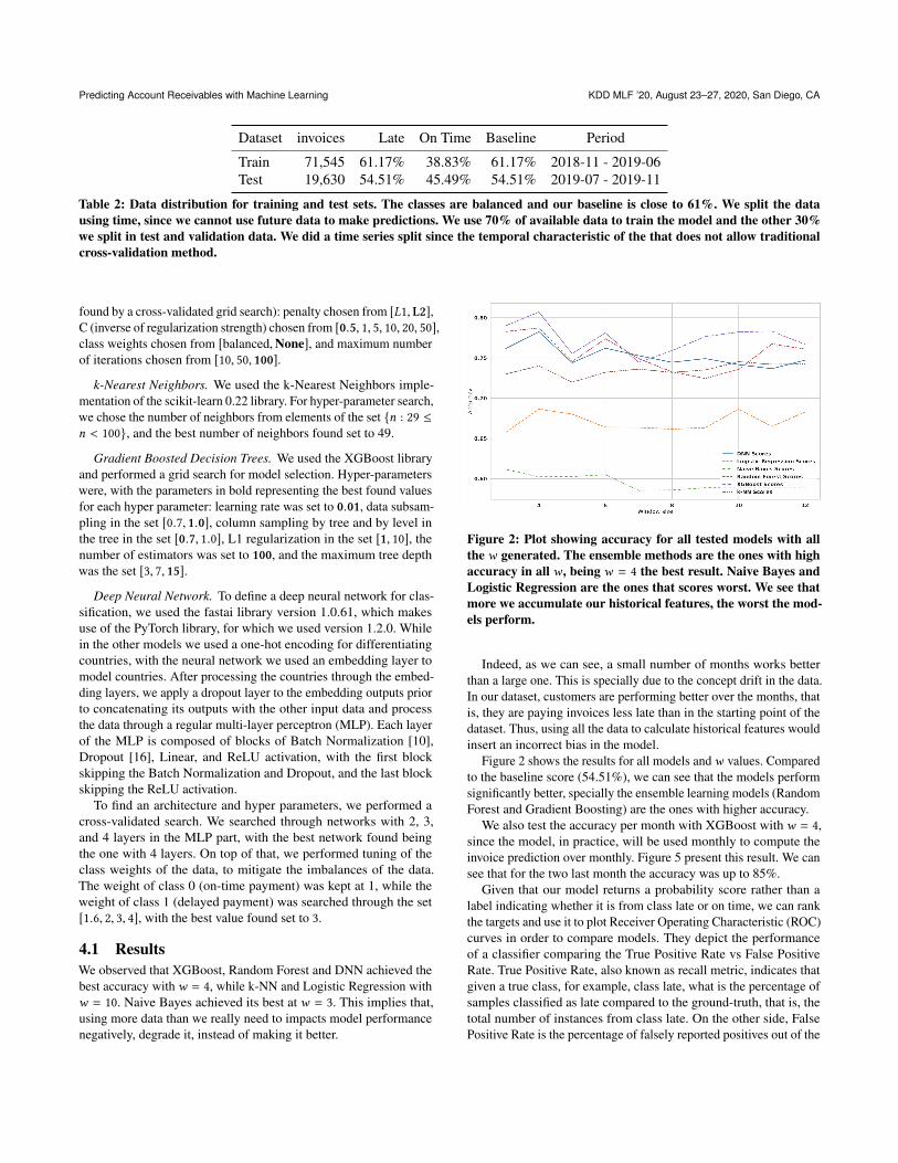
4.1 ResultsWe observed that XGBoost, Random Forest and DNN achieved thebest accuracy with w = 4, while k-NN and Logistic Regression withw = 10. Naive Bayes achieved its best at w = 3. This implies that,using more data than we really need to impacts model performancenegatively, degrade it, instead of making it better.

Figure 2: Plot showing accuracy for all tested models with allthe w generated. The ensemble methods are the ones with highaccuracy in all w , being w = 4 the best result. Naive Bayes andLogistic Regression are the ones that scores worst. We see thatmore we accumulate our historical features, the worst the mod-els perform.

Indeed, as we can see, a small number of months works betterthan a large one. This is specially due to the concept drift in the data.In our dataset, customers are performing better over the months, thatis, they are paying invoices less late than in the starting point of thedataset. Thus, using all the data to calculate historical features wouldinsert an incorrect bias in the model.

Figure 2 shows the results for all models andw values. Comparedto the baseline score (54.51%), we can see that the models performsignificantly better, specially the ensemble learning models (RandomForest and Gradient Boosting) are the ones with higher accuracy.

We also test the accuracy per month with XGBoost with w = 4,since the model, in practice, will be used monthly to compute theinvoice prediction over monthly. Figure 5 present this result. We cansee that for the two last month the accuracy was up to 85%.

Given that our model returns a probability score rather than alabel indicating whether it is from class late or on time, we can rankthe targets and use it to plot Receiver Operating Characteristic (ROC)curves in order to compare models. They depict the performanceof a classifier comparing the True Positive Rate vs False PositiveRate. True Positive Rate, also known as recall metric, indicates thatgiven a true class, for example, class late, what is the percentage ofsamples classified as late compared to the ground-truth, that is, thetotal number of instances from class late. On the other side, FalsePositive Rate is the percentage of falsely reported positives out of the


Figure 3: Accuracy per month in the test set with XGBoost andw = 4.

0.0 0.2 0.4 0.6 0.8 1.0False Positive Rate

0.2

0.4

0.6

0.8

1.0

True

Pos

itive

Rat

e

XGBoost AUC = 0.89Naive Bayes AUC = 0.75Logistic Regression AUC = 0.78k-NN AUC = 0.81Random Forest AUC = 0.87DNN AUC = 0.85

Figure 4: ROC Curve of all five methods we tested in our testdataset with w = 4.

ground-truth negatives (class on time). Intuitively, the ROC curveswill give a guidance to understand how well a model is performingbased on a ranking. That is, if we have a high lift point on the curve,it demonstrates that invoices with late labels have higher probabilityscore of being late (as expected).

In order to measure not only graphically but also quantitatively,we used the area under the curve metric (AUC) as well. AUC isa metric that calculates the area under our ROC curve, i.e., it as away of calculating the lift point explained above. Figure 4 shows theROC curves for each model and the corresponding AUC score fortest and validation.

Clearly, the best models are the Random Forest and GradientBoosting. Therefore, we developed the predictive invoices labelsystem based on an ensemble approach using both models.

With the model trained we finally can use if to help collectoroptimize AR processes. One way to do that is Figure 5, which could

Figure 5: Invoices to be received over one month, distributedover the payment data. Each point could have one or more in-voices.

Dataset NA Accuracy LA Accuracy General Accuracy

NA + LA 82.02 79.87 80.71NA 72.27 - 72.27LA - 78.91 78.91

Table 3: Model Accuracy using data from NA and LA togetherand separately. In the first line we show a model that wastrained with LA and NA data together and tested with eachregion individually (first two columns) and both together (thirdcolumn). NA (the second line) represents a model trained onlywith data in from the NA, and tested only with NA data. LA(third line) is the model trained only with data from LA andtested only data from LA. We can see that the accuracy is bet-ter using data from both LA and NA together.

be a interactive visualization showing the invoice distribution duedate over the month. Each day we have the invoices that are due fordata day label as late or on time. Each bubble could be link to a listof invoices (and clients) where the ones marked as late the collectorcould take a action. For instance, for the late invoices the collectorcould give a call remembering the payment. For each month when anew invoice is created the model will give a prediction if the invoicewill be payed Later or On Time, with this in hands, collectors canhave a better vision of the process and focus in clients that are predictto be late and only follow the invoices that are predict to be on timeto check if they were really payed. As we will show in the Section 5we also proposed a new way to prioritizing the clients that beforethe use of machine learning were sorted mainly by the amount ofmoney that they are in debt. Now, with the model we can use theprobability of an invoice be payed late to adjust this sort.

4.2 Model RobustnessAlthough the entirety of the dataset was created by same bank, thisdoesn’t mean the data is homogeneous. The bank has customers fromdifferent countries and each region uses different legacy systems,especially when we compare North America with Latin America.Therefore, it’s possible to have different behaviors from each countrydue to local economic factors and operational differences. Thesedifferences could have an impact in the model, showing the impor-tance to have a robust model that can learn this distinct patternsenabling the creation of a general model, capable of working withthe complete dataset and, consequently, with all the regions presentin the dataset.


In Table 3 we present an experiment with the XGBoost model andw = 4 to test the robustness of the model trained with the completedata contrasted with using only NA or LA data. The NA+LA lineshows a model that was trained with the full dataset, and showsthe evaluation performance of all the test set, and also for only theNA region, and only for the LA region. We can see that NA hasbetter accuracy on test, 82%. The other two models were trainedexclusively with NA and LA and tested only with data from theirrespective regions. We can see that the accuracy is lower usingseparate models both in LA and NA. Using both regions togetherwe were able to improve the accuracy and make the model morerobust. This also represents a benefit to the client, since the client isplanning on expanding to new geographies, and a single model iseasier to maintain than having several, separate ones.

5 INVOICE PRIORITIZATIONIn the previous section we demonstrated that we can effectivelypredict the probability of an invoice being late. Identifying invoicesthat are likely to be delinquent at the time of creation enables usto steer the collections process, thus helping to save resources [19].However, our objective is not to make decisions based on invoices.Rather, we intend to make decisions based on the clients that holdthe invoices. Furthermore, considering that resources are finite, wecan not work with the hypothesis that all invoices have the sameimpact. In other words, we have to associate the probability of aninvoice being late with its value in dollars. This way, we will be ableto measure the delinquency risk based not only on probabilities, butalso based on total invoice amount.

Currently, collectors can be considered agents that follow a greedypolicy based on the value of invoices. In other words, collectorswill prioritize invoices based on the total amount of dollars thatis overdue. As an example, consider the following hypotheticalsituation: suppose there is an invoice I1 with low probability ofbeing late, such as PI1 = 0.2506. But I1 has a high value, such asVI1 = $1, 000, 000.00. Suppose further that there exists an invoiceI2 that has a high probability of being late, PI2 = 0.9358, and alower value, such as VI2 = $300, 000.00. In this situation, withoutour model, I1 would have higher priority than I2.

As we show in Equation (2), we propose to take into account aninvoice’s risk of being late, multiplying its probability of being lateby its value. In this way, we can continue prioritizing big customersand, at the same time, we save efforts on customers which willprobably pay the invoice on time.

RIi = VIi ∗ PIi (Y = Late) (2)Next, we need to associate the invoice’s level of information with

a customer’s level of information. We assume that clients will becontacted based on their total amount of risk, rather than based solelyon a single invoice. To create a customer ranking, we decided toaverage the risk of invoices by customer as shown in Equation (3).

RCj =1N

N∑i=1

RIi (3)

In order to compare our new prioritization ranking with the previ-ous, greedy policy followed by collectors, we use Kendall’s τ [12] asa metric to compare the number of pairwise disagreements between

two orders. Values close to 1 indicate strong agreement, while val-ues close to -1 indicates strong disagreement. Our new ranking hasτ = −0.003 which means that we change about 50% of the rankingorder.

To investigate whether the ranking function proposed in this sec-tion can be effective in increasing recovery, we simulated how thesystem would behave when customers were contacted using thegreedy approach, and using the proposed ranking functions. To setup the simulation, we assumed collectors can contact a finite amountof customers per month. We performed the simulation consideringn = 100, 200, 300 calls. Since we don’t know the real impact a con-tact has on customers, we assigned a probability p of the contactbeing successful and resulting in the payment of an invoice. We var-ied p from 0 to 1 using a step size of 0.1. The probability of 0 servesas a sanity check for the simulation, since it means that calls have noeffect and, therefore, both rankings should result in the same amountof money collected. Although it is unrealistic that all customers willhave the same probability of reacting positively to a contact, thisis still a useful model to understand the overall impact of the newranking function.

Figure 6 shows the results of our simulation. In the figure, weshow the difference in savings (money collected) when using theproposed ranking compared to the greedy ranking function. Eachbox plot in the figure aggregates the data of a hundred independentsimulation runs. We performed the simulations for three differentmonths in our dataset. Each row of Figure 6 shows data for a par-ticular month, while each column shows the impact for a differentn, described above. The results show that, in every scenario, theranking function created with our model results in a better ranking,which increases the money collected up to approximately 1.75 mil-lion dollars. Smaller values of n show higher savings, which makessense: since collectors can’t contact many clients, the impact ofchoosing which clients to contact becomes more important. This isin line with reality, since collectors have a limitation in the numberof clients that they are able to call in a month.

As can be seen in the figure, the bigger p gets, the bigger arethe savings. This happens because, as the probability increases, theimpact of correct prioritization becomes more apparent, since abetter ranking might be able to change invoices that would becomeoverdue into invoices that become paid on time. Impact is higheron the first month because we have more data for that month. Ourdataset comprises 7089, 4260 and 2626 entries for months 1, 2 and3 respectively.

6 CONCLUSIONIn this paper, we built a model that computes the probability scoreof an invoice being overdue in the context of AR practices. Thisis critical when dealing with a very large set of invoices, which inturn requires collectors to rank customers and focus on those morelikely to be delinquent. Our results are significant, with an accuracyof up to 81%. The model developed in our work will be able to helpour client attain a better sense of its AR operations and take betteractions, thus improving its cash flow.

Our set of historical features is small and captures the customerbehavior payment using temporal information to make better predic-tion. We demonstrated by our experiments that using the window


Figure 6: Simulation of the probability of a invoice being payed given a call from collector. The n represents the number of clientsthat a collector will call 100, 200, 300. We also vary the probability of payment given a call on axis x and the savings in millions of USDin axis y compared with traditional ranking.

size with a small number of months (4) we were able to deal withconcept drift in the dataset. We also created a new prioritization listthat is able to rank customers in a more realistic way, helping theclient to optimize their resources with respect to daily action of thecollectors.

As real world environments are always in continuous flux, ourfeatures distribution are shifting as well. We noted that the currentAR process has been modified over the last year, and, as it evolves,our model should accompany that. We thus recommend a continuous

evaluation of the analytics results so as to keep track of accuracymetrics as well as AUC, as discussed in the results section. From timeto time, it seems necessary to retrain the model since all processessuffer from what is called concept drift, i.e., the relationship betweenthe features and the labels evolve over time and classical machinelearning approaches consider only stationary data.

Finally, we validated our proposed ranking function with a simu-lation that shows savings up to ≈1.75 million dollars, suggesting theproposed approach will have positive impact in the real world.


REFERENCES[1] Naoki Abe, Prem Melville, Cezar Pendus, Chandan K Reddy, David L Jensen,

Vince P Thomas, James J Bennett, Gary F Anderson, Brent R Cooley, MelissaKowalczyk, et al. 2010. Optimizing debt collections using constrained reinforce-ment learning. In Proceedings of the 16th ACM SIGKDD international conferenceon Knowledge discovery and data mining. ACM, 75–84.

[2] Bart Baesens, Tony Van Gestel, Maria Stepanova, Dirk Van den Poel, and JanVanthienen. 2005. Neural network survival analysis for personal loan data. Journalof the Operational Research Society 56, 9 (2005), 1089–1098.

[3] DR Bailey, B Butler, T Smith, T Swift, J Williamson, and WT Scherer. 1999.Providian Financial Corporation: Collections Strategy. In Systems EngineeringCapstone Conference. University of Virginia.

[4] Leo Breiman. 2001. Random Forests. Mach. Learn. 45, 1 (Oct. 2001), 5–32.https://doi.org/10.1023/A:1010933404324

[5] Ricardo Cao, Juan M Vilar, and Andrés Devia. 2009. Modelling consumer creditrisk via survival analysis. SORT: statistics and operations research transactions33, 1 (2009), 0003–30.

[6] Michelle LF Cheong and Wen SHI. 2018. Customer level predictive modeling foraccounts receivable to reduce intervention actions. (2018).

[7] Lore Dirick, Gerda Claeskens, and Bart Baesens. 2017. Time to default in creditscoring using survival analysis: a benchmark study. Journal of the OperationalResearch Society 68, 6 (01 Jun 2017), 652–665. https://doi.org/10.1057/s41274-016-0128-9

[8] Jerome H. Friedman. 2002. Stochastic gradient boosting. Computational Statistics& Data Analysis 38, 4 (2002), 367 – 378. https://doi.org/10.1016/S0167-9473(01)00065-2 Nonlinear Methods and Data Mining.

[9] Jeremy Howard and Sylvain Gugger. 2020. Fastai: A Layered API for Deep Learn-ing. Information 11, 2 (Feb 2020), 108. https://doi.org/10.3390/info11020108

[10] Sergey Ioffe and Christian Szegedy. 2015. Batch normalization: Accelerat-ing deep network training by reducing internal covariate shift. arXiv preprintarXiv:1502.03167 (2015).

[11] Gareth James, Daniela Witten, Trevor Hastie, and Robert Tibshirani. 2014. AnIntroduction to Statistical Learning: With Applications in R. Springer PublishingCompany, Incorporated.

[12] Maurice George Kendall. 1948. Rank correlation methods. (1948).[13] Elisa T. Lee and John Wenyu Wang. 2013. Statistical Methods for Survival Data

Analysis (4th ed.). Wiley Publishing.[14] Michal Rychnovsky et al. 2018. Survival Analysis as a Tool for Better Probability

of Default Prediction. Acta Oeconomica Pragensia 2018, 1 (2018), 34–46.[15] Janika Smirnov et al. 2016. Modelling late invoice payment times using survival

analysis and random forests techniques. Ph.D. Dissertation.[16] Nitish Srivastava, Geoffrey Hinton, Alex Krizhevsky, Ilya Sutskever, and Ruslan

Salakhutdinov. 2014. Dropout: a simple way to prevent neural networks fromoverfitting. The journal of machine learning research 15, 1 (2014), 1929–1958.

[17] Tarun Tater, Sampath Dechu, Senthil Mani, and Chandresh Maurya. 2018. Predic-tion of Invoice Payment Status in Account Payable Business Process. In Interna-tional Conference on Service-Oriented Computing. Springer, 165–180.

[18] Bashar Younes. 2013. A Framework for Invoice Management in Construction.Ph.D. Dissertation. University of Alberta.

[19] Sai Zeng, Prem Melville, Christian A Lang, Ioana Boier-Martin, and ConradMurphy. 2008. Using predictive analysis to improve invoice-to-cash collection. InProceedings of the 14th ACM SIGKDD international conference on Knowledgediscovery and data mining. ACM, 1043–1050.

https://doi.org/10.1023/A:1010933404324

https://doi.org/10.1057/s41274-016-0128-9

https://doi.org/10.1057/s41274-016-0128-9

https://doi.org/10.1016/S0167-9473(01)00065-2

https://doi.org/10.1016/S0167-9473(01)00065-2

https://doi.org/10.3390/info11020108

Documents

Predicting Account Receivables with Machine Learning