Embed Size (px)
Citation preview

Linkoping Studies in Science and Technology
Thesis No. 1503
Predictable Real-Time Applications onMultiprocessor Systems-on-Chip
by
Jakob Rosen
Submitted to Linkoping Institute of Technology at Linkoping University in partialfulfilment of the requirements for degree of Licentiate of Engineering
Department of Computer and Information ScienceLinkoping University
SE–581 83 Linkoping, Sweden
Linkoping 2011

This is a Swedish Licentiate’s Thesis.The Licentiate’s degree comprises 120 ECTS credits of postgraduate
studies.
ISBN 978-91-7393-090-1, ISSN 0280-7971Printed by LiU-Tryck, Linkoping, Sweden 2011Copyright c© 2011 Jakob RosenElectronic version:http://urn.kb.se/resolve?urn=urn:nbn:se:liu:diva-70138

PRESS PLAY ON TAPE


Predictable Real-Time Applications onMultiprocessor Systems-on-Chip
by
Jakob Rosen
September 2011ISBN 978-91-7393-090-1
Linkoping Studies in Science and TechnologyThesis No. 1503ISSN 0280-7971
LIU-TEK-LIC-2011:42
ABSTRACT
Being predictable with respect to time is, by definition, a fundamental require-ment for any real-time system. Modern multiprocessor systems impose a challengein this context, due to resource sharing conflicts causing memory transfers to becomeunpredictable. In this thesis, we present a framework for achieving predictability forreal-time applications running on multiprocessor system-on-chip platforms. Usinga TDMA bus, worst-case execution time analysis and scheduling are done simul-taneously. Since the worst-case execution times are directly dependent on the busschedule, bus access design is of special importance. Therefore, we provide an ef-ficient algorithm for generating bus schedules, resulting in a minimized worst-caseglobal delay.
We also present a new approach considering the average-case execution time ina predictable context. Optimization techniques for improving the average-case ex-ecution time of tasks, for which predictability with respect to time is not required,have been investigated for a long time in many different contexts. However, this hastraditionally been done without paying attention to the worst-case execution time.For predictable real-time applications, on the other hand, the focus has been solelyon worst-case execution time optimization, ignoring how this affects the executiontime in the average case. In this thesis, we show that having a good average-caseglobal delay can be important also for real-time applications, for which predictabil-ity is required. Furthermore, for real-time applications running on multiprocessorsystems-on-chip, we present a technique for optimizing for the average case and theworst case simultaneously, allowing for a good average case execution time while stillkeeping the worst case as small as possible. The proposed solutions in this thesishave been validated by extensive experiments. The results demonstrate the efficiencyand importance of the presented techniques.
This research work was funded in part by CUGS (the National Graduate School ofComputer Science, Sweden).
Department of Computer and Information ScienceLinkopings universitet
SE–581 83 Linkoping, Sweden


Acknowledgments
So, here I am. The end of this winding road has been reached, and thethesis is finally ready. However, I would never have come to this pointwithout the many people who gave me support, inspiration and courageduring the past years. Let me first start by thanking my supervisorsZebo Peng and Petru Eles, for giving me the opportunity to become agraduate student and for always believing in me. I am very grateful forthat. The working environment at IDA has been excellent, and I wishI could thank every one of my colleagues individually. If you work hereand read this, consider yourself thanked!
Carl-Fredrik Neikter did a fantastic job contributing to the frame-work which this thesis is built upon, and I truly enjoyed our collab-oration. Alexandru Andrei spent many late nights helping me withtechnical issues during the writing of our first paper, and for that Iam thankful. I also want to thank Soheil Samii and Sergiu Rafiliu forour frequent and (usually) very enjoyable “board meetings”, where wediscussed all kinds of subjects related to our work.
Anton Blad and Fredrik Kuivinen have been my friends for a longtime, and I really enjoyed the luxury of also having them as colleaguesfor a while. In particular, I want to thank them for the fun momentswe spent developing the TRUT64 device (and testing it!), and of coursealso for just being such great guys. Furthermore, I want to expressgratitude to Traian Pop for introducing me to the world of research ina friendly manner, and for throwing the best birthday parties. A bigthank you must also go to everyone who participated in the official duckfeeding sessions at the university pond, and to the geese and the ducksfor kindly accepting the bread that I brought.
Finally, I thank my family for giving me love and support. Always.
Jakob Rosen
Linkoping, August 2011
iii


Contents
1 Introduction 1
1.1 Multiprocessor Real-Time Systems . . . . . . . . . . . . 2
1.2 Related Work . . . . . . . . . . . . . . . . . . . . . . . . 3
1.3 Contribution . . . . . . . . . . . . . . . . . . . . . . . . 5
1.4 Thesis Organization . . . . . . . . . . . . . . . . . . . . 5
2 System Model 7
2.1 Hardware Architecture . . . . . . . . . . . . . . . . . . . 7
2.2 Application Model . . . . . . . . . . . . . . . . . . . . . 8
2.3 Bus Model . . . . . . . . . . . . . . . . . . . . . . . . . . 9
3 Predictability Approach 13
3.1 Motivational Example . . . . . . . . . . . . . . . . . . . 13
3.2 Overall Approach . . . . . . . . . . . . . . . . . . . . . . 15
4 Worst-Case Execution Time Analysis 19
4.1 TDMA-Based WCET Analysis . . . . . . . . . . . . . . 19
4.2 Compositional WCET Analysis Flow . . . . . . . . . . . 20
v

vi Contents
4.2.1 Monoprocessor WCET Example . . . . . . . . . 214.2.2 Multiprocessor WCET Example . . . . . . . . . 23
4.3 Noncompositional Analysis . . . . . . . . . . . . . . . . 25
5 Bus Schedule Optimization 275.1 WCGD Optimization . . . . . . . . . . . . . . . . . . . . 275.2 Cost Function . . . . . . . . . . . . . . . . . . . . . . . . 285.3 Optimization Approach . . . . . . . . . . . . . . . . . . 30
5.3.1 Slot Order Selection . . . . . . . . . . . . . . . . 305.3.2 Determination of Initial Slot Sizes . . . . . . . . 315.3.3 Generation of New Slot Size Candidates . . . . . 345.3.4 Density Regions . . . . . . . . . . . . . . . . . . 35
5.4 Simplified Algorithm . . . . . . . . . . . . . . . . . . . . 385.5 Memory Consumption . . . . . . . . . . . . . . . . . . . 395.6 Experimental Results . . . . . . . . . . . . . . . . . . . . 40
5.6.1 Bus Schedule Approaches . . . . . . . . . . . . . 415.6.2 Synthetic Benchmarks . . . . . . . . . . . . . . . 435.6.3 Real-Life Example . . . . . . . . . . . . . . . . . 45
6 Worst/Average-Case Optimization 496.1 Motivation . . . . . . . . . . . . . . . . . . . . . . . . . 506.2 Average-Case Execution Time Estimation . . . . . . . . 526.3 Combined Optimization Approach . . . . . . . . . . . . 576.4 Bus Access Optimization for ACGD and WCGD . . . . 58
6.4.1 Task and Bus Segments . . . . . . . . . . . . . . 596.4.2 Bus Bandwidth Distribution Analysis . . . . . . 616.4.3 Cost Function . . . . . . . . . . . . . . . . . . . . 636.4.4 Bus Schedule Optimization . . . . . . . . . . . . 64
6.5 Experimental Results . . . . . . . . . . . . . . . . . . . . 65
7 Conclusions 69
A Bus Bandwidth Calculations 77A.1 Bus Bandwidth Calculations . . . . . . . . . . . . . . . 77
A.1.1 Calculation of the Desired Bus Bandwidth . . . . 77A.1.2 Calculation of the Current Bus Bandwidth . . . 80

List of Figures
2.1 Hardware Model . . . . . . . . . . . . . . . . . . . . . . 8
2.2 Task graph . . . . . . . . . . . . . . . . . . . . . . . . . 9
2.3 Example of a bus schedule . . . . . . . . . . . . . . . . . 10
2.4 Bus schedule table representation . . . . . . . . . . . . . 11
3.1 Motivational example . . . . . . . . . . . . . . . . . . . 14
3.2 Overall approach example . . . . . . . . . . . . . . . . . 16
3.3 Overall approach . . . . . . . . . . . . . . . . . . . . . . 18
4.1 WCET tool program flow . . . . . . . . . . . . . . . . . 21
4.2 Example CFG . . . . . . . . . . . . . . . . . . . . . . . . 22
4.3 Example TDMA bus schedule . . . . . . . . . . . . . . . 23
5.1 Estimating the global delay . . . . . . . . . . . . . . . . 29
5.2 The optimization approach . . . . . . . . . . . . . . . . 30
5.3 Close-up of two tasks . . . . . . . . . . . . . . . . . . . . 32
5.4 Calculation of new slot sizes . . . . . . . . . . . . . . . . 34
5.5 Subtask evaluation algorithm . . . . . . . . . . . . . . . 39
vii

viii LIST OF FIGURES
5.6 The simplified optimization approach . . . . . . . . . . . 405.7 BSA1 bus schedule . . . . . . . . . . . . . . . . . . . . . 415.8 BSA2 bus schedule . . . . . . . . . . . . . . . . . . . . . 425.9 BSA3 bus schedule . . . . . . . . . . . . . . . . . . . . . 425.10 BSA4 bus schedule . . . . . . . . . . . . . . . . . . . . . 435.11 Four bus access policies . . . . . . . . . . . . . . . . . . 445.12 Comparison between BSA2 and BSA3 . . . . . . . . . . 465.13 BSA2 optimization steps . . . . . . . . . . . . . . . . . . 46
6.1 Motivational example for a hard real-time system . . . . 516.2 Motivational example for a buffer-based system . . . . . 516.3 Example histogram for 1000 executions . . . . . . . . . 536.4 Example histogram for 12 executions . . . . . . . . . . . 536.5 Example table for hypothetical path classification . . . . 546.6 Example table for cache miss selection . . . . . . . . . . 556.7 Three hypothetical execution paths and the correspond-
ing average-case execution time estimation . . . . . . . . 576.8 Combined optimization approach . . . . . . . . . . . . . 586.9 Example task graph . . . . . . . . . . . . . . . . . . . . 606.10 Average-case chart . . . . . . . . . . . . . . . . . . . . . 606.11 Average-case chart with corresponding execution paths . 616.12 Average-case chart with density regions . . . . . . . . . 616.13 The improve function . . . . . . . . . . . . . . . . . . . 666.14 Relative ACGD improvement . . . . . . . . . . . . . . . 676.15 Relative ACGD improvement and WCGD extension . . 68

Abbreviations
ACET Average-Case Execution TimeACGD Average-Case Global DelayBSA Bus Scheduling ApproachCFG Control Flow GraphDS Density Region Based SizesISS Initial Slot SizesNWCET Naive Worst-Case Execution TimeQoS Quality of ServiceSSA Slot Size AdjustmentsTDMA Time Division Multiple AccessWCET Worst-Case Execution TimeWCGD Worst-Case Global Delay
ix

x Abbreviations

1
Introduction
Embedded real-time systems have become a key part of our society,helping us in almost every aspect of our daily living. Of significantimportance is the class of safety-critical embedded real-time systems, towhich we entrust our lives, for instance at hospitals, in aeroplanes and incars. These systems must be reliable and, consequently, it is of crucialimportance that they are predictable with respect to time. However,predictability is desirable not only for this kind of traditional hard real-time systems, but for any system exhibiting real-time properties.
This thesis describes techniques for designing predictable embeddedreal-time systems in a multiprocessor environment. Besides serving asan introduction to the topic, this chapter presents a summary of thestate-of-the-art research within the field. After briefly describing thecontributions of this thesis, the chapter ends with an outline of whatfollows next.
1

2 CHAPTER 1. INTRODUCTION
1.1 Multiprocessor Real-Time Systems
For real-time systems, correctness of a program not only depends onthe produced computational results, but also on its ability to deliverthese on time, according to specified time constraints. Therefore, for areal-time application, predictability with respect to time is of uttermostimportance. The obvious example is safety-critical hard real-time sys-tems, such as medical and avionic applications, for which failure to meeta specified deadline not only renders the computations useless, but alsocan have catastrophic consequences. However, predictability is gettingmore and more desirable also for other classes of embedded applications,for instance within the domains of multimedia and telecommunication,for which QoS guarantees are desired [8].
As these kinds of applications become increasingly complex, theyalso require more computational power in terms of hardware resources.Generally, the trend in processor design is to increase the number ofcores as means to improve the performance and power efficiency, andmicroprocessors with hundreds of cores are expected to arrive on themarket in the not-so-distant future [4]. In order to satisfy the demandsof complex and resource-demanding embedded systems, for which pre-dictability is required, multicore systems implemented on a single chipare used to an increasing extent [16, 36].
To achieve predictability with respect to time, schedulability analy-sis techniques are applied, assuming that the worst-case execution time(WCET) of every task is known. A lot of research has been carried outwithin the area of worst-case execution time analysis [21]. However,according to the proposed techniques, each task is analyzed in isola-tion, as if it was running on a monoprocessor system. Consequently, itis assumed that memory accesses over the bus take a constant amountof time to process, since no bus conflicts can occur. For multipro-cessor systems with a shared communication infrastructure, however,transfer times depend on the bus load and are therefore no longer con-stant, causing the traditional methods to produce incorrect results [32].The main obstacle when performing timing analysis on multiprocessorsystems is that the scheduling of tasks assumes that their worst-caseexecution times are known, but to calculate these worst-case executiontimes, knowledge about the task schedule is required. Clearly, the tra-ditional method of separating WCET analysis and task scheduling nolonger works, and new approaches are required.
Of great interest when measuring the execution time of a real-time

1.2. RELATED WORK 3
application is the global delay, defined as the time it takes to executethe application from its beginning to the very end. In this thesis, wepropose an approach for designing predictable real-time embedded sys-tems on multiprocessor system-on-chip architectures. We show how it ispossible to design predictable systems using a TDMA bus architecture,and we also propose algorithms for generating intelligent bus schedulesminimizing the worst-case global delay (WCGD) of the application.
Furthermore, we take a new approach to hard real-time system de-sign by, in addition, also considering the effects on the average-caseglobal delay (ACGD) while making sure that the WCGD is kept to anear-minimum. Optimization techniques for improving the average caseexecution time of an application, for which predictability with respectto time is not required, have been investigated in nearly every scientificdiscipline involving a computer. However, this has traditionally beendone without paying attention to the worst-case execution time. Forpredictable applications, on the other hand, the focus has been solelyon worst-case execution time optimization, which still is a hot researchtopic [6, 7]. To the best of our knowledge, this is the first time the com-bination of these two concepts has been investigated within the contextof achieving predictability.
1.2 Related Work
The fundament for achieving predictability is worst-case execution time(WCET) analysis, and a lot of research has been carried out within thisarea. Wilhelm et al. present an overview of the existing methods andtools [33]. None of them can, however, be applied directly to mul-tiprocessor systems with a shared communication infrastructure, sincethese techniques assume a monoprocessor environment. Yan and Zhangpresent a new approach for worst-case execution time analysis on mul-ticore processors with shared L2 caches [37]. They describe their workas a first, important step towards a complete framework rather than afull solution to the problem.
One approach is to use an additive bus model, assuming that con-flicts on the bus do not affect the calculated worst-case execution timessignificantly compared to when running the same program on a mono-processor platform. It has been shown that this is a good assumptionif the bus load is kept below 60% [2], but even for such low bus loads,no worst-case execution time guarantees can be made. Furthermore,

4 CHAPTER 1. INTRODUCTION
increasing the number of processor cores will also increase the bus con-gestion [35] and, thus, the additive bus model is likely to not performwell for future architectures, even when strict time-predictability is notrequired.
Schoeber and Puschner present a technique for achieving predictabil-ity on TDMA bus-based chip multiprocessors [30]. Similar to the ap-proach in this thesis, the output from the worst-case execution timeanalysis is used to improve the bus schedule. However, in order toavoid the problem of scheduling tasks, they assume that the number ofcores are greater than the number of tasks.
In a recently published paper, Lv et al. use abstract modeling inUppaal to calculate the worst-case execution time of tasks runningon multiprocessor systems with a shared communication infrastructure[14]. The contribution of their approach is a very general frameworkwith support for many kinds of buses. However, their solution does nothandle computer architectures exhibiting timing anomalies.
Within the context of response time analysis [9], Schliecker et al.propose a technique using accumulated busy times instead of consid-ering each memory access individually [29]. The result is a frameworkfor multiprocessor analysis that computes worst-case response timeswith good precision, but without providing any hard timing guaran-tees. A more recent approach by the same authors provides conser-vative bounds, but without support for noncompositional architectures[28]. Schranzhofer et al. present a technique for response time analy-sis for TDMA bus-based multiprocessor systems with shared resources[31]. The analysis is safe, but does not support the presence of timinganomalies. Pellizzoni and Caccamo propose an approach for calculatingthe delay caused by bus interference for tasks running on systems withseveral connected peripherals [19]. They also provide a correspondingschedulability analysis framework.
Edwards and Lee argue in favor of hardware customized for achievingtiming predictability, in contrast to today’s platforms optimized solelyfor good average case performance [5]. Lickly et al. present an exam-ple of one such processor [12]. However, no such hardware exists on themarket today. Paolieri et al. propose a predictable multiprocessor hard-ware architecture, using custom bus arbiters, designed for running hardand soft real-time tasks concurrently [17]. For hard real-time tasks, itprovides a maximum bound on the memory access transfer time. Thebig advantage of this approach is that traditional worst-case execution

1.3. CONTRIBUTION 5
time analysis techniques can be used without modifications. However,applications with many hard real-time tasks will make this upper boundbecome large, potentially increasing the pessimism.
1.3 Contribution
The main contributions of this thesis are:
1. We propose a novel technique to achieve predictability on mul-tiprocessor systems by doing worst-case execution time analysisand scheduling simultaneously [1, 23, 24]. With respect to a givenTDMA bus schedule, tasks are scheduled at the same time as theirworst-case execution times are calculated, and the resulting worst-case global delay of the application is obtained.
2. To generate good bus schedules, we have constructed efficient op-timization algorithms that minimize the worst-case global delayof the given application [23].
3. Combining optimization for the worst case and the average case,we have developed an approach to achieve a good average-caseglobal delay while still keeping the worst-case delay as small aspossible [25].
1.4 Thesis Organization
The remaining part of the thesis is outlined as follows. In the nextchapter, the system model is described in detail. The overall approachfor achieving predictability is then presented in Chapter 3. In Chapter4, we discuss the underlying worst-case analysis framework necessaryfor implementing our approach. Chapter 5 presents algorithms for op-timization of the worst-case global delay using several bus schedulingapproaches. Experimental results are presented at the end of the chap-ter. The algorithms for combining WCGD and ACGD optimization arepresented in Chapter 6, together with a motivation for why the averagecase is important also for predictable real-time systems. The chapterends with experimental results validating our approach. Finally, Chap-ter 7 presents our conclusions.

6 CHAPTER 1. INTRODUCTION

2
System Model
This chapter starts by describing the hardware platform that is assumedthroughout the rest of the thesis. Next, the software application modelis explained. Finally, we describe the model of the TDMA-based com-munication infrastructure.
2.1 Hardware Architecture
As hardware platform, we have considered a multiprocessor system-on-chip architecture with a shared communication infrastructure, as shownin Figure 2.1, typical for the new generation of multiprocessor system-on-chip designs [11]. Each processor has its own cache for storing dataand instructions, and is connected to a private memory via the bus. Forinterprocessor communication, a shared memory is used. All memoryaccesses to the private memories are cached, as opposed to accesses tothe shared memory which, in order to avoid cache coherence problems,are not cached. All memory devices are accessed using the same, sharedbus. However, in the case of private memory accesses, the bus is usedonly when an access results in a cache miss.
7

8 CHAPTER 2. SYSTEM MODEL
Bus
CPU 1
Cache
CPU 2
Cache
Memory 1(Private)
Memory 0(Shared)
Memory 2(Private)
Figure 2.1 Hardware Model
Within the context of worst-case execution time analysis, hardwareplatforms can be divided into compositional architectures and noncom-positional architectures [34], depending on whether or not the platformexhibits timing anomalies [13, 22]. Timing anomalies occur when alocal worst-case scenario, such as a cache miss instead of a hit, doesnot result in the worst case globally. This complicates the worst-caseexecution time analysis significantly, since no local assumptions canbe made. Compositional architectures, such as the ARM7, do not ex-hibit timing anomalies, and the analysis can therefore be divided intodisjunct subproblems, simplifying the analysis procedure. Noncomposi-tional architectures, on the other hand, require a far more complicatedand time-consuming analysis. The PowerPC 775 is an example of anoncompositional architecture [34]. As will be described further on,our approach works for both compositional architectures and noncom-positional architectures.
2.2 Application Model
The functionality of a software application is captured by a directedacyclic task graph, G(Π,Γ). Its nodes Π represent computational tasks,and the edges Γ represent data dependencies between them. A taskcannot start executing before all of its input data is available. Com-munication between tasks mapped on the same processor is performedby using the corresponding private memory, and is handled in the sameway as other memory requests during the execution of a task. Inter-processor communication, or so called explicit communication, is donevia the shared memory and is modeled as two communication tasks –one for transmitting and one for receiving – in the task graph. Thetransmitting communication task is assigned to the same processor as
2.3. BUS MODEL 9
τ1
τ2
τ1
τ1w
τ2r
τ3 dl=4 ms
Mapped on processor 1Mapped on processor 2
Figure 2.2 Task graph
the task that is sending data to the shared memory, and similarly thereceiving communication task is assigned to the processor fetching thesame data. An example is shown in Figure 2.2 where τ1w and τ2r rep-resent the transmitting and receiving task, respectively.
A computational task cannot communicate with other tasks duringits execution, which means that it will not access the shared memory.However, the task is accessing data, used in the computations, fromits private memory and program instructions are continuously fetched.Consequently, the bus is accessed every time a cache miss occurs, re-sulting in what we define as implicit communication. As opposed to ex-plicit communication, implicit communication has not been taken intoaccount in previous approaches for real-time application system-levelscheduling and optimization [20, 27].
The task graph has a deadline which represents the maximum al-lowed execution time of the entire application, known as the maximumglobal delay. Individual tasks can have deadlines as well. The exampletask graph in Figure 2.2 has a global delay of 4 milliseconds. The ap-plication is assumed to be running periodically, with a period greaterthan or equal to the application deadline.
2.3 Bus Model
A precondition for achieving predictability is to use a predictable busarchitecture. Therefore, we are using a TDMA-based bus arbitrationpolicy, which is suitable for modern system-on-chip designs with QoS

10 CHAPTER 2. SYSTEM MODEL
Slot belonging to CPU 1 Slot belonging to CPU 2
Segment 1 (ω1) Segment 2 (ω
2)
Round 1 Round 2
0 10 30 40 60 70 80 90 100 110 120
Figure 2.3 Example of a bus schedule
constraints [8, 18, 26].The behavior of the bus arbiter is defined by the bus schedule, con-
sisting of sequences of slots representing intervals of time. Each slot isowned by exactly one processor, and has an associated start time andan end time. Between these two time instants, only the processor own-ing the slot is allowed to use the bus. A bus schedule is divided intosegments, and each segment consists of a round, that is, a sequence ofslots that is repeated periodically. See Figure 2.3 for an example.
The bus arbiter stores the bus schedule in a dedicated external mem-ory, and grants access to the processors accordingly. If processor CPUi
requests access to the bus in a time interval belonging to a slot ownedby a different processor, the transfer will be delayed until the start ofthe next slot owned by CPUi. A bus schedule is defined for one periodof the application, and is then repeated periodically. A table represen-tation of the bus schedule in Figure 2.3 can be found in Figure 2.4.
To limit the required amount of memory on the bus controller neededto store the bus schedule, a TDMA round can be subject to variouscomplexity constraints. A common restriction is to let every processorown, at most, a specified number of slots per round. Also, one can letthe sizes be the same for all slots of a certain round, or let the slot orderbe fixed.

2.3. BUS MODEL 11
Segment start
Segment length
0
60
Processor ID 1
Slot size 10
Processor ID 2
Slot size 20
Segment 1
Round 1
Segment start
Segment length
60
120
Processor ID 1
Slot size 10
Processor ID 2
Slot size 10
Segment 2
Round 2
Figure 2.4 Bus schedule table representation

12 CHAPTER 2. SYSTEM MODEL

3
Predictability Approach
This chapter begins with a motivational example illustrating the prob-lems encountered when designing predictable multiprocessor-based real-time systems. It then continues by describing our overall approach toachieve predictability for such systems.
3.1 Motivational Example
Consider two tasks running on a multiprocessor system with two proces-sors and a shared communication infrastructure according to Chapter 2.Each task has been analyzed with a traditional WCET tool, assuming amonoprocessor system, and the resulting Gantt chart of the worst-casescenario is illustrated in Figure 3.1a. The dashed intervals representcache misses, each of them taking six time units to serve, and the whitesolid areas represent segments of code not using the bus. The task run-ning on processor 2 is also, at the end of its execution, transferring datato the shared memory, and this is represented by the black solid area.
However, since the tasks are actually running on a multiprocessorsystem with a shared communication infrastructure, they do not have
13

14 CHAPTER 3. PREDICTABILITY APPROACH
CPU1
CPU2
6 9 15 33 39 57
dl=63
6 11 17 24 36
CPU1
CPU2
BUS
6 9 18 36 49 67
dl=63
12 17 24 31 43
1 2 1 2 2 1
Deadlineviolation!
CPU1
CPU2
BUS 2
6 9 15 33 39 57
dl=63
21 26
1 1 2
32 39 51
2 1
CPU1 CPU2 CPU1 CPU2
6 12 18 24 31 4943
a) Two Concurrent Tasks
b) FCFS Arbitration
c) TDMA Arbitration
Figure 3.1 Motivational example
exclusive access to the bus handling the communication with the mem-ories. Hence, some kind of arbitration policy must be applied to dis-tribute the bus bandwidth among the tasks. The result is that whentwo tasks request the bus simultaneously, one of them has to wait untilthe other has finished transferring. This means that transfer times areno longer constant. Instead, they now depend on the bus conflicts re-sulting from the execution load on the different processors. Figure 3.1bshows the corresponding Gantt chart when the commonly used FCFSarbitration policy is applied.
The fundamental problem when performing worst-case executiontime analysis on multiprocessor systems is that the load on the otherprocessors is in general not known. For a task, the number of cache
3.2. OVERALL APPROACH 15
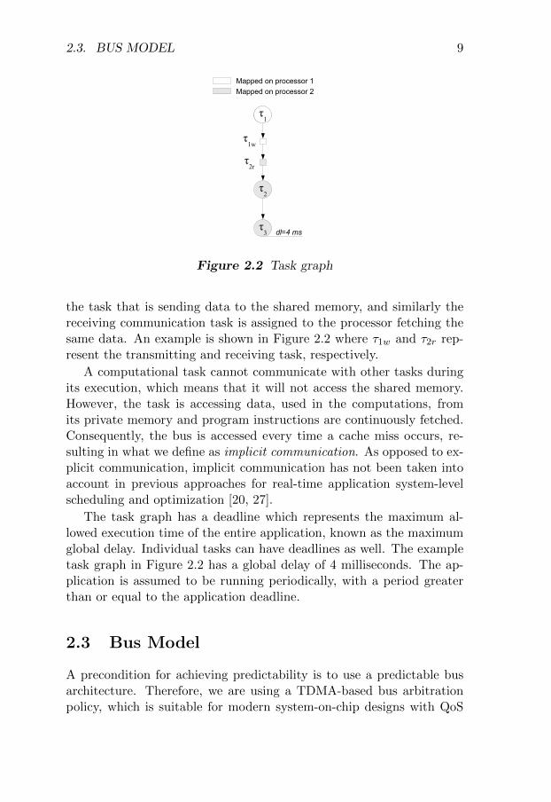
misses and their location in time depend on the program control flowpath. This means that it is very hard to foresee where there will bebus access collisions, since this will differ from execution to execution.To complicate things further, the worst-case control flow path of thetask will change depending on the bus load originating from the otherconcurrent tasks. In order to solve this and introduce predictability, weuse a TDMA bus schedule which, a priori, determines exactly when aprocessor is granted the bus, regardless of what is executed on the otherprocessors. Given a TDMA bus schedule, the WCET analysis tool cal-culates a corresponding worst-case execution time. Some bus scheduleswill result in relatively short worst-case execution times, whereas otherswill be very bad for the worst case. Therefore, it is important that aclever bus schedule, optimized to reduce the worst case, is used. Algo-rithms for this will be presented in Chapter 5. Note that regardless ofwhat bus schedule is given as input to the WCET analysis algorithm,the corresponding worst-case execution time will always be safe. Fig-ure 3.1c shows the same task configuration as previously, but now thememory accesses are arbitrated according to a TDMA bus schedule.
3.2 Overall Approach
For a task running on a multiprocessor system, as described in Chapter2, the problem for achieving predictability is that the duration of a bustransfer depends on the bus congestion. Since bus conflicts depend onthe task schedule, WCET analysis cannot be performed before that isknown. However, task scheduling traditionally assumes that the worst-case execution times of the tasks to be scheduled are already calculated.
To solve this circular dependency, we have developed an approachbased on the following principles:
1. A TDMA-based bus access policy, according to Section 2.3, isused for arbitration. The bus schedule, created at design time, isenforced during the execution of the application.
2. The worst-case execution time analysis is performed with respectto the bus schedule, and is integrated with the task schedulingprocess, as described in Figure 3.3.
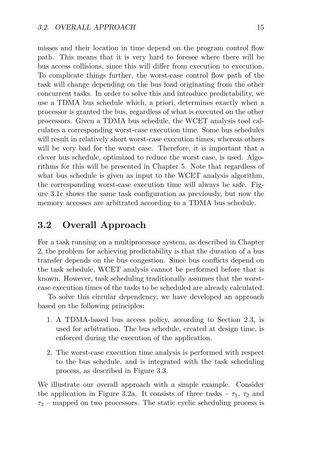
We illustrate our overall approach with a simple example. Considerthe application in Figure 3.2a. It consists of three tasks – τ1, τ2 andτ3 – mapped on two processors. The static cyclic scheduling process is

16 CHAPTER 3. PREDICTABILITY APPROACH
τ1
τ2
τ3
CPU1
CPU2
τ1
τ2
a) Task Graph b) Traditional Schedule
τ3
0 64 192
1560
CPU1
CPU2
τ1
τ2
c) Predictable Schedule
τ3
0 84 242
1880BUS ω
1ω2
ω3242188840
Figure 3.2 Overall approach example
based on a list scheduling technique, and is performed in the outer loopdescribed in Figure 3.3 [10]. Let us, as is done traditionally, assume thatworst-case execution times have been obtained using techniques whereeach task is considered in isolation, ignoring conflicts on the bus. Thesecalculated worst-case execution times are 156, 64, and 128 time unitsfor τ1, τ2, and τ3, respectively. The deadline is set to 192 time units, andwould be considered as satisfied according to traditional list scheduling,using the already calculated worst-case execution times, as shown inFigure 3.2b. However, this assumes that no conflicts, extending the bustransfer durations (and implicitly the memory access times), will everoccur on the bus. This is, obviously, not the case in reality and thusresults obtained with the previous assumption are wrong.
In our predictable approach, the list scheduler will start by schedul-ing the two tasks τ1 and τ2 in parallel, with start time 0, on their respec-tive processor (line 2 in Figure 3.3). However, we do not yet know theend times of the tasks, and to gain this knowledge, worst-case executiontime analysis has to be performed. In order to do this, a bus schedulewhich the worst-case execution times will be calculated with respect to(line 6 in Figure 3.3) must be selected. This bus schedule is, at themoment, constituted by one bus segment ω, as described in Section 2.3.Given this bus schedule, worst-case execution times of tasks τ1 and τ2
will be computed (line 7 in Figure 3.3). Based on this output, new busschedule candidates are generated and evaluated (lines 5-8 in Figure3.3), with the goal of obtaining those worst-case execution times that
3.2. OVERALL APPROACH 17
lead to the shortest possible worst-case global delay of the application.Assume that, after selecting the best bus schedule, the corresponding
worst-case execution times of tasks τ1 and τ2 are 167 and 84 respectively.We can now say the following:
• Bus segment ω1 is the first segment of the application bus sched-ule, and will be used for the time interval 0 to 84.
• Both tasks τ1 and τ2 start at time 0.
• In the worst case, τ2 ends at time 84 (the end time of τ1 is stillunknown, but it will end later than 84).
Now, we go back to step 3 in Figure 3.3 and schedule a new task,τ3, on processor CPU2. According to the previous worst-case executiontime analysis, task τ3 will, in the worst case, be released at time 84,scheduled in parallel with the remaining part of task τ1. A new bussegment ω, starting at time 84, will be selected and used for analyzingtask τ3. For task τ1, the already fixed bus segment ω1 is used for thetime interval between 0 and 84, after which the new segment ω is used.Once again, several bus schedule candidates are evaluated, and finallythe best one, with respect to the worst-case global delay, is selected.Assume that the segment ω2 is finally selected, and that the worst-caseexecution times for tasks τ1 and τ3 are 188 and 192 respectively, makingtask τ3 end at 276. Now, ω2 will become the second bus segment of theapplication bus schedule, ranging from time 84 to 188, and this part ofthe bus schedule will be fixed. Now, we repeat the same procedure withthe remaining part of τ3 (which now ends at time 242 instead of 276,since ω3 assigns all bus bandwidth to CPU2). The final, predictableschedule is shown in Figure 3.2c, and leads to a WCGD of 242.
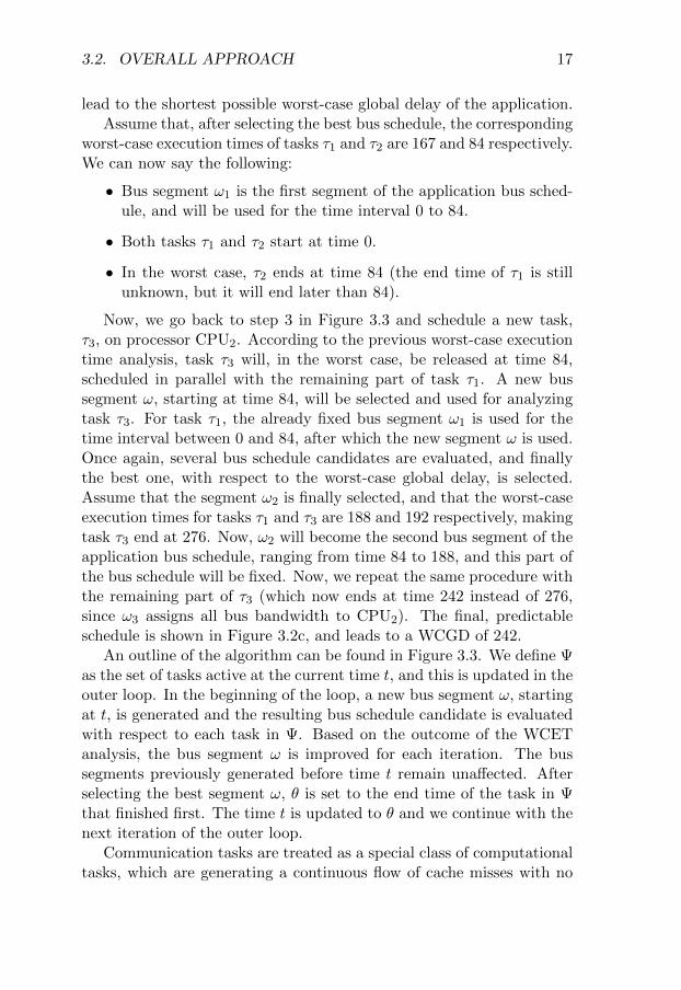
An outline of the algorithm can be found in Figure 3.3. We define Ψas the set of tasks active at the current time t, and this is updated in theouter loop. In the beginning of the loop, a new bus segment ω, startingat t, is generated and the resulting bus schedule candidate is evaluatedwith respect to each task in Ψ. Based on the outcome of the WCETanalysis, the bus segment ω is improved for each iteration. The bussegments previously generated before time t remain unaffected. Afterselecting the best segment ω, θ is set to the end time of the task in Ψthat finished first. The time t is updated to θ and we continue with thenext iteration of the outer loop.
Communication tasks are treated as a special class of computationaltasks, which are generating a continuous flow of cache misses with no

18 CHAPTER 3. PREDICTABILITY APPROACH
01: θ=002: while not all tasks scheduled
03: schedule new task at t ≥ θ04: Ψ=set of all tasks that are active at time t05: repeat
06: select bus segment ω for the
time interval starting at t07: determine the WCET of all tasks in Ψ08: until termination condition
09: θ=earliest time a task in Ψ finishes
10: end while
Figure 3.3 Overall approach
computational cycles in between. The number of cache misses is speci-fied such that the total amount of data transferred on the bus, due tothese misses, equals the maximum length of the explicit message. There-fore, from an analysis point of view, no special treatment is needed forexplicit communication. In the following, when we talk about cachemisses, it applies to both explicit and implicit communication.

4
Worst-Case Execution TimeAnalysis
In order to calculate the WCET of a task, the analysis needs to beaware of the TDMA bus, taking into account that processors must begranted the bus only during their assigned time slots. This chapter de-scribes the modifications required in order to adopt a traditional WCETalgorithm to our predictable approach, without increasing the overalltime-complexity.
4.1 TDMA-Based WCET Analysis
Performing worst-case execution time analysis with respect to a TDMAbus schedule requires not only knowledge about the number of cachemisses for a certain program path, but also their location with respectto time. Hence, traditional ILP-based methods for worst-case executiontime analysis cannot be applied. Instead, each memory access needs tobe considered with respect to the bus schedule, granting access to thebus only during the slots belonging to the requesting processor. How-ever, to collect the necessary information used by our worst-case execu-tion time analysis framework, the same techniques used in traditional
19

20 CHAPTER 4. WORST-CASE EXECUTION TIME ANALYSIS
methods can be utilized.
Calculating the worst-case execution time has to be done with re-spect to the particular hardware architecture on which the task beinganalyzed is going to be executed. Factors such as the instruction set,pipelining complexity, caches and so on must be taken into account bythe analysis. For an application running on a compositional architec-ture, the analysis can be divided into subproblems processed in a localfashion, for instance on basic block level. We can be sure that the lo-cal worst-case always contributes to the worst-case globally, allowingfor fast analysis techniques without the need to analyze every singleprogram path individually. This is, unfortunately, not the case whenusing noncompositional architectures. The presence of timing anomalieswill force the analysis to consider all possible program paths explicitly,naturally causing the analysis time to explode as the size of the tasksincrease.
For a predictable multiprocessor system with a shared communi-cation structure, as described in Chapter 2, it is necessary to searchthrough all feasible program paths and match each possible bus trans-fer to slots in the actual bus schedule, keeping track of exactly whena bus transfer is granted the bus in the worst case. This means thatthe execution time of a basic block will vary depending on when it isexecuted. Fortunately, for an application running on a compositionalarchitecture, efficient search-tree pruning techniques dramatically re-duce the search space, allowing for local analysis, just as for traditionalWCET techniques.
4.2 Compositional WCET Analysis Flow
A typical program flow for a WCET tool operating on compositionalarchitectures is shown in the left path of Figure 4.1 [33]. First, a con-trol flow graph (CFG) is generated. A value analysis is then performedto find program characteristics such as data address ranges and loopbounds. To take into account performance-enhancing features of mod-ern hardware, cache and pipeline analyses are carried out next. A pathanalysis identifies the feasible paths and an ILP formulation for calcu-lating the worst-case program path is then produced. The informationtraditionally provided in this ILP formulation is, however, not suffi-cient for calculating the WCET on a multiprocessor system since notonly the number of cache misses are needed for each basic block, but

4.2. COMPOSITIONAL WCET ANALYSIS FLOW 21
CFG Generation
Task
Value Analysis
Cache and PipelineAnalysis
Path Analysis
ILP Formulation
Evaluation(LP Solve)
Evaluation(Miss Mapping)
Traditional Approach
MPSoC Approach
Figure 4.1 WCET tool program flow
also their positions with respect to time. If necessary, an underlyingWCET tool has to be modified to provide this information. A morein-depth description can be found in the work published by Neikter [3].
Our TDMA-based approach for compositional WCET analysis isillustrated in the right path of Figure 4.1. After the path analysis, theinformation from the previous steps is used to calculate the worst-caseprogram path by mapping the cache misses to the corresponding busslots in the TDMA schedule. We will now show the idea behind thiswith a simple example.
4.2.1 Monoprocessor WCET Example
Consider a task τ executing on a system with two processors (processor1 and processor 2). The task is being mapped on processor 1, and hasstart time 0. First, an annotated control flow graph, as illustrated inFigure 4.2, is constructed. The rectangular elements B, C, H, E, F in

22 CHAPTER 4. WORST-CASE EXECUTION TIME ANALYSIS
ARoot
B025
C093
D
E09
F71
G
LoopBound: 3
H15
ISink
Figure 4.2 Example CFG
the graph represent basic blocks, and the circles A, D, G, I representcontrol nodes gluing them together. The loop starting at control node Gwill run at most three times, so the loop bound is consequently set to 3.The annotated numbers in the basic blocks represent consecutive cyclesof execution, in the worst case, not accessing the bus. For instance,basic block B will, when executed, immediately – after 0 clock cycles– issue a cache miss. After this, 2 cycles will be spent without busaccesses before the next (and last) cache miss occurs. Finally, 5 busaccess-free cycles will be executed before the basic block ends. Hence,the execution time of basic block B will be (0 + k1 + 2 + k2 + 5) wherek1 and k2 represent the transfer times of the first and second cache missrespectively. Note that usually, loop unrolling is performed in orderto decrease the pessimism of the analysis. This example is, however,purposely kept as simple as possible, and therefore the loop has notbeen unrolled.
For a typical monoprocessor system, all cache misses take the sameconstant amount of time to process, and the execution time of basicblock B would be known immediately. However, for multiprocessorarchitectures such as the one described in Chapter 2, we must calculatethe individual transfer times with respect to a given TDMA schedule.

4.2. COMPOSITIONAL WCET ANALYSIS FLOW 23
0 10 20 30 40 50 60 70
...
Slot belonging to processor 1
Slot belonging to processor 2
Figure 4.3 Example TDMA bus schedule
4.2.2 Multiprocessor WCET Example
Instead of a monoprocessor system, assume a multiprocessor system, asdescribed in Chapter 2, using the bus schedule in Figure 4.3. Processor1, on which the task is running, gets a bus slot of size 10 processorcycles periodically assigned to it every 20th cycle. In this particularexample, a cache miss takes 10 cycles for the bus to transfer, resultingin the bus being granted to processor 1 only at times t satisfying t ≡ 0(mod 20), where ≡ is the congruence operator.
To calculate the worst-case program path, we must evaluate all feasi-ble program paths in the control flow graph. In the very simple examplein Figure 4.2, there are 30 program paths1 to explore, growing exponen-tially with the number of branches and loop bounds. Fortunately, dueto the nature of the compositional architecture and the TDMA bus, notall of them have to be investigated explicitly. In fact, in a task graphwith all loops unrolled, each basic block would need to be investigatedexactly once, as will be explained in the following.
Let us denote the worst-case start time of a basic block Z by s(Z),and the end time in the worst case by e(Z). The execution time ofa basic block Z, in the worst case, is then defined as w(Z) = e(Z) −s(Z). Without considering bus conflicts, as in traditional methods,the worst-case execution time of the basic blocks would be wtrad(B) =27, wtrad(C) = 32, wtrad(E) = 19, wtrad(F) = 18 and wtrad(H) = 15.The corresponding worst-case program path becomes C,E,E,E,H re-sulting in a worst-case execution time of 27+19·3+15 = 104 clock cycles.However, this assumes that all cache misses take the same amount oftime to transfer, and this is false in a multiprocessor system with ashared communication structure. In our TDMA-based approach, theexecution time of a basic block depends on its start time in relation tothe bus schedule. We start from the root node and successively calculatethe execution time of each basic block with respect to the worst-case
12 + 22 + 23 + 24 = 30

24 CHAPTER 4. WORST-CASE EXECUTION TIME ANALYSIS
start time. At the same time, the worst-case path is calculated.With respect to the TDMA schedule in figure 4.3, the worst-case
start times of the basic blocks connected directly to the root node is 0,since they will never execute at any other time instant. The executiontime of block B, in the worst case, is w(B) = 0 + 10 + 2 + 18 + 5 = 35whereas the corresponding execution time of block C is w(C) = 0+10+9+11+3 = 33. Note that w(B) > w(C), even though the relation is theopposite in the traditional case above where wtrad(B) < wtrad(C). Inorder to decide which one of these two basic blocks is on the critical path,two very important observations must be made based on the predictablenature of the TDMA bus (and the compositionality considered in thissection).
1. The absolute end time of a basic block can never increase by lettingit start earlier. That is, a basic block Z with s(Z) = x ande(Z) = y, any start time x′ < x will result in an end time y′ ≤ y.The execution time of the particular basic block can increase, butthe increment can never exceed the difference x−x′ in start time.This means that for a basic block Z, the basic block will neverend later than e(Z) as long as it start before (or at) s(Z). Thisguarantees that the worst-case calculations will never be violated,no matter what program path is taken. Note that w(Z) is theexecution time in the worst case, with respect to e(Z), and thatthe time spent by executing Z can be greater than w(Z) for anearlier start time than s(Z).
2. Consider a basic block Z with worst-case start time s(Z) = x andworst-case end time e(Z) = y. If we, instead, assume a worst-casestart time of s(Z) = x′′ where x′′ > x, the corresponding resultingabsolute end time e(Z) = y′′ will always satisfy the relation y′′ ≥y. This means that the greatest assumed worst-case start times(Z) will also result in the greatest absolute end time e(Z).
Based on the second observation, we can be sure that the maximumabsolute end time for the basic block (E, F or H) succeeding B and Cwill be found when the worst-case start time is set to 35 rather than33. Therefore, we conclude that B is on the worst-case program pathand, since they are not part of a loop, B and C do not have to beinvestigated again.
Next follow three choices. We can enter the loop by executing eitherE or F, or we can go directly to H and end the task immediately. Due

4.3. NONCOMPOSITIONAL ANALYSIS 25
to observation 2 above, we can conclude that the worst-case absoluteend time of H, and thus the entire task, will be achieved when the loopiterates the maximum possible number of times, which is 3 iterations,since that will maximize s(H). Therefore, the next step is to calculatethe worst-case execution time for basic blocks E and F respectivelyfor each of the three iterations, before finally calculating the worst-case execution time of H. In the first iteration, the worst-case starttime is s(E1) = s(F1) = 35 and the execution times become w(E1) =0+15+9 = 24 and w(F1) = 7+28+1 = 36 for E and F respectively. Weconclude that the worst-case program path so far is B,F and the newstart time is set to s(E2) = s(F2) = 35 + 36 = 71. In the second loopiteration, we get w(E2) = 0 + 19 + 9 = 28 and w(F2) = 7 + 12 + 1 = 20.Hence, in this iteration, E contributes to the worst-case program pathand the new worst-case start time becomes s(E3) = s(F3) = 99. In thefinal iteration, the execution times are w(E3) = 0 + 11 + 9 = 20 andw(F3) = 7 + 24 + 1 = 32 respectively, resulting in the new worst-casestart time s(H) = 131. We now know that the worst-case program pathis B,F,E,F,H, and since H contains no cache misses, and thereforealways takes 15 cycles to execute, the WCET of the entire task is e(H) =146.
As shown in this example, in a loop-free control flow graph, eachbasic block has to be visited once. For control flow graphs containingloops, the number of investigations will be the same as for the casewhere all loops are unrolled according to their respective loop bounds.The result, when the graph is traversed, is a time-complexity not higherthan for traditional monoprocessor worst-case execution time analysistechniques.
4.3 Noncompositional Analysis
In the presence of timing anomalies, it is no longer possible to do localassumptions about the global worst case execution time. Therefore, forsuch architectures, every program path has to be analyzed explicitly.This is the case, not only for multiprocessor systems, but for any worst-case execution time framework operating on a noncompositional plat-form. Also, all steps in Figure 4.1, from the cache and pipeline analysesand forward, must be integrated since it, for noncompositional archi-tectures, is impossible to assume safe initial cache and pipeline statesfor a basic block, regardless of the allowed pessimism. Since also tradi-

26 CHAPTER 4. WORST-CASE EXECUTION TIME ANALYSIS
tional WCET analysis operating on noncompositional hardware has toperform a global search through all program paths, the modifications inorder to make it aware of the TDMA bus is, in theory, straight-forward.To adapt a traditional noncompositional WCET analysis technique tothe class of multiprocessor systems described in Chapter 2, for eachconsidered cache miss, the bus schedule has to be searched in order tofind the start and end times of the corresponding bus transfer. This op-eration is of linear complexity and will therefore not increase the total,already exponential, complexity of the traditional worst-case executiontime analysis.

5
Bus Schedule Optimization
Given any TDMA bus schedule, the WCET analysis framework de-scribed in Chapter 4 calculates a safe worst-case execution time. Thismeans that the WCET of a task is directly dependent on the bus sched-ule. This chapter describes how to generate a bus schedule, while sat-isfying various efficiency requirements. At the end of the chapter, wepresent experimental results showing the efficiency of our approach.
5.1 WCGD Optimization
Since the bus schedule is directly affecting the worst-case execution timeof the tasks, and consequently also the worst-case global delay of theapplication, it is important that it is chosen carefully. Ideally, whenconstructing the bus schedule, we would like to allocate a time slot foreach individual cache miss on the worst-case control flow path, grantingaccess to the bus immediately when it is requested. There are, however,two significant problems preventing us from doing this. The first one isthat several processors can issue a cache miss at the same time instant,creating conflicts on the bus. The second problem is that allocating bus
27

28 CHAPTER 5. BUS SCHEDULE OPTIMIZATION
slots for each individual memory transfer would create a very irregularbus schedule, requiring an unfeasible amount of memory space on thebus controller.
In order to solve the problem of irregular, memory consuming busschedules, some restrictions on the TDMA round complexity need to beimposed. For instance, an efficient strategy is to allow each processorto own a maximum number of slots per round. Other limitations canbe to let each round have the same slot order, or to force the slots in aspecific round to have the same size. In this chapter, we assume thatevery processor can own at most one bus slot per round. The slotsin a round can have different sizes, and the order can be set withoutrestrictions. However, it is straight-forward to adapt this algorithm tomore (or less) flexible bus schedule design rules. In addition to the mainalgorithm, we present a simplified algorithm for the special case whereall slots in a round must be of the same size.
The problem of handling cache miss conflicts is solved by distributingthe bus bandwidth such that the transfer times of cache misses, con-tributing directly to the worst-case global delay, are minimized. Thisis done in the inner loop of the overall approach outlined in Figure 3.3.For the optimization process, we start by defining a cost function thatestimates the worst-case global delay as a function of the bandwidthdistribution. A detailed description will follow in the next section.
5.2 Cost Function
Given a set of active tasks τi ∈ Ψ (see Figure 3.3), the goal is now togenerate a close to optimal bus segment schedule with respect to Ψ. Anoptimal bus schedule, however, is a bus schedule taking into accountthe global context, minimizing the global delay of the application. Thisglobal delay includes tasks not yet considered and for which no busschedule has been defined. This requires knowledge about future tasks,not yet analyzed, and, therefore, we must find ways to approximatetheir influence on the global delay.
In order to estimate the global delay, we first build a schedule Sλ
of the tasks not yet analyzed, using a list scheduling technique. Whenbuilding Sλ we approximate the WCET of each task by its respectiveworst-case execution time in the naive case, where no conflicts occuron the bus and any task can access the bus at any time. From nowon we refer to this conflict-free WCET as NWCET (Naive Worst-Case

5.2. COST FUNCTION 29
CPU
1C
PU2
(a) Gantt chart with respect to the NWCET of each task0 3 11 14 18 21
t
t
τ1
τ2
τ3
τ4
τ5
τ6
τ7
ΛC
PU1
CPU
2
(b) Gantt chart with optmized bus schedule for τ1
0 4 14 17 21 24
t
t
τ1
τ2
τ3
τ4
τ5
τ6
τ7
Λ
6 9
Λ+Δ
CPU
1C
PU2
(c) Gantt chart with optimized bus schedule for τ2
0 4 15 19 21 22
t
t
τ1
τ2
τ3
τ4
τ5
τ6
τ7
Λ
7 12
Λ+Δ
8
Figure 5.1 Estimating the global delay
Execution Time).
When optimizing the bus schedule for the tasks τ ∈ Ψ, we need anapproximation of how the WCET of one task τi ∈ Ψ affects the globaldelay. Let Di be the union of the set of all tasks depending directly onτi in the process graph, and the singleton set containing the first taskin Sλ that is scheduled on the same processor as τi. We now define thetail λi of a task τi recursively as:
• λi = 0, if Di = ∅
• λi = maxτj∈Di
(xj + λj), otherwise.
where xj = NWCETj if τj is a computation task. For communicationtasks, xj is an estimation of the communication time, depending on thelength of the message. Intuitively, λi can be seen as the length of thelongest (with respect to the NWCET) chain of tasks that are affectedby the execution time of τi. Without any loss of generality, in orderto simplify the presentation, only computation tasks are considered inthe examples of this section. Consider Figure 5.1a, illustrating a Ganttchart of tasks scheduled according to their NWCETs. Direct data de-pendencies exist between tasks τ4 & τ5, τ5 & τ6, and τ5 & τ7; hence,
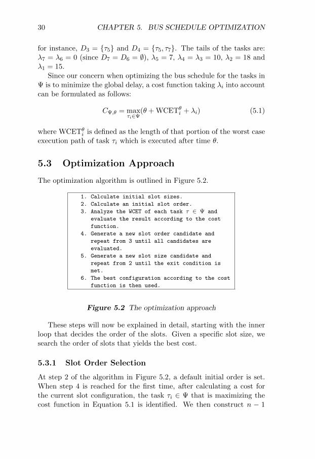
30 CHAPTER 5. BUS SCHEDULE OPTIMIZATION
for instance, D3 = τ5 and D4 = τ5, τ7. The tails of the tasks are:λ7 = λ6 = 0 (since D7 = D6 = ∅), λ5 = 7, λ4 = λ3 = 10, λ2 = 18 andλ1 = 15.
Since our concern when optimizing the bus schedule for the tasks inΨ is to minimize the global delay, a cost function taking λi into accountcan be formulated as follows:
CΨ,θ = maxτi∈Ψ
(θ + WCETθi + λi) (5.1)
where WCETθi is defined as the length of that portion of the worst case
execution path of task τi which is executed after time θ.
5.3 Optimization Approach
The optimization algorithm is outlined in Figure 5.2.
1. Calculate initial slot sizes.
2. Calculate an initial slot order.
3. Analyze the WCET of each task τ ∈ Ψ and
evaluate the result according to the cost
function.
4. Generate a new slot order candidate and
repeat from 3 until all candidates are
evaluated.
5. Generate a new slot size candidate and
repeat from 2 until the exit condition is
met.
6. The best configuration according to the cost
function is then used.
Figure 5.2 The optimization approach
These steps will now be explained in detail, starting with the innerloop that decides the order of the slots. Given a specific slot size, wesearch the order of slots that yields the best cost.
5.3.1 Slot Order Selection
At step 2 of the algorithm in Figure 5.2, a default initial order is set.When step 4 is reached for the first time, after calculating a cost forthe current slot configuration, the task τi ∈ Ψ that is maximizing thecost function in Equation 5.1 is identified. We then construct n − 1

5.3. OPTIMIZATION APPROACH 31
new bus schedule candidates, n being the number of tasks in the setΨ, by moving the slot corresponding to this task τi, one position at atime, within the TDMA round. The best configuration with respect tothe cost function is then selected. Next, we check if any new task τj ,different from τi, now has taken over the role of maximizing the costfunction. If so, the procedure is repeated, otherwise it is terminated.
5.3.2 Determination of Initial Slot Sizes
At step 1 of the algorithm in Figure 5.2, the initial slot sizes are dimen-sioned based on an estimation of how the slot size of an individual taskτi ∈ Ψ affects the global delay.
Consider λi, as defined in Section 5.2. Since it is a sum of theNWCETs of the tasks forming the tail of τi, it will never exceed theaccumulative WCET of the same sequence of tasks. Consequently, ifwe for all τi ∈ Ψ define
Λ = maxτi∈Ψ
(NWCETθi + λi) (5.2)
where NWCETθi is the NWCET of task τi ∈ Ψ counting from time θ,
a lower limit of the global delay can be calculated by θ + Λ. This isillustrated in Figure 5.1a, for θ = 0. Furthermore, let us define ∆ asthe amount by which the estimated global delay increases due to thetime each task τi ∈ Ψ has to wait for the bus.
See Figure 5.1b for an example. Contrary to Figure 5.1a, τ1 and τ2
are now considered using their real WCETs, calculated according to aparticular bus schedule (Ψ = τ1, τ2). The corresponding expansion∆ is 3 time units. Now, in order to minimize ∆, we want to express arelation between the global delay and the actual bus schedule. For taskτi ∈ Ψ, we define mi as the number of remaining cache misses on theworst case path, counting from time θ. Similarly, also counting from θ,li is defined as the sum of each code segment and can thus be seen asthe length of the task minus the time it spends using the bus or waitingfor it (both mi and li are determined by the WCET analysis). Hence,if we define the constant k as the time it takes to process a cache misswhen ignoring bus conflicts, we get
NWCETθi = li +mik (5.3)
As an example, consider Figure 5.3a showing a task execution trace, inthe case where no other tasks are competing for the bus. A black box

32 CHAPTER 5. BUS SCHEDULE OPTIMIZATION
τ1
0
τ2
0
δ1=32 k
(a) The anatomy of a taskδ2=30 δ
3=25 δ
4=28
δ'1=32 δ'
2=30 δ'
3=25
(b) The anatomy of a subtask
λ'2
τ'2
Θ2
t
t
Figure 5.3 Close-up of two tasks
represents the idle time, waiting for the transfer, due to a cache miss,to complete. In this example m1 = 4 and l1 = δ1 + δ2 + δ3 + δ4 = 115.
Let us now, with respect to the particular bus schedule, denote theaverage waiting time of task τi by di. That is, di is the average timetask τi spends waiting, due to other processors owning the bus and theactual time of the transfer itself, every time a cache miss has to betransferred on the bus. Then, analogous to Equation 5.3, the WCETof task τi, counting from time θ, can be calculated as
WCETθi = li +midi (5.4)
The dependency between a set of average waiting times di and a busschedule can be modeled as follows. Consider the distribution P, definedas the set p1, . . . , pn, where
∑pi = 1. The value of pi represents the
fraction of bus bandwidth that, according to a particular bus schedule,belongs to the processor running task τi ∈ Ψ. Given this model, theaverage waiting times can be rewritten as
di =1
pik (5.5)
Putting Equations 5.2, 5.4, and 5.5 together and noting that Λ has beencalculated as a maximum over all τi ∈ Ψ, we can formulate the following

5.3. OPTIMIZATION APPROACH 33
system of inequalities:
θ + l1 +m11
p1k + λ1 ≤ θ + Λ + ∆
...
θ + ln +mn1
pnk + λn ≤ θ + Λ + ∆
p1 + · · ·+ pn = 1
What we want is to find the bus bandwidth distribution P that resultsin the minimum ∆ satisfying the above system. Unfortunately, solvingthis system is difficult due to its enormous solution space. However, animportant observation that simplifies the process can be made, basedon the fact that the slot distribution is represented by continuous vari-ables p. Consider a configuration of p1, . . . , pn, ∆ satisfying the abovesystem, and where at least one of the inequalities are not satisfied byequality. We say that the corresponding task τi is not on the criticalpath with respect to the schedule, meaning that its corresponding pican be decreased, causing τi to expand over time without affecting theglobal delay. Since the values of p must sum to 1, decreasing pi, allowsfor increasing the percentage of the bus given to the tasks τ that are onthe critical path. Even though the decrease might be infinitesimal, thismakes the critical path shorter, and thus ∆ is reduced. Consequentlythe smallest ∆ that satisfies the system of inequalities is achieved whenevery inequality is satisfied by equality. As an example, consider Figure5.1b and note that τ5 is an element in both sets D3 and D4 accordingto the definition in Section 5.2. This means that τ5 is allowed to startfirst when both τ3 and τ4 have finished executing. Secondly, observethat τ5 is on the critical path, thus being a direct contributor to theglobal delay. Therefore, to minimize the global delay, we must make τ5
start as early as possible. In Figure 5.1b, the start time of τ5 is definedby the finishing time of τ4, which also is on the critical path. However,since there is a block of slack space between τ3 and τ5, we can reducethe execution time of τ2 and thus make τ4 finish earlier, by distributingmore bus bandwidth to the corresponding processor. This will make theexecution time of τ1 longer (since it receives less bus bandwidth), butas long as τ3 ends before τ4, the global delay will decrease. However, ifτ3 expands beyond the finishing point of τ4, the former will now be onthe critical path instead. Consequently, making task τ3 and τ4 end atthe same time, by distributing the bus bandwidth such that the sizes of

34 CHAPTER 5. BUS SCHEDULE OPTIMIZATION
CPU1
CPU2
CPU3
(a)
(b)
(c)
Figure 5.4 Calculation of new slot sizes
τ1 and τ2 are adjusted properly, will result in the earliest possible starttime of τ5, minimizing ∆. In this case the inequalities corresponding toboth τ1 and τ2 are satisfied by equality. Such a distribution is illustratedin Figure 5.1c.
The resulting system consists of n+ 1 equations and n+ 1 variables(p1, . . . , pn and ∆), meaning that it has exactly one solution, andeven though it is nonlinear, it is simple to solve. Using the resultingdistribution, a corresponding initial TDMA bus schedule is calculatedby setting the slot sizes to values proportional to P .
5.3.3 Generation of New Slot Size Candidates
One of the possible problems with the slot sizes defined as in Section5.3.2 is the following: if one processor gets a very small share of the busbandwidth, the slot sizes assigned to the other processors can becomevery large, possibly resulting in long wait times. By reducing the sizesof the larger slots while trying to keep their mutual proportions, thisproblem can be avoided.
We illustrate the idea with an example. Consider a round consistingof three slots ordered as in Figure 5.4a. The slot sizes have been dimen-sioned according to a bus distribution P = 0.49, 0.33, 0.18, calculatedusing the method in Section 5.3.2. The smallest slot, belonging to CPU3, has been set to the minimum slot size k, and the remaining slot sizesare dimensioned proportionally 1 as multiples of k. Consequently, theinitial slot sizes become 3k, 2k and k. In order to generate the next setof candidate slot sizes, we define P ′ as the actual bus distribution ofthe generated round. Considering the actual slot sizes, the bus distri-bution becomes P ′ = 0.50, 0.33, 0.17. Since very large slots assignedto a certain processor can introduce long wait times for tasks running
1While slot sizes, in theory, do not have to be multiples of the minimum slot sizek, in practice this is preferred as it avoids introducing unnecessary slack on the bus.

5.3. OPTIMIZATION APPROACH 35
on other processors, we want to decrease the size of slots, but still keepclose to the proportions defined by the bus distribution P . Consideronce again Figure 5.4a. Since, p′1− p1 > p′2− p2 > p′3− p3, we concludethat slot 1 has the maximum deviation from its supposed value. Hence,as illustrated in Figure 5.4b, the size of slot 1 is decreased one unit.This slot size configuration corresponds to a new actual distributionP ′ = 0.40, 0.40, 0.20. Now p′2 − p2 > p′3 − p3 > p′1 − p1, hence thesize of slot 2 is decreased one unit and the result is shown in Figure5.4c. Note that in the next iteration, p′3 − p3 > p′1 − p1 > p′2 − p2, butsince slot 3 cannot be further decreased, we recalculate both P and P ′,now excluding this slot. The resulting sets are P = 0.60, 0.40 andP ′ = 0.67, 0.33, and hence slot 1 is decreased one unit. From nowon, only slot 1 and 2 are considered, and the remaining procedure iscarried out in exactly the same way as before. When this procedureis continued as above, all slot sizes will converge towards k which, ofcourse, is not the desired result. Hence, after each iteration, the costfunction (Equation 5.1) is evaluated and the process is continued onlyuntil no improvement is registered for a specified number π of itera-tions. The best ever slot sizes (with respect to the cost function) are,finally, selected. Accepting a number of steps without improvementmakes it possible to escape certain local minima (in our experiments weuse 8 < π < 40, depending on the number of processors).
5.3.4 Density Regions
A problem with the technique presented above is that it assumes thatthe cache misses are evenly distributed throughout the task. For mosttasks, this is not the case in reality. A solution to this problem isto analyze the internal cache miss structure of the actual task and,accordingly, divide the worst case path into disjunct intervals, so calleddensity regions. A density region is defined as an interval of the pathwhere the distance between consecutive cache misses (δ in Figure 5.3)does not differ more than a specified number. In this context, if wedenote by α the average time between two consecutive cache misses(inside a region), the density of a region is defined as 1
α+1 . A regionwith high density, close to 1, has very frequent cache misses, while theopposite holds for a low-density region.
Consequently, in the beginning of the optimization loop, we identifythe next density region for each task τi ∈ Ψ. Now, instead of construct-ing a bus schedule with respect to each entire task τi ∈ Ψ, only the

36 CHAPTER 5. BUS SCHEDULE OPTIMIZATION
interval [θ..Θi) is considered, with Θi representing the end of the den-sity region. We call this interval of the task a subtask since it will betreated as a task of its own. Figure 5.3b shows a task τ2 with two den-sity regions, the first one corresponding to the subtask τ ′2. The tail of τ ′2is calculated as λ′2 = λ′′2 + λ2, with λ′′2 being defined as the NWCET ofτ2 counting from Θ2. Furthermore, in this particular example m′2 = 3and l′2 = δ′1 + δ′2 + δ′3 = 87.
Consider Figure 3.3 illustrating the overall approach. Analogous tothe case where entire tasks are analyzed, when a bus schedule for thecurrent bus segment has been decided, θ′ will be set to the finish time ofthe first subtask. Just as before, the entire procedure is then repeatedfor θ = θ′.
However, modifying the bus schedule can cause the worst-case con-trol flow path to change. Therefore, the entire cache miss structurecan be transformed during the optimization procedure (lines 4 and 5 inFigure 5.2), resulting in possible changes with respect to both subtaskdensity and size. We solve this problem by using an iterative approach,adapting the bus schedule to possible changes of the subtask structurewhile making sure that the total cost is decreasing. This procedure willbe described in the following paragraphs.
Subtask Evaluation
First, let us in this context define two different cost functions, bothbased on Equation 5.1. Let τ
′endi be the end time of subtask τ ′i , and
define τ′end as:
τ′end = min
τi∈Ψ(τ
′endi ) (5.6)
Furthermore, let NWCETτ′end
i be the NWCET of the task τi, count-ing from τ
′end to the end of the task. The subtask cost C′Ψ,θ can now
be defined as:
C′Ψ,θ = max
τi∈Ψ(τ
′end + NWCETτ′end
i + λi) (5.7)
Hence, the subtask cost is a straight-forward adaption of the cost func-tion in Equation 5.1 to the concept of subtasks. Instead of using theworst-case execution time of the entire task, only the part correspond-ing to the first density region after time θ is considered. The rest of
5.3. OPTIMIZATION APPROACH 37
the task, from the end of the first density region to the end of the en-tire task, is accounted for in the tail, with respect to its correspondingNWCET.
In order to more accurately approximate how the subtask affects theworst-case global delay, we also introduce its complementary task cost
C′′Ψ,θ in addition to the subtask cost. Let WCETτ
′end
i be the worst-case
execution time of task τi starting from time τ′end. We here assume that
WCETτ′end
i has been calculated with respect to a tailored bus segment,starting after τ
′end. The bus schedule representing this bus segmentis calculated considering the cache miss structure of the correspondingpart of the task, for instance by using the algorithm described in Section5.3.2 for calculating initial slot sizes. This way we can approximate thetransfer delays of the cache misses between τ
′end and the end of the task,instead of using the corresponding NWCET (as is done when calculatingthe subtask cost). The complementary task cost can be defined as:
C′′Ψ,θ = max
τi∈Ψ(τ
′end + WCETτ′end
i + λi) (5.8)
Note that the only difference between this cost function and theprevious one in Equation 5.7 is that we now use a calculated WCET forthe remaining part of the task, instead of the NWCET. Consequently,the complementary task cost is always greater than or equal to thesubtask cost. The problem with using the NWCET, as done whencalculating the subtask cost, is that small subtasks tend to be favored.The complimentary cost is more precise, but also more time-consumingto calculate. Therefore the idea is to use it only when necessary.
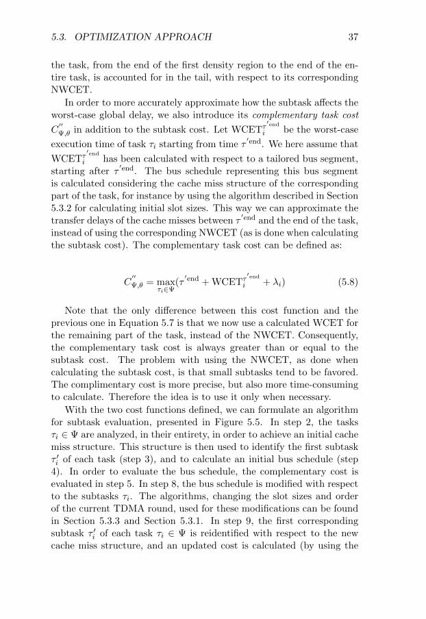
With the two cost functions defined, we can formulate an algorithmfor subtask evaluation, presented in Figure 5.5. In step 2, the tasksτi ∈ Ψ are analyzed, in their entirety, in order to achieve an initial cachemiss structure. This structure is then used to identify the first subtaskτ ′i of each task (step 3), and to calculate an initial bus schedule (step4). In order to evaluate the bus schedule, the complementary cost isevaluated in step 5. In step 8, the bus schedule is modified with respectto the subtasks τi. The algorithms, changing the slot sizes and orderof the current TDMA round, used for these modifications can be foundin Section 5.3.3 and Section 5.3.1. In step 9, the first correspondingsubtask τ ′i of each task τi ∈ Ψ is reidentified with respect to the newcache miss structure, and an updated cost is calculated (by using the

38 CHAPTER 5. BUS SCHEDULE OPTIMIZATION
less expensive subtask cost function). If this cost is an improvement ofthe previous cost2, we also evaluate the complementary cost C
′′Ψ,θ. If
the new complementary cost is lower than the best cost Cbestinner found so
far in the inner loop, we update Cbestinner to this new lowest cost.
We then try to modify the bus schedule further until no more im-provements are found (steps 8-12). Consequently, reaching step 13means two things. Either we have found the best bus schedule, or theworst-case control flow path has changed during the iterations, result-ing in a different cache miss structure, not suitable for the generatedbus schedule (again, note that the steps 8-12 try to improve the ini-tial sizes calculated, with respect to a specific density, in step 4). IfCbest
inner = Cbestouter, we did not manage to improve the existing best cost
from the last time the inner loop was visited, and the algorithm ishalted. If Cbest
inner < Cbestouter, on the other hand, we identify new subtasks
with respect to the improved bus schedule (step 3), and repeat the pro-cedure. Note that this algorithm will always converge since it neveraccepts solutions that lead to higher costs.
5.4 Simplified Algorithm
For the case where all slots of a round have to be of the same, round-specific size, calculating the distribution P makes little sense. Therefore,we also propose a simpler, but quality-wise equally efficient algorithm,tailor-made for this class of more limited bus schedules. The slot order-ing mechanisms are still the same as for the main algorithm, but theprocedures for calculating the slot sizes are now vastly simplified. Thealgorithm is summarized in Figure 5.6.
In step 1, we start by using the smallest possible slot size, since thiswill minimize the maximum transfer delay. Next, an initial slot order,chosen arbitrarily, is specified in step 2. The slot order candidates arethen generated just as in the general algorithm, by changing the positionof the slot belonging to the processor on the critical path. After findingthe best order for a particular slot size, the latter is modified by, forinstance, increasing it k steps. After an appropriate slot size is found, itcan also be ”‘fine tuned”’ by increasing or decreasing the size by a verysmall amount, less than k. Since all processors get the same amount
2In the opposite case, for which no improvement of the cost was made, there isno need to calculate C
′′Ψ,θ since C
′Ψ,θ < C
′′Ψ,θ.

5.5. MEMORY CONSUMPTION 39
1. Set Cbestouter = ∞.
2. Calculate initial slot sizes with respect
to all tasks τi ∈ Ψ.
3. For each task τi ∈ Ψ, calculate the WCET
and identify the corresponding first
subtask τ ′i.4. Calculate the initial slot sizes with
respect to the subtasks τ ′i.5. Calculate the complementary task cost
C′′Ψ,θ.
6. If C′′Ψ,θ < Cbest
outer, set Cbestouter = C
′′Ψ,θ.
7. Set Cbestinner = Cbest
outer.
8. Modify the bus schedule with respect to
the cache miss structure of τ ′i.9. Once again, for each task τi ∈ Ψ,
calculate the WCET and identify the first
corresponding subtask τ ′i.
10. Calculate the subtask cost C′Ψ,θ.
11. If C′Ψ,θ < Cbest
inner, calculate the
complementary task cost C′′Ψ,θ and, if
C′′Ψ,θ < Cbest
inner, set Cbestinner = C
′′Ψ,θ.
12. Repeat from 8 until no improvements have
been made for N iterations.
13. If Cbestinner < Cbest
outer then set Cbestouter = Cbest
inner
and goto 3
14. Use the bus schedule corresponding to
Cbestouter for the interval between θ and the
end time of the subtask that finished
first, and update θ to this end time.
Figure 5.5 Subtask evaluation algorithm
of bus bandwidth, the concept of density regions is not useful in thissimplified approach.
5.5 Memory Consumption
As stated in Section 2.3, a TDMA bus schedule is composed of segments.Therefore, the amount of memory space needed to store the bus scheduleis defined by the number of segments and the complexity restrictionsimposed, by the system designer, on the underlying TDMA rounds. Inorder to calculate an upper bound on the number of segments needed,we make the observation that a new segment is created at every time

40 CHAPTER 5. BUS SCHEDULE OPTIMIZATION
1. Initialize the slot sizes to the minimum
size k.2. Calculate an initial slot order.
3. Analyze the WCET of each task τ ∈ Ψ and
evaluate the result according to the cost
function.
4. Generate a new slot order candidate and
repeat from 3 until all candidates are
evaluated.
5. Increase the slot sizes one step.
6. If no improvements were achieved during a
specified number of iterations then exit.
Otherwise repeat from 2.
7. The best configuration according to the
cost function is then used.
Figure 5.6 The simplified optimization approach
t when at least one task starts or finishes. For the case when densityregions are not used, these are also the only times when a new segmentwill be created. Hence, an upper bound on the number of segments is2|Π|, where Π is the set of all tasks as defined in Chapter 2.
When using density regions, the start and finish of every region canresult in a new segment each. Therefore, tasks divided into very manysmall density regions will result in bus schedules consuming more mem-ory. A straight-forward solution is to limit, according to the availablecontroller memory, the minimum size of a density region. For instance,if the minimum density region size for a task τi is x% of the task lengthli as defined above, the number of generated segments becomes at most2|Π|100
x .
5.6 Experimental Results
The complete flow illustrated in Figure 3.3 has been implemented andused as a platform for the experiments presented in this section. The busschedule synthesis was carried out on a general purpose PC with a dualcore Pentium 4 processor, running at 2.8 GHz. We have developed aWCET analysis tool, using SymTA/P from Braunschweig University asstarting point, based on the considerations in Chapter 4. A system-on-chip design according to Chapter 2, consisting of several ARM7 cores, isassumed for the worst-case execution time analysis. For these examples,

5.6. EXPERIMENTAL RESULTS 41
0 10
Slot start Owner0 CPU1
10 CPU240 CPU160 CPU270 CPU1
40 60
...Bus
Slot belonging to CPU1Slot belonging to CPU2
... ...
70
Figure 5.7 BSA1 bus schedule
we have assumed that 12 clock cycles are required to handle a memoryaccess due to a cache miss.
5.6.1 Bus Schedule Approaches
To evaluate our algorithms, we defined four bus schedule approachesof varying complexity. The least restrictive approach, BSA1, imposesno restrictions at all and is therefore mostly of interest for comparisonswith the other approaches. Since there is no requirement for regularity,a BSA1 schedule is composed by only one segment, consisting of a(very complex) round having the same size as the segment itself. Eachprocessor can own any number of slots of different sizes, and the orderof the slots is arbitrary. An example of a BSA1 bus schedule and itstable representation can be found in Figure 5.7.
With the more restrictive BSA2, each processor can own at most onebus slot per round. However, the slots in a round can still have differentsizes, and the order can be set arbitrarily. Imposing this restriction onthe round dramatically decreases the memory needed to store the busschedule, since the regularity can be used to store it in an efficientfashion. An example of a BSA2 bus schedule is depicted in Figure5.8. The first segment starts at time unit 0 and ends at time unit 60,immediately followed by the second segment. The main algorithm inthis chapter assumes that a BSA2 bus schedule is used.
BSA3 is as BSA2 but with the additional restriction that all slots

42 CHAPTER 5. BUS SCHEDULE OPTIMIZATION
0 10
Slot sizeOwner10CPU120CPU210CPU210CPU1......
30 40
...Bus
Slot belonging to CPU1Slot belonging to CPU2
60 70 80 90 100
Segment start
0
60
...
Figure 5.8 BSA2 bus schedule
0 10
Slot sizeOwner
10CPU2CPU1
20CPU1CPU2
......
20 30
...Bus
Slot belonging to CPU1Slot belonging to CPU2
40 60 80 100 120
Segment start
0
40
...
Figure 5.9 BSA3 bus schedule
in a round must be of the same size, regardless of owner. This furtherdecreases the amount of memory required on the bus arbiter, since onlyone size has to be stored for each round, regardless of the number ofslots. The order is, however, still arbitrary, just as for BSA2. Anexample is illustrated in Figure 5.9. The simplified algorithm explainedin this chapter operates on BSA3 bus schedules.
We have also defined a fourth approach, BSA4, which is as BSA3but with the very strong restriction of allowing only bus schedules con-stituted by one segment (and thus one round). This requires almost no
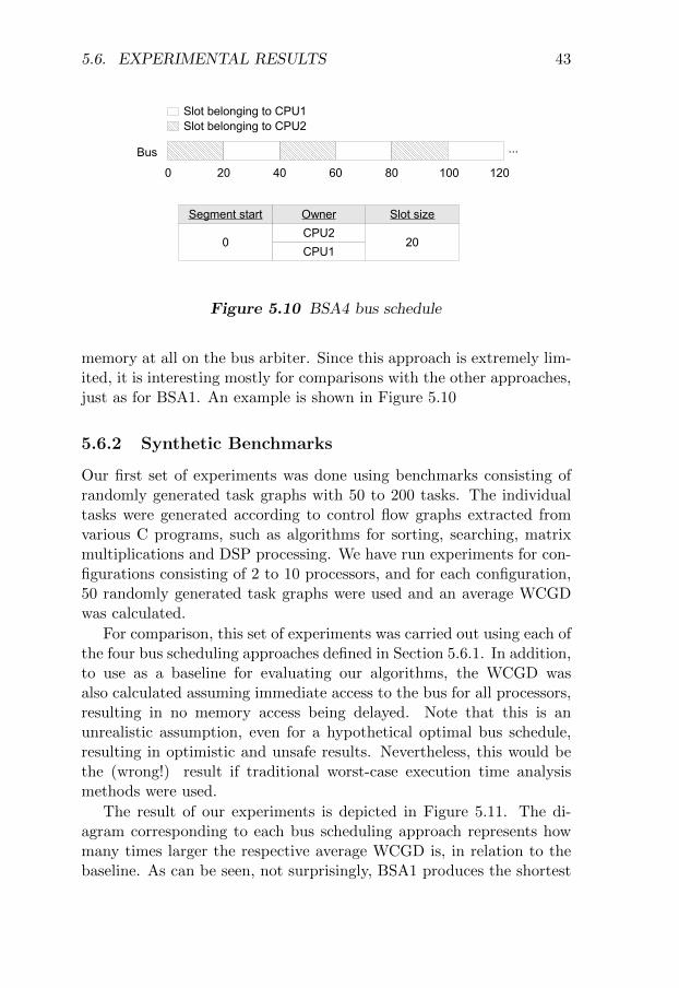
5.6. EXPERIMENTAL RESULTS 43
0 20
Slot sizeOwner
20CPU2CPU1
...Bus
Slot belonging to CPU1Slot belonging to CPU2
40 60 80 100 120
Segment start
0
Figure 5.10 BSA4 bus schedule
memory at all on the bus arbiter. Since this approach is extremely lim-ited, it is interesting mostly for comparisons with the other approaches,just as for BSA1. An example is shown in Figure 5.10
5.6.2 Synthetic Benchmarks
Our first set of experiments was done using benchmarks consisting ofrandomly generated task graphs with 50 to 200 tasks. The individualtasks were generated according to control flow graphs extracted fromvarious C programs, such as algorithms for sorting, searching, matrixmultiplications and DSP processing. We have run experiments for con-figurations consisting of 2 to 10 processors, and for each configuration,50 randomly generated task graphs were used and an average WCGDwas calculated.
For comparison, this set of experiments was carried out using each ofthe four bus scheduling approaches defined in Section 5.6.1. In addition,to use as a baseline for evaluating our algorithms, the WCGD wasalso calculated assuming immediate access to the bus for all processors,resulting in no memory access being delayed. Note that this is anunrealistic assumption, even for a hypothetical optimal bus schedule,resulting in optimistic and unsafe results. Nevertheless, this would bethe (wrong!) result if traditional worst-case execution time analysismethods were used.
The result of our experiments is depicted in Figure 5.11. The di-agram corresponding to each bus scheduling approach represents howmany times larger the respective average WCGD is, in relation to thebaseline. As can be seen, not surprisingly, BSA1 produces the shortest

44 CHAPTER 5. BUS SCHEDULE OPTIMIZATION
1 2 3 4 5 6 7 8 9 101
1,1
1,2
1,3
1,4
1,5
1,6
1,7
1,8
1,9
2
BSA1BSA2BSA3BSA4
Number of Processors
Nor
mal
ized
Sch
edul
e Le
ngth
Figure 5.11 Four bus access policies
worst-case global delays. This is expected, since the corresponding busschedules have no restrictions with respect to flexibility. The resultsproduced by BSA2 and BSA3 are, however, not at all far behind. Thisshows that the price for obtaining regular bus schedules, which can befitted into memories with a relatively small capacity, is very low. Thepoor flexibility provided by BSA4, on the other hand, is not enough,and for large bus schedules, the results become inferior.
In a second set of experiments, we have compared the BSA2 andBSA3 bus scheduling approaches, since they are the important alterna-tives from a practical viewpoint. In particular, we were interested inthe efficiency of these policies for applications with different cache misspatterns. A cache miss pattern of a particular task is, in this context,characterized by the standard deviation of the set of time-intervals be-tween all consecutive cache misses. Three classes of applications, eachone representing a different level of cache miss irregularity, were cre-ated. Every application was composed, according to a randomized taskgraph, by 20 randomly generated tasks, and each class contained 30applications. For all tasks, the average distance between consecutivecaches misses was 73 clock cycles.
The first class of applications was generated with a uniformly dis-tributed cache miss pattern, corresponding to a standard deviation of

5.6. EXPERIMENTAL RESULTS 45
0 clock cycles. The other two classes had a more irregular cache missstructure, corresponding to standard deviations of 50 and 150 clock cy-cles, respectively. Just as for the previous set of examples, the unsafetraditional case, where no processor ever has to wait for the bus, is usedas a baseline. A comparison of the resulting average worst-case globaldelays is shown in Figure 5.12. It is expected that the two approachesproduce the same worst-case global delays for very regular cache missstructures since, most of the time, all processors will demand an equalamount of bus bandwidth. However, as the irregularity of the cachemiss structure increases, the ability of BSA2 to distribute the band-width more freely becomes more and more of an advantage.
We also carried out a third set of experiments, demonstrating theefficiency of the successive steps of our main bus access optimizationalgorithm. The same three classes of applications were used as for theprevious set, as well as the same baseline. The results are presented inFigure 5.13. The ISS bar represents the average worst-case global delayobtained using the initial slot sizes, calculated as described in Section5.3.2. The SSA bar corresponds to the average WCGD after slot sizeadjustments, as described in Section 5.3.3, have been performed as well.Finally, the DS bar shows the result of also applying the concept ofdensity regions, according to Section 5.3.4, in addition to the previoustwo steps. As expected, density regions are efficient for irregular cachemiss patterns, but do not help if the structure is uniformly distributed.
The execution time, for the whole flow, of an example consisting of100 tasks on 10 processors is 120 minutes for the BSA2 algorithm and5 minutes for the simplified BSA3 version.
5.6.3 Real-Life Example
In order to validate the real-world applicability of this approach, wehave also analyzed a smart phone. It consists of a GSM encoder, GSMdecoder and an MP3 decoder, mapped on four ARM7 processors. TheGSM encoder and decoder are mapped on one processor each, whereasthe MP3 decoder is mapped on two processors. The software appli-cations have been partitioned into 64 tasks, and the size of one suchtask is between 70 and 1304 lines of C code for the GSM codec, and200 and 2035 lines for the MP3 decoder. We have assumed a 4-wayset associative instruction cache with a size of 4 kilobytes and a directmapped data cache of the same size. The worst-case global delay wascalculated using the four bus scheduling approaches defined in Section

46 CHAPTER 5. BUS SCHEDULE OPTIMIZATION
0 50 1501
1,1
1,2
1,3
1,4
1,5
1,6
BSA3BSA2
Standard Deviation
Nor
mal
ized
Sch
edul
e Le
ngth
Figure 5.12 Comparison between BSA2 and BSA3
0 50 1501
1,1
1,2
1,3
1,4
1,5
1,6
1,7
1,8
ISSSSADS
Standard Deviation
Nor
mal
ized
Sch
edul
e Le
ngth
Figure 5.13 BSA2 optimization steps
5.6.1. For comparison, we also calculated the WCGD assuming, un-realistically, immediate access to the bus for each processor, as doneby traditional worst-case execution time analysis techniques. Table 5.1shows, for each of the four bus scheduling approaches, how many timeslarger the obtained safe worst-case global delay is compared to the un-realistic counterpart. As can be seen, the results are coherent with theexperiments in Section 5.6.2.

5.6. EXPERIMENTAL RESULTS 47
BSA1 BSA2 BSA3 BSA4
1.17 1.31 1.33 1.62
Table 5.1 Results for the smart phone

48 CHAPTER 5. BUS SCHEDULE OPTIMIZATION

6
Worst/Average-CaseOptimization
When optimizing a system platform for a hard real-time application, thegoal is, traditionally, to minimize the worst-case global delay. However,the worst-case program path of an application is in most cases takenvery seldom, and doing so generally leads to a much longer executiontime than what can be expected on average, resulting in a gap betweenthe WCGD and the average-case global delay (ACGD). Therefore, whendesigning periodic systems, there will be a significant interval of timeafter the program has finished until the next period starts. During thistime interval, the processors are free to be used for anything, as longas they are ready and available at the start of the new period. Thus,instead of just letting them be idle, doing nothing, we can utilize thisslack for performing computations not requiring strict predictability, orwe can just shut off the processors to save energy. Consequently, itcan be of great interest that the average-case global delay is as short aspossible, even for hard real-time systems. In this chapter, we present anefficient algorithm for obtaining predictable real-time applications witha low average-case global delay, while still keeping the WCGD close toa minimum.
49

50 CHAPTER 6. WORST/AVERAGE-CASE OPTIMIZATION
6.1 Motivation
Consider the hard real-time application in Figure 6.1a, composed of thethree tasks τ1, τ2 and τ3 running on two processors. The applicationis periodically executed with a period equal to the worst-case globaldelay. After finishing the last computation, the processors are poweredoff, until the start of the next period, to save energy. Consequently, inthe average case, the processors are shut off between the time instantsACGD and WCGD, and since the goal is to reduce the power consump-tion as much as possible, we would like to maximize this time interval.However, we also want to have a short period and, therefore, the worst-case global delay must remain small. Hence, optimizing for the averagecase without caring for the worst case is not suitable for this kind ofsystems. On the other hand, if we optimize for the ACGD while alsomaking sure that the WCGD is kept at a near-minimum, it is possi-ble to benefit from a substantial reduction of power consumption whileextending the application period only marginally. This is exactly thecase in Figure 6.1b, where it can be seen that the energy consumed forrunning the application is dramatically reduced, but since the WCGDis increased only by a small amount, the application period can still bekept low.
The interval between the end time of the application and the WCGDcan, obviously, also be used for other purposes than switching off theprocessors. In Figure 6.1c, we have used the remaining time, after theend of the application, for running best effort calculations, representedby the tasks τ4, τ5 and τ6. These tasks can, if needed, be preempted atthe end of the application period.
Another example, outside the traditional hard real-time domain, canbe found in Figure 6.2. The application, consisting of the three tasksτ1, τ2 and τ3 running on two processors is, at the end of its execution,writing a produced result to a FIFO buffer and is then immediatelyrestarted. An external consumer is periodically reading data from theother end of the buffer. For such systems, a small ACGD allows forhigh data rates, but in order to guarantee a minimum rate and to helpthe system designer dimension the buffer, the WCGD must be knownand, preferably, be small as well.

6.1. MOTIVATION 51
CPU1
CPU2
τ1
τ2
τ3
WCGDACGD
off
off
a) Optimized for the WCGD
CPU1
CPU2
τ1
τ2
τ3
WCGD'ACGD'
off
off
b) Optimized for the WCGD and ACGD
CPU1
CPU2
τ1
τ2
τ3
WCGD'ACGD'
τ4
τ5
c) Performing additional best effort calculations
τ6
Figure 6.1 Motivational example for a hard real-time system
rt
rt-n
Data is periodically fetched
CP
U1
CP
U2
τ1
τ2
τ3
WCGD'ACGD'
rt
rt-1
rt-2
...r
t-n
Buffer
Figure 6.2 Motivational example for a buffer-based system

52 CHAPTER 6. WORST/AVERAGE-CASE OPTIMIZATION
6.2 Average-Case Execution Time Estimation
When calculating the worst-case execution time of a task, one tries tofind the worst-case program path with respect to the specified bus sched-ule. The optimization algorithm then locates where, with respect to theworst-case program path, to allocate bandwidth. This technique is notdirectly applicable to average-case execution time analysis, since there isgenerally no particular program path corresponding to the average-caseexecution time of a task.
To evaluate how good a bus schedule is from the point of view of theaverage-case execution time, the application has to be executed a largenumber of times so that the end time of each run can be recorded andused to calculate a mean. This is, naturally, a rather time-consumingprocess, and therefore, using this method repetitively inside an opti-mization loop leads to unmanageably long analysis times. Also, in orderfor the optimization algorithm to know where to allocate bus bandwidthfor a certain task, the locations, with respect to time, of the cache missesfor an average execution of the task have to be approximated. We solvethese two problems by using a histogram-based technique, where taskmeasurement data is used to create task profiles then given as input tothe optimization algorithm.
In order to build the memory access histogram, N sets of input dataare generated for each task. This data is randomized with respect to adistribution representing typical input patterns for the particular taskin question. Every task is then executed, in isolation, N times and,for each execution, a trace file containing the locations of the cachemisses is generated. Using this information, we want to find out where,in time, cache misses are most likely to occur so that bus bandwidthcan be assigned accordingly. This is done by building, for each task,a histogram over bus accesses in time (not considering the actual timespent waiting for and using the bus), with respect to all N measuredexecutions.
Figure 6.3 shows an example of a histogram based on 1000 execu-tions. The y-value of the histogram denotes how many of the N mea-sured executions of the task accessed the bus during the time intervalrepresented by the corresponding x-value. For instance, in this exam-ple, it can be seen that all measured executions access the bus at thevery start of the task due to instruction cache misses. During the timeregions denoted by t1, t2, t3 and t4, most measured executions accessthe bus, and therefore chances are high that so will be the case during

6.2. AVERAGE-CASE EXECUTION TIME ESTIMATION 53
an average execution of the task. Consequently, making sure that thetask gets a lot of bandwidth during these time periods is most likely agood idea.
Time
Frequency
t1
t2
t3
t4
0
1000
Figure 6.3 Example histogram for 1000 executions
Given the histogram and a specified bus schedule, we can obtain anestimation of the average-case task execution time with respect to thebus schedule. By using the frequency data on the y-axis, a set of NH
representative hypothetical program paths can be constructed. Thesehypothetical paths can then be used to approximate the average-caseexecution time by analyzing their respective global delay and calculatingthe mean. We will illustrate how this is done by a simple example.
100 20 30 40 500
12
Figure 6.4 Example histogram for 12 executions
Consider the histogram in Figure 6.4. In this example, 12 executionshave been carried out (N = 12), and we want to use this informationto estimate the average-case execution time of the measured task withrespect to a certain bus schedule. For each execution of the task duringthe construction of the histogram, the corresponding execution pathlength, defined as the end-to-end delay excluding bus transfer times, andthe number of cache misses are recorded. This information is sorted,

54 CHAPTER 6. WORST/AVERAGE-CASE OPTIMIZATION
with respect to the execution path length, and presented in Figure 6.5.We can see that the shortest execution path was 8 clock cycles long(excluding transfer times) and had 5 cache misses. The longest path,on the other hand, measured 60 clock cycles and generated 15 cachemisses.
Path Length Number of Misses8 59 611 512 818 928 1232 1134 1239 1148 1457 1660 15
Figure 6.5 Example table for hypothetical path classification
For this example, we want to create three hypothetical control flowpaths (NH = 3). Consequently, we start by dividing the measured exe-cution paths in Figure 6.5 into three equally sized groups, with respectto their execution path lengths. The first group (Group 1) contains thefour shortest executions (lengths 8, 9, 11 and 12), whereas the two othergroups (Group 2 and Group 3) contain the medium-length executions(lengths 18, 28, 32, 34) and the longest executions (lengths 39, 48, 57,60), respectively. The idea is to now construct a hypothetical executionpath for each of the three groups, capturing their characteristics.
First, we want to compute the representative execution path lengthand corresponding number of cache misses for each of the three hy-pothetical paths. This is done by calculating the averages for eachgroup. The hypothetical path corresponding to Group 1 will thus havean execution path length of (8 + 9 + 11 + 12)/4 = 10 and be assigned(5 + 6 + 5 + 8)/4 = 6 cache misses. The path corresponding to Group2 will have a length of 28 with 11 cache misses, and for Group 3 thecorresponding values will be 51 and 14, respectively. We can now, withrespect to the histogram, assign cache misses to the hypothetical paths.

6.2. AVERAGE-CASE EXECUTION TIME ESTIMATION 55
We will show how to do this for Group 1, with the shortest executionpath lengths.
Position Misses P r1
r2
r3
Included
0 12 1.00 0.13 - - Yes3 8 0.67 0.71 0.75 0.55 Yes2 7 0.58 0.53 - - Yes1 6 0.50 0.22 - - Yes4 5 0.42 0.96 0.46 - No5 4 0.33 0.31 - - Yes9 4 0.33 0.76 0.34 - No6 3 0.25 0.43 0.29 - No8 3 0.25 0.60 0.24 - Yes7 2 0.17 0.43 0.41 - No
Figure 6.6 Example table for cache miss selection
The idea is to now position the 6 cache misses inside the hypothet-ical path corresponding to Group 1. To help us do this, we have thehistogram in Figure 6.4, telling where it is appropriate to assign cachemisses. Since the hypothetical path shall be of length 10, only the datafrom time 0 to 9 is of interest. This data is sorted and transformedinto a table, as shown in the two leftmost columns of Figure 6.6. Thethird column represents the probability of a cache miss occurring at theactual position. For example, this probability is 1 for position 0, sincea cache miss was issued there in all 12 measured executions.
In order to choose if a specific cache miss is to be included, we drawa random number r ∈ [0..1] ⊆ R and compare that number with thecache miss probability. Since we only have 6 cache misses to assign,we start with the most probable cache misses, at the top of the table,to make sure that they get the chance to be included. We draw onerandom number for each cache miss, going from top to bottom. If therandom number is lower than or equal to the corresponding probability,the cache miss is included. If the random number instead is greater,the cache miss is excluded – for now. After repeating this procedurefor each cache miss in the table, we can start a new iteration and beginfrom the top again, or we can choose to include the most probable cachemisses that were excluded earlier and consider the hypothetical path as

56 CHAPTER 6. WORST/AVERAGE-CASE OPTIMIZATION
generated.
Since the table is sorted with respect to the cache miss probabil-ity, we start at the first row, corresponding to location 0, and movedownwards step by step. The column labeled r1 contains the randomnumbers drawn during the first iteration of the drawing process. Thefirst generated random number is 0.13, which of course is less than 1so the hypothetical path will have a cache miss at location 0. The un-derlining of the random value in Figure 6.6 means that it was lowerthan the corresponding probability and the cache miss was included.We move to the next row, corresponding to location 3. The new gen-erated random number is 0.71, which is greater than the correspondingprobability of 0.67. Hence, we do not put a cache miss at position 3 ofthe hypothetical path right now.
This procedure goes on until we reach the last row of the table.Then, we can see that four cache misses were included in total, andthey will be found on location 0, 1, 2 and 5 in the hypothetical path.However, we need two more cache misses. We can now choose to includethe two previously excluded cache misses with the highest probability,which in this case corresponds to locations 3 and 4. Another option isto perform another iteration of drawing to give the less probable cachemisses a new chance as well. In Figure 6.6, the random numbers of asecond iteration is shown in the column labeled r2. If the correspondingcache miss was already included, no random number is drawn, leavingthe cell empty. When the final cache miss is selected, the algorithm ishalted. In this particular example, three iterations were needed in orderto find all of the 6 cache misses, resulting in a hypothetical path withcache misses on locations 0, 1, 2, 3, 5 and 8. The maximum number ofiterations, denoted as NR, is specified by the designer, and makes surethat the algorithm will eventually halt. When the number of iterationshas reached NR, the remaining - not yet selected - cache misses withthe highest probability are chosen, just as described above.
We can now obtain the end-to-end delay, with respect to a specifiedbus schedule, corresponding to each execution path by mapping thecache misses to the bus slots. It is here assumed that each executionhas the same probability, and therefore all hypothetical paths will haveprobability 1/NH (since they are constructed by an equal number ofexecutions1). The ACGD of the task is then calculated by computing
1If not, it is straight-forward to use individual probabilities for the hypotheticalpaths instead.

6.3. COMBINED OPTIMIZATION APPROACH 57
τ3
τ2
τ1
τ1 τ2 τavg τ3
t
t
t
t
a) Execution path 1
b) Execution path 2
c) Execution path 3
d) Average-case execution time estimation
Figure 6.7 Three hypothetical execution paths and the corre-sponding average-case execution time estimation
the mean of all NH execution path end-to-end delays. An examplecan be found in Figure 6.7. Figures 6.7a-c depict three hypotheticalexecution paths – τ1, τ2 and τ3 – of a task τ . Their execution times are200, 520 and 1870 time units, respectively. The average-case executiontime of task τ can be estimated to (200 + 520 + 1870)/3 = 863 timeunits, as illustrated in Figure 6.7d.
Using this estimation approach, we want to design a bus schedulethat produces a good ACGD. However, since we also want to keepthe WCGD as small as possible, the worst-case program path mustbe considered during the optimization process. This requires a newtechnique for optimization, which will be described in the next section.
6.3 Combined Optimization Approach
We assume that the steps in Figure 3.3 have been carried out, andthat we have the result in the form of a task schedule, sworst
0 , and a busschedule, B0, corresponding to the smallest possible WCGD. These are,together with a designer-specified limit on the maximum allowed worst-case global delay and the memory access histogram data for the tasksτi ∈ G(Π,Γ), taken as input parameters to our combined optimizationapproach, as illustrated in Figure 6.8. As output from the algorithm, abus schedule Bfinal, optimized for both ACGD and WCGD, is returned

58 CHAPTER 6. WORST/AVERAGE-CASE OPTIMIZATION
Algorithm: Combined ACGD and WCGD optimization
Input: - Initial bus schedule B0
- Initial worst-case schedule sworst0- Maximum worst-case global delay WCGDmax- Memory access histograms of the tasks τi ∈ G(Π,Γ)
Output: - The resulting bus schedule Bfinal
- The resulting worst-case task schedule sworstfinal
- The ACGD estimation ACGDest
01: Calculate initial average-case schedule savg0
02: k = 003: repeat
04: [Bk+1, sworstk+1 , savgk+1] = improve(Bk, sworstk , s
avgk )
05: k=k+1
06: until termination condition
07: Bfinal = Bk08: sworstfinal = sworstk09: ACGDest = length(s
avgk )
Figure 6.8 Combined optimization approach
together with the final worst-case task schedule sworstfinal and average-case
task schedule length ACGDest.
In the first step of our algorithm in Figure 6.8, the average-caseschedule savg
0 is calculated with respect to B0. Then an iterative func-tion, denoted as improve on line 4 in Figure 6.8, tries to improve thebus schedule with respect to both the average and the worst case. Thetermination condition is reached when no more improvements can befound, and the algorithm then exits and returns the best bus scheduleBfinal and corresponding worst-case task schedule sworst
final . The applica-tion is finally simulated a large number of times in order to measurethe real ACGD.
6.4 Bus Access Optimization for ACGD andWCGD
The improve function in Figure 6.8 takes as input parameters a busschedule Bk, the current worst-case task schedule sworst
k , the currentaverage-case task schedule savg
k and WCGDmax. As output, we get theimproved bus schedule Bk+1 together with the corresponding worst-casetask schedule sworst
k+1 and average-case task schedule savgk+1. A description
of the computations performed in the improve function will now follow.

6.4. BUS ACCESS OPTIMIZATION FOR ACGD AND WCGD 59
The goal is to modify the bus schedule so that the average-caseglobal delay of the application is reduced, while the WCGD is increasedas little as possible. To do so, the effects on both the ACGD andWCGD have to be considered for each possible modification. However,performing average-case and worst-case execution time analysis withrespect to several bus schedule candidates is a time-consuming process.Therefore, it is desirable to identify the most interesting parts of thebus schedule, where a modification is likely to result in positive effectsfor the global delay, and then perform execution time analysis withrespect to modifications of these parts only. Consequently, we start theimprove function by investigating which parts of the bus schedule tomodify for a decreased ACGD, without initially considering the effectson the WCGD. Only the most interesting parts are then investigatedwith respect to both the ACGD and WCGD.
6.4.1 Task and Bus Segments
The first step of the improve function is to generate the average-casetask schedule savg
k by performing ACET analysis (Section 6.2), for eachtask, with respect to the bus schedule Bk. From the execution timeanalysis, we can extract interesting properties, such as bus transfertimes and the number of memory accesses, of certain time intervals, andthese properties are then used to determine how much the correspondingparts of the bus schedule can be improved with respect to the ACGD(and later also how to modify the bus schedule).
In order to find suitable time intervals, we first divide both the busschedule Bk and the average-case task schedule savg
k into segments. Forthis, we distinguish between two different kind of segments: task seg-ments and bus segments. Bus segments are defined just as in Section2.3, i.e. as intervals of the bus schedule where the same TDMA roundis repeated. Consequently, the bus schedule can be regarded as a dis-junctive set B of bus segments.
A task segment can be of arbitrary size and represents an interval oftime, with respect to the task schedule. Every task schedule can be seenas a disjunctive set of task segments, Ξ. The division of the task sched-ule into task segments is done with respect to the cache miss structureof the application, with the goal of obtaining a uniform distribution ofcache misses in each segment. We will now show how this is done witha small example.
Consider the task graph in Figure 6.9. We have five tasks – τ1, τ2, τ3,
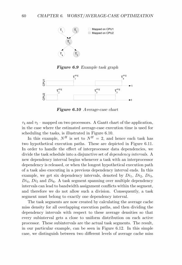
60 CHAPTER 6. WORST/AVERAGE-CASE OPTIMIZATION
τ1
τ2
τ3
τ4
τ5
Mapped on CPU1Mapped on CPU2
Figure 6.9 Example task graph
CPU1
CPU2
t
t
τ1avg τ
4avg
τ2avg avgτ
3avgτ5
Figure 6.10 Average-case chart
τ4 and τ5 – mapped on two processors. A Gantt chart of the application,in the case where the estimated average-case execution time is used forscheduling the tasks, is illustrated in Figure 6.10.
In this example, NH is set to NH = 2, and hence each task hastwo hypothetical execution paths. These are depicted in Figure 6.11.In order to handle the effect of interprocessor data dependencies, wedivide the task schedule into a disjunctive set of dependency intervals. Anew dependency interval begins whenever a task with an interprocessordependency is released, or when the longest hypothetical execution pathof a task also executing in a previous dependency interval ends. In thisexample, we get six dependency intervals, denoted by Di1, Di2, Di3,Di4, Di5 and Di6. A task segment spanning over multiple dependencyintervals can lead to bandwidth assignment conflicts within the segment,and therefore we do not allow such a division. Consequently, a tasksegment must belong to exactly one dependency interval.
The task segments are now created by calculating the average cachemiss density for all overlapping execution paths, and then dividing thedependency intervals with respect to these average densities so thatevery subinterval gets a close to uniform distribution on each activeprocessor. These subintervals are the actual task segments. The result,in our particular example, can be seen in Figure 6.12. In this simplecase, we distinguish between two different levels of average cache miss

6.4. BUS ACCESS OPTIMIZATION FOR ACGD AND WCGD 61
CPU1
CPU2
t
t
τ11 τ
1τ41 τ
422
τ21 τ
22 τ
31 τ
32 τ
51 τ
52
Di1 Di2 Di3 Di5 Di6Di4
Figure 6.11 Average-case chart with corresponding executionpaths
CP
U1
CP
U2
t
t
τ11 τ
1τ41 τ
422
τ21 τ
22 τ
31 τ
32 τ
51 τ
52
i1 i8 i13i2 i3 i4 i5 i6 i7 i9 i10 i11 i12 i14 i15 i16
Low cache miss density High cache miss density
Figure 6.12 Average-case chart with density regions
density. Areas with white color represent regions with low cache missdensity, whereas the gray intervals represent high density regions. Inthis case we get 16 task segments, i1-i16. Dependency interval Di1, forinstance, is divided into task segments i1-i6.
What we, initially, would like to do is to identify the areas of thebus schedule, represented by task segments and bus segments, for whichmodifications can result in the most beneficial change of average-caseglobal delay. In order to perform this identification, we start with aninvestigation of how the bus bandwidth is distributed to the task seg-ments and bus segments, in the average case.
6.4.2 Bus Bandwidth Distribution Analysis
Based on the information from the average-case execution time analysis,for each task segment Ωi ∈ Ξ and bus segment ωj ∈ B, we want todetermine the following:
1. The desired bus bandwidth, that, when given to this particularinterval of the bus schedule, minimizes the global delay in the aver-

62 CHAPTER 6. WORST/AVERAGE-CASE OPTIMIZATION
age case. For a specific task segment Ωi ∈ Ξ, this bandwidth is de-noted PΩi and is a vector of n elements, PΩi = pΩi(1), . . . , pΩi(n),where n is the number of processors in the system and each ele-ment represents the desired bandwidth for the corresponding pro-cessor. Similarly, Pωj = pωj (1), . . . , pωj (n) is the correspondingvector for a bus segment ωj ∈ B. The bandwidth is representedas the fraction of the total bus bandwidth, thus satisfying:∑
k
pΩi(k) = 1,∑k
pωj (k) = 1
Detailed descriptions for how to perform these calculations can befound in Appendix A.1.1.
2. The bandwidth currently given to each processor during the spe-cific interval Ωi ∈ Ξ and ωj ∈ B, represented by the vectors
PbusΩi = pbusΩi
(1), . . . , pbusΩi(n) and P
busωj = pbusωj (1), . . . , pbusωj (n) re-
spectively. Just as for the desired bandwidth, the elements arerepresenting fractions of the total bandwidth, therefore summingup to one. Appendix A.1.2 describes how these two vectors arecalculated.
For a specific task segment Ωk ∈ Ξ, let αΩk ∈ [1..n] ⊆ Z, wheren is the number of processors, denote the processor on which the taskon the critical path, with respect to the average-case task schedule, isexecuted during that particular time interval. Let us define the scalarp∆
Ωk, for a task segment Ωk ∈ Ξ, as the difference between the desired
task bandwidth and the provided bus bandwidth for processor αΩk .That is, p∆
Ωk= pΩk(αΩk)− pbusΩk
(αΩk).Since many task segments can overlap a bus segment, several differ-
ent processors can execute tasks that are on the (same) critical pathduring the particular time interval represented by the bus segment.Hence, let Aωk be the set of processors αωk that are running tasks onthe critical path during the interval represented by bus segment ωk ∈ B.We then define p∆
ωkas:
p∆ωk
= max( ⋃αi∈Aωk
(pωk(αi)− pbusωk
(αi)))
(6.1)
A high p∆Ωi
for a task segment Ωi ∈ Ξ or p∆ωk
for a bus segmentωj ∈ B means that the corresponding interval of the bus schedule has

6.4. BUS ACCESS OPTIMIZATION FOR ACGD AND WCGD 63
room for improvement with respect to the average-case global delay.Therefore, time intervals with a high corresponding p∆
x , x ∈ (Ξ∪B) areinteresting from an optimization point of view, whereas intervals witha low p∆
x , x ∈ (Ξ ∪ B) do not need further investigation. We can nowlimit the search space by just looking at parts of the bus schedule witha corresponding p∆
x , x ∈ (Ξ ∪B) exceeding a specified threshold.
If we wanted to just optimize for the average case, we would start bymodifying the region represented by the segment (task or bus) with thehighest p∆
x , x ∈ (Ξ∪B). However, a large decrease in average-case globaldelay is not necessarily good, if that makes the WCGD increase too big.When deciding which region of the bus schedule to improve, one mustalso take into account the effect on the worst-case global delay. In fact,what we want to improve is the ratio between average-case improvementand worst-case extension, with respect to the global delay. In order forour optimization algorithm to decide how good a bus schedule is forboth the ACGD and WCGD, a cost function is specified in the nextsection.
6.4.3 Cost Function
We denote with length(s) the length of schedule s. Let sworstold and
savgold be worst-case and average-case schedules, for the same applica-
tion, generated with respect to a bus schedule Bold. After creating anew bus schedule Bnew, by modifying a suitable interval of Bold, weobtain updated task schedules sworst
new and savgnew. If an improvement was
made, the task schedules will satisfy length(savgnew) < length(savg
old ) andlength(sworst
new ) > length(sworstold )2 (since the WCGD is expected to grow).
If the bus schedule Bnew does not lead to an improvement with re-spect to the ACGD, it is discarded and not considered further by theoptimization algorithm. Provided that the new bus schedule Bnew ac-tually results in an improvement, a good measure of how good the busmodification is can be given by the ratio:
qsworstnew ,savg
new,sworstold ,savg
old=
length(savgold )− length(savg
new)
length(sworstnew )− length(sworst
old )(6.2)
2For the special case when length(sworstnew ) <= length(sworst
old ), the ratio in Equation6.2 is set to ∞

64 CHAPTER 6. WORST/AVERAGE-CASE OPTIMIZATION
Consequently, a suitable cost function for our optimization algorithmcan be expressed as:
C(sworstnew , savg
new, sworstold , savg
old ) = −qsworstnew ,savg
new,sworstold ,savg
old(6.3)
With respect to this cost function, we can now evaluate a set of busschedule candidates and choose the best one.
6.4.4 Bus Schedule Optimization
We create a new bus schedule candidate Bk′ from bus schedule Bk(taken as input parameter on line 4 in Figure 6.8) by modifying thepart of Bk corresponding to the time interval represented by a task seg-ment Ωi ∈ Ξ or bus segment ωj ∈ B. To calculate the cost of Bk′ , wemust compute the schedules sworstk′ and savgk′ . This is done by invokingthe execution time analysis framework twice, for the entire applica-tion, and that is relatively costly from a computation-time perspective.Therefore, as stated previously, the solution is to limit the search spaceand thus only generate candidates that are likely to perform good. Itcan be assumed that improving areas corresponding to segments witha low p∆
Ωior p∆
ωj , for Ωi ∈ Ξ and ωj ∈ B respectively, will not lead tothe best results, since the room for average-case global delay improve-ments is small. Therefore, we define Ξ′ as the set of the t task segmentsΩi ∈ Ξ which have the greatest corresponding p∆
Ωivalues. Similarly,
B′ is defined as the set of b bus segments ωj ∈ B with the greatestcorresponding p∆
ωi . The t+ b segments in Ξ′∪B′ are selected for furtherinvestigation. High t and b values, set by the designer, allow the algo-rithm to evaluate more bus schedule candidates, but at the expense ofcomputation time.
For each segment in Ξ′∪B′, we want to generate several bus schedulecandidates and evaluate them with respect to the cost function definedin Equation 6.3. When no more bus schedule candidates are left toevaluate for any segment in Ξ′ ∪ B′, the candidate associated with thelowest cost is kept and returned as bus schedule Bk+1 (line 4 in Figure6.8).
The first bus schedule candidate Bk′0 for a specific segment in Ξ′∪B′is generated by inserting a new bus segment into the previously gener-ated bus schedule Bk. This new bus segment is constituted by a TDMAround r, generated so that the bus bandwidth during the correspond-ing interval is assigned according to the desired bus bandwidth PΩi orPωj , depending on if the segment in Ξ′ ∪B′ being investigated is a task

6.5. EXPERIMENTAL RESULTS 65
segment Ωi ∈ Ξ′ or a bus segment ωj ∈ B′. With respect to the busschedule candidate Bk′0 , the schedules sworst
k′0and savg
k′0are generated and
Bk′0 is then evaluated according to the cost function in Equation 6.3.To create the next bus schedule candidate Bk′i (where now, in this case,i = 1) for the same segment, round r is modified according to the out-come of the execution time analysis, using the hill climbing optimizationtechnique to adjust the bandwidth distribution. Other modifications,such as slot order permutations, can also be carried out depending onthe restrictions imposed on TDMA complexity. The procedure of im-proving round r – each improvement resulting in a new bus schedulecandidate – is repeated a specified number of times or until no furtherimprovements are found, and then the next segment in Ξ′ ∪B′ is inves-tigated. The best bus schedule candidate Bk′ is then chosen as the newbus schedule Bk+1 for the application, and the function returns. Theimprove function is summarized in Figure 6.13.
Note that adding new bus segments will increase the complexity ofthe bus schedule. Since the memory on the bus arbiter is limited, theremight be a limit for how many bus segments we can allow. Once thismaximum number of bus segments is reached, we cannot increase thenumber of segments of the bus schedule without first deleting at leastone, already existing, bus segment. Therefore, immediately after in-serting the new bus segment, resulting in the bus schedule candidateBk′0 , and before making any improvements to the corresponding roundr constituting it, we evaluate the effect of merging every pair of consec-utive bus segments in the bus schedule using the ACGD and WCGDanalyses and computing the resulting cost. The best merge is then kept,and we continue by generating more bus schedule candidates Bk′i (bytrying to improve r, as usual). Note that this is only a problem whenimproving the bus schedule with respect to task segments Ωi ∈ Ξ′, sinceimproving with respect to bus segments ωj ∈ B′ does not increase thebus schedule complexity.
6.5 Experimental Results
We have evaluated our framework using an extensive set of generated Cprograms. The programs were constructed with respect to randomizedtask graphs consisting of between 20 and 200 tasks, mapped on 2 to 8processors. The individual tasks were generated according to controlflow graphs corresponding to programs for commonly used computa-

66 CHAPTER 6. WORST/AVERAGE-CASE OPTIMIZATION
01: Perform an average-case execution time analysis.
02: Divide the resulting task schedule into a set of
task segments Ξ.03: Calculate current and desired bus bandwidth,
PΩiand Pωj , with respect to the ACGD only, for
each task segment and bus segment.
04: Calculate Ξ′ and B′.05: For each element in Ξ′ ∪B′, generate a set of
bus schedule candidates and evaluate them
according to the cost function in Equation 6.3.
06: Return the candidate that generates the lowest cost,
while keeping the WCGD below WCGDmax.
Figure 6.13 The improve function
tions such as sorting, searching, matrix multiplications and DSP pro-cessing. In total, 8000 applications were generated and evaluated. Tocalculate the memory access histograms, as described in Section 6.2,1000 executions were carried out for each task.
As hardware platform, we have used the MPARM multiprocessorcycle-accurate simulator from Bologna University [15], configured ac-cording to the model in Section 2.1, using 8 ARM7 cores running at200 MHz. An AMBA AHB-compliant bus arbiter, enforcing the busmodel in Section 2.3, was implemented and incorporated into the sim-ulation framework. The bus speed was set to 100 MHz, resulting ina memory access taking 13 CPU clock cycles to serve. In order to re-strict the amount of memory on the controller, we imposed the followingrestrictions on TDMA round complexity:
1. A processor can own at most one slot in a TDMA round.
2. The slot order is fixed, and cannot be changed during the opti-mization procedure.
The values of t and b, described in Section 6.4.4, were set to 100 and 50,respectively. We also limited the total number of bus segments allowedin the bus schedule to 1000.
Using the approach described in Chapters 3 and 5, for each of theapplications, we started by generating a bus schedule minimizing theworst-case global delay, completely ignoring the average case. Let us de-note this initial, minimized, worst-case global delay by WCGD0, and letACGD0 be the ACGD calculated with respect to the same bus schedule.

6.5. EXPERIMENTAL RESULTS 67
2 3 4 5 6 7 80
2
4
6
8
10
12
14
16
1%5%10%
Number of Processors
ACG
D Im
prov
emen
t (%
)WCGD Extension:
Figure 6.14 Relative ACGD improvement
The bus schedule, optimized for the worst case, and the correspondingworst-case task schedule were then sent as input parameters to the al-gorithm outlined in Figure 6.8, together with the generated memoryaccess histograms for each task in the application task graph. A maxi-mum allowed WCGD was also supplied.
We now investigated how much the ACGD can be decreased, given amaximum allowed increment (with respect to WCGD0) of the resultingWCGD. For all applications, we performed the optimization procedurethree times, allowing WCGD increments of 1%, 5% and 10% respec-tively. For each of these allowed increments, a corresponding averageACGD improvement was calculated. The result is presented in Fig-ure 6.14. For instance, for two processors, accepting an 1% extensionwith respect to WCGD0 leads to an average ACGD improvement of13.2%. Accepting a greater WCGD increment naturally results in amore substantial ACGD reduction. It can be observed that using alower number of processors allows for a higher ACGD decrement, withrespect to ACGD0. This is explained by the fact that fewer competingprocessors leave more room for tailoring the bus schedule for a specificprocessor, allowing for a more flexible design.
In a second experiment, we investigated how optimizing for theACGD, without considering the WCGD at all, affects the latter. Theidea is to show that optimizing only for the ACGD leads to unreasonablyhigh worst-case global delays, compared to when optimizing for both.For this second experiment, we used the very same generated test ex-amples as in the first experiment, allowing for direct comparisons with

68 CHAPTER 6. WORST/AVERAGE-CASE OPTIMIZATION
2 3 4 5 6 7 80
5
10
15
20
25
WCGD ExtensionACGD Improvement
Number of Processors
Glo
bal D
elay
Cha
nge
(%)
Figure 6.15 Relative ACGD improvement and WCGD exten-sion
the already calculated WCET0 and ACET0. Initially, an algorithm foroptimizing the bus schedule, taking into account only the ACGD, wasapplied to the test applications, and then the WCGD was calculatedwith respect to that bus schedule. Let us denote the resulting ACGDand WCGD by ACGD′0 and WCGD′0 respectively. In Figure 6.15, wehave plotted the relative average extension of WCGD′0 compared toWCGD0, and the average reduction of ACGD′0 compared to ACGD0.As can be seen, not taking the WCGD into consideration when optimiz-ing the bus schedule leads to higher worst-case global delays, whereasthe corresponding ACGD improvement is only slightly better than whenalso optimizing for the WCGD and accepting a WCGD increase of 10%.For instance, for a 5 processor application, the WCGD extension com-pared to the optimal case (WCGD0) is 15% whereas the improvement ofthe ACGD relative ACGD0 is 6.0%. By looking in Figure 6.14, we cansee that when optimizing for both ACGD and WCGD simultaneously,for 5 processors we can obtain a 5.5% (instead of 6%) improvement withonly a 10% (compared to 15%) degradation of the WCGD.
All experiments were executed on a dual core Pentium 4 processorrunning at 2.8 GHz. The time to process one application ranged from10 minutes to 4 hours, depending on the application complexity.

7
Conclusions
In this thesis, we have presented an approach to achieve time-predictabilityfor real-time applications running on modern multiprocessor systems-on-chip, taking into consideration potential memory access conflicts be-tween concurrent tasks. In particular, we have focused on the issue ofbus access optimization. Efficient algorithms for minimizing the worst-case global delay have been proposed, making sure that the price to payfor predictability, in terms of time, becomes as small as possible.
We have also presented an entirely new, within the domain of real-time systems, concept of optimizing for the average-case global delaywhile keeping the WCGD as small as possible. The proposed algorithmsshow that this dual approach is more efficient than optimizing only foreither the worst-case or the average-case.
All algorithms were validated by an extensive sets of experiments.
69

70 References

Bibliography
[1] A. Andrei, P. Eles, Z. Peng, and J. Rosen, “Predictable Implemen-tation of Real-Time Applications on Multiprocessor Systems-on-Chip,” in VLSI Conference, 2008.
[2] D. Bertozzi, A. Guerri, M. Milano, F. Poletti, and M. Rug-giero, “Communication-Aware Allocation and Scheduling Frame-work for Stream-Oriented Multi-Processor Systems-on-Chip,” inDATE, 2006, pp. 3–8.
[3] C.-F. Neikter, “Cache Prediction and Execution Time Analysis onReal-Time MPSoC,” 2008, Master Thesis, LIU-IDA/LITH-EX-A–08/046–SE.
[4] J. M. Calandrino, J. H. Anderson, and D. P. Baumberger, “AHybrid Real-Time Scheduling Approach for Large-Scale MulticorePlatforms,” in ECRTS, 2007.
[5] S. A. Edwards and E. A. Lee, “The Case for the PrecisionTimed (PRET) Machine,” EECS Department Technical Report No.UCB/EECS-2006-149, University of California, Berkeley, 2006.
71

72 References
[6] H. Falk, “WCET-aware Register Allocation based on Graph Col-oring,” in DAC, 2009.
[7] H. Falk and J. C. Kleinsorge, “Optimal Static WCET-awareScratchpad Allocation of Program Code,” in DAC, 2009.
[8] K. Goossens, J. Dielissen, and A. Radulescu, “AEthereal Networkon Chip: Concepts, Architectures, and Implementations,” IEEEDesign & Test of Computers, vol. 2/3, pp. 115–127, 2005.
[9] M. Joseph and P. Pandya, “Finding Response Times in a Real-Time System,” The Computer Journal, vol. 29, 1986.
[10] E. C. Jr and R. Graham, “Optimal Scheduling for Two-ProcessorSystems,” Acta Inform., vol. 1, pp. 200–213, 1972.
[11] I. A. Khatib, D. Bertozzi, F. Poletti, L. Benini, and et al., “A Mul-tiprocessor Systems-on-Chip for Real-Time Biomedical Monitoringand Analysis: Architectural Design Space Exploration,” in DAC,2006, pp. 125–131.
[12] B. Lickly, I. Liu, S. Kim, H. D. Patel, S. A. Edwards, and E. A.Lee, “Predictable Programming on a Precision Timed Architec-ture,” EECS Department Technical Report No. UCB/EECS-2008-40, University of California, Berkeley, 2008.
[13] T. Lundqvist and P. Stenstrom, “Timing Anomalies in Dynam-ically Scheduled Microprocessors,” in The 20th IEEE Real-TimeSystems Symposium (RTSS), 1999, pp. 12–21.
[14] M. Lv, N. Guan, W. Yi, and G. Yu, “Combining Abstract Interpre-tation with Model Checking for Timing Analysis of Multicore Soft-ware,” in The 31st IEEE Real-Time Systems Symposium (RTSS),2010.
[15] MPARM homepage,“http://www-micrel.deis.unibo.it/sitonew/research/mparm.html”.
[16] F. Nemati, M. Behnam, and T. Nolte, “Independently-Developed Real-Time Systems on Multi-Cores with Shared Re-sources,” in 23rd EUROMICRO Conference on Real-Time Systems(ECRTS’11), July 2011.

References 73
[17] M. Paolieri, E. Quinones, F. J. Cazorla, G. Bernat, and M. Valero,“Hardware Support for WCET Analysis of Hard Real-Time Mul-ticore Systems,” in ISCA, 2009, pp. 57–68.
[18] S. Pasricha, N. Dutt, and M. Ben-Romdhane, “Fast Explo-ration of Bus-based On-chip Communication Architectures,” inCODES+ISSS, 2004, pp. 242–247.
[19] R. Pellizzoni and M. Caccamo, “Impact of Peripheral-Processor In-terference on WCET Analysis of Real-Time Embedded Systems,”IEEE Transactions on Computers, vol. 59, no. 3, pp. 400–415,2010.
[20] P. Pop, P. Eles, Z. Peng, and T. Pop, “Analysis and Optimizationof Distributed Real-Time Embedded Systems,” ACM Transactionson Design Automation of Electronic Systems, vol. Vol. 11, pp. 593–625, 2006.
[21] P. Puschner and A. Burns, “A Review of Worst-Case Execution-Time Analysis,” Real-Time Systems, vol. 2/3, pp. 115–127, 2000.
[22] J. Reineke, B.Wachter, S. Thesing, R.Wilhelm, I. Polian,J. Eisinger, and B. Becker, “A Definition and Classification of Tim-ing Anomalies,” in International Workshop on WCET Analysis,2006, pp. 23–28.
[23] J. Rosen, A. Andrei, P. Eles, and Z. Peng, “Bus Access Optimiza-tion for Predictable Implementation of Real-Time Applications onMultiprocessor Systems-on-Chip,” in The 28th IEEE Real-TimeSystems Symposium (RTSS), 2007, pp. 49–60.
[24] J. Rosen, P. Eles, Z. Peng, and A. Andrei, “Predictable Worst-CaseExecution Time Analysis for Multiprocessor Systems-on-Chip,” inThe 6th International Symposium on Electronic Design, Test andApplications (DELTA), 2011.
[25] J. Rosen, C.-F. Neikter, P. Eles, Z. Peng, P. Burgio, and L. Benini,“Bus Access Design for Combined Worst and Average Case Execu-tion Time Optimization of Predictable Real-Time Applications onMultiprocessor Systems-on-Chip,” in The 17th IEEE Real-Timeand Embedded Technology and Applications Symposium (RTAS),2011.

74 References
[26] E. Salminen, V. Lahtinen, K. Kuusilinna, and T. Hamalainen,“Overview of Bus-Based System-on-Chip Interconnections,” in IS-CAS, 2002, pp. 372–375.
[27] S. Schliecker, M. Ivers, and R. Ernst, “Integrated Analysis ofCommunicating Tasks in MPSoCs,” in The International Con-ference on Hardware/Software Codesign and System Synthesis(CODES+ISSS), 2006, pp. 288–293.
[28] S. Schliecker, M. Negrean, and R. Ernst, “Bounding the SharedResource Load for the Performance Analysis of MultiprocessorSystems,” in Proc. of Design, Automation, and Test in Europe(DATE), Dresden, Germany, 2010.
[29] S. Schliecker, M. Negrean, G. Nicolescu, P. Paulin, and R. Ernst,“Reliable Performance Analysis of a Multicore MultithreadedSystem-On-Chip,” in The International Conference on Hard-ware/Software Codesign and System Synthesis (CODES+ISSS),2008.
[30] M. Schoeberl and P. Puschner, “Is Chip-Multiprocessing the End ofReal-Time Scheduling?” in 9th International Workshop on Worst-Case Execution Time (WCET) Analysis, 2009.
[31] A. Schranzhofer, J.-J. Chen, and L. Thiele, “Timing Analysis forTDMA Arbitration in Resource Sharing Systems,” in 16th IEEEReal-Time and Embedded Technology and Applications Symposium(RTAS), 2010, pp. 215–224.
[32] L. Thiele and R. Wilhelm, “Design for Timing Predictability,”Real-Time Systems, vol. 28, no. 2/3, pp. 157–177, 2004.
[33] R. Wilhelm, J. Engblom, A. Ermedahl, N. Holsti, S. Thesing,D. Whalley, G. Bernat, C. Ferdinand, R. Heckmann, T. Mitra,F. Mueller, I. Puaut, P. Puschner, J. Staschulat, , and P. Sten-strom, “The Worst-Case Execution Time Problem – Overview ofMethods and Survey of Tools,” ACM Transactions on EmbeddedComputing Systems (TECS), vol. 7, no. 3, 2008.
[34] R. Wilhelm, D. Grund, J. Reineke, M. Schlickling, M. Pister, andC. Ferdinand, “Memory Hierarchies, Pipelines, and Buses for Fu-ture Architectures in Time-Critical Embedded Systems,” IEEETransactions on CAD of Integrated Circuits and Systems, 2009.

References 75
[35] S. Williams, A. Waterman, and D. Patterson, “Roofline: An In-sightful Visual Performance Model for Multicore Architectures,”Communications of the ACM, vol. 52, no. 4, 2009.
[36] W. Wolf, Computers as Components: Principles of EmbeddedComputing System Design. Morgan Kaufman Publishers, 2005.
[37] J. Yan and W. Zhang, “WCET Analysis for Multi-Core Processorswith Shared L2 Instruction Caches,” in 14th IEEE Real-Time andEmbedded Technology and Applications Symposium (RTAS), 2008,pp. 80–89.

76 References

A
Bus Bandwidth Calculations
A.1 Bus Bandwidth Calculations
This section presents the theoretical foundation for the bus bandwidthcalculations needed by the optimization algorithm in Section 6.3. Wedemonstrate how to calculate the desired bus bandwidth that theoret-ically will result in the lowest possible average-case global delay. Thisis done for both task segments and bus segments, as defined in Section6.3. Furthermore, we show how to calculate the current bus bandwidththat is actually being distributed to the active processors. While thisprocedure is trivial for bus segments, it requires more computations fortask segments.
A.1.1 Calculation of the Desired Bus Bandwidth
We will now describe how to calculate the desired bandwidth PΩi fora task segment Ωi ∈ Ξ, or Pωi for a bus segment ωi ∈ B, as requiredby the algorithm in Section 6.3. Since a bus segment can be seen as aparticular variant of a task segment, we will only talk about the latter
77

78 APPENDIX A. BUS BANDWIDTH CALCULATIONS
in this section.
The overall idea is the same as for the approach used in Chapter5, where the the initial slot sizes of a TDMA bus schedule are deter-mined by formulating a set of inequalities. In that section, we calculatethe bandwidth distribution that theoretically minimizes the worst-caseglobal delay. Now, on the other hand, we want to do the same, butwith respect to the ACGD instead. While these are similar proceduressharing many computation steps, there are several significant differencesbetween them.
First, it is assumed that an average-case execution time analysis hasbeen performed with respect to a bus schedule, partly or fully tailoredfor the worst case. The desired bus bandwidth for a specific part of thisbus schedule is, in this context, the distribution of bandwidth that willreduce the average-case global delay as much as possible.
Let τ si be the first task after τi ∈ Tj that is scheduled on the sameprocessor. Furthermore, let D1
i be the set of all tasks τj ∈ G(Π,Γ)which task τ si depends directly on in the task graph G(Π,Γ). Now, Di
is defined as the set τi∪D1i . This means that task τ si will be released
only when all tasks in Di have finished executing.
Now, for a task segment Ωk ∈ Ξ, let us define the following functions:
• fok (τ ji ) is defined as the number of time units of the execution path
τ ji (of task τi) that executes during the time interval representedby Ωk ∈ Ξ.
• fmk (τ ji ) is defined as the number of cache misses on the execu-
tion path τ ji (of task τi) that is issued during the time intervalrepresented by Ωk ∈ Ξ.
• f sk(τ
ji ) is defined as the number of time units execution path τ ji (of
task τi) spends executing code during the time interval representedby Ωk ∈ Ξ, excluding transfer times.
We also define the following functions, not specific to a particulartask segment:
• fp(τ ji ) is defined as the length, in time units, of the execution
path τ ji (of task τi).
• u(τi) is defined as the processor number that task τi is executingon.

A.1. BUS BANDWIDTH CALCULATIONS 79
Remember that the desired bandwidth, represented as the fraction ofthe total bandwidth, for a task τi ∈ Tj running on processor β duringthe time interval represented by Ωj is defined as pΩj (β). Let us, forconvenience, denote this fraction as pi. If a is defined as the time ittakes for the bus to immediately transfer a cache miss, the averagewaiting time can then be modeled in terms of the desired bandwidth asfollows:
di =1
pia (A.1)
Let us define Gβ as the set of tasks τi ∈ G(Π,Γ) executing on pro-cessor β, and let N be the number of processors. The number of hypo-thetical paths is denoted by NH . We can now estimate the average-caseglobal delay, as a function of the bus bandwidth given during the tasksegment Ωk ∈ Ξ, by the following formula:
maxβ=0..N
∑τq∈Gβ
maxτi∈Dq
∑j=1..NH fp(τ ji )− fo
k (τ ji ) + fmk (τ ji )du(τi) + f s
k(τ ji )
NH
(A.2)
We want to calculate the bandwidth distribution resulting in theshortest global delay. This can be done by solving - with respect tothe bandwidth distribution p1, p2, . . ., pN and the global delay t - thefollowing system of inequalities:
∑τq∈G1
maxτi∈Dq
∑j=1..NH fp(τ ji )− fo
k (τ ji ) + fmk (τ ji ) a
pu(τi)+ f s
k(τ ji )
NH≤ t
∑τq∈G2
maxτi∈Dq
∑j=1..NH fp(τ ji )− fo
k (τ ji ) + fmk (τ ji ) a
pu(τi)+ f s
k(τ ji )
NH≤ t
...∑τq∈GN
maxτi∈Dq
∑j=1..NH fp(τ ji )− fo
k (τ ji ) + fmk (τ ji ) a
pu(τi)+ f s
k(τ ji )
NH≤ t
p1 + p2 + · · ·+ pn = 1
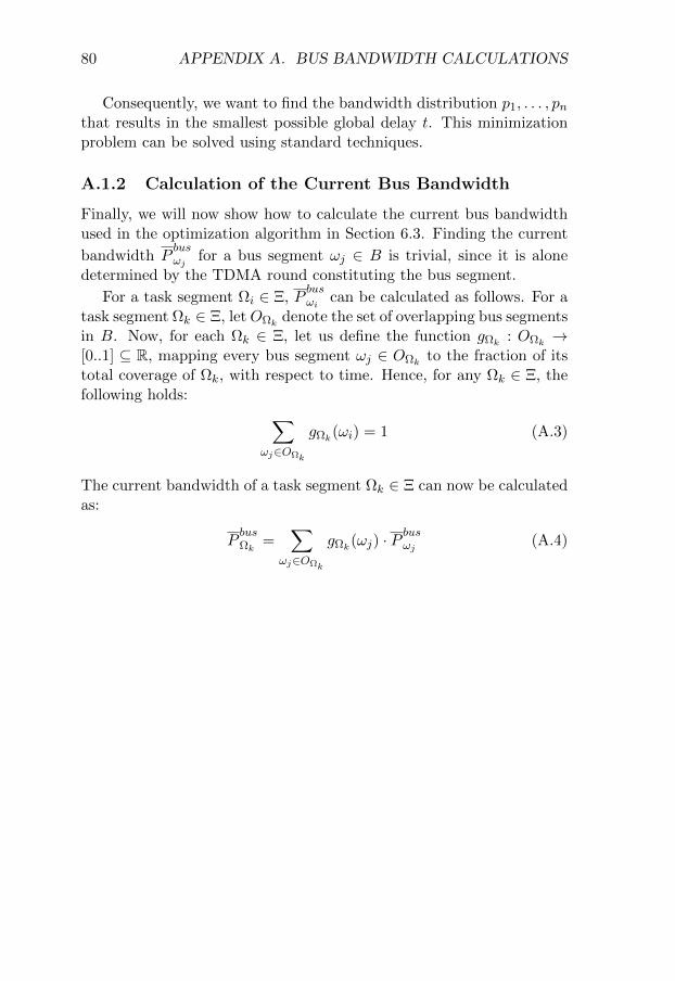
80 APPENDIX A. BUS BANDWIDTH CALCULATIONS
Consequently, we want to find the bandwidth distribution p1, . . . , pnthat results in the smallest possible global delay t. This minimizationproblem can be solved using standard techniques.
A.1.2 Calculation of the Current Bus Bandwidth
Finally, we will now show how to calculate the current bus bandwidthused in the optimization algorithm in Section 6.3. Finding the current
bandwidth Pbusωj for a bus segment ωj ∈ B is trivial, since it is alone
determined by the TDMA round constituting the bus segment.
For a task segment Ωi ∈ Ξ, Pbusωi can be calculated as follows. For a
task segment Ωk ∈ Ξ, let OΩk denote the set of overlapping bus segmentsin B. Now, for each Ωk ∈ Ξ, let us define the function gΩk : OΩk →[0..1] ⊆ R, mapping every bus segment ωj ∈ OΩk to the fraction of itstotal coverage of Ωk, with respect to time. Hence, for any Ωk ∈ Ξ, thefollowing holds: ∑
ωj∈OΩk
gΩk(ωi) = 1 (A.3)
The current bandwidth of a task segment Ωk ∈ Ξ can now be calculatedas:
PbusΩk
=∑
ωj∈OΩk
gΩk(ωj) · Pbusωj (A.4)

LINKÖPINGS UNIVERSITET
Rapporttyp
Report category
Licentiatavhandling
Examensarbete
C-uppsats
D-uppsats
Övrig rapport
Språk Language
Svenska/Swedish
Engelska/English
Titel Title
Författare Author
Sammanfattning Abstract
ISBN
ISRN
Serietitel och serienummer ISSN Title of series, numbering
Linköping Studies in Science and Technology
Thesis No. 1503
Nyckelord Keywords
Datum Date
URL för elektronisk version
X
X
2011-09-30
Avdelning, institution Division, department
Institutionen för datavetenskap
Department of Computer
and Information Science
http://urn.kb.se/resolve?urn=urn:nbn:se:liu:diva-70138
Predictable Real-Time Applications on Multiprocessor Systems-on-Chip
Jakob Rosén
Being predictable with respect to time is, by definition, a fundamental requirement for any real-time system. Modern
multiprocessor systems impose a challenge in this context, due to resource sharing conflicts causing memory
transfers to become unpredictable. In this thesis, we present a framework for achieving predictability for real-time
applications running on multiprocessor system-on-chip platforms. Using a TDMA bus, worst-case execution time
analysis and scheduling are done simultaneously. Since the worst-case execution times are directly dependent on the
bus schedule, bus access design is of special importance. Therefore, we provide an efficient algorithm for generating
bus schedules, resulting in a minimized worst-case global delay.
We also present a new approach considering the average-case execution time in a predictable context. Optimization
techniques for improving the average-case execution time of tasks, for which predictability with respect to time is not
required, have been investigated for a long time in many different contexts. However, this has traditionally been done
without paying attention to the worst-case execution time. For predictable real-time applications, on the other hand,
the focus has been solely on worst-case execution time optimization, ignoring how this affects the execution time in
the average case. In this thesis, we show that having a good average-case global delay can be important also for real-
time applications, for which predictability is required. Furthermore, for real-time applications running on
multiprocessor systems-on-chip, we present a technique for optimizing for the average case and the worst case
simultaneously, allowing for a good average case execution time while still keeping the worst case as small as
possible. The proposed solutions in this thesis have been validated by extensive experiments. The results
demonstrate the efficiency and importance of the presented techniques.
Computer Systems, Embedded Systems, Real-Time Systems, Predictability, Multiprocessor Systems
978-91-7393-090-1
0280-7971
LIU-TEK-LIC-2011:42


Department of Computer and Information Science
Linköpings universitet
Licentiate Theses
Linköpings Studies in Science and Technology
Faculty of Arts and Sciences
No 17 Vojin Plavsic: Interleaved Processing of Non-Numerical Data Stored on a Cyclic Memory. (Available at: FOA,
Box 1165, S-581 11 Linköping, Sweden. FOA Report B30062E)
No 28 Arne Jönsson, Mikael Patel: An Interactive Flowcharting Technique for Communicating and Realizing Al-
gorithms, 1984.
No 29 Johnny Eckerland: Retargeting of an Incremental Code Generator, 1984.
No 48 Henrik Nordin: On the Use of Typical Cases for Knowledge-Based Consultation and Teaching, 1985.
No 52 Zebo Peng: Steps Towards the Formalization of Designing VLSI Systems, 1985.
No 60 Johan Fagerström: Simulation and Evaluation of Architecture based on Asynchronous Processes, 1985.
No 71 Jalal Maleki: ICONStraint, A Dependency Directed Constraint Maintenance System, 1987.
No 72 Tony Larsson: On the Specification and Verification of VLSI Systems, 1986.
No 73 Ola Strömfors: A Structure Editor for Documents and Programs, 1986.
No 74 Christos Levcopoulos: New Results about the Approximation Behavior of the Greedy Triangulation, 1986.
No 104 Shamsul I. Chowdhury: Statistical Expert Systems - a Special Application Area for Knowledge-Based Computer
Methodology, 1987.
No 108 Rober Bilos: Incremental Scanning and Token-Based Editing, 1987.
No 111 Hans Block: SPORT-SORT Sorting Algorithms and Sport Tournaments, 1987.
No 113 Ralph Rönnquist: Network and Lattice Based Approaches to the Representation of Knowledge, 1987.
No 118 Mariam Kamkar, Nahid Shahmehri: Affect-Chaining in Program Flow Analysis Applied to Queries of Pro-
grams, 1987.
No 126 Dan Strömberg: Transfer and Distribution of Application Programs, 1987.
No 127 Kristian Sandahl: Case Studies in Knowledge Acquisition, Migration and User Acceptance of Expert Systems,
1987.
No 139 Christer Bäckström: Reasoning about Interdependent Actions, 1988.
No 140 Mats Wirén: On Control Strategies and Incrementality in Unification-Based Chart Parsing, 1988.
No 146 Johan Hultman: A Software System for Defining and Controlling Actions in a Mechanical System, 1988.
No 150 Tim Hansen: Diagnosing Faults using Knowledge about Malfunctioning Behavior, 1988.
No 165 Jonas Löwgren: Supporting Design and Management of Expert System User Interfaces, 1989.
No 166 Ola Petersson: On Adaptive Sorting in Sequential and Parallel Models, 1989.
No 174 Yngve Larsson: Dynamic Configuration in a Distributed Environment, 1989.
No 177 Peter Åberg: Design of a Multiple View Presentation and Interaction Manager, 1989.
No 181 Henrik Eriksson: A Study in Domain-Oriented Tool Support for Knowledge Acquisition, 1989.
No 184 Ivan Rankin: The Deep Generation of Text in Expert Critiquing Systems, 1989.
No 187 Simin Nadjm-Tehrani: Contributions to the Declarative Approach to Debugging Prolog Programs, 1989.
No 189 Magnus Merkel: Temporal Information in Natural Language, 1989.
No 196 Ulf Nilsson: A Systematic Approach to Abstract Interpretation of Logic Programs, 1989.
No 197 Staffan Bonnier: Horn Clause Logic with External Procedures: Towards a Theoretical Framework, 1989.
No 203 Christer Hansson: A Prototype System for Logical Reasoning about Time and Action, 1990.
No 212 Björn Fjellborg: An Approach to Extraction of Pipeline Structures for VLSI High-Level Synthesis, 1990.
No 230 Patrick Doherty: A Three-Valued Approach to Non-Monotonic Reasoning, 1990.
No 237 Tomas Sokolnicki: Coaching Partial Plans: An Approach to Knowledge-Based Tutoring, 1990.
No 250 Lars Strömberg: Postmortem Debugging of Distributed Systems, 1990.
No 253 Torbjörn Näslund: SLDFA-Resolution - Computing Answers for Negative Queries, 1990.
No 260 Peter D. Holmes: Using Connectivity Graphs to Support Map-Related Reasoning, 1991.
No 283 Olof Johansson: Improving Implementation of Graphical User Interfaces for Object-Oriented Knowledge- Bases,
1991.
No 298 Rolf G Larsson: Aktivitetsbaserad kalkylering i ett nytt ekonomisystem, 1991.
No 318 Lena Srömbäck: Studies in Extended Unification-Based Formalism for Linguistic Description: An Algorithm for
Feature Structures with Disjunction and a Proposal for Flexible Systems, 1992.
No 319 Mikael Pettersson: DML-A Language and System for the Generation of Efficient Compilers from Denotational
Specification, 1992.
No 326 Andreas Kågedal: Logic Programming with External Procedures: an Implementation, 1992.
No 328 Patrick Lambrix: Aspects of Version Management of Composite Objects, 1992.
No 333 Xinli Gu: Testability Analysis and Improvement in High-Level Synthesis Systems, 1992.
No 335 Torbjörn Näslund: On the Role of Evaluations in Iterative Development of Managerial Support Systems, 1992.
No 348 Ulf Cederling: Industrial Software Development - a Case Study, 1992.
No 352 Magnus Morin: Predictable Cyclic Computations in Autonomous Systems: A Computational Model and Im-
plementation, 1992.
No 371 Mehran Noghabai: Evaluation of Strategic Investments in Information Technology, 1993.
No 378 Mats Larsson: A Transformational Approach to Formal Digital System Design, 1993.

No 380 Johan Ringström: Compiler Generation for Parallel Languages from Denotational Specifications, 1993.
No 381 Michael Jansson: Propagation of Change in an Intelligent Information System, 1993.
No 383 Jonni Harrius: An Architecture and a Knowledge Representation Model for Expert Critiquing Systems, 1993.
No 386 Per Österling: Symbolic Modelling of the Dynamic Environments of Autonomous Agents, 1993.
No 398 Johan Boye: Dependency-based Groudness Analysis of Functional Logic Programs, 1993.
No 402 Lars Degerstedt: Tabulated Resolution for Well Founded Semantics, 1993.
No 406 Anna Moberg: Satellitkontor - en studie av kommunikationsmönster vid arbete på distans, 1993.
No 414 Peter Carlsson: Separation av företagsledning och finansiering - fallstudier av företagsledarutköp ur ett agent-
teoretiskt perspektiv, 1994.
No 417 Camilla Sjöström: Revision och lagreglering - ett historiskt perspektiv, 1994.
No 436 Cecilia Sjöberg: Voices in Design: Argumentation in Participatory Development, 1994.
No 437 Lars Viklund: Contributions to a High-level Programming Environment for a Scientific Computing, 1994.
No 440 Peter Loborg: Error Recovery Support in Manufacturing Control Systems, 1994.
FHS 3/94 Owen Eriksson: Informationssystem med verksamhetskvalitet - utvärdering baserat på ett verksamhetsinriktat och
samskapande perspektiv, 1994.
FHS 4/94 Karin Pettersson: Informationssystemstrukturering, ansvarsfördelning och användarinflytande - En komparativ
studie med utgångspunkt i två informationssystemstrategier, 1994.
No 441 Lars Poignant: Informationsteknologi och företagsetablering - Effekter på produktivitet och region, 1994.
No 446 Gustav Fahl: Object Views of Relational Data in Multidatabase Systems, 1994.
No 450 Henrik Nilsson: A Declarative Approach to Debugging for Lazy Functional Languages, 1994.
No 451 Jonas Lind: Creditor - Firm Relations: an Interdisciplinary Analysis, 1994.
No 452 Martin Sköld: Active Rules based on Object Relational Queries - Efficient Change Monitoring Techniques, 1994.
No 455 Pär Carlshamre: A Collaborative Approach to Usability Engineering: Technical Communicators and System
Developers in Usability-Oriented Systems Development, 1994.
FHS 5/94 Stefan Cronholm: Varför CASE-verktyg i systemutveckling? - En motiv- och konsekvensstudie avseende
arbetssätt och arbetsformer, 1994.
No 462 Mikael Lindvall: A Study of Traceability in Object-Oriented Systems Development, 1994.
No 463 Fredrik Nilsson: Strategi och ekonomisk styrning - En studie av Sandviks förvärv av Bahco Verktyg, 1994.
No 464 Hans Olsén: Collage Induction: Proving Properties of Logic Programs by Program Synthesis, 1994.
No 469 Lars Karlsson: Specification and Synthesis of Plans Using the Features and Fluents Framework, 1995.
No 473 Ulf Söderman: On Conceptual Modelling of Mode Switching Systems, 1995.
No 475 Choong-ho Yi: Reasoning about Concurrent Actions in the Trajectory Semantics, 1995.
No 476 Bo Lagerström: Successiv resultatavräkning av pågående arbeten. - Fallstudier i tre byggföretag, 1995.
No 478 Peter Jonsson: Complexity of State-Variable Planning under Structural Restrictions, 1995.
FHS 7/95 Anders Avdic: Arbetsintegrerad systemutveckling med kalkylprogram, 1995.
No 482 Eva L Ragnemalm: Towards Student Modelling through Collaborative Dialogue with a Learning Companion,
1995.
No 488 Eva Toller: Contributions to Parallel Multiparadigm Languages: Combining Object-Oriented and Rule-Based
Programming, 1995.
No 489 Erik Stoy: A Petri Net Based Unified Representation for Hardware/Software Co-Design, 1995.
No 497 Johan Herber: Environment Support for Building Structured Mathematical Models, 1995.
No 498 Stefan Svenberg: Structure-Driven Derivation of Inter-Lingual Functor-Argument Trees for Multi-Lingual
Generation, 1995.
No 503 Hee-Cheol Kim: Prediction and Postdiction under Uncertainty, 1995.
FHS 8/95 Dan Fristedt: Metoder i användning - mot förbättring av systemutveckling genom situationell metodkunskap och
metodanalys, 1995.
FHS 9/95 Malin Bergvall: Systemförvaltning i praktiken - en kvalitativ studie avseende centrala begrepp, aktiviteter och
ansvarsroller, 1995.
No 513 Joachim Karlsson: Towards a Strategy for Software Requirements Selection, 1995.
No 517 Jakob Axelsson: Schedulability-Driven Partitioning of Heterogeneous Real-Time Systems, 1995.
No 518 Göran Forslund: Toward Cooperative Advice-Giving Systems: The Expert Systems Experience, 1995.
No 522 Jörgen Andersson: Bilder av småföretagares ekonomistyrning, 1995.
No 538 Staffan Flodin: Efficient Management of Object-Oriented Queries with Late Binding, 1996.
No 545 Vadim Engelson: An Approach to Automatic Construction of Graphical User Interfaces for Applications in
Scientific Computing, 1996.
No 546 Magnus Werner : Multidatabase Integration using Polymorphic Queries and Views, 1996.
FiF-a 1/96 Mikael Lind: Affärsprocessinriktad förändringsanalys - utveckling och tillämpning av synsätt och metod, 1996.
No 549 Jonas Hallberg: High-Level Synthesis under Local Timing Constraints, 1996.
No 550 Kristina Larsen: Förutsättningar och begränsningar för arbete på distans - erfarenheter från fyra svenska företag.
1996.
No 557 Mikael Johansson: Quality Functions for Requirements Engineering Methods, 1996.
No 558 Patrik Nordling: The Simulation of Rolling Bearing Dynamics on Parallel Computers, 1996.
No 561 Anders Ekman: Exploration of Polygonal Environments, 1996.
No 563 Niclas Andersson: Compilation of Mathematical Models to Parallel Code, 1996.

No 567 Johan Jenvald: Simulation and Data Collection in Battle Training, 1996.
No 575 Niclas Ohlsson: Software Quality Engineering by Early Identification of Fault-Prone Modules, 1996.
No 576 Mikael Ericsson: Commenting Systems as Design Support—A Wizard-of-Oz Study, 1996.
No 587 Jörgen Lindström: Chefers användning av kommunikationsteknik, 1996.
No 589 Esa Falkenroth: Data Management in Control Applications - A Proposal Based on Active Database Systems,
1996.
No 591 Niclas Wahllöf: A Default Extension to Description Logics and its Applications, 1996.
No 595 Annika Larsson: Ekonomisk Styrning och Organisatorisk Passion - ett interaktivt perspektiv, 1997.
No 597 Ling Lin: A Value-based Indexing Technique for Time Sequences, 1997.
No 598 Rego Granlund: C3Fire - A Microworld Supporting Emergency Management Training, 1997.
No 599 Peter Ingels: A Robust Text Processing Technique Applied to Lexical Error Recovery, 1997.
No 607 Per-Arne Persson: Toward a Grounded Theory for Support of Command and Control in Military Coalitions, 1997.
No 609 Jonas S Karlsson: A Scalable Data Structure for a Parallel Data Server, 1997.
FiF-a 4 Carita Åbom: Videomötesteknik i olika affärssituationer - möjligheter och hinder, 1997.
FiF-a 6 Tommy Wedlund: Att skapa en företagsanpassad systemutvecklingsmodell - genom rekonstruktion, värdering och
vidareutveckling i T50-bolag inom ABB, 1997.
No 615 Silvia Coradeschi: A Decision-Mechanism for Reactive and Coordinated Agents, 1997.
No 623 Jan Ollinen: Det flexibla kontorets utveckling på Digital - Ett stöd för multiflex? 1997.
No 626 David Byers: Towards Estimating Software Testability Using Static Analysis, 1997.
No 627 Fredrik Eklund: Declarative Error Diagnosis of GAPLog Programs, 1997.
No 629 Gunilla Ivefors: Krigsspel och Informationsteknik inför en oförutsägbar framtid, 1997.
No 631 Jens-Olof Lindh: Analysing Traffic Safety from a Case-Based Reasoning Perspective, 1997
No 639 Jukka Mäki-Turja:. Smalltalk - a suitable Real-Time Language, 1997.
No 640 Juha Takkinen: CAFE: Towards a Conceptual Model for Information Management in Electronic Mail, 1997.
No 643 Man Lin: Formal Analysis of Reactive Rule-based Programs, 1997.
No 653 Mats Gustafsson: Bringing Role-Based Access Control to Distributed Systems, 1997.
FiF-a 13 Boris Karlsson: Metodanalys för förståelse och utveckling av systemutvecklingsverksamhet. Analys och värdering
av systemutvecklingsmodeller och dess användning, 1997.
No 674 Marcus Bjäreland: Two Aspects of Automating Logics of Action and Change - Regression and Tractability,
1998.
No 676 Jan Håkegård: Hierarchical Test Architecture and Board-Level Test Controller Synthesis, 1998.
No 668 Per-Ove Zetterlund: Normering av svensk redovisning - En studie av tillkomsten av Redovisningsrådets re-
kommendation om koncernredovisning (RR01:91), 1998.
No 675 Jimmy Tjäder: Projektledaren & planen - en studie av projektledning i tre installations- och systemutveck-
lingsprojekt, 1998.
FiF-a 14 Ulf Melin: Informationssystem vid ökad affärs- och processorientering - egenskaper, strategier och utveckling,
1998.
No 695 Tim Heyer: COMPASS: Introduction of Formal Methods in Code Development and Inspection, 1998.
No 700 Patrik Hägglund: Programming Languages for Computer Algebra, 1998.
FiF-a 16 Marie-Therese Christiansson: Inter-organisatorisk verksamhetsutveckling - metoder som stöd vid utveckling av
partnerskap och informationssystem, 1998.
No 712 Christina Wennestam: Information om immateriella resurser. Investeringar i forskning och utveckling samt i
personal inom skogsindustrin, 1998.
No 719 Joakim Gustafsson: Extending Temporal Action Logic for Ramification and Concurrency, 1998.
No 723 Henrik André-Jönsson: Indexing time-series data using text indexing methods, 1999.
No 725 Erik Larsson: High-Level Testability Analysis and Enhancement Techniques, 1998.
No 730 Carl-Johan Westin: Informationsförsörjning: en fråga om ansvar - aktiviteter och uppdrag i fem stora svenska
organisationers operativa informationsförsörjning, 1998.
No 731 Åse Jansson: Miljöhänsyn - en del i företags styrning, 1998.
No 733 Thomas Padron-McCarthy: Performance-Polymorphic Declarative Queries, 1998.
No 734 Anders Bäckström: Värdeskapande kreditgivning - Kreditriskhantering ur ett agentteoretiskt perspektiv, 1998.
FiF-a 21 Ulf Seigerroth: Integration av förändringsmetoder - en modell för välgrundad metodintegration, 1999.
FiF-a 22 Fredrik Öberg: Object-Oriented Frameworks - A New Strategy for Case Tool Development, 1998.
No 737 Jonas Mellin: Predictable Event Monitoring, 1998.
No 738 Joakim Eriksson: Specifying and Managing Rules in an Active Real-Time Database System, 1998.
FiF-a 25 Bengt E W Andersson: Samverkande informationssystem mellan aktörer i offentliga åtaganden - En teori om
aktörsarenor i samverkan om utbyte av information, 1998.
No 742 Pawel Pietrzak: Static Incorrectness Diagnosis of CLP (FD), 1999.
No 748 Tobias Ritzau: Real-Time Reference Counting in RT-Java, 1999.
No 751 Anders Ferntoft: Elektronisk affärskommunikation - kontaktkostnader och kontaktprocesser mellan kunder och
leverantörer på producentmarknader, 1999.
No 752 Jo Skåmedal: Arbete på distans och arbetsformens påverkan på resor och resmönster, 1999.
No 753 Johan Alvehus: Mötets metaforer. En studie av berättelser om möten, 1999.

No 754 Magnus Lindahl: Bankens villkor i låneavtal vid kreditgivning till högt belånade företagsförvärv: En studie ur ett
agentteoretiskt perspektiv, 2000.
No 766 Martin V. Howard: Designing dynamic visualizations of temporal data, 1999.
No 769 Jesper Andersson: Towards Reactive Software Architectures, 1999.
No 775 Anders Henriksson: Unique kernel diagnosis, 1999.
FiF-a 30 Pär J. Ågerfalk: Pragmatization of Information Systems - A Theoretical and Methodological Outline, 1999.
No 787 Charlotte Björkegren: Learning for the next project - Bearers and barriers in knowledge transfer within an
organisation, 1999.
No 788 Håkan Nilsson: Informationsteknik som drivkraft i granskningsprocessen - En studie av fyra revisionsbyråer,
2000.
No 790 Erik Berglund: Use-Oriented Documentation in Software Development, 1999.
No 791 Klas Gäre: Verksamhetsförändringar i samband med IS-införande, 1999.
No 800 Anders Subotic: Software Quality Inspection, 1999.
No 807 Svein Bergum: Managerial communication in telework, 2000.
No 809 Flavius Gruian: Energy-Aware Design of Digital Systems, 2000.
FiF-a 32 Karin Hedström: Kunskapsanvändning och kunskapsutveckling hos verksamhetskonsulter - Erfarenheter från ett
FOU-samarbete, 2000.
No 808 Linda Askenäs: Affärssystemet - En studie om teknikens aktiva och passiva roll i en organisation, 2000.
No 820 Jean Paul Meynard: Control of industrial robots through high-level task programming, 2000.
No 823 Lars Hult: Publika Gränsytor - ett designexempel, 2000.
No 832 Paul Pop: Scheduling and Communication Synthesis for Distributed Real-Time Systems, 2000.
FiF-a 34 Göran Hultgren: Nätverksinriktad Förändringsanalys - perspektiv och metoder som stöd för förståelse och
utveckling av affärsrelationer och informationssystem, 2000.
No 842 Magnus Kald: The role of management control systems in strategic business units, 2000.
No 844 Mikael Cäker: Vad kostar kunden? Modeller för intern redovisning, 2000.
FiF-a 37 Ewa Braf: Organisationers kunskapsverksamheter - en kritisk studie av ”knowledge management”, 2000.
FiF-a 40 Henrik Lindberg: Webbaserade affärsprocesser - Möjligheter och begränsningar, 2000.
FiF-a 41 Benneth Christiansson: Att komponentbasera informationssystem - Vad säger teori och praktik?, 2000.
No. 854 Ola Pettersson: Deliberation in a Mobile Robot, 2000.
No 863 Dan Lawesson: Towards Behavioral Model Fault Isolation for Object Oriented Control Systems, 2000.
No 881 Johan Moe: Execution Tracing of Large Distributed Systems, 2001.
No 882 Yuxiao Zhao: XML-based Frameworks for Internet Commerce and an Implementation of B2B e-procurement,
2001.
No 890 Annika Flycht-Eriksson: Domain Knowledge Management in Information-providing Dialogue systems, 2001.
FiF-a 47 Per-Arne Segerkvist: Webbaserade imaginära organisationers samverkansformer: Informationssystemarkitektur
och aktörssamverkan som förutsättningar för affärsprocesser, 2001.
No 894 Stefan Svarén: Styrning av investeringar i divisionaliserade företag - Ett koncernperspektiv, 2001.
No 906 Lin Han: Secure and Scalable E-Service Software Delivery, 2001.
No 917 Emma Hansson: Optionsprogram för anställda - en studie av svenska börsföretag, 2001.
No 916 Susanne Odar: IT som stöd för strategiska beslut, en studie av datorimplementerade modeller av verksamhet som
stöd för beslut om anskaffning av JAS 1982, 2002.
FiF-a-49 Stefan Holgersson: IT-system och filtrering av verksamhetskunskap - kvalitetsproblem vid analyser och be-
slutsfattande som bygger på uppgifter hämtade från polisens IT-system, 2001.
FiF-a-51 Per Oscarsson: Informationssäkerhet i verksamheter - begrepp och modeller som stöd för förståelse av infor-
mationssäkerhet och dess hantering, 2001.
No 919 Luis Alejandro Cortes: A Petri Net Based Modeling and Verification Technique for Real-Time Embedded
Systems, 2001.
No 915 Niklas Sandell: Redovisning i skuggan av en bankkris - Värdering av fastigheter. 2001.
No 931 Fredrik Elg: Ett dynamiskt perspektiv på individuella skillnader av heuristisk kompetens, intelligens, mentala
modeller, mål och konfidens i kontroll av mikrovärlden Moro, 2002.
No 933 Peter Aronsson: Automatic Parallelization of Simulation Code from Equation Based Simulation Languages, 2002.
No 938 Bourhane Kadmiry: Fuzzy Control of Unmanned Helicopter, 2002.
No 942 Patrik Haslum: Prediction as a Knowledge Representation Problem: A Case Study in Model Design, 2002.
No 956 Robert Sevenius: On the instruments of governance - A law & economics study of capital instruments in limited
liability companies, 2002.
FiF-a 58 Johan Petersson: Lokala elektroniska marknadsplatser - informationssystem för platsbundna affärer, 2002.
No 964 Peter Bunus: Debugging and Structural Analysis of Declarative Equation-Based Languages, 2002.
No 973 Gert Jervan: High-Level Test Generation and Built-In Self-Test Techniques for Digital Systems, 2002.
No 958 Fredrika Berglund: Management Control and Strategy - a Case Study of Pharmaceutical Drug Development,
2002.
FiF-a 61 Fredrik Karlsson: Meta-Method for Method Configuration - A Rational Unified Process Case, 2002.
No 985 Sorin Manolache: Schedulability Analysis of Real-Time Systems with Stochastic Task Execution Times, 2002.
No 982 Diana Szentiványi: Performance and Availability Trade-offs in Fault-Tolerant Middleware, 2002.
No 989 Iakov Nakhimovski: Modeling and Simulation of Contacting Flexible Bodies in Multibody Systems, 2002.
No 990 Levon Saldamli: PDEModelica - Towards a High-Level Language for Modeling with Partial Differential
Equations, 2002.
No 991 Almut Herzog: Secure Execution Environment for Java Electronic Services, 2002.

No 999 Jon Edvardsson: Contributions to Program- and Specification-based Test Data Generation, 2002.
No 1000 Anders Arpteg: Adaptive Semi-structured Information Extraction, 2002.
No 1001 Andrzej Bednarski: A Dynamic Programming Approach to Optimal Retargetable Code Generation for Irregular
Architectures, 2002.
No 988 Mattias Arvola: Good to use! : Use quality of multi-user applications in the home, 2003.
FiF-a 62 Lennart Ljung: Utveckling av en projektivitetsmodell - om organisationers förmåga att tillämpa
projektarbetsformen, 2003.
No 1003 Pernilla Qvarfordt: User experience of spoken feedback in multimodal interaction, 2003.
No 1005 Alexander Siemers: Visualization of Dynamic Multibody Simulation With Special Reference to Contacts, 2003.
No 1008 Jens Gustavsson: Towards Unanticipated Runtime Software Evolution, 2003.
No 1010 Calin Curescu: Adaptive QoS-aware Resource Allocation for Wireless Networks, 2003.
No 1015 Anna Andersson: Management Information Systems in Process-oriented Healthcare Organisations, 2003.
No 1018 Björn Johansson: Feedforward Control in Dynamic Situations, 2003.
No 1022 Traian Pop: Scheduling and Optimisation of Heterogeneous Time/Event-Triggered Distributed Embedded
Systems, 2003.
FiF-a 65 Britt-Marie Johansson: Kundkommunikation på distans - en studie om kommunikationsmediets betydelse i
affärstransaktioner, 2003.
No 1024 Aleksandra Tešanovic: Towards Aspectual Component-Based Real-Time System Development, 2003.
No 1034 Arja Vainio-Larsson: Designing for Use in a Future Context - Five Case Studies in Retrospect, 2003.
No 1033 Peter Nilsson: Svenska bankers redovisningsval vid reservering för befarade kreditförluster - En studie vid
införandet av nya redovisningsregler, 2003.
FiF-a 69 Fredrik Ericsson: Information Technology for Learning and Acquiring of Work Knowledge, 2003.
No 1049 Marcus Comstedt: Towards Fine-Grained Binary Composition through Link Time Weaving, 2003.
No 1052 Åsa Hedenskog: Increasing the Automation of Radio Network Control, 2003.
No 1054 Claudiu Duma: Security and Efficiency Tradeoffs in Multicast Group Key Management, 2003.
FiF-a 71 Emma Eliason: Effektanalys av IT-systems handlingsutrymme, 2003.
No 1055 Carl Cederberg: Experiments in Indirect Fault Injection with Open Source and Industrial Software, 2003.
No 1058 Daniel Karlsson: Towards Formal Verification in a Component-based Reuse Methodology, 2003.
FiF-a 73 Anders Hjalmarsson: Att etablera och vidmakthålla förbättringsverksamhet - behovet av koordination och
interaktion vid förändring av systemutvecklingsverksamheter, 2004.
No 1079 Pontus Johansson: Design and Development of Recommender Dialogue Systems, 2004.
No 1084 Charlotte Stoltz: Calling for Call Centres - A Study of Call Centre Locations in a Swedish Rural Region, 2004.
FiF-a 74 Björn Johansson: Deciding on Using Application Service Provision in SMEs, 2004.
No 1094 Genevieve Gorrell: Language Modelling and Error Handling in Spoken Dialogue Systems, 2004.
No 1095 Ulf Johansson: Rule Extraction - the Key to Accurate and Comprehensible Data Mining Models, 2004.
No 1099 Sonia Sangari: Computational Models of Some Communicative Head Movements, 2004.
No 1110 Hans Nässla: Intra-Family Information Flow and Prospects for Communication Systems, 2004.
No 1116 Henrik Sällberg: On the value of customer loyalty programs - A study of point programs and switching costs,
2004.
FiF-a 77 Ulf Larsson: Designarbete i dialog - karaktärisering av interaktionen mellan användare och utvecklare i en
systemutvecklingsprocess, 2004.
No 1126 Andreas Borg: Contribution to Management and Validation of Non-Functional Requirements, 2004.
No 1127 Per-Ola Kristensson: Large Vocabulary Shorthand Writing on Stylus Keyboard, 2004.
No 1132 Pär-Anders Albinsson: Interacting with Command and Control Systems: Tools for Operators and Designers,
2004.
No 1130 Ioan Chisalita: Safety-Oriented Communication in Mobile Networks for Vehicles, 2004.
No 1138 Thomas Gustafsson: Maintaining Data Consistency in Embedded Databases for Vehicular Systems, 2004.
No 1149 Vaida Jakoniené: A Study in Integrating Multiple Biological Data Sources, 2005.
No 1156 Abdil Rashid Mohamed: High-Level Techniques for Built-In Self-Test Resources Optimization, 2005.
No 1162 Adrian Pop: Contributions to Meta-Modeling Tools and Methods, 2005.
No 1165 Fidel Vascós Palacios: On the information exchange between physicians and social insurance officers in the sick
leave process: an Activity Theoretical perspective, 2005.
FiF-a 84 Jenny Lagsten: Verksamhetsutvecklande utvärdering i informationssystemprojekt, 2005.
No 1166 Emma Larsdotter Nilsson: Modeling, Simulation, and Visualization of Metabolic Pathways Using Modelica,
2005.
No 1167 Christina Keller: Virtual Learning Environments in higher education. A study of students’ acceptance of edu-
cational technology, 2005.
No 1168 Cécile Åberg: Integration of organizational workflows and the Semantic Web, 2005.
FiF-a 85 Anders Forsman: Standardisering som grund för informationssamverkan och IT-tjänster - En fallstudie baserad på
trafikinformationstjänsten RDS-TMC, 2005.
No 1171 Yu-Hsing Huang: A systemic traffic accident model, 2005.
FiF-a 86 Jan Olausson: Att modellera uppdrag - grunder för förståelse av processinriktade informationssystem i
transaktionsintensiva verksamheter, 2005.
No 1172 Petter Ahlström: Affärsstrategier för seniorbostadsmarknaden, 2005.
No 1183 Mathias Cöster: Beyond IT and Productivity - How Digitization Transformed the Graphic Industry, 2005.
No 1184 Åsa Horzella: Beyond IT and Productivity - Effects of Digitized Information Flows in Grocery Distribution, 2005.
No 1185 Maria Kollberg: Beyond IT and Productivity - Effects of Digitized Information Flows in the Logging Industry,
2005.
No 1190 David Dinka: Role and Identity - Experience of technology in professional settings, 2005.

No 1191 Andreas Hansson: Increasing the Storage Capacity of Recursive Auto-associative Memory by Segmenting Data,
2005.
No 1192 Nicklas Bergfeldt: Towards Detached Communication for Robot Cooperation, 2005.
No 1194 Dennis Maciuszek: Towards Dependable Virtual Companions for Later Life, 2005.
No 1204 Beatrice Alenljung: Decision-making in the Requirements Engineering Process: A Human-centered Approach,
2005.
No 1206 Anders Larsson: System-on-Chip Test Scheduling and Test Infrastructure Design, 2005.
No 1207 John Wilander: Policy and Implementation Assurance for Software Security, 2005.
No 1209 Andreas Käll: Översättningar av en managementmodell - En studie av införandet av Balanced Scorecard i ett
landsting, 2005.
No 1225 He Tan: Aligning and Merging Biomedical Ontologies, 2006.
No 1228 Artur Wilk: Descriptive Types for XML Query Language Xcerpt, 2006.
No 1229 Per Olof Pettersson: Sampling-based Path Planning for an Autonomous Helicopter, 2006.
No 1231 Kalle Burbeck: Adaptive Real-time Anomaly Detection for Safeguarding Critical Networks, 2006.
No 1233 Daniela Mihailescu: Implementation Methodology in Action: A Study of an Enterprise Systems Implementation
Methodology, 2006.
No 1244 Jörgen Skågeby: Public and Non-public gifting on the Internet, 2006.
No 1248 Karolina Eliasson: The Use of Case-Based Reasoning in a Human-Robot Dialog System, 2006.
No 1263 Misook Park-Westman: Managing Competence Development Programs in a Cross-Cultural Organisation - What
are the Barriers and Enablers, 2006. FiF-a 90 Amra Halilovic: Ett praktikperspektiv på hantering av mjukvarukomponenter, 2006.
No 1272 Raquel Flodström: A Framework for the Strategic Management of Information Technology, 2006.
No 1277 Viacheslav Izosimov: Scheduling and Optimization of Fault-Tolerant Embedded Systems, 2006.
No 1283 Håkan Hasewinkel: A Blueprint for Using Commercial Games off the Shelf in Defence Training, Education and
Research Simulations, 2006.
FiF-a 91 Hanna Broberg: Verksamhetsanpassade IT-stöd - Designteori och metod, 2006.
No 1286 Robert Kaminski: Towards an XML Document Restructuring Framework, 2006.
No 1293 Jiri Trnka: Prerequisites for data sharing in emergency management, 2007.
No 1302 Björn Hägglund: A Framework for Designing Constraint Stores, 2007.
No 1303 Daniel Andreasson: Slack-Time Aware Dynamic Routing Schemes for On-Chip Networks, 2007.
No 1305 Magnus Ingmarsson: Modelling User Tasks and Intentions for Service Discovery in Ubiquitous Computing,
2007.
No 1306 Gustaf Svedjemo: Ontology as Conceptual Schema when Modelling Historical Maps for Database Storage, 2007.
No 1307 Gianpaolo Conte: Navigation Functionalities for an Autonomous UAV Helicopter, 2007.
No 1309 Ola Leifler: User-Centric Critiquing in Command and Control: The DKExpert and ComPlan Approaches, 2007.
No 1312 Henrik Svensson: Embodied simulation as off-line representation, 2007.
No 1313 Zhiyuan He: System-on-Chip Test Scheduling with Defect-Probability and Temperature Considerations, 2007.
No 1317 Jonas Elmqvist: Components, Safety Interfaces and Compositional Analysis, 2007.
No 1320 Håkan Sundblad: Question Classification in Question Answering Systems, 2007.
No 1323 Magnus Lundqvist: Information Demand and Use: Improving Information Flow within Small-scale Business
Contexts, 2007.
No 1329 Martin Magnusson: Deductive Planning and Composite Actions in Temporal Action Logic, 2007.
No 1331 Mikael Asplund: Restoring Consistency after Network Partitions, 2007.
No 1332 Martin Fransson: Towards Individualized Drug Dosage - General Methods and Case Studies, 2007.
No 1333 Karin Camara: A Visual Query Language Served by a Multi-sensor Environment, 2007.
No 1337 David Broman: Safety, Security, and Semantic Aspects of Equation-Based Object-Oriented Languages and
Environments, 2007.
No 1339 Mikhail Chalabine: Invasive Interactive Parallelization, 2007.
No 1351 Susanna Nilsson: A Holistic Approach to Usability Evaluations of Mixed Reality Systems, 2008.
No 1353 Shanai Ardi: A Model and Implementation of a Security Plug-in for the Software Life Cycle, 2008.
No 1356 Erik Kuiper: Mobility and Routing in a Delay-tolerant Network of Unmanned Aerial Vehicles, 2008.
No 1359 Jana Rambusch: Situated Play, 2008.
No 1361 Martin Karresand: Completing the Picture - Fragments and Back Again, 2008.
No 1363 Per Nyblom: Dynamic Abstraction for Interleaved Task Planning and Execution, 2008.
No 1371 Fredrik Lantz:Terrain Object Recognition and Context Fusion for Decision Support, 2008.
No 1373 Martin Östlund: Assistance Plus: 3D-mediated Advice-giving on Pharmaceutical Products, 2008.
No 1381 Håkan Lundvall: Automatic Parallelization using Pipelining for Equation-Based Simulation Languages, 2008.
No 1386 Mirko Thorstensson: Using Observers for Model Based Data Collection in Distributed Tactical Operations, 2008.
No 1387 Bahlol Rahimi: Implementation of Health Information Systems, 2008.
No 1392 Maria Holmqvist: Word Alignment by Re-using Parallel Phrases, 2008.
No 1393 Mattias Eriksson: Integrated Software Pipelining, 2009.
No 1401 Annika Öhgren: Towards an Ontology Development Methodology for Small and Medium-sized Enterprises,
2009.
No 1410 Rickard Holsmark: Deadlock Free Routing in Mesh Networks on Chip with Regions, 2009.
No 1421 Sara Stymne: Compound Processing for Phrase-Based Statistical Machine Translation, 2009.
No 1427 Tommy Ellqvist: Supporting Scientific Collaboration through Workflows and Provenance, 2009.
No 1450 Fabian Segelström: Visualisations in Service Design, 2010.
No 1459 Min Bao: System Level Techniques for Temperature-Aware Energy Optimization, 2010.
No 1466 Mohammad Saifullah: Exploring Biologically Inspired Interactive Networks for Object Recognition, 2011

No 1468 Qiang Liu: Dealing with Missing Mappings and Structure in a Network of Ontologies, 2011.
No 1469 Ruxandra Pop: Mapping Concurrent Applications to Multiprocessor Systems with Multithreaded Processors and
Network on Chip-Based Interconnections, 2011
No 1476 Per-Magnus Olsson: Positioning Algorithms for Surveillance Using Unmanned Aerial Vehicles, 2011
No 1481 Anna Vapen: Contributions to Web Authentication for Untrusted Computers, 2011
No 1485 Loove Broms: Sustainable Interactions: Studies in the Design of Energy Awareness Artefacts, 2011
FiF-a 101 Johan Blomkvist: Conceptualising Prototypes in Service Design, 2011
No 1490 Håkan Warnquist: Computer-Assisted Troubleshooting for Efficient Off-board Diagnosis, 2011
No 1503 Jakob Rosén: Predictable Real-Time Applications on Multiprocessor Systems-on-Chip, 2011


![Predictable Implementation of Real-Time Applications on … · 2008-04-02 · multiprocessor architectures implemented on a single chip [24]. Embedded applications, running on such](https://img.pdfslide.us/doc/110x75/5f94b540cc58146dfa1c2015/predictable-implementation-of-real-time-applications-on-2008-04-02-multiprocessor.jpg)