arX

iv:h

ep-t

h/03

0811

7v2

26

Sep

2003

hep-th/0308117

AEI 2003-068

Precision Spectroscopy of AdS/CFT

N. Beiserta, S. Frolovb,∗, M. Staudachera and A.A. Tseytlinb,c,†

a Max-Planck-Institut fur Gravitationsphysik, Albert-Einstein-Institut

Am Muhlenberg 1, D-14476 Golm, Germany

b Department of Physics, The Ohio State University

Columbus, OH 43210, USA

c Blackett Laboratory, Imperial College

London, SW7 2BZ, U.K.

nbeisert,matthias@aei.mpg.de

frolov,tseytlin@mps.ohio-state.edu

Abstract

We extend recent remarkable progress in the comparison of the dynamical en-ergy spectrum of rotating closed strings in AdS5×S5 and the scaling weightsof the corresponding non-near-BPS operators in planar N = 4 supersym-metric gauge theory. On the string side the computations are feasible, usingsemiclassical methods, if angular momentum quantum numbers are large.This results in a prediction of gauge theory anomalous dimensions to all or-ders in the ‘t Hooft coupling λ. On the gauge side the direct computation ofthese dimensions is feasible, using a recently discovered relation to integrable(super) spin chains, provided one considers the lowest order in λ. This one-loop computation then predicts the small-tension limit of the string spectrumfor all (i.e. small or large) quantum numbers. In the overlapping window oflarge quantum numbers and small effective string tension, the string theoryand gauge theory results are found to match in a mathematically highly non-trivial fashion. In particular, we compare energies of states with (i) two largeangular momenta in S5, and (ii) one large angular momentum in AdS5 andS5 each, and show that the solutions are related by an analytic continuation.Finally, numerical evidence is presented on the gauge side that the agreementpersists also at higher (two) loop order.

∗Also at Steklov Mathematical Institute, Moscow.†Also at Lebedev Physics Institute, Moscow.

1 Introduction

It is believed that free type IIB superstring theory on the AdS5 × S5 background isexactly dual to planar N = 4 supersymmetric SU(N) quantum gauge theory [1]. Here

4πgs =λ

N= 0 for N = ∞ , λ = Ng2

YM= fixed , (1.1)

and λ is the ’t Hooft coupling constant. Since the exact quantization of string theory inthis curved background is not yet understood, most of the results on the string side ofthe duality obtained until a year and a half ago were in the (classical) supergravity limitof infinite string tension 1

2πα′→ ∞, which corresponds, via the “effective string tension”

identification √λ =

R2

α′, (1.2)

to the strong coupling limit on the planar gauge theory side. Since in string theory littlecould be done at finite α′ andR, while in gauge theory little could be done at finite λ, untilrecently the perception was that any dynamical test of the AdS/CFT correspondenceshould be very hard to perform. A notable exception were some successful studies of four-point functions (involving BPS operators on the gauge side and supergravity correlatorson the string side) where some dynamical modes appear in intermediate channels [2].This situation has dramatically improved due to new ideas and techniques on both sidesof the correspondence, which were largely influenced by the seminal work of [3] (which,in turn, was based on [4]). Very recent progress points towards the exciting prospectthat the free AdS5 ×S5 string alias planar gauge theory is integrable and thus might beexactly solvable.

On the string theory side, it was understood that in the case when some of thequantum numbers of the string states become large, the AdS5 × S5 string sigma modelcan be efficiently treated by semi-classical methods [5, 6] (see also [7] and [8]). It wasthen suggested [9, 10] that a novel possibility for a quantitative comparison with SYMtheory in non-BPS sectors appears when one considers classical solutions describingclosed strings rotating in several directions in the product space AdS5 × S5 with themetric ds2

10 = (ds2)AdS5+ (ds2)S5

(ds2)AdS5= dρ2 − cosh2 ρ dt2 + sinh2 ρ (dθ2 + cos2 θ dφ2

1 + sin2 θ dφ22)

(ds2)S5 = dγ2 + cos2 γ dϕ23 + sin2 γ (dψ2 + cos2 ψ dϕ2

1 + sin2 ψ dϕ22) (1.3)

Here t is the global AdS5 time, which, together with the 5 angles (φ1, φ2;ϕ1, ϕ2, ϕ3),correspond to the obvious “linear” isometries of the metric, i.e. are related to the 3+3Cartan generators of the SO(2, 4)×SO(6) bosonic isometry group. Rotating strings canthus carry the 2+3 angular momentum charges (spins) Qi = (S1, S2; J1, J2, J3), while tis associated with the energy E. Once such classical solutions representing string stateswith several charges are found [6, 9–12], one may evaluate the energy as a function ofthe spins and λ: E = E(Qi, λ). A remarkable feature of string solutions in AdS5 isthat their energy grows, for large charges, linearly with the charges [13,5,6]. Correctionsto subleading terms in the classical energy can then be computed using the standard

1

semiclassical (inverse string tension) expansion [6, 10]. For certain string states withlarge total spin J = J1 + J2 + J3 on S5 for which 1

J ≫ 1 ,λ

J2≪ 1 , Qi ∼ J , (1.4)

it turns out that string sigma model loop corrections to the energy are suppressed bypowers of 1

J(see [10–12]). In these cases the leading, O(J), contribution to the energy is

given already by the classical string expression, i.e. one does not even need to quantize thestring sigma model. Furthermore, as follows from the string action, classically, all charges(including the energy) appear only in the combination Qi/

√λ. It was shown in [9–12]

that the classical energy E admits an expansion in powers of the small parameter λ/J2.The upshot of the semiclassical string analysis is then that in the limit (1.4) the string-state energy is given by

E(Qi, λ) = S + J

(

1 +λ

J2ǫ1(Qi/J) +

λ2

J4ǫ2(Qi/J) + . . .

)

+ O(J0), (1.5)

where ǫn(Qi/J) are some functions of the spin ratiosQi/J , and O(J0) stands for quantumstring sigma model corrections.

Considering string states represented by the classical solutions with several charges(S1, S2; J1, J2, J3) has the added advantage that it helps significantly in identifying thecorresponding gauge theory operators. As is well known, N = 4 supersymmetric gaugetheory is superconformally invariant, and the bosonic subgroup of the full superconformalgroup PSU(2, 2|4) is SO(2, 4) × SO(6). The energy E of a string state is expected tocorrespond to the scaling dimension ∆ of the associated conformal operator on the gaugetheory side:

E(Qi, λ)string = ∆(Qi, λ)gauge . (1.6)

The dimension ∆ is, in general, a non-trivial function of the ’t Hooft coupling λ. It isnot yet known how to compute ∆ exactly, except for supersymmetric BPS operators (forwhich dimensions are protected, i.e. independent of λ) and for certain near-BPS operatorswith large charge J3 [3,14]. In principle, one can compute the dimension ∆ perturbativelyat small λ as an eigenvalue of the matrix of anomalous dimensions. Obtaining anddiagonalizing this matrix is a task where the complexity increases exponentially with thenumber L of constituent fields. At this point, a comparison to string theory energiesmay appear almost hopeless, since, on the string side, the total SO(6) charge J = L isrequired to be large.

Fortunately, it was recently discovered that planar N = 4 SYM theory is integrable

at the one-loop level [15,16]. We can therefore make use of the Bethe ansatz for a corre-sponding spin chain model to obtain directly the eigenvalues of the matrix of anomalousdimensions. This observation proves to be especially useful in the (“thermodynamic”)limit L ≫ 1, i.e. for a very long spin chain, where the algebraic Bethe equations are

1Here Qi ∼ J means that Qi = γiJ , where γi are arbitrary constants which can be numerically large,small or even zero. Then we can set up a power counting scheme in 1/J and λ/J2. While we keep allorders of λ/J2, we systematically drop terms of subleading orders in 1/J .

2

approximated by integral equations. For a large number of fields J = L, the dimension∆ appears to have a loop expansion equivalent to the one in (1.5), 2

∆(Qi, λ) = S + J

(

1 +λ

J2δ1(Qi/J) +

λ2

J4δ2(Qi/J) + . . .

)

+ O(J0) . (1.7)

Again, the coefficients δn are functions of the spin ratios Qi/J .The string semiclassical expression (1.5), while formally valid for

√λ≫ 1, is actually

exact, since, as was mentioned above, all sigma model corrections are suppressed by 1J.

Assuming the conditions (1.4) are satisfied, one should be able to compare directly theclassical O(J) term in the string energy (1.5) to the O(J) scaling dimension in gaugetheory (1.7), and to show that

ǫn(Qi/J) = δn(Qi/J). (1.8)

Such a comparison at O(λ/J2) order was indeed successfully carried out in [17, 11, 12],where a spectacular agreement between the string theory and gauge theory results for theenergy or dimension was found for several two-spin string states represented by circularand folded closed strings rotating in S5.

The contents of the present paper is the following. In Section 2 we review the resultsof the semi-classical computation of the energy of folded strings rotating in two planes onS5, the “(J1, J2)” solution [11]. We also review the results of the Bethe ansatz calculationsof the anomalous dimensions of the corresponding gauge theory operators [17]. We thenpresent a full analytic proof that in the region of large quantum numbers the relevantterms in the string energy and the gauge operator dimension match, i.e that ǫ1 andδ1 are indeed the same as functions of the spin ratio. This goes beyond the previous“experimental” evidence of matching series expansions. The central part of the presentpaper is Section 3, where we show that the “(J1, J2)” state represented by the stringrotating in two planes in S5 can be analytically continued, in both string and gaugetheory, to an “(S, J)” state represented by a string rotating in just one plane in S5, buthaving also one large spin in AdS5 [6]. On the gauge theory side, this requires the useof a recently constructed [16] supersymmetric extension of the above Bethe ansatz. As aresult, we find the agreement between the string theory and gauge theory expressions ofthe energy/dimension also for the “(S, J)” solution. In Section 4 we study the possibilityto check the matching (1.8) beyond the leading order n = 1. Using the expression [18]for the gauge theory two-loop dilatation operator, we present numerical evidence thatthe matching between the string theory and gauge theory results in the case of the(J1, J2) state extends to at least to the n = 2 (two-loop) level. Section 5 contains someconcluding remarks, The Appendices contain some general remarks and technical details.In particular, in Appendix B we explain the relation between the (J1, J2) and (S, J)string solutions, and in Appendix C we discuss the solution of the Bethe ansatz systemof equations for the spin chain which appeared in Section 3 in connection with the (S, J)case. In Appendix D we compare circular strings on S5 with a different “imaginary”

2For the O(λ) term the 1/J dependence can be read off from the thermodynamic limit of the Betheansatz. For higher-loops, there are some numerical indications for this 1/J dependence, but so far thereis no general proof (which, perhaps, may be given using maximal supersymmetry of the theory).

3

solution of the Bethe equations. Finally, in Appendix E we consider the dependence ofstring energy on the ratio of two spins.

2 Strings rotating on S5

Let us start with a discussion of a particular (J1, J2) state corresponding to a folded stringrotating in two planes on the five-sphere. This folded solution should have minimal valueof the energy for given values of the spins. Our aim will be to demonstrate the equivalencebetween the leading correction to the classical string-theory energy and the one-loopgauge theory anomalous dimension at the functional level, i.e. going beyond particularexpansions and limits considered previously in [17, 11]. The solution in question [11]has the following non-zero coordinates in (1.3): t = κτ, ϕ1 = w1τ, ϕ2 = w2τ, γ =π2, ψ = ψ(σ) and ψ satisfies a 1-d sine-Gordon equation in σ. The string is stretched inψ with the maximal value ψ0 (we refer to Appendices A and B for details on the stringsolutions). The classical energy and the angular momenta of the rotating string may bewritten as

E =√λ E , Ji =

√λJi. (2.1)

Here and from now on, curly letters correspond to charges rescaled by the inverse effec-tive string tension, 1/

√λ. The parameters of the solution κ, ω1, ω2 are related via the

conformal gauge constraint and the closed string periodicity condition (we shall considersingle-fold solution). Solving these conditions one may express the energy as a functionof the spins, E(J1, J2, λ) =

√λ E(J1,J2). The expression for the energy can then be

found as a parametric solution of the following system of two transcendental equations(see Appendix B)

( EK(x)

)2

−( J1

E(x)

)2

=4

π2x ,

( J2

K(x) − E(x)

)2

−( J1

E(x)

)2

=4

π2, (2.2)

where the auxiliary parameter x = sin2 ψ0 is the modulus of the elliptic integrals K(x) andE(x) of the first and second kind, respectively (their standard definitions can be foundin the appendices in (B.7),(C.11)). Eliminating x, one finds the energy as a function ofJ = J1 + J2, the ratio J2/J and the string tension

√λ.

Assuming that J = J1 +J2 is large, i.e. that the condition (1.4) is satisfied, one canexpand the solution for the energy in powers of the total spin J =

√λJ (cf. (1.5))

E = J +ǫ1J +

ǫ2J 3

+ . . . , i.e. E = J + ǫ1λ

J+ ǫ2

λ2

J3+ . . . , (2.3)

where ǫn = ǫn(J2/J) are functions of the spin ratio. It is a non-trivial observation thatthe string energy admits [11] such an expansion which then looks like a perturbativeexpansion in λ. Moreover, quantum string sigma model corrections to E are suppressedif J ≫ 1 [10, 11].

Turning attention to the gauge theory side, the natural operators carrying the sameSO(6) charges (J1, J2) are of the general form

TrZJ1ΦJ2 + . . . , (2.4)

4

where Z and Φ are two of the three complex scalars of the N = 4 super YM model. Thedots indicate that one has to consider all possible orderings of J1 fields Z and J2 fields Φinside the trace: only very specific linear combinations of these composite fields possess adefinite scaling dimension ∆, i.e. are eigenoperators of the anomalous dimension matrix.These particular two-spin scalar operators do not mix with any other local operators thatcontain other types of factors (fermions, field strengths, derivatives) [18]. The relation(1.6) between the string state energy and dimension of the corresponding gauge theoryoperator then predicts that there should exist an operator3 of the form (2.4) whoseexact4 scaling dimension is given, for large J , by the solution of eqs.(2.2). That means,in particular, that eqs.(2.2) derived from classical string theory predict the anomalousdimension of this operator to any order in perturbation theory in λ!

Can we test this highly non-trivial prediction by a direct one-loop computation in thegauge theory? In the case where J is large, doing this from scratch by Feynman diagramtechniques is a formidable task due to the large number of possible field orderings (oneneeds to diagonalize the anomalous dimension matrix whose size grows exponentiallywith J). What helps is the crucial observation of ref. [15] that the one-loop anomalousdimension matrix for the operators of the two-scalar type (2.4) can be related to aHamiltonian of an integrable Heisenberg spin chain (XXX+1/2 model), i.e. its eigenvaluescan be found by solving the Bethe ansatz equations of the spin chain. The upshot of theBethe ansatz procedure [17] is that the system of equations diagonalizing the one-loopanomalous dimension matrix (for any, small or large, values of J1, J2) is given by

(

uj + i/2

uj − i/2

)J

=

J2∏

k=1k 6=j

uj − uk + i

uj − uk − i, δ1 =

J

8π2

J2∑

j=1

1

u2j + 1/4

, (2.5)

where again J = J1 + J2 (we assume J1 ≥ J2). This is an algebraic system of equationsinvolving the auxiliary parameters uj, the so-called Bethe roots. We need to find theJ2 roots uj subject to the condition that no two roots uj, uk coincide and the furtherconstraint

J2∏

j=1

uj + i/2

uj − i/2= 1 , (2.6)

which ensures that no momentum flows around the cyclic trace. This yields the one-loop planar anomalous dimensions λ δ1

Jfor the operators (2.4). Here, we will restrict

consideration to symmetric solutions, i.e. if uj is a root then −uj must be a root as well,this automatically solves the momentum constraint (2.6).5

Let us now pause and compare the string theory system (2.2) for the classical energyand the gauge theory system (2.5) for the one-loop anomalous dimension. Both systemsare parametric, i.e. finding energy/dimension as a function of spins involves elimination

3Since the folded string solution happens to have lowest energy for given charges, the correspondingoperator should have the lowest dimension in this class of operators.

4By exact we mean not only all-order in λ but also non-perturbative: one does not expect instantoneffects to be relevant in the planar gauge theory.

5For a highest weight state of the desired representation [J2, J1−J2, J2] of SO(6), no roots at infinityare allowed.

5

of auxiliary parameters. The string result is valid for all λ, but restricted to large J ,namely, J ≫

√λ and J ≫ 1. The gauge result is valid for all J1, J2, but restricted to

lowest order in λ. Remarkably, there is a region of joint validity: large charge J and firstorder in λ!

Extracting the leading-order or “one-loop” term ǫ1 from the string-theory relations(2.2) is straightforward, as discussed in Appendix B. For large J = J1 + J2 one setsx = x0 + x1/J 2 + . . . and solves the resulting transcendental equation for x0. One thenfinds the parametric solution for ǫ1 = ǫ1(

J2

J)

ǫ1 =2

π2K(x0)

(

E(x0) − (1 − x0)K(x0))

,J2

J= 1 − E(x0)

K(x0). (2.7)

On the gauge side, one needs to do some work to extract the lowest-energy state so-lution [17].6 First, to be able to compare with string theory we need to consider the“thermodynamic” limit of large spins, i.e. J ≫ 1. The idea is then to assume a con-densation of the Bethe roots into “strings” and thus to convert the system of algebraicBethe equations into a continuum (integral) equation. Making an appropriate ansatz forthe Bethe root distribution selects the ground state. Solving the corresponding integralequation (see Appendix C for some details) one finds again a system of two equationswith energy as a parametric solution δ1 = δ1(

J2

J)

δ1 =1

2π2K(q)

(

2E(q) − (2 − q)K(q))

,J2

J=

1

2− 1

2√

1 − q

E(q)

K(q). (2.8)

Here the modulus q = 1− a2

b2is related to the endpoints a, b of the “strings” of Bethe roots.

This system looks similar, but superficially not identical to that in eq.(2.7). However, ifwe relate the auxiliary parameters x0 and q by 7

sin2 ψ0

∣

∣

∣

J=∞= x0 = −(1 −√

1 − q)2

4√

1 − q= −(a− b)2

4ab, (2.9)

one can show, using the elliptic integral modular transform relations

K(x0) = (1 − q)1/4K(q), E(x0) = 12(1 − q)−1/4E(q) + 1

2(1 − q)1/4K(q) , (2.10)

6It is worth noting that the Bethe equations give the energies or dimensions for all states with thesame spins, while the minimal-energy string solution corresponds to the ground state only. To selecta particular solution of the Bethe equations that should correspond to a specific (folded or circular,with extra oscillations or without) string solution requires a number of steps: First, one needs to makecertain “topological” assumptions about the distribution of roots, which accumulate on lines prescientlytermed “Bethe strings”. The possible choices correspond to “folded” and “circular” strings. Second,one takes the logarithm on both sides of the Bethe equations. The possible branches correspond to thevarious winding modes of the string.

7Note that b = a∗ (cf. Appendix C), so x0 is indeed positive. Let us note also that this relationbetween the size of the folded string (ψ0) and the “length” of the Bethe “strings” (q) suggests thata transformation between the two integrable models – string sigma model (Neumann system or 1-dsine-Gordon system that follows from it) and the spin chain – should involve some kind of a Fouriertransform (Bethe roots are inversely related to effective 1-d momenta).

6

that the systems (2.7) and (2.8) are, in fact, exactly the same. As a result, their solutionsǫ1(

J2

J) and δ1(

J2

J) do become identical!

We have thus demonstrated the equivalence between the string theory and gaugetheory results for a particular two-spin part of the spectrum at the full functional level.Previously the equality ǫ1 = δ1 was checked [17, 11] only for the first few terms in anexpansion around special values of J2

J.

3 Strings rotating on AdS5 and S5

Recently, it was shown in [16] that the complete one-loop planar dilatation operator ofN = 4 SYM [19] is integrable.8 To diagonalize any matrix of anomalous dimensions,the corresponding Bethe ansatz was written down in [16]. This enables one to access amuch wider class of states and perform similar comparisons between gauge theory andsemiclassical string theory.

Here we will present a first interesting example of such a novel test: we shall considerthe case of only one non-vanishing angular momentum in S5 (J = J3), but also one non-zero spin in AdS5 (S = S1). This situation is clearly different from the one discussed inthe last section. However, on the string side, the two scenarios are, in fact, mathemati-cally closely related, as we will explain below (see also Appendix B). Is this also true onthe gauge side? There the relevant local operators carrying the same SO(2, 4) × SO(6)charges (S, J) have the following generic form

TrDSZJ + . . . , (3.1)

where D = D1 + iD2 is a complex combination of covariant derivatives (see [9] for arelated discussion). Can we also treat these operators by a Bethe ansatz? The integra-bility property of anomalous dimensions of similar operators was recently discussed inthe literature [23]. In [16] the precise spin chain interpretation of these operators wasproved to lead to an integrable XXX−1/2 Heisenberg chain, and the corresponding Betheansatz was obtained. Here, the derivatives D do not represent sites of the spin chain,in contradistinction to the fields Φ of (2.4).9 In other words, each site can now a priori(i.e. if S is sufficiently large) be in infinitely many spin states (DkZ), as compared toonly two, (Z, Φ), in (2.4). Under this identification S plays the role of the number ofexcitations and J equals the number of spin sites, i.e. the length of the chain. The Betheansatz equations for the one-loop anomalous dimensions then read (we use δ and ǫ todistinguish the (S, J) solutions)

(

uj − i/2

uj + i/2

)J

=S

∏

k=1k 6=j

uj − uk + i

uj − uk − i, δ1 =

J

8π2

S∑

j=1

1

u2j + 1/4

(3.2)

8Integrability is related to Yangians. A Yangian structure in the bosonic coset sigma model wasrecently shown [20] to have a generalization to (classical) supercoset sigma model of [21]. Very recently[22], this structure was “mapped” to planar gauge theory. Possibly, this line of thought will lead to adeeper understanding of the matching of energies/anomalous dimensions.

9In fact, the analogy goes the opposite way: Φ should be viewed as an equivalent of DZ, whereasD2,3,...Z are absent in the spin + 1

2chain.

7

The similarity to the system of equations (2.5) for the previous (J1, J2) case, i.e. for theXXX+1/2 spin chain, is obvious. In fact, the system (2.5) becomes formally equivalentto (3.2) if we make the following replacements in (2.5)

J 7→ −J , J2 7→ S , δ1(J2, J) 7→ −δ1(S,−J) . (3.3)

The large J solution δ1(J2/J) of (2.8) can now be analytically continued to the regimeJ2/J < 0 where it gives the correct energy δ1(S/J) for S/J > 0. In fact, the solution of(2.8) was first derived [17] by assuming that J2/J < 0 and then analytically continuedto J2/J > 0! For further details see Appendix C, where we also review the solution andpresent some further results that were not included in the paper [17].

Let us now turn to the rotating folded (S, J) string solution [6] which would beexpected to correspond to the just discussed gauge theory operators (3.1). This rotatingstring is stretched in the radial direction of AdS5 while its center of mass rotates in S5,it has the following non-zero coordinates in (1.3): t = κτ, ρ = ρ(σ), φ1 = ω1τ, ϕ3 = w3τ(see Appendices A and B for details). Now the energy E and the spin S can be viewedas two “charges” in AdS5 while J – as the charge in S5. This is clearly reminiscentof the previous example where we had two charges (J1, J2) in S5 and one charge (E)in AdS5, and we have just found evidence on the gauge side that one should actuallyexpect the two solutions to be related by an analytic continuation. Indeed, as explainedin Appendices A and B, a beautiful way to see this connection on the string side stemsfrom the close relation between the AdS5 and S5 metrics in (1.3).

On the level of the final expressions for the string charges the relation is as follows.The analogue of the parametric system of equations for the energy in the (J1, J2) casehere is easily found, using the relations in [6] (see Appendix B). We have again E =√λ E , S1 ≡ S =

√λ S, J3 ≡ J =

√λ J , where E ,S,J depend only on the classical

parameters κ, ω1,w3 and satisfy( J

K(x)

)2

−( E

E(x)

)2

=4

π2x ,

( SK(x) − E(x)

)2

−( J

K(x)

)2

=4

π2(1 − x) . (3.4)

The parameter x = − sinh2 ρ0 here is negative definite for a physical folded rotatingstring solution. The system (3.4) becomes formally equivalent to the one in (2.2) afterthe following replacements done in (2.2) (we choose the same signs of the charges as inAppendix B)

E 7→ −J , J1 7→ −E , J2 7→ S , (3.5)

and after the analytic continuation from x > 0 to x < 0 in the elliptic integrals. A formalrelation between the solutions of the two systems (2.2) and (3.4) is then

E(J1,J2) 7→ −J (−E ,S) . (3.6)

In general, this does not imply a direct relation between the energy expressions in the twocases: one needs to perform the analytic continuation and also to invert the expressionfor J . However, in the limit of large charges (the limit we are interested in) one canshow that the leading correction ǫ1 to the energy of the (S, J) solution

E = S + J +ǫ1J +

ǫ2J 3

+ . . . , i.e. E = S + J + ǫ1λ

J+ ǫ2

λ2

J3+ . . . , (3.7)

8

is indeed directly related to ǫ1 (2.7) in the case of the (J1, J2) solution with the re-placements implied by (3.5) (see Appendix B). In particular, to the leading order inlarge-charge expansion one has J ≡ J1 + J2 → −E + S ≈ −J (where in the secondequality J stands for J3), so that ǫ1(−S

J) = −ǫ1(J2

J), i.e. the two functions are related by

ǫ1(−j) = −ǫ1(j). Remarkably, this is the same as (the “thermodynamic” limit of) therelation (3.3) found above between the one-loop energy corrections on the gauge theoryside. This implies, in particular, that the correspondence between the string theory andgauge theory results for the leading terms in the energy/dimension holds also in the caseof the (S, J) states.

4 Higher loop corrections

Let us now comment on a generalization of the above results to higher orders in λ (“higherloops”). First, let us note that on the string side, we have a complete expression forthe energies to all orders in λ which follows from the systems (2.2) and (3.4). In theinteraction picture of perturbation theory, the only non-trivial system of equations is theone determining the leading order contribution; all higher-loop terms can be expressedthrough the leading order modulus x0. The two-loop energies ǫ2 for the (J1, J2) case andǫ2 for the (S, J) case are given by (see Appendix B)

ǫ2 =2

π4(K(x0))

3(

(1 − 2x0)E(x0) − (1 − x0)2K(x0)

)

,

ǫ2 = − 2

π4(K(x0))

3(

E(x0) − (1 − x20)K(x0)

)

. (4.1)

As implied by the relation (3.6), the two expressions are not expected to (and do not)look similar.

Given that integrability and the Bethe ansatz allow us to obtain the exact one-loop

energies for infinite length operators, while string theory gives us an all-loop prediction,it would be interesting to find higher-loop energies in gauge theory to compare to stringtheory. Although the integrability property of the dilatation operator acting on thestates (2.4) seems to be maintained (at least) at the two-loop level [18], the correspondingextension of the Bethe ansatz is not yet known.10 Therefore, in order to find higher-loopanomalous dimensions of the operators (2.4) we have to rely on numerical methods ofdiagonalization of the matrix of anomalous dimensions. For the states (2.4), this matrixis generated by the planar dilatation operator [18]

D(λ) = J +λ

8π2

J∑

k=1

(

1 − Pk,k+1

)

(4.2)

+λ2

128π4

J∑

k=1

(−4 + 6Pk,k+1 − Pk,k+1Pk+1,k+2 − Pk+1,k+2Pk,k+1) + O(λ3),

10In principal agreement with the string theory result, one might express higher-loop energies in termsof the one-loop Bethe roots. However, this would require calculating matrix elements of the higher-loopdilatation operator between Bethe states – presently a very non-trivial issue.

9

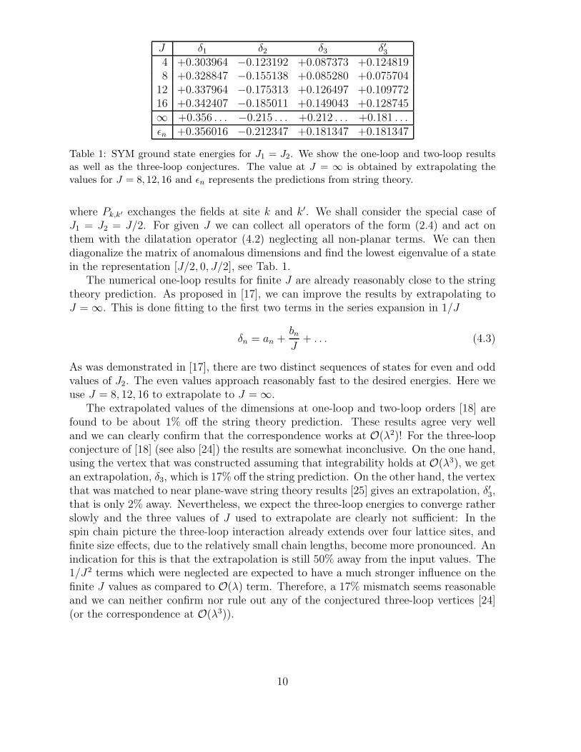
J δ1 δ2 δ3 δ′34 +0.303964 −0.123192 +0.087373 +0.1248198 +0.328847 −0.155138 +0.085280 +0.075704

12 +0.337964 −0.175313 +0.126497 +0.10977216 +0.342407 −0.185011 +0.149043 +0.128745∞ +0.356 . . . −0.215 . . . +0.212 . . . +0.181 . . .ǫn +0.356016 −0.212347 +0.181347 +0.181347

Table 1: SYM ground state energies for J1 = J2. We show the one-loop and two-loop resultsas well as the three-loop conjectures. The value at J = ∞ is obtained by extrapolating thevalues for J = 8, 12, 16 and ǫn represents the predictions from string theory.

where Pk,k′ exchanges the fields at site k and k′. We shall consider the special case ofJ1 = J2 = J/2. For given J we can collect all operators of the form (2.4) and act onthem with the dilatation operator (4.2) neglecting all non-planar terms. We can thendiagonalize the matrix of anomalous dimensions and find the lowest eigenvalue of a statein the representation [J/2, 0, J/2], see Tab. 1.

The numerical one-loop results for finite J are already reasonably close to the stringtheory prediction. As proposed in [17], we can improve the results by extrapolating toJ = ∞. This is done fitting to the first two terms in the series expansion in 1/J

δn = an +bnJ

+ . . . (4.3)

As was demonstrated in [17], there are two distinct sequences of states for even and oddvalues of J2. The even values approach reasonably fast to the desired energies. Here weuse J = 8, 12, 16 to extrapolate to J = ∞.

The extrapolated values of the dimensions at one-loop and two-loop orders [18] arefound to be about 1% off the string theory prediction. These results agree very welland we can clearly confirm that the correspondence works at O(λ2)! For the three-loopconjecture of [18] (see also [24]) the results are somewhat inconclusive. On the one hand,using the vertex that was constructed assuming that integrability holds at O(λ3), we getan extrapolation, δ3, which is 17% off the string prediction. On the other hand, the vertexthat was matched to near plane-wave string theory results [25] gives an extrapolation, δ′3,that is only 2% away. Nevertheless, we expect the three-loop energies to converge ratherslowly and the three values of J used to extrapolate are clearly not sufficient: In thespin chain picture the three-loop interaction already extends over four lattice sites, andfinite size effects, due to the relatively small chain lengths, become more pronounced. Anindication for this is that the extrapolation is still 50% away from the input values. The1/J2 terms which were neglected are expected to have a much stronger influence on thefinite J values as compared to O(λ) term. Therefore, a 17% mismatch seems reasonableand we can neither confirm nor rule out any of the conjectured three-loop vertices [24](or the correspondence at O(λ3)).

10

5 Conclusions and Outlook

In this paper we demonstrated that spectroscopy is becoming a very precise and versatiletool for establishing the validity of the AdS/CFT duality conjecture on a quantitative,dynamical level. Following the suggestion of [9, 10] and extending the earlier break-through work of [17, 11, 12] we have shown that in the non-BPS sector of two largecharges, as in the near-BPS BMN sector with single large charge [3], the duality betweenthe SYM theory and AdS5 × S5 string theory relates perturbative results on both sidesof the correspondence and thus can be tested using existing tools.

It should be fairly evident that our derivation of mathematically highly involvedenergy expressions, such as eqs.(2.7),(2.8), from both string theory and gauge theoryconstitutes a “physicist’s proof” of the correspondence. We believe that the present workis just the beginning of a much wider unraveling of dynamical details of the AdS/CFTduality. At the end, we expect to gain much insight into superstring theory on curvedbackgrounds, and into gauge theory at finite coupling.

Our work suggests a large number of further inquiries. The precise interpretation ofthe circular versus folded string solutions remains somewhat obscure in the Bethe ansatzpicture. In particular, it would be important to understand the analog of the stringsolution for J2 > J/2 in the Bethe ansatz and thus complete the picture outlined inAppendix E. Furthermore, it seems that the Bethe ansatz allows for very complicateddistributions of “Bethe root strings”, involving multi-cut solutions, the role of which isunclear so far on the string theory side.

Another obvious problem is to extend the comparison to include 1/J terms by com-puting (as in [6,10]) the 1-loop string sigma model correction to the (J1, J2) string energyand comparing the result to the leading correction to the “thermodynamic” limit of theXXX+1/2 Bethe system. It would be interesting also to compute energies of excitedstring states by expanding the superstring action near the ground-state two-spin (J1, J2)solution. In contrast to the BMN case [3], here one expects (from experience with specialcircular solutions [10]) that there will be many nearby states with the same charges andwith energies differing from the ground state energy by order 1

J 2 = λJ2 terms (these are

of course negligible as compared to similar terms in the classical ground-state energy inthe limit J ≫ 1).

It should be relatively straightforward, if laborious to extend the analysis to more thantwo spins. In string theory this has largely been accomplished for three non-vanishingangular momenta on S5 in [12], but one could try to also include concurrently the twoAdS5 charges. For gauge theory, the corresponding Bethe equations are known [16],but have not yet been analyzed in any generality. Ideally, one would like to understandhow to prove these equivalences directly, i.e. without actually solving the classical stringsigma model equations and the Bethe equations in the thermodynamic limit.

The biggest challenge clearly is to find out how to extend the calculational power oneither side of the correspondence in a way that would allow one to derive results thatare not in the overlapping window of large quantum numbers and small effective stringtension. On the string theory side, this would require to include quantum (inverse stringtension) corrections in the Green-Schwarz supercoset sigma model of [21]. For gaugetheory, we would need to understand the proper extension of the Bethe ansatz so as to

11

make it applicable to all orders in Yang-Mills perturbation theory. Maybe integrabilitywill lead the way.

Acknowledgments

We are grateful to J. Russo and K. Zarembo for useful discussions. In particular, we thankG. Arutyunov for many useful comments and help with the discussion in Appendix D.A.T. is also grateful to the organizers of Simons workshop in Mathematics and Physics atStony Brook for the hospitality at the workshop during which this paper was completed.The work of S.F. and A.T. was supported by the DOE grant DE-FG02-91ER40690. Thework of A.T. was also supported in part by the PPARC SPG 00613 and INTAS 99-1590 grants and the Royal Society Wolfson award. N.B. dankt der Studienstiftung des

deutschen Volkes fur die Unterstutzung durch ein Promotionsforderungsstipendium.

A Rotating string solutions

Let us make some general observations on 5-spin string solutions in AdS5 × S5 pointingout some relations between different types of solutions via an analytic continuation. Thegeneral rotating strings carrying 2+3 charges (S1, S2; J1, J2, J3) and the energy E aredescribed by the following ansatz [9] (see (1.3))

t = κτ , φ1 = ω1τ , φ2 = ω2τ , ϕ1 = w1τ , ϕ2 = w2τ , ϕ3 = w3τ ,

ρ(σ) = ρ(σ + 2π) , θ(σ) = θ(σ + 2π) , γ(σ) = γ(σ + 2π) , ψ(σ) = ψ(σ + 2π).(A.1)

Then the 3+3 obvious integrals of motion are11

S1 ≡S1√λ

= ω1

∫ 2π

0

dσ

2πsinh2 ρ cos2 θ , J1 ≡

J1√λ

= w1

∫ 2π

0

dσ

2πsin2 γ cos2 ψ ,

S2 ≡S2√λ

= ω2

∫ 2π

0

dσ

2πsinh2 ρ sin2 θ , J2 ≡

J2√λ

= w2

∫ 2π

0

dσ

2πsin2 γ sin2 ψ ,

E ≡ E√λ

= κ

∫ 2π

0

dσ

2πcosh2 ρ , J3 ≡

J3√λ

= w3

∫ 2π

0

dσ

2πcos2 γ .

(A.2)

They satisfy

−S1

ω1− S2

ω2+

Eκ

= 1 ,J1

w1+

J2

w2+

J3

w3= 1 . (A.3)

The second-order equations for (ρ, θ)

ρ′′ − sinh ρ cosh ρ (κ2 + τ ′2 − ω21 cos2 τ − ω2

2 sin2 τ) = 0 ,

(sinh2 ρ τ ′)′ − (ω21 − ω2

2) sinh2 ρ sin τ cos τ = 0 ,(A.4)

11As discussed in [9, 12], all other (SIJ , JMN ) generators (conserved charges) of SO(2, 4) × SO(6)except the Cartan ones E = S05, S1 = S12, S2 = S34, J1 = J12, J2 = J34, J3 = J56 should vanish inorder for the rotating string solution to represent a semiclassical string state carrying the correspondingquantum numbers.

12

and (γ, ψ)γ′′ − sin γ cos γ (w2

3 + ψ′2 − w21 cos2 ψ − w2

2 sin2 ψ) = 0 ,

(sin2 γ ψ′)′ − (w21 − w2

2) sin2 γ sinψ cosψ = 0 ,(A.5)

are decoupled from each other. As explained in [12], the resulting system of equations iscompletely integrable, being equivalent to a combination of the two Neumann dynamicalsystems. As a result, there are 2+2 “hidden” integrals of motion, reducing the generalproblem to solution of two independent systems of two coupled first-order equations,with parameters related through the conformal gauge constraint

ρ′2 − κ2 cosh2 ρ+ sinh2 ρ (θ′2 + ω21 cos2 θ + ω2

2 sin2 θ)

+ γ′2 + w23 cos2 γ + sin2 γ (ψ′2 + w2

1 cos2 ψ + w22 sin2 ψ) = 0 . (A.6)

Let us now observe the following symmetry of the above system. The two metrics in(1.3) are related by the obvious analytic continuation and change of the overall sign,which is equivalent in the present rotational ansatz (A.1) case to

ρ↔ iγ , θ ↔ ψ , κ↔ −w3 , ω1 ↔ −w1 , ω2 ↔ −w2 . (A.7)

This transformation maps the system (A.4) into the system (A.5) and also preservesthe constraint (A.6). Thus it formally maps solutions into solutions. Under (A.7) theconserved charges (A.2) (or Cartan generators of SO(2, 4)×SO(6)) transform as follows

S1 ↔ J1 , S2 ↔ J2 , E ↔ −J3 . (A.8)

We could, of course, assume instead of (A.7) that ω1, ω2 ↔ w1,w2 but then S1, S2 ↔−J1,−J2. Note that the transformed solutions may not necessarily have a natural physi-cal interpretation. In order for some two physical solutions to be related by this analyticcontinuation prescription at least one of them should have a non-vanishing J3 spin (whichtransforms into the energy of the solution).

One can find also other transformations that map solutions into solutions by combin-ing (A.7) with special (discrete) SO(2, 4) × SO(6) isometries that do not induce othercomponents of the rotation generators except the above Cartan ones (e.g., interchangingthe angular coordinates induces interchanging of the charges in (A.2), etc.). Below weshall consider such an example.

B Relation between two-spin solutions

Let us now show that the two previously known two-spin folded string solutions are, infact, related by the above analytic continuation. Firstly, there is the “(S, J)” solution [6]

κ, ω1,w3 6= 0 , ρ = ρ(σ) , θ = 0 , γ = 0 , ψ = 0 , (B.1)

where the string is stretched in the radial direction ρ of AdS5 . It rotates (ω1) in AdS5

about its center of mass which in turn moves (w3) along a large circle of S5. The gauge

13

constraint (A.7) and integrals of motion (A.2) become

w23 + ρ′2 − κ2 cosh2 ρ+ ω2

1 sinh2 ρ = 0 , J ≡ J3 = w3 ,

S ≡ S1 = ω1

∫ 2π

0

dσ

2πsinh2 ρ , E = κ

∫ 2π

0

dσ

2πcosh2 ρ .

(B.2)

Secondly, we have the “(J1, J2)” solution [11] where the string located at the center ofAdS5 is stretched (ψ) along a great circle of S5 and rotates (w2) about its center of masswhich moves (w1) along an orthogonal great circle of S5:

κ,w1,w2 6= 0 , ρ = 0 , θ = 0 , γ =π

2, ψ = ψ(σ) . (B.3)

The gauge constraint (A.7) and integrals of motion (A.2) are then

−κ2 + ψ′2 + w21 cos2 ψ + w2

2 sin2 ψ = 0 ,

E = κ , J1 = w1

∫ 2π

0

dσ

2πcos2 ψ , J2 = w2

∫ 2π

0

dσ

2πsin2 ψ .

(B.4)

Following the discussion in Appendix A we conclude that these two solutions are relatedby the following analytic continuation: 12

ρ→ iψ , κ→ −w1 , ω1 → −w2 , w3 → −κ ,E → −J1 , S → J2 , J → −E .

(B.5)

We can, in fact, directly relate the systems of equations expressing the closed stringperiodicity condition and definitions of the respective energies and spins and thus relatingthe three integrals of motion in the two cases (see, respectively, [6] and [11]). In the firstcase we get the following relations (we introduce the parameter x < 0 related to η in [6] byη = −1/x, x = − sinh2 ρ0, where ρ0 is the maximal value of the radial AdS5 coordinate)

κ2 − w23

κ2 − ω21

= − sinh2 ρ0 ≡ x < 0 , E = κ+κ

ω1S, J = w3 ,

√

κ2 − w23 =

2√−xπ

K(x) , E =2κ

√−xπ√

κ2 − w23

E(x) , (B.6)

where K(x) and E(x) are the standard elliptic integrals (see Appendix C) related to thehypergeometric functions used in [6] by

2F1(12, 1

2; 1, x) =

2

πK(x) , 2F1(−1

2, 1

2; 1; x) =

2

πE(x) . (B.7)

Solving for ω1 and κ in terms of J and x we find

ω21 = J 2 +

4

π2(1 − x)(K(x))2, κ2 = J 2 − 4

π2x (K(x))2 , (B.8)

12Note that here E − S − J → E − (J1 + J2). Choosing instead ω1 → w2, κ→ w1, w3 → κ we wouldget E → J1, S → −J2, J → E, so that E − S − J → −E + J1 + J2.

14

and then finally get the system of two equations (3.4) for the energy given in the maintext. The second of the two equations in (3.4) determines x in terms of S and J , whilethe first one then gives the energy as a function of the spins.

Similarly, for the (J1, J2) solution (B.3) one finds from the expressions given in [11](we assume w2

2 > w21)

κ2 − w21

w22 − w2

1

= sin2 ψ0 ≡ x > 0 , 1 =J1

w1+

J2

w2, E = κ,

J1 =2w1

π√

w22 − w2

1

E(x) ,√

w22 − w2

1 =2

πK(x) . (B.9)

Solving for w1, w2 in terms of J1 and x

w21 =

(

K(x)

E(x)J1

)2

, w22 =

(

K(x)

E(x)J1

)2

+4

π2K(x)2 , (B.10)

we finish with the system of the two equations determining E = E(J1,J2) given in (2.2).A manifestation of the analytic continuation relation between both two-spin solutions isthen the equivalence of the two systems (2.2) and (3.4) under the substitution (3.5) (anda continuation from x > 0 to x < 0 in the parameter space).

Depending on the region of the parameter space (or values of the integrals of motion)one finds different functional form of dependence of the energy on the two spins. Wediscuss some aspects of this dependence in Appendix E below. A direct comparison withgauge theory we are interested in here is possible in the case when the two spins S andJ are both large compared to

√λ , i.e. S ≫ 1, J ≫ 1. The analogous limit [11] for

the (J1, J2) solution is when J1 ≫ 1, J2 ≫ 1. In the two cases we can then expandthe energies, e.g., in powers of the total S5 spin J . This amounts to an expansion inpowers of J ≡ J3 in the (S, J) case and in powers of J ≡ J1 + J2 in the (J1, J2) case,respectively,

E = S + J +λ

Jǫ1(S/J) +

λ2

J3ǫ2(S/J) + . . . , J ≡ J3, S ≫

√λ ,

E = J +λ

Jǫ1(J2/J) +

λ

J3ǫ2(J2/J) + . . . , J ≡ J1 + J2, J2 ≫

√λ , (B.11)

where we introduced tildes on the correction functions ǫn in the first solution case. Onemay wonder if the coefficients ǫ1 and ǫ1 in (B.11) are related in some way, given that thetwo solutions are related by the analytic continuation. Applying formally the substitution(B.5) in (B.11) we get, to the leading order,

E = S + J +λ

Jǫ1(S/J) + . . . → −J1 = J2 − E +

λ

(−E)ǫ1(J2/(−E)) + . . . . (B.12)

Using that E = J1 + J2 + . . . in the subleading term we finish then with (where nowJ ≡ J1 + J2)

E = J − λ

Jǫ1(−J2/J) + . . . . (B.13)

15

Comparing this to (B.11) we conclude that one should have a simple relation betweenthe leading-order (“one-loop”) corrections for the energies of the two solutions:

ǫ1(j) = −ǫ1(−j) . (B.14)

As was noted in Section 3, this is indeed the relation that one finds on the gauge theoryside (3.3).

Let us now demonstrate that (B.14) follows also from the string-theory equations(B.6) and (B.9) or the systems (3.4) and (2.2). Expanding the parameter x for large Jas (with J being J1 + J2)

x = x0 +x1

J 2+x2

J 4+ . . . , (B.15)

one finds that for the (J1, J2) solution the leading value of the parameter x0 is given bythe solution of the transcendental equation

E(x0)

K(x0)= 1 − J2

J, x0 = x0(J2/J) . (B.16)

The rest of the expansion coefficients in x and the energy are then determined by linearalgebra, e.g.,

x1 = − 4(1 − x0)x0

(

K(x0) − E(x0))

E(x0)K(x0)2

π2(

(1 − x0)K(x0)2 − 2(1 − x0)K(x0)E(x0) + E(x0)2) ,

ǫ1 =2

π2K(x0) (E(x0) − (1 − x0)K(x0)) , (B.17)

ǫ2 =2

π4K(x0)

3(

(1 − 2x0)E(x0) − (1 − x0)2K(x0)

)

.

In the (S, J) case, using the same expansion (B.15) for the corresponding parameter xwhere now J = J3 we find the following equation for x0

E(x0)

K(x0)= 1 +

S

J, x0 = x0(S/J) . (B.18)

Solving this equation one finds other expansion coefficients in (B.15) and (B.11), e.g.,

x1 = − 4(1 − x0)2x0

(

K(x0) − E(x0))

E(x0)2K(x0)

π2(

(1 − x0)K(x0)2 − 2(1 − x0)K(x0)E(x0) + E(x0)2) , (B.19)

ǫ1 = − 2

π2K(x0)

(

E(x0) − (1 − x0)K(x0))

,

ǫ2 = − 2

π4K(x0)

3(

E(x0) − (1 − x20)K(x0)

)

.

Comparing (B.16),(B.19) to (B.18),(B.17) and observing that to leading order (B.5)implies J2 → S, J → −J , we indeed confirm the relation (B.14).

16

C Gauge theory details

Here we will outline the solution of the Bethe ansatz system of equations (3.2) for thenovel case of the XXX−1/2 Heisenberg spin chain. We expect that the positions of theroots are of order O(J), where J is the length of our non-compact magnetic chain, asexplained in Section 3. We then take the logarithm of the equations (3.2) and obtain forlarge J

− J

uj

= 2πnj + 2S

∑

k=1k 6=j

1

uj − uk

, δ1 =J

8π2

S∑

j=1

1

u2j

. (C.1)

The mode numbers nj enumerate the possible branches of the logarithm. Excitingly,we see that these large J equations are almost identical to the ones found in [17] forthe compact XXX+1/2 chain (cf. eq.(2.7) in [17]), except for a minus sign on the lefthand side of the left equation in (C.1). It therefore does not come as a surprise thatthe solution will be very similar to the previously considered case. The differences are,however, very interesting, and we will briefly rederive the solution for the new case (C.1).

As in the case of the XXX+1/2 system, we shall start with assuming that in the largeJ limit the Bethe roots accumulate on smooth contours. It is reasonable, therefore, toreplace the discrete root positions uj by a (rescaled) smooth continuum variable u andintroduce a density ρ(u) describing the distribution of the roots in the complex u-plane:

uj

J→ u with ρ(u) =

1

J

S∑

j=1

δ(

u− uj

J

)

. (C.2)

For the operators in eq.(3.1) with one AdS5 charge S there are precisely S roots, andthe density is normalized to the filling fraction β = S/J ,

∫

C

du ρ(u) = β, (C.3)

where C is the support of the density, i.e. the union of contours along which the roots aredistributed. The Bethe equations (C.1) in the “thermodynamic limit” then convenientlyturn into singular integral equations:

−∫

C

dv ρ(v) u

v − u=

1

2+ π nC(u) u, δ1 =

1

8π2

∫

C

du ρ(u)

u2(C.4)

where nC(u) is the mode number at point u. It is expected to be constant along eachcontour. Here and in the following the slash through the integral sign implies a principalpart prescription. In addition, we have the momentum conservation condition, resultingfrom the cyclic boundary conditions of our chain:

S∏

j=1

uj + i/2

uj − i/2= 1 , i.e.

∫

C

du ρ(u)

u= 0 and

∫

C

du ρ(u)nC(u) = 0, (C.5)

where the last equation is a consistency condition derived from the left eq.(C.1) bysumming both sides of that equation over all j.

17

As opposed to the XXX+1/2 case, we expect the roots for the ground state to lie onthe real axis (this may be verified by explicit solution of the exact Bethe equations forsmall values of J). Furthermore, we assume the distribution of roots to be symmetricw.r.t. the imaginary axis, ρ(−u) = ρ(u). We therefore expect the support of the rootdensity to split into (at least) two disjoint intervals C = C− + C+ with C− = [−b,−a]and C+ = [a, b], where a < b are both real.13 For the ground state we expect just twocontours, and the mode numbers should be n = ∓1 on C±. For this distribution of roots,the Bethe equations (C.4) become

−∫ b

a

dv ρ(v) u2

v2 − u2=

1

4− π

2u , δ1 =

1

4π2

∫ b

a

du ρ(u)

u2. (C.6)

Comparing to the previous solution in [17], we thus find an identical equation exceptthat the new filling fraction β = S

Jis related to the previous one α = J2

Jby β → −α! 14

Interestingly, we already analyzed the case of negative α, i.e. positive β as a technicaltrick in [17]; here we find that this case, which did not previously correspond to a physicalsituation for the spin +1

2chain, is physical in the case of the −1

2chain. The solution of the

integral equation (see, e.g., [26]), yielding the density ρ(u), may be obtained explicitly(in [17] we rather eliminated the density after obtaining an integral representation forit); it reads

ρ(u) =2

πu−∫ b

a

dv v2

v2 − u2

√

(b2 − u2)(u2 − a2)

(b2 − v2)(v2 − a2). (C.7)

This density may be expressed explicitly through standard functions:

ρ(u) =1

2πbu

√

u2 − a2

b2 − u2

[

b2

a− 4u2Π

(

b2 − u2

b2, q

)]

, q =b2 − a2

b2, (C.8)

where we introduced the modulus q, playing the role of an auxiliary parameter, and Πis the elliptic integral of the third kind:

Π(m2, q) ≡∫ π/2

0

dϕ

(1 −m2 sin2 ϕ)√

1 − q sin2 ϕ. (C.9)

Furthermore, we may derive two conditions determining the interval boundaries a, b asa function of the filling fraction β:

∫ b

a

du u2

√

(b2 − u2)(u2 − a2)=

1 + 2β

4and

∫ b

a

du√

(b2 − u2)(u2 − a2)=

1

4ab.

(C.10)The first is derived from the normalization condition eq.(C.3), while the second is aconsistency condition, assuring the positivity of the density. These may be reexpressed

13After the analytical continuation to the spin + 1

2case, the points a, b become a complex conjugate

pair.14To facilitate comparison, note that here we are using a different convention for normalizing the

density.

18

through standard elliptic integrals of, respectively, the second and the first kind; onefinds

E(q) ≡∫ π/2

0

dϕ

√

1 − q sin2 ϕ =1 + 2β

4b, K(q) ≡

∫ π/2

0

dϕ√

1 − q sin2 ϕ=

1

4a(C.11)

It is straightforward to eliminate the interval boundaries a, b from these equations; fur-thermore, we can integrate the density and compute the energy δ1 from the right equationin eqs.(C.6) (cf. (2.8))

δ1 =1

2π2K(q)

(

(2 − q)K(q) − 2E(q))

, β ≡ S

J=

1

2√

1 − q

E(q)

K(q)− 1

2. (C.12)

Finally, we can also express the boundaries of the Bethe strings through the modulus q:

a =1

4K(q), b =

1

4√

1 − qK(q). (C.13)

This completes the solution.

D The circular vs. imaginary solution

In [17] a solution different from the type discussed in Appendix C was found. Theresulting anomalous dimension matched the energy of a circular string [9] at one point ofthe parameter space, J2 = J1 = J/2. Recently the circular string solution was extendedto all values of J2 [12] where it was also shown that the agreement with gauge theorypersists up to a few orders in a perturbative expansion around J2 − J/2. Here, we willcomplete the analysis and prove the correspondence at the analytic level. We are gratefulto Gleb Arutyunov for his collaboration on this Appendix. Without further details ofthe derivation, we present the final results starting with gauge theory.

There are two conditions on the endpoints is, it, s < t, of the Bethe strings that arisein the solution [17] (α = J2/J):

∫ s

−s

dv v2

√

(s2 − v2)(t2 − v2)=

1 − 2α

4and

∫ s

−s

dv√

(s2 − v2)(t2 − v2)=

1

4st. (D.1)

Notice the great similarity to (C.10)! We perform the elliptic integrals and get

K(r) − E(r) =1 − 2α

8t, K(r) =

1

8s, r =

s2

t2. (D.2)

The differences to (C.11) are due to the different regions of integration. Solving fors, t and substituting in the expression for the energy (we use the notation δ and ǫ todistinguish the circular solution)

δ1 =1

32π2

(

1

s2+

1

t2− 2(1 − 2α)

st

)

(D.3)

19

we get the one-loop result from gauge theory

δ1 =2

π2K(r)

(

2E(r) − (1 − r)K(r))

, α ≡ J2

J=

√r − 1

2√r

+1

2√r

E(r)

K(r). (D.4)

The circular string is obtained by the same ansatz (B.3) as for the folded string (seeAppendices A,B). The only difference is that the function ψ(σ) is now assumed to beperiodic modulo 2π

ψ(σ + 2π) = ψ(σ) + 2π. (D.5)

Instead of folding back into itself, the string wraps completely around a great circle. Theset of equations that describes this circular string are [12]

J2 =w2

y

(

1 − E(y)

K(y)

)

, J1 =w1

y

(

y − 1 +E(y)

K(y)

)

,

E2 = w21 +

w22 − w2

1

y, K(y) =

π

2

√

w22 − w2

1

y.

(D.6)

When solved for w1,w2 we get a system of two equations similar to the one in (2.2)( E

K(y)

)2

−(

yJ1

(1 − y)K(y)− E(y)

)2

=4

π2,

(

yJ2

K(y) − E(y)

)2

−(

yJ1

(1 − y)K(y)− E(y)

)2

=4

π2y. (D.7)

The ansatz for the circular solution is symmetric under J1 ↔ J2, but superficially thisdoes not seem to apply to these equations. Indeed, a modular transformation is requiredto interchange J1,J2:

K(y) =√

1 − y′ K(y′), E(y) =E(y′)√1 − y′

, y = 1 − 1

1 − y′. (D.8)

In order to make contact with gauge theory, we set y = y0 + y1/J 2 + . . . and expand theenergy in powers of 1/J 2. Using the expansion (2.3) we find

ǫ1 =2

π2K(y0)E(y0), α ≡ J2

J=

1

y0

− E(y0)

y0 K(y0). (D.9)

As before, the string solution (D.9) is related to the gauge solution (D.4) through amodular transformation

K(y0) = (1 −√r)K(r), E(y0) = 2(1 −√

r)−1E(r) − (1 +√r)K(r) (D.10)

where

y0 = − 4√r

(1 −√r)2

= − 4ab

(b− a)2. (D.11)

Note that the integration constant of the circular string y is related to the integrationconstant of the folded string x by y = 1/x. The gauge theory constants a = is, b = itdescribe the endpoints of some Bethe strings. Remarkably, (D.11) is exactly the samerelation as in the case of the folded string (2.9)!

20

-2.5 -2 -1.5 -1 -0.5 0 0.5 1J2�J=-S�J

-0.5

0

0.5

1

1.5

2

Ε1HJ2�JL=-Ε~

1HS�JL

half-

filli

ng

BMN limit

HJ1,J2L

Ε1

Ε`

1

HS,JL

- Ε

~

1¬ ~log2

HS�JL

~

1�����������������������������������

1-

J 2�J®

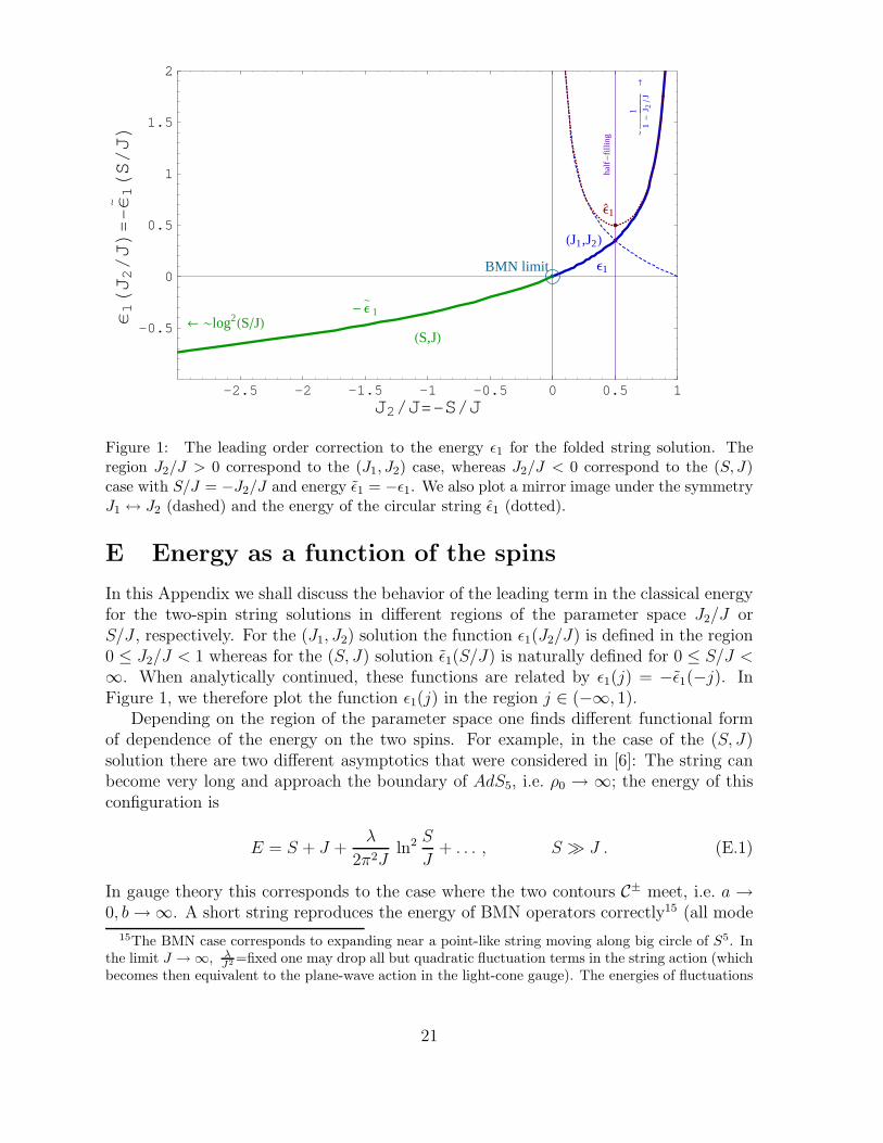
Figure 1: The leading order correction to the energy ǫ1 for the folded string solution. Theregion J2/J > 0 correspond to the (J1, J2) case, whereas J2/J < 0 correspond to the (S, J)case with S/J = −J2/J and energy ǫ1 = −ǫ1. We also plot a mirror image under the symmetryJ1 ↔ J2 (dashed) and the energy of the circular string ǫ1 (dotted).

E Energy as a function of the spins

In this Appendix we shall discuss the behavior of the leading term in the classical energyfor the two-spin string solutions in different regions of the parameter space J2/J orS/J , respectively. For the (J1, J2) solution the function ǫ1(J2/J) is defined in the region0 ≤ J2/J < 1 whereas for the (S, J) solution ǫ1(S/J) is naturally defined for 0 ≤ S/J <∞. When analytically continued, these functions are related by ǫ1(j) = −ǫ1(−j). InFigure 1, we therefore plot the function ǫ1(j) in the region j ∈ (−∞, 1).

Depending on the region of the parameter space one finds different functional formof dependence of the energy on the two spins. For example, in the case of the (S, J)solution there are two different asymptotics that were considered in [6]: The string canbecome very long and approach the boundary of AdS5, i.e. ρ0 → ∞; the energy of thisconfiguration is

E = S + J +λ

2π2Jln2 S

J+ . . . , S ≫ J . (E.1)

In gauge theory this corresponds to the case where the two contours C± meet, i.e. a →0, b→ ∞. A short string reproduces the energy of BMN operators correctly15 (all mode

15The BMN case corresponds to expanding near a point-like string moving along big circle of S5. Inthe limit J → ∞, λ

J2 =fixed one may drop all but quadratic fluctuation terms in the string action (whichbecomes then equivalent to the plane-wave action in the light-cone gauge). The energies of fluctuations

21

numbers are n = ±1)

E = J + S +λS

2J2+ . . . , S ≪ J . (E.2)

One may also consider a “near BMN” limit S/J ≪ 1 of the two-spin solution keepingfull dependence on λ. Then we get

E = J + S

√

1 +λ

J2− λS2

4J3· 2 + λ/J2

1 + λ/J2+ . . . , S ≪ J , (E.3)

This gives the near BMN limit for a total of S excitations of modes n = ±1. Note,however, that we must consider a large number of excitations S = O(J), i.e. S = βJwith β small but O(J0). Therefore, we may not assume that S = βJ takes a particular,finite value like, for example, two (in an attempt to compare to 1/J terms in [25]).Instead, one must consider an arbitrary number of excitations S and consider only thecoefficient c in the near BMN correction (cS + c′)/J = cβ + O(1/J). The point is thatc′ is an O(1/J) correction which we presently ignore.

At S/J = 0 we make the “Wick-rotation” to the (J1, J2) solution. The energy of ashort string rotating on S5 is given by

E = J +λ J2

2J2+ . . . , J2 ≪ J , (E.4)

where we can explicitly see the connection to the (S, J) case. Similarly, the near BMNlimit reads (we set J1 = J to compare to BMN terminology, J2 represents the numberof excitations)

E = J1 + J2

√

1 +λ

J21

− λ J22

4J31

· 2 + 3λ/J21

1 + λ/J21

+ . . . , J2 ≪ J . (E.5)

As the charge J2 increases, the string grows until for J1 = J2 we get

E = J + cλ

J+ . . . , c ≡ ǫ1(1/2) = 0.356016 . . . , J2 = J1 = J/2 . (E.6)

In string theory nothing special happens, the string extends over approximately 120◦ andcan grow further. In contrast, in gauge theory we made the assumption J2 ≤ J1 to solvethe Bethe ansatz. Therefore, we do not get solutions beyond this point. Nevertheless, interms of charges, we can freely interchange J1 and J2. The string solutions for J2 > J/2should correspond to some gauge theory states with J2 < J/2

δ′1(J2/J) = ǫ1(1 − J2/J) , for 0 ≤ J2 ≤ J/2 . (E.7)

We see that the string energy ǫ1(J1, J2) is not symmetric with respect to J1 ↔ J2. Asa consequence, the anomalous dimensions δ′1(J1, J2) do not belong to operators with the

above the BPS ground state E = J are then determined by the string fluctuation masses given bym2 = 1

J 2 = λJ2 .

22

minimal energy, δ1(J1, J2), but to some other set of operators with larger dimensions.That suggests that one and the same string solution describes two different operatorsin different regions of parameter space. There are some indications16 that these newgauge theory operators are the odd, unpaired ground state solutions found in [17]. Thisis an interesting possibility, as it would explain why for half-filling, J2 = J/2, the odd,unpaired ground state has energy (E.6) as suggested by numerical evidence [17]. Furthernumerical evidence shows that the anomalous dimension δ′1 of this state near J2 = 0scales as 1/J2 instead of 1/J . Indeed, this is what happens on the string theory side.The largest extension of the S5 solution takes place near J2 = J . Then the string extendsover half a great circle and the energy is 17

E = J +2 λ

π2 J(1 − J2/J)+ . . . = J +

2 λ

π2 J1+ . . . , J2 ≈ J . (E.8)

At J2 = J the folded string becomes, in fact, equivalent to a different configuration: Onehalf of the string can be unfolded to give the circular string discussed in Appendix D.It is interesting to see that also the energy of the circular solution ǫ1 asymptotes to thesame value

E = J +2 λ

π2 J1+ . . . , J2 ≈ J . (E.9)

The energy ǫ1 of the circular solution decreases as we decrease J2 up to half-fillingJ2 = J1 = J . Unlike in the case of the folded string, the energy has a minimum

E = J +λ

2J+ . . . , J2 = J1 = J/2 . (E.10)

Furthermore, the solution ǫ1 is symmetric under J1 ↔ J2 and we can stop.

References

[1] J. M. Maldacena, “The large N limit of superconformal field theories and supergravity”,Adv. Theor. Math. Phys. 2 (1998) 231, hep-th/9711200. • S. S. Gubser, I. R. Klebanovand A. M. Polyakov, “Gauge theory correlators from non-critical string theory”,Phys. Lett. B428 (1998) 105, hep-th/9802109. • E. Witten, “Anti-de Sitter space andholography”, Adv. Theor. Math. Phys. 2 (1998) 253, hep-th/9802150.

[2] G. Arutyunov, S. Frolov and A. C. Petkou, “Operator product expansion of the lowestweight CPOs in N = 4 SYM4 at strong coupling”, Nucl. Phys. B586 (2000) 547,hep-th/0005182. • B. Eden, A. C. Petkou, C. Schubert and E. Sokatchev, “Partialnon-renormalisation of the stress-tensor four-point function in N = 4 SYM4 andAdS/CFT”, Nucl. Phys. B607 (2001) 191, hep-th/0009106. • G. Arutyunov,F. A. Dolan, H. Osborn and E. Sokatchev, “Correlation functions and massiveKaluza-Klein modes in the AdS/CFT correspondence”, Nucl. Phys. B665 (2003) 273,hep-th/0212116.

16Apparently, solutions to the Bethe equations with J2 > J/2 correspond to mirror images of solutionswith J ′

2= J + 1 − J2 ≤ J/2 (s 7→ −1 − s with SU(2) spin s = J/2 − J2). If we assume J2 and J to be

even, in this way we would find solutions with odd J ′2 and even J , i.e. the odd, unpaired ground states.

17Since the one-loop correction ǫ1 grows to infinity at J2 ≈ J the string solution is not stable at largeenough J2.

23

[3] D. Berenstein, J. M. Maldacena and H. Nastase, “Strings in flat space and pp wavesfrom N = 4 Super Yang Mills”, JHEP 0204 (2002) 013, hep-th/0202021.

[4] M. Blau, J. Figueroa-O’Farrill, C. Hull and G. Papadopoulos, “A new maximallysupersymmetric background of IIB superstring theory”, JHEP 0201 (2002) 047,hep-th/0110242. • R. R. Metsaev, “Type IIB Green-Schwarz superstring in plane waveRamond-Ramond background”, Nucl. Phys. B625 (2002) 70, hep-th/0112044.

[5] S. S. Gubser, I. R. Klebanov and A. M. Polyakov, “A semi-classical limit of thegauge/string correspondence”, Nucl. Phys. B636 (2002) 99, hep-th/0204051.

[6] S. Frolov and A. A. Tseytlin, “Semiclassical quantization of rotating superstring inAdS5 × S5”, JHEP 0206 (2002) 007, hep-th/0204226.

[7] A. A. Tseytlin, “Semiclassical quantization of superstrings: AdS5 × S5 and beyond”,Int. J. Mod. Phys. A18 (2003) 981, hep-th/0209116.

[8] J. G. Russo, “Anomalous dimensions in gauge theories from rotating strings inAdS5 × S5”, JHEP 0206 (2002) 038, hep-th/0205244. • J. A. Minahan, “Circularsemiclassical string solutions on AdS5 × S5”, Nucl. Phys. B648 (2003) 203,hep-th/0209047. • G. Mandal, N. V. Suryanarayana and S. R. Wadia, “Aspects ofsemiclassical strings in AdS5”, Phys. Lett. B543 (2002) 81, hep-th/0206103.

[9] S. Frolov and A. A. Tseytlin, “Multi-spin string solutions in AdS5 × S5”,Nucl. Phys. B668 (2003) 77, hep-th/0304255.

[10] S. Frolov and A. A. Tseytlin, “Quantizing three-spin string solution in AdS5 × S5”,JHEP 0307 (2003) 016, hep-th/0306130.

[11] S. Frolov and A. A. Tseytlin, “Rotating string solutions: AdS/CFT duality innon-supersymmetric sectors”, Phys. Lett. B570 (2003) 96, hep-th/0306143.

[12] G. Arutyunov, S. Frolov, J. Russo and A. A. Tseytlin, “Spinning strings in AdS5 × S5

and integrable systems”, hep-th/0307191.

[13] H. J. de Vega and I. L. Egusquiza, “Planetoid String Solutions in 3 + 1 AxisymmetricSpacetimes”, Phys. Rev. D54 (1996) 7513, hep-th/9607056.

[14] A. Santambrogio and D. Zanon, “Exact anomalous dimensions of N = 4 Yang-Millsoperators with large R charge”, Phys. Lett. B545 (2002) 425, hep-th/0206079.

[15] J. A. Minahan and K. Zarembo, “The Bethe-ansatz for N = 4 super Yang-Mills”,JHEP 0303 (2003) 013, hep-th/0212208.

[16] N. Beisert and M. Staudacher, “The N = 4 SYM Integrable Super Spin Chain”,Nucl. Phys. B670 (2003) 439, hep-th/0307042.

[17] N. Beisert, J. A. Minahan, M. Staudacher and K. Zarembo, “Stringing Spins andSpinning Strings”, JHEP 0309 (2003) 010, hep-th/0306139.

[18] N. Beisert, C. Kristjansen and M. Staudacher, “The dilatation operator of N = 4conformal super Yang-Mills theory”, Nucl. Phys. B664 (2003) 131, hep-th/0303060.

[19] N. Beisert, “The Complete One-Loop Dilatation Operator of N = 4 Super Yang-MillsTheory”, hep-th/0307015.

[20] I. Bena, J. Polchinski and R. Roiban, “Hidden symmetries of the AdS5 × S5

superstring”, hep-th/0305116.

24

[21] R. R. Metsaev and A. A. Tseytlin, “Type IIB superstring action in AdS5 × S5

background”, Nucl. Phys. B533 (1998) 109, hep-th/9805028.

[22] L. Dolan, C. R. Nappi and E. Witten, “A Relation Between Approaches to Integrabilityin Superconformal Yang-Mills Theory”, hep-th/0308089.

[23] A. V. Belitsky, A. S. Gorsky and G. P. Korchemsky, “Gauge/string duality for QCDconformal operators”, Nucl. Phys. B667 (2003) 3, hep-th/0304028.

[24] N. Beisert, “Higher loops, integrability and the near BMN limit”, hep-th/0308074.

[25] C. G. Callan, Jr., H. K. Lee, T. McLoughlin, J. H. Schwarz, I. Swanson and X. Wu,“Quantizing string theory in AdS5 × S5: Beyond the pp-wave”, hep-th/0307032.

[26] I. K. Kostov and M. Staudacher, “Multicritical phases of the O(n) model on a randomlattice”, Nucl. Phys. B384 (1992) 459, hep-th/9203030. • N. Muskhelishvili, “Singularintegral equations”, Noordhoff NV (1953), Groningen, Netherlands.

25